Submitted:
08 October 2024
Posted:
09 October 2024
You are already at the latest version
Abstract
Controlling an object that is extremely prone to oscillations is a complex and highly relevant task. The tendency to oscillate arises due to the presence of an oscillatory element and a delay element, and control is often complicated by the presence of an integrator in the object. For such objects, a very effective method of numerical optimization of the controller is not effective enough without choosing the most efficient structure, more efficient than the PID controller and even than the PIDD controller. The method of using the Smith predictor, which is switched on parallel to the plant, allows solving a similar problem, but the resulting quality of control remains not good enough, since a large overshoot remains in the system. The article recommends, after using the Smith predictor, to additionally use an external control loop, the sequential controller of which should also be designed using the numerical optimization method. But the Smith predictor is not the best solution either. The article recommends the use of pseudo-local feedback. Such a connection provides more opportunities, since its structure and parameters can be optimized, while the Smith predictor in its parameters is completely determined by the object model and its modification is not allowed. The article shows that even the best sequential controller in the case of using the Smith predictor on a test example still cannot provide the required quality of control; in such a system, significant overshoot remains, more than 10%. The proposed method allows reducing overshoot to less than 0.5%. It is shown that the resulting system is robust, since the quality of control remains within specified limits even when the gain changes by 30% in both directions.
Keywords:
Controllers
; PID
; Optimization
; Modeling
; Simulation
; Smith predictor
; multi-loop system
; pseudo-local feedback
MSC: 93B51
2 Institute of Laser Physics, Siberian Branch of the Russian Academy of Sciences, Lavrentiev Avenue, 15b. Russia, Novosibirsk
1. Introduction
One of the most difficult objects to control is an object that is extremely prone to oscillations, especially if in its mathematical model, in addition to the oscillatory link, there is also an integrating link and a pure delay link [1,15,16,17,18,19,20,21,22]. In particular, actuators for automatically focusing optical systems with magnetic control, based on the design of fastening the focusing lenses, can be divided into string-mounted and rod-mounted. The string suspension has a number of undeniable advantages, including high speed and the complete absence of dry friction, which allows for wide-band control with zero static error. These designs are much simpler and cheaper, and therefore more reliable, but they are not widely used in optical disk drives precisely because of the difficulty of controlling vibrations. For such objects, the use of a traditional sequential regulator is not effective enough. It is necessary to use multi-loop structures.
The structure with the Smith predictor is widely known [15,16,17,18,19,20,21,22], however, it also has some disadvantages, so that it does not always provide sufficiently high-quality control. Quality indicators are overshoot, which should be as small as possible, oscillations, which should not exist if possible, or they should decay very quickly, as well as the duration of the transition process. Quality indicators describe dynamic error.
This article examines an alternative way to control such an object and demonstrates that more effective technical solutions can be obtained, in particular, pseudo-local feedback in combination with an additional external loop that provides astatic control.
2. Materials and Methods
2.1. Theory
The calculation of the regulator is carried out on the basis of a mathematical model of the object and using the theory of how exactly this calculation should be carried out. Historically, there has been a preference for methods that make it possible to first find a solution to a problem in a general form, after which the parameters of the object model are substituted into this general solution to obtain the desired parameters of the controller. But this path is not applicable to the problem of controller synthesis, since it is too complex and does not have solutions in a general analytical form. Therefore, the numerical optimization method is more effective.
2.1. Aproach
The numerical optimization method consists of choosing a controller structure for a given object model, choosing an objective function for optimization, choosing a software tool for mathematical modeling and its operating modes, and launching an optimization program for specific numerical values of all parameters of the object model.
If the object is linear, then its mathematical model, as a rule, is specified in the form of a transfer function in the domain of the Laplace transform. It is equal to the ratio of the output signal to the input signal in Laplace image space. In the space of signals as functions of time, this dependence is much more complex, since it would be necessary to use the operations of integration and differentiation in cases where in the domain of Laplace transforms these are just operations of division or multiplication by argument s, which is close in meaning to the concept of frequency, but not identical to it concept.
In the general case, a structure with negative feedback is a serial connection of a controller and an object, after which the output of the object with a negative sign is connected through an adder to the input of the controller, and the second input of this adder receives the prescribed value for the output quantity, which is called a reference and is denoted by v(t). Structures that are more complex can also be used. The most commonly used controller is the PID controller [1,2,3,4,5,6,7,8,9,10,11,12,13,14], which contains proportional, integrating and differentiating channels.
The transfer function of the PID controller has the following form:
Here Kp, Ki, Kd are the controller coefficients, s is the argument of the Laplace transform. If the object model has an integrator, then the integral channel in the controller is not required, and a PD controller is sufficient, that is, controller (1), in which KI = 0. If the order of the object is too large, it may also be possible to use a channel that has double differentiation; in this case, the controller model is called PIDD, or PID2 controller [23,24]. Its transfer function has the following form:
Structures that are more complex may contain circuits that are included, for example, in parallel to the object model, as is the case with the Smith predictor. If the object has a transfer function in the form of the product of the minimum-phase transfer function, described by a fraction in the form of a ratio of two polynomials of the argument s and a pure delay link, described by an exponent of s with a negative real coefficient, then the Smith predictor can be used, and it is included in parallel to the model object, and feedback is taken not from the output of the object, but from the output of the adder, which sums the output signal of the object with the output signal of the Smith predictor.
A controller with local feedback can be used if at least one signal at some intermediate point of the object model is available for measurement. If such a signal is not available, then it can be artificially obtained using a model of the object or part of it. In this case, the local feedback signal is taken not from the object, but from its model, and not local feedback, but pseudo-local feedback is created.
2.3. Formulation of the Problem
Let’s consider an object that is highly prone to oscillation, since it contains an oscillatory link with a high quality factor, as well as an integrator and a delay link, which prevent the suppression of this oscillation due to deep negative coupling. The transfer function WO(s) of the object is given by the following relation in the operator domain.
The first two factors represent the minimum-phase part of the transfer function, and the third factor is the pure delay link.
It is required to design and calculate a controller that will ensure that the response of a system covered by negative feedback to the input reference signal is as close as possible to the response of a linear link with a transfer function equal to unity. In other words, the output value of the system must repeat the input signal as accurately as possible, with minimal dynamic distortion and zero static error.
2.4. Method
Traditionally, for such tasks, the system structure used is proposed in the form of a system with a single negative feedback and a sequential regulator at the input. If such a solution turns out to be insufficient, then the structure of the regulator becomes more complicated.
Traditionally, objects are considered, first of all, the possibility and feasibility of using a PID controller (1), but since the object itself contains an integrator, the structure of the PID controller should be divided into the transfer function of the integrator, and in this case we obtain the structure of the PID controller (2) [23,24].
To calculate the coefficients of this controller, it is proposed to use modeling and numerical optimization in the VisSim software, which is specially designed for such tasks. The rationale for this choice is given in many of our articles [25,26,27]. The block diagram of the object in this software has the form shown in Figure 1. The block diagram of the system is shown in Figure 2. Blogs in the form of pentagons with the letters p, d, dd are amplifiers with gain factors indicated by these labels, and the value of these coefficients, those. the values of the coefficients in the controller equation (2) are calculated in the numerical optimization procedure. Here the letter designation corresponds to the coefficient index in the regulator (2).
To carry out optimization, special blocks called “parameter Unknown” and “Cost” are used. Each block “parameter Unknown” is the input and output for the built-in optimization program; the starting values of this parameter are supplied to its input, and the current values are taken from its output at each test stage. In order for the blog to work, any constant with which the search begins, for example, a zero or one value, must be supplied as its input. The output of this blog should be connected to a bus marked with the same label that marks the corresponding coefficients, the value of which you want to find. In this case, there will be three blocks with outputs connected to labels p, d, dd. In order for the optimization result to be known, the outputs of these labels are connected to indicators showing the final value of the calculated parameters. In addition, optimization requires calculating the value of the cost function, which is the criterion for achieving the optimum; this input is the input of the “Cost” block.
The method also involves the formation of a test signal, which, as a rule, for linear systems is a single jump, that is, a function of the following form:
Here t – time from the beginning of each modeling step. Signals that are a function of time circulate in the system; they are designated in lowercase Latin letters. The Laplace representation of each such signal is indicated using capital letters, and the argument in this case is the complex frequency, denoted by the symbol s.
First, let’s set the simulation time T = 80 s. Let the maximum number of iterations will be set 5000. Using the integration method, we’ll choose the simple Euler method, sampling step 0.1 s.
The cost function F(T) in the following form:
Here e(t) is the control error calculated at the output of the subtracting device, indicated by this letter on the bus in Figure 2, k is the weighting coefficient in this cost function, which by default is chosen to be large enough, for example, k = 100. The justification for such a cost function is given in our publications [24,25,26,27].
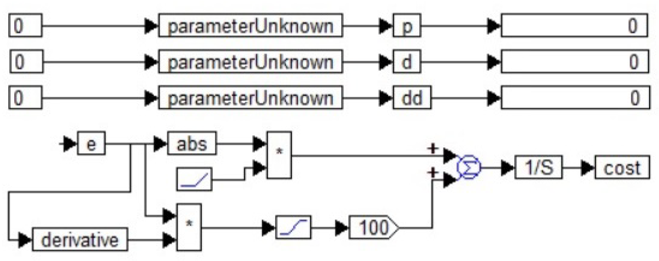
Figure 3.
Structure for modeling an optimization block based on a cost function (5).
Numerical optimization of the traffic control regulator for this object does not lead to success. The result is an unstable system. Instability manifests itself in the form of oscillations at a frequency near the resonance frequency of a second-order high-Q filter within the object. The amplitude of these oscillations is up to 30% of the amplitude of the input step and gradually increases. Even adding a triple differentiation channel does not solve the problem.
Thus, a more efficient solution is required to manage such a facility.
The Smith predictor can also be used [15,16,17,18,19,20,21,22]. The structure of the Smith predictor consists of a complete model of the object, to which a differential amplifier is added, which is the output of this predictor. The positive input of the differential amplifier is connected to the output of the minimum-phase part of the object model, and the negative input is connected to the output of the full object model. The Smith predictor is switched on in parallel to the controlled object. For the considered object (3), the transfer function of the Smith predictor has the following form:
If the resulting system is not efficient enough, you can try adding another circuit external to this system. This can further improve the quality of the transient process, including ensuring zero static error and improving the quality of the process, that is, reducing or completely eliminating overshoot, reducing the duration of the transient process, and suppressing residual oscillations if they are present.
The peculiarity of the transfer function of the Smith predictor (6) is that, firstly, in the high-frequency region it is quite close to the object transfer function (3), and secondly, in the zero-frequency region it is close to zero.
Developing this idea, we can propose to abandon the Smith predictor, replacing it with a simplified model that also has these two features. In particular, one can offer pseudo-local feedback.
3. Results
3.1. Results of the Firest Approach
Figure 4 shows the result of optimization of a system with a PID3 controller and a Smith predictor. The corresponding transient process in such a system is shown in Figure 5.
Values of the obtained coefficients: kP = 1.198 ≈ 1.2, kd = 4.669 ≈ 4.67, kdd = 13.685 ≈ 13.7, kd 3 = 1.256 ≈ 1.26. Thus, the controller equation has the form:
The overshoot in this system is 9%, as can be seen from the graph in Figure 5. The process duration is about 22 s.
The obtained result can be improved due to the external loop, which covers the resulting system as a new control object. In this case, we will leave the calculated coefficients of the PD3 controller of the internal loop fixed in accordance with relation (7) and keep the Smith predictor according to relation (6), connected in parallel to the plant, and cover this entire system with a loop with a unit negative feedback and with a PID controller in direct control channel.
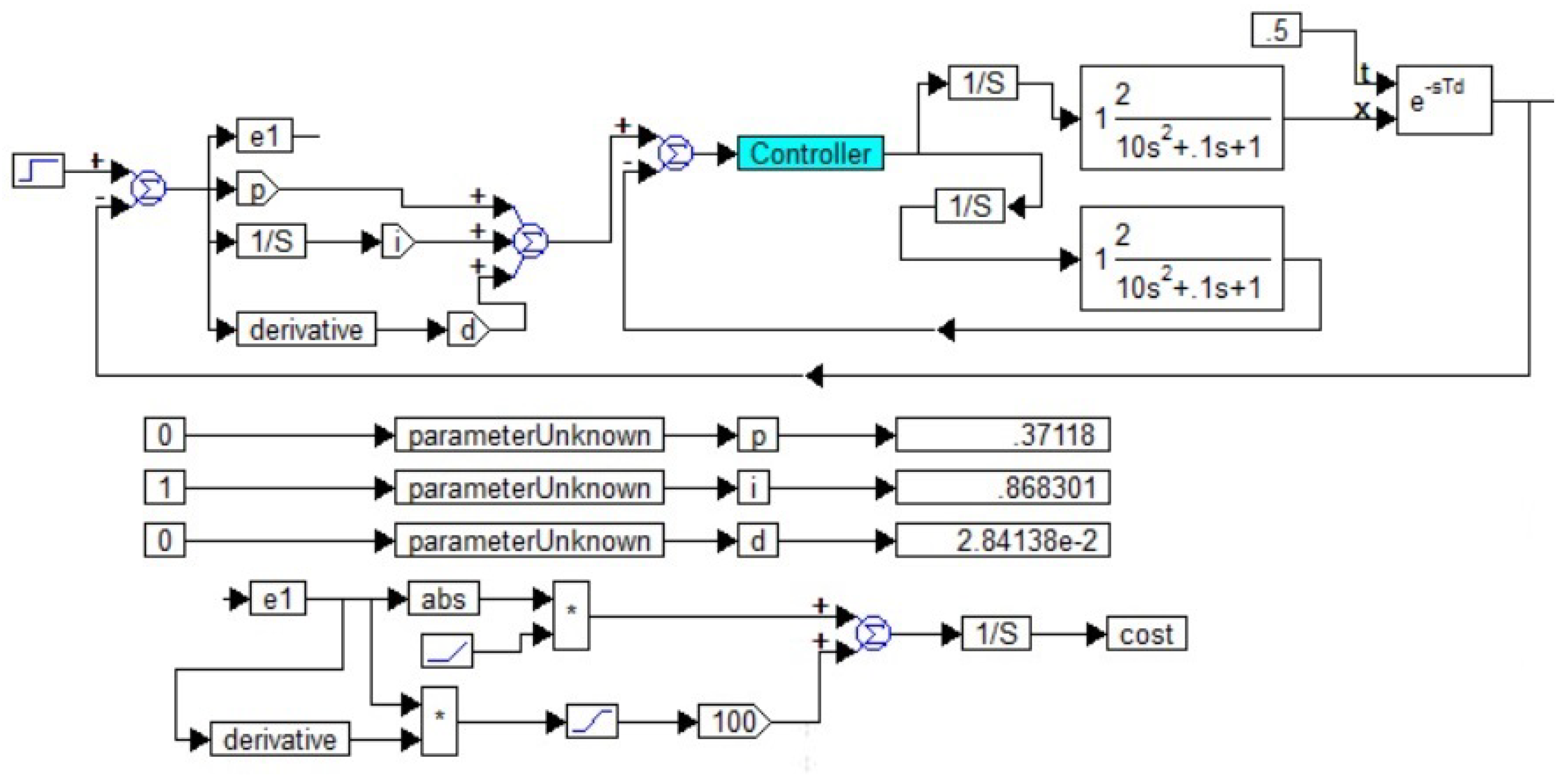
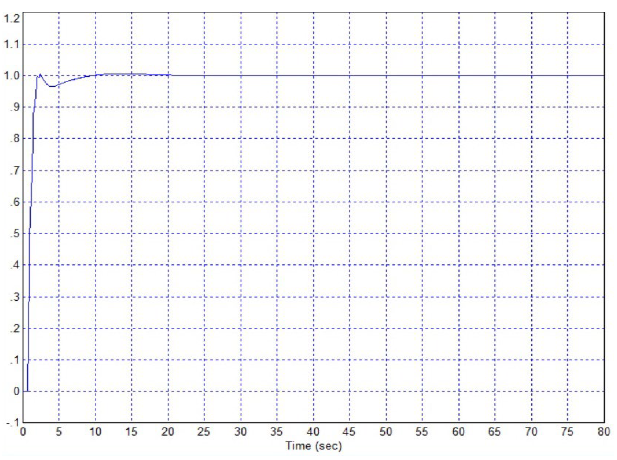
Figure 6.
Structure for modeling and optimization of a system with an external loop around a system with a PD3 controller and a Smith predictor according to Figure 4.
Figure 6.
Structure for modeling and optimization of a system with an external loop around a system with a PD3 controller and a Smith predictor according to Figure 4.
Figure 7.
Transient process in the system according to Figure 6.
Figure 7.
Transient process in the system according to Figure 6.
Values of the obtained external loop coefficients: k P = 0.37118 ≈ 0.37, k i = 0.8683 ≈ 0.868, k d = 0.0284 ≈ 0.03. Thus, the controller equation has the form:
Overshoot in this system is less than 0.5%, as can be seen from the graph in Figure 5, that is, there is practically no overshoot. The duration of the process can be considered equal to 10 s. This result is much better than that shown in Figure 5, so it can be argued that the external control loop is appropriate. The coefficient of the differentiating path is very small, so this path can be abandoned.
Let’s consider the possibilities of simplifying this regulator. To do this, we will abandon the three-fold differentiation channel in the internal loop, since it should still be recognized that in practice, multiple differentiation is undesirable, since it can contribute to a sharp increase in noise. In itself, an increase in noise in this control channel is not dangerous, since the object has filtering properties due to the integrator, but if this increased noise leads to limitation of the control signal, then the quality of control will be greatly deteriorated, as a result of which a static error may even occur. This danger does not exist in the case of using a digital controller rather than an analog one, since signal limitation does not occur during calculations; however, in digital controllers, the discreteness of the processed signal also affects itself during repeated differentiation and generates additional noise generated by repeated differentiation of step signals. A structure with a PD2 controller in the inner loop is therefore not only simpler, but also more desirable compared to a structure with a PD3 controller.
The structure with a PD2 controller is shown in Figure 8, where the MPP block is the minimum-phase part of the object model, and the DP block is the delay link. The corresponding transient process is shown in Figure 9.
Here the coefficients of the PD2 controller are calculated using the same method and their numerical values: kP = 0.388, kd = 2.33, kdd = 13.3. Thus, the controller equation has the form:
Without an external loop, the overshoot is about 11%, the process duration is about 25 s.
We organize around this structure an external loop with negative unit feedback and a sequential PID controller. Optimization leads to a result in which only the integral channel has a non-zero value, the remaining channels receive negligible gains.
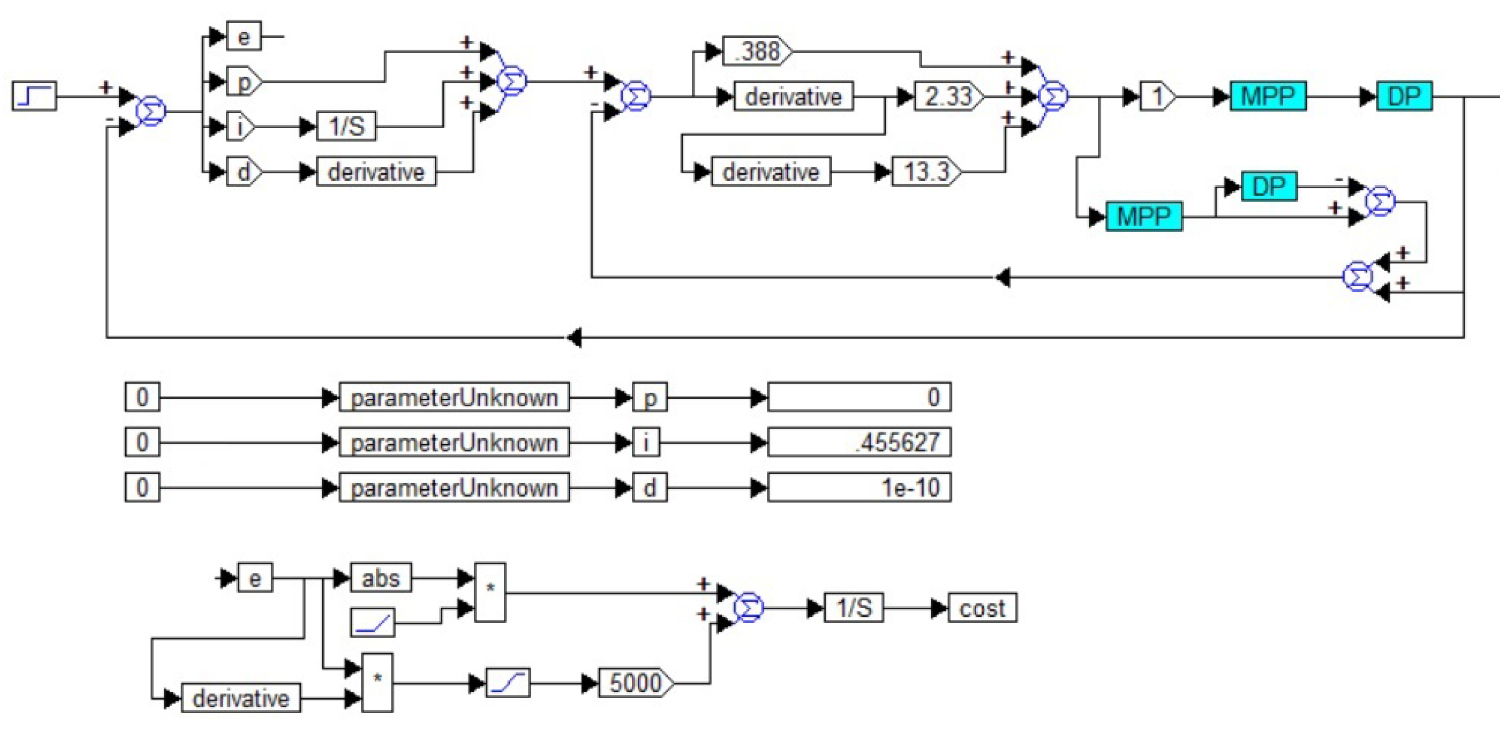
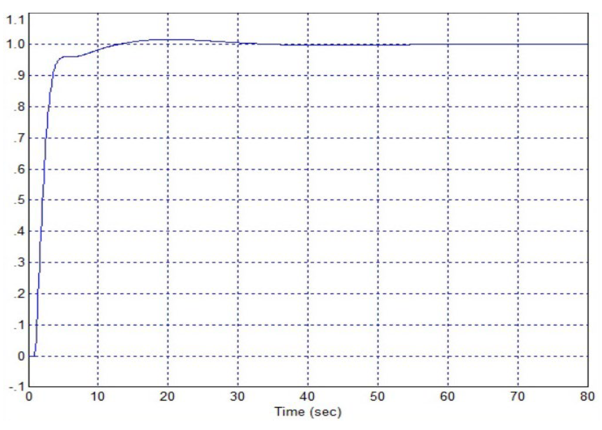
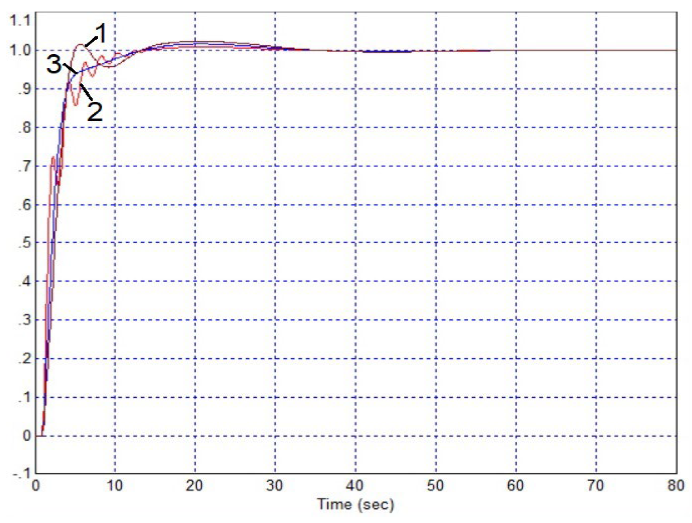
Figure 10.
Structure for modeling and optimization of a system with an external loop around a system with a PD2 controller and a Smith predictor.
Figure 10.
Structure for modeling and optimization of a system with an external loop around a system with a PD2 controller and a Smith predictor.
Figure 11.
Transient process in the system according to Figure 10.
Figure 11.
Transient process in the system according to Figure 10.
Figure 12.
Changes in the transient process in the system according to Figure 10 when the object’s gain changes: 1 – coefficient is reduced by 30%, 2 – original coefficient, 3 – coefficient is increased by 30%.
Figure 12.
Changes in the transient process in the system according to Figure 10 when the object’s gain changes: 1 – coefficient is reduced by 30%, 2 – original coefficient, 3 – coefficient is increased by 30%.
There is a lag element in the Smith predictor, as can be seen from the structure in Figure 10. For this reason, if the lag changes significantly, the controller calculated by this method using the wrong lag value may become unusable. However, when the delay changes within small limits, no more than 30% of the original value, the deterioration of the system is noticeable, but not fatal.
The proposed pseudo-local feedback controller is free from these disadvantages. Consider this method of designing a controller as applied to this problem.
3.2. Applying Pseudo-Local Feedback
Figure 13 shows a framework for modeling and optimizing a system with pseudo-local feedback and an external loop with a sequential PID controller. In this case, the coefficients in the pseudo-local PD2 controller are taken from the previous optimization result, and the coefficients of the sequential PID controller are obtained by the numerical optimization method. Overshoot in this case does not exceed 1%, the duration of the process can be estimated at 10 s, and if we do not take into account the process from overshoot within a deviation of 1%, then the process time can be considered equal to 5 s. If you use a PID 3 controller in a pseudo-local loop, as shown in Figure 14, then the system as a whole provides control with ideal quality, since there is no overshoot at all, the duration of the transient process is about 7 s.
The resulting system has the required robustness property. When the object gain increases by 30%, an overshoot of 4% occurs in the process, the duration of the process is 7 s, as shown in Figure 15, line 1, line 2 also shows the process at the initial value of this coefficient, and when the coefficient is reduced by 30%, the process remains without overshoot, but the duration of the process increases to 13 s.
Next, let us pay attention to the fact that in the pseudo-local contour in the minimum-phase part of the object model there is an ideal integrator. It is advisable to abandon the use of an ideal integrator, replacing it with an aperiodic link with the same amplitude-frequency characteristic in the region of medium and high frequencies, but having a limited gain in the region of low and zero frequencies, whereas for an ideal integrator this characteristic increases infinitely. This somewhat simplifies the regulator and ensures restoration of astatic control of the internal circuit. The final controller structure is shown in Figure 16, with the outer loop sequential controller coefficients re-optimized using a numerical optimization procedure, but they are not significantly different from the previously obtained values.
Finally, the transfer function of the sequential controller has the form:
The transfer function of the pseudo-local loop is:
This loop can be replaced by a sequential controller W1(s) based on the rule of equivalent transformation of the closed-loop transfer function:
After elementary transformations, we obtain the final form of this transfer function:
The final verification and refinement of this solution is that the coefficients in which there are more than three significant digits in the calculation are rounded to three significant digits and in the refined structure we additionally optimize the sequential PID controller.
Figure 17 shows the final structure with a single stabilization loop, in which the series controller is a series connection of a PID controller and a controller of type (14) with rounded coefficients. In this case, the transfer function of the PID controller has the form:
The transfer function of the second sequential link has the form:
The transient process does not have overshoot, the duration of the process is 7 s, the system has a single feedback loop, that is, the regulator is very simple in appearance, much simpler than all the regulators discussed above.
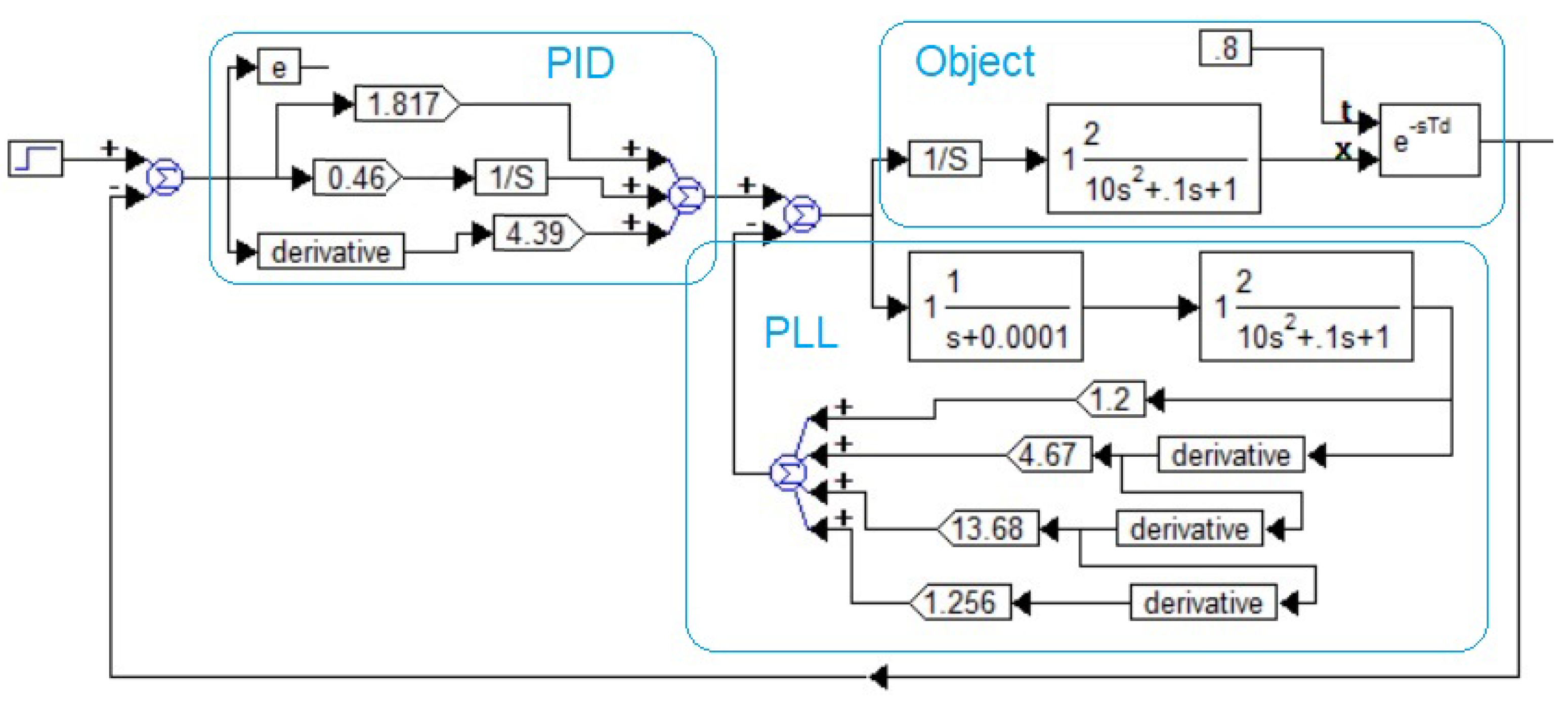
Figure 17.
Final system structure: PLL – pseudo-local loop, PID – serial PID controller.
The robustness properties when the gain changes by 30% and when the delay changes by 60% are confirmed by similar tests and the resulting graphs practically coincide with the graphs shown earlier in Figure 14 and Figure 15. For this reason, additional tests of the system were carried out with an even stronger deviation of the parameters of the object model.
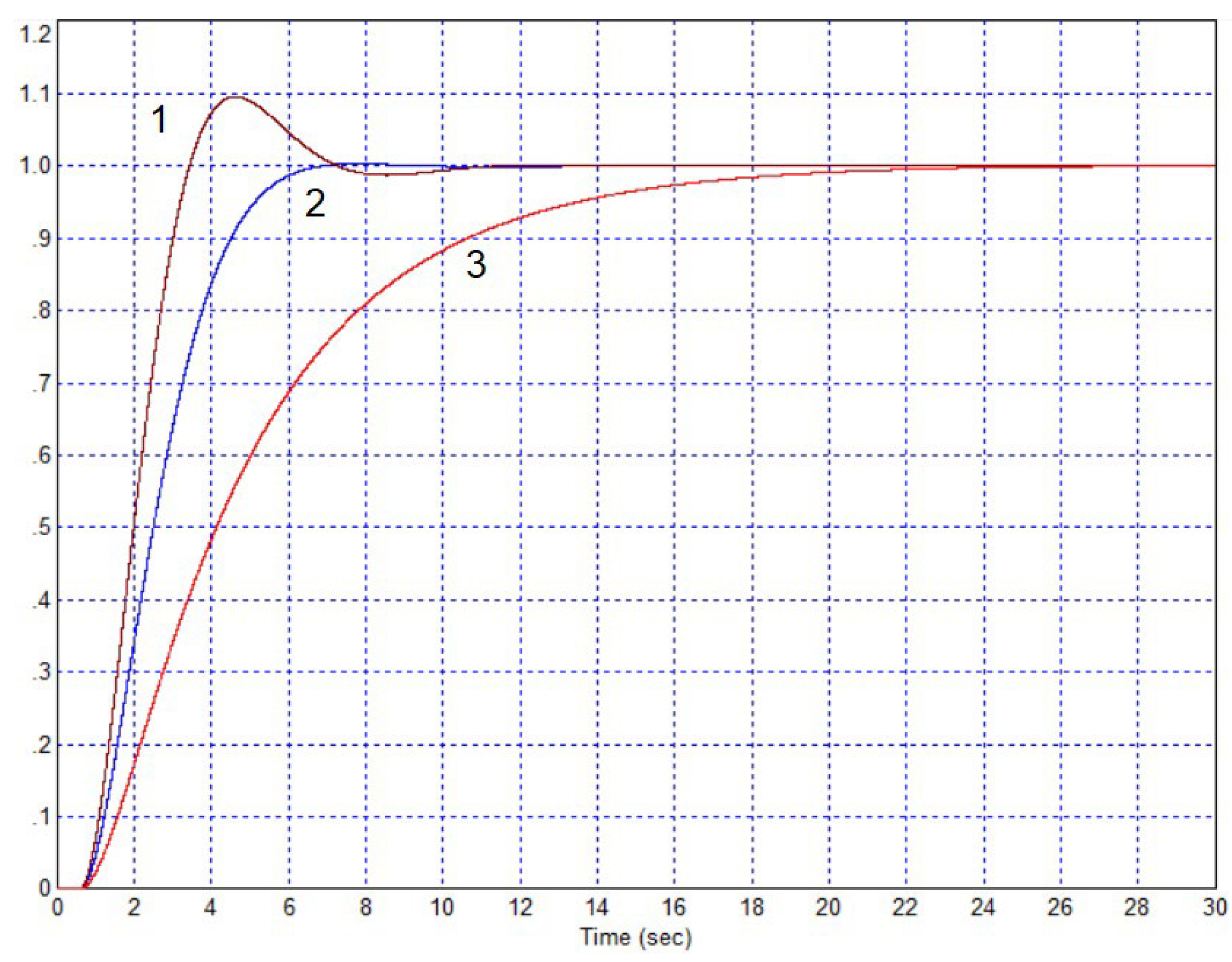
Figure 18 shows the result of the system with the delay change in the object model by 100%. When the delay is reduced to zero, the transient process retains its quality, reaching the deviation zone by 2% only slightly slower, but the duration of the transient process still remains short, about 10 s, and when the delay value is doubled, the overshoot reaches 10%, the duration of the process is at the level of 1 % remains the same, and the process duration at the 0.2% level is 14 s, as shown in Figure 18. Figure 19 shows the results with the object gain changed by 50%.
Based on the results of these complex tests, it can be stated that a method is proposed for controlling objects that are highly prone to oscillations due to the presence of a resonant link, an integrator and a delay link in their model. The effectiveness of the method has been confirmed by simulation; the structure of the controller is much simpler than a system with a Smith predictor.
4. Discussion
This article solved the problem of effective control of an object prone to oscillations due to the presence in its model of an oscillatory element in the form of a second-order filter with a high quality factor, a delay element for a significant amount of time commensurate with the time constant of this element, and an integrator. These elements are connected in series in the model. Since the object has an integrator, one could hope for sufficient efficiency of the PD2 controller, but the structure of such a sequential controller, which is effective for many other cases, turns out to be ineffective in this case. Even introducing the third derivative into the control channel does not solve the problem.
The use of the Smith predictor with subsequent numerical optimization of the controller coefficients has been demonstrated, which does not provide a sufficiently high quality of control. It is additionally proposed to provide control with higher quality using an external loop with a PID controller, the coefficients of which are calculated by numerical simulation. It is shown that in combination with all these methods the problem is solved with better quality, but the structure of the controller remains too complex. It is shown that when using a PID3 controller in the internal loop, if you use only the Smith predictor and the internal loop, control is provided with overshoot of no more than 9% and with a process duration of about 15 s; due to the external loop, overshoot is reduced to a value of 0.5%, duration the process is reduced to 10 s. If third-order differentiation is not used in the internal loop, then with a PID2 controller without an external loop it is possible to provide control with an overshoot of 11% and a process duration of 25 s, and with an external loop the overshoot is reduced to 1.5%, the process duration is about 15 s, the error becomes less than 0.1% after 35 s. The robustness of the resulting solution has been demonstrated, so in the case of changing the gain of the object model by 30% in both directions, the process remains of sufficiently high quality: overshoot does not exceed 1.5%, the process time is about 15 s, the time until the control error is reduced to a negligible value remains no more than 30 s.
5. Conclusions
It is proposed to use pseudo-local feedback, which gives a similar result with greater simplicity of the controller. It is also proposed to recalculate the pseudo-local controller through equivalent transformations, then round off the coefficients and again optimize the sequential PID controller. The resulting controller provides ideal control quality, since there is no overshoot, but the transition process in terms of the rate of reaching zero error is much faster than the exponential process.
The proposed method can be used to control objects that are highly prone to oscillations at a resonant frequency due to the presence of a resonant link in the object model and due to the presence of a delay link.
Author Contributions
All contribution is made by V.Z.
Funding
“This research was funded by government assignment”.
Data Availability Statement
Past and future data from these studies are available on the website https://www.scopus.com/authid/detail.uri?authorId=6602329136
Acknowledgments
The author thanks academician Sergei Bagaev for his support and approval of the research performed.
Conflicts of Interest
“The authors declare no conflict of interest.”
References
- So, G.-B. Design of Linear PID Controller for Pure Integrating Systems with Time Delay Using Direct Synthesis Method. Processes 2022, 10, 831. [Google Scholar] [CrossRef]
- He, J.; Su, S.; Wang, H.; Chen, F.; Yin, B. Online PID Tuning Strategy for Hydraulic Servo Control Systems via SAC-Based Deep Reinforcement Learning. Machines 2023, 11, 593. [Google Scholar] [CrossRef]
- Sozański, K. Low Cost PID Controller for Student Digital Control Laboratory Based on Arduino or STM32 Modules. Electronics 2023, 12, 3235. [Google Scholar] [CrossRef]
- Qu, S.; He, T.; Zhu, G. Model-Assisted Online Optimization of Gain-Scheduled PID Control Using NSGA-II Iterative Genetic Algorithm. Appl. Sci. 2023, 13, 6444. [Google Scholar] [CrossRef]
- Song, L.; Xu, C.; Hao, L.; Yao, J.; Guo, R. Research on PID Parameter Tuning and Optimization Based on SAC-Auto for USV Path Following. J. Mar. Sci. Eng. 2022, 10, 1847. [Google Scholar] [CrossRef]
- Vrančić, D.; Moura Oliveira, P.; Bisták, P.; Huba, M. Model-Free VRFT-Based Tuning Method for PID Controllers. Mathematics 2023, 11, 715. [Google Scholar] [CrossRef]
- Silaa, M.Y.; Barambones, O.; Bencherif, A. A Novel Adaptive PID Controller Design for a PEM Fuel Cell Using Stochastic Gradient Descent with Momentum Enhanced by Whale Optimizer. Electronics 2022, 11, 2610. [Google Scholar] [CrossRef]
- Zhang, M.-L.; Zhang, Y.-J.; He, X.-L.; Gao, Z.-J. Adaptive PID Control and Its Application Based on a Double-Layer BP Neural Network. Processes 2021, 9, 1475. [Google Scholar] [CrossRef]
- Cruz- Diaz, C.; del Muro-Cuéllar, B.; Duchén -Sánchez, G.; Márquez -Rubio, J. F.; Velasco-Villa, M. Observer-Based PID Control Strategy for the Stabilization of Delayed High Order Systems with up to Three Unstable Poles. Mathematics 2022, 10, 1399. [Google Scholar] [CrossRef]
- Arrieta, O.; Campos, D.; Rico- Azagra, J.; Gil- Martinez, M.; Rojas, J.D.; Vilanova, R. Model-Based Optimization Approach for PID Control of Pitch–Roll UAV Orientation. Mathematics 2023, 11, 3390. [Google Scholar] [CrossRef]
- Božek, P.; Nikitin, Y. The Development of an Optimally-Tuned PID Control for the Actuator of a Transport Robot. Actuators 2021, 10, 195. [Google Scholar] [CrossRef]
- Zishan, F.; Akbari, E.; Montoya, O.D.; Giral-Ramírez, D.A.; Molina-Cabrera, A. Efficient PID Control Design for Frequency Regulation in an Independent Microgrid Based on the Hybrid PSO-GSA Algorithm. Electronics 2022, 11, 3886. [Google Scholar] [CrossRef]
- Garrido, J.; Ruz, M.L.; Morilla, F.; Vázquez, F. Iterative Method for Tuning Multiloop PID Controllers Based on Single Loop Robustness Specifications in the Frequency Domain. Processes 2021, 9, 140. [Google Scholar] [CrossRef]
- Batiha, I.M.; Ababneh, O.Y.; Al-Nana, A.A.; Alshanti, W.G.; Alshorm, S.; Momani, S. A Numerical Implementation of Fractional-Order PID Controllers for Autonomous Vehicles. Axioms 2023, 12, 306. [Google Scholar] [CrossRef]
- İçmez, Y.; Can, M. S. Smith Predictor Controller Design Using the Direct Synthesis Method for Unstable Second-Order and Time-Delay Systems. Processes 2023, 11, 941. [Google Scholar] [CrossRef]
- Guo, X.; Shirkhani, M.; Ahmed, E.M. Machine-Learning-Based Improved Smith Predictive Control for MIMO Processes. Mathematics 2022, 10, 3696. [Google Scholar] [CrossRef]
- Baskys, A. Switched-Delay Smith Predictor for the Control of Plants with Response-Delay Asymmetry. Sensors 2023, 23, 258. [Google Scholar] [CrossRef]
- Li, M.; Xin, M.; Zhao, Z.; Wang, J.; Hu, X. Smith-Predictor-Based Design of Analytical PI-PD Control for Series Cascade Processes with Time Delay. Electronics 2023, 12, 4089. [Google Scholar] [CrossRef]
- Huba, M.; Bistak, P.; Vrancic, D. 2DOF IMC and Smith-Predictor-Based Control for Stabilized Unstable First Order Time Delayed Plants. Mathematics 2021, 9, 1064. [Google Scholar] [CrossRef]
- Song, M.; Liu, H.; Xu, Y.; Wang, D.; Huang, Y. Decoupling Adaptive Smith Prediction Model of Flatness Closed-Loop Control and Its Application. Processes 2020, 8, 895. [Google Scholar] [CrossRef]
- Pei, G.; Yu, M.; Xu, Y.; Ma, C.; Lai, H.; Chen, F.; Lin, H. An Improved PID Controller for the Compliant Constant-Force Actuator Based on BP Neural Network and Smith Predictor. Appl. Sci. 2021, 11, 2685. [Google Scholar] [CrossRef]
- Chuong, V.L.; Vu, T.N.L.; Truong, N.T.N.; Jung, J. H. An Analytical Design of Simplified Decoupling Smith Predictors for Multivariable Processes. Appl. Sci. 2019, 9, 2487. [Google Scholar] [CrossRef]
- Hu, X.; Tan, W.; Hou, G. Tuning of PID/PIDD2 Controllers for Second-Order Oscillatory Systems with Time Delays. Electronics 2023, 12, 3168. [Google Scholar] [CrossRef]
- Fawwaz, M.A.; Bingi, K.; Ibrahim, R.; Devan, P.A.M.; Prusty, B.R. Design of PIDD αController for Robust Performance of Process Plants. Algorithm 2023, Algorithm 16 and Algorithm 437. [CrossRef]
- VA Zhmud. Inadmissible Extensions of Protected Provisions in the Field of Automation: on the Control of Objects with Non-Square Transfer Functions. Automatics & Software Engineering. 2022, No. 1 (39). P.129 – 142. (In Russian). http://jurnal.nips.ru/sites/default/files/AaSI-1-2022-11.pdf.
- VA Zhmud, AV Liapidevskiy. The Design of the Feedback Systems by Means of the Modeling and Optimization in the Program VisSim 5.6/6.0 // Proc. Of The 30th IASTED Conference on Modelling, Identification, and Control ~ AsiaMIC 2010 ~November 24 – 26, 2010 Phuket, Thailand. P. 27–32.
- Zhmud, V. Designing of complete multi-channel PD-regulators by numerical optimization with simulation / V. Zhmud, L. Dimitrov // International Siberian conference on control and communications (SIBCON–2015): proc., Omsk, 21–23 May, 2015. – Omsk: IEEE, 2015. – Art. 129 (6 p.). ISBN 978-1-4799-7102-2. [CrossRef]
Figure 1.
Structure of the mathematical model of the object.
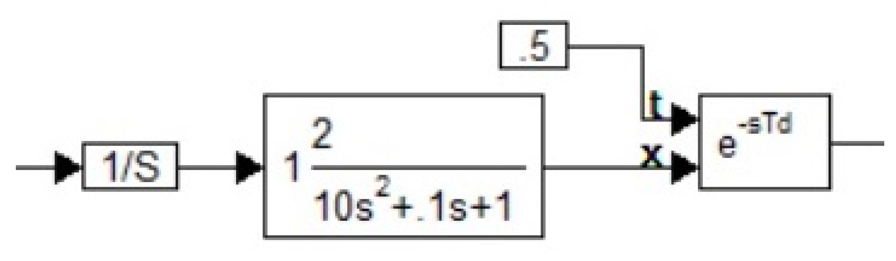
Figure 2.
Structure for numerical modeling of a system with an object (3) and a controller (2).
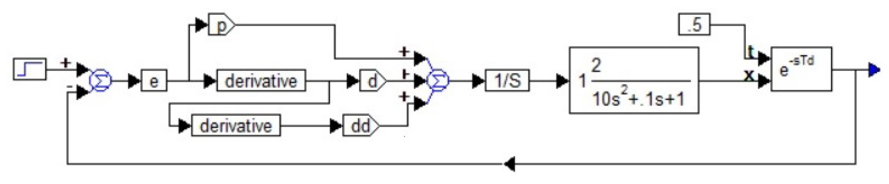
Figure 4.
Structure for modeling and optimization of a system with a PD3 controller and a Smith predictor using the cost function (5), optimization results are shown in numerical displays.
Figure 4.
Structure for modeling and optimization of a system with a PD3 controller and a Smith predictor using the cost function (5), optimization results are shown in numerical displays.
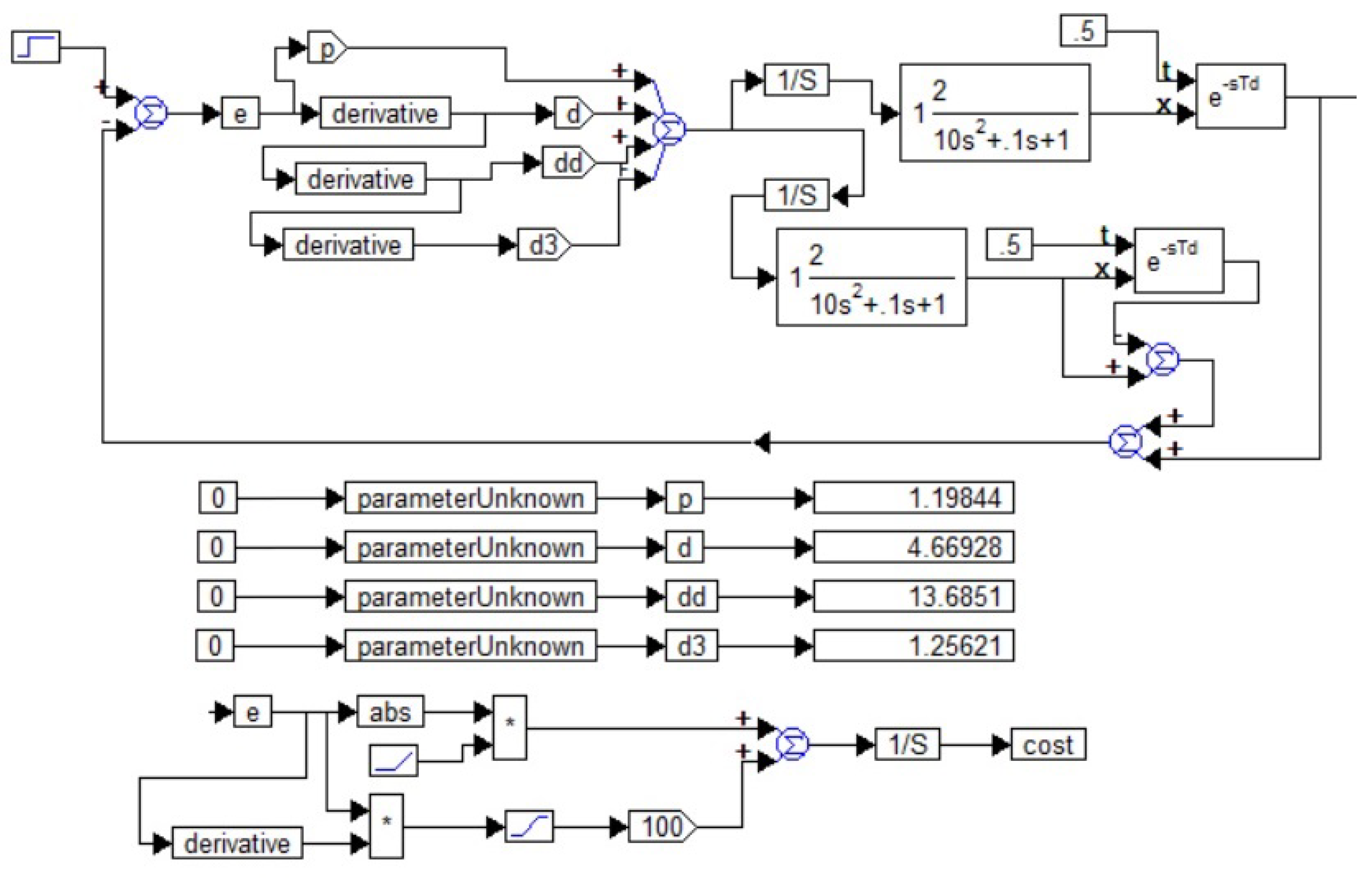
Figure 5.
Transient process in the system according to Figure 4.
Figure 5.
Transient process in the system according to Figure 4.
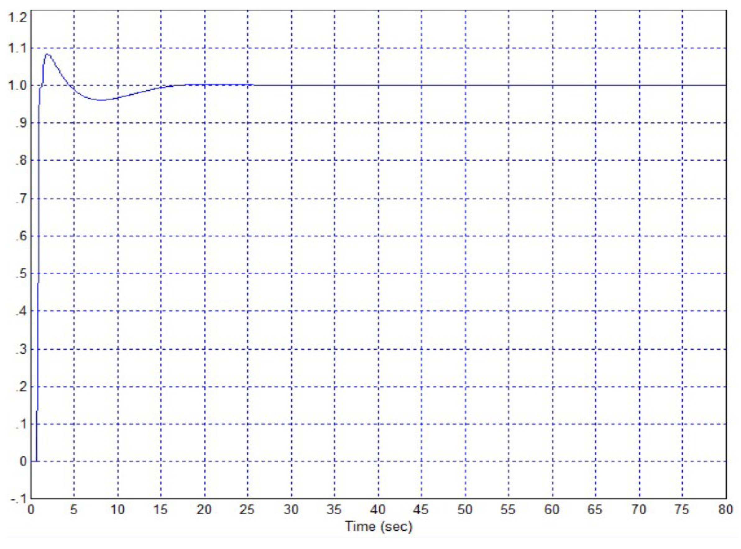
Figure 8.
Structure for modeling and optimization of a system with a PD2 controller and a Smith predictor.
Figure 8.
Structure for modeling and optimization of a system with a PD2 controller and a Smith predictor.
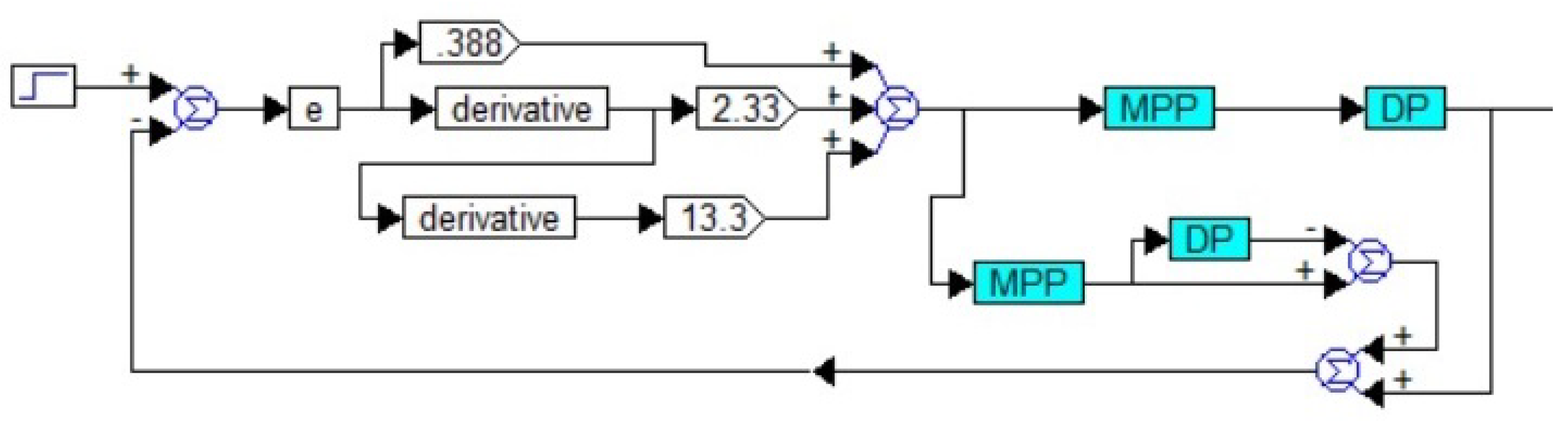
Figure 9.
Transient process in the system according to Figure 8.
Figure 9.
Transient process in the system according to Figure 8.
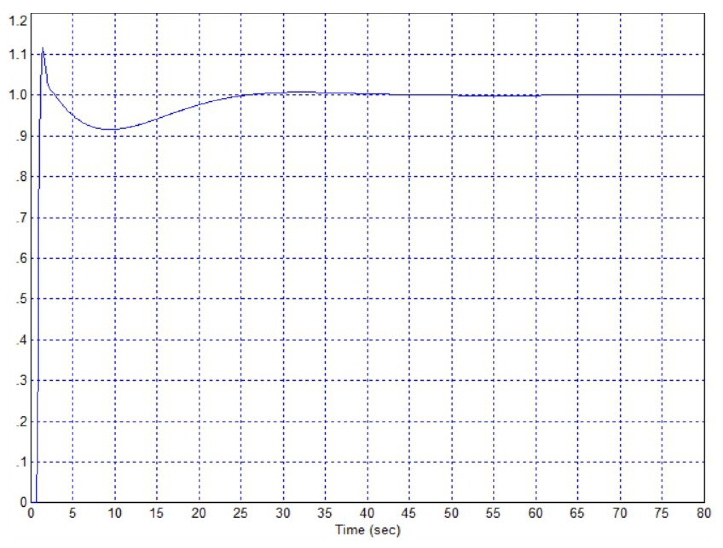
Figure 13.
Framework for modeling and optimizing a pseudo-local feedback system with a PID2 controller and an external loop with a sequential PID controller.
Figure 13.
Framework for modeling and optimizing a pseudo-local feedback system with a PID2 controller and an external loop with a sequential PID controller.

Figure 14.
Framework for modeling and optimization of a pseudo-local feedback system with a PID3 controller and an external loop with a sequential PID controller.
Figure 14.
Framework for modeling and optimization of a pseudo-local feedback system with a PID3 controller and an external loop with a sequential PID controller.
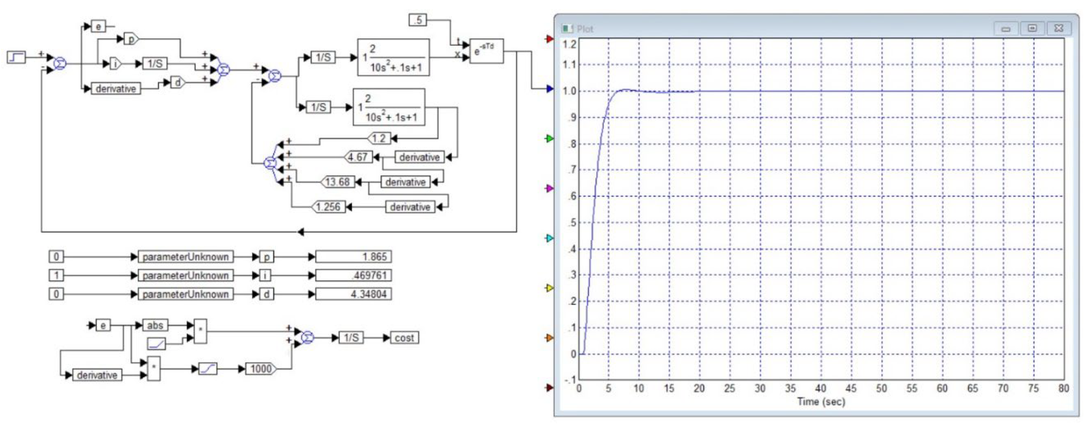
Figure 15.
Changes in the transient process in the system according to Figure 13 when the object’s gain coefficient changes: 1 – coefficient increased by 30%, 2 – original coefficient, 3 – coefficient reduced by 30%.
Figure 15.
Changes in the transient process in the system according to Figure 13 when the object’s gain coefficient changes: 1 – coefficient increased by 30%, 2 – original coefficient, 3 – coefficient reduced by 30%.
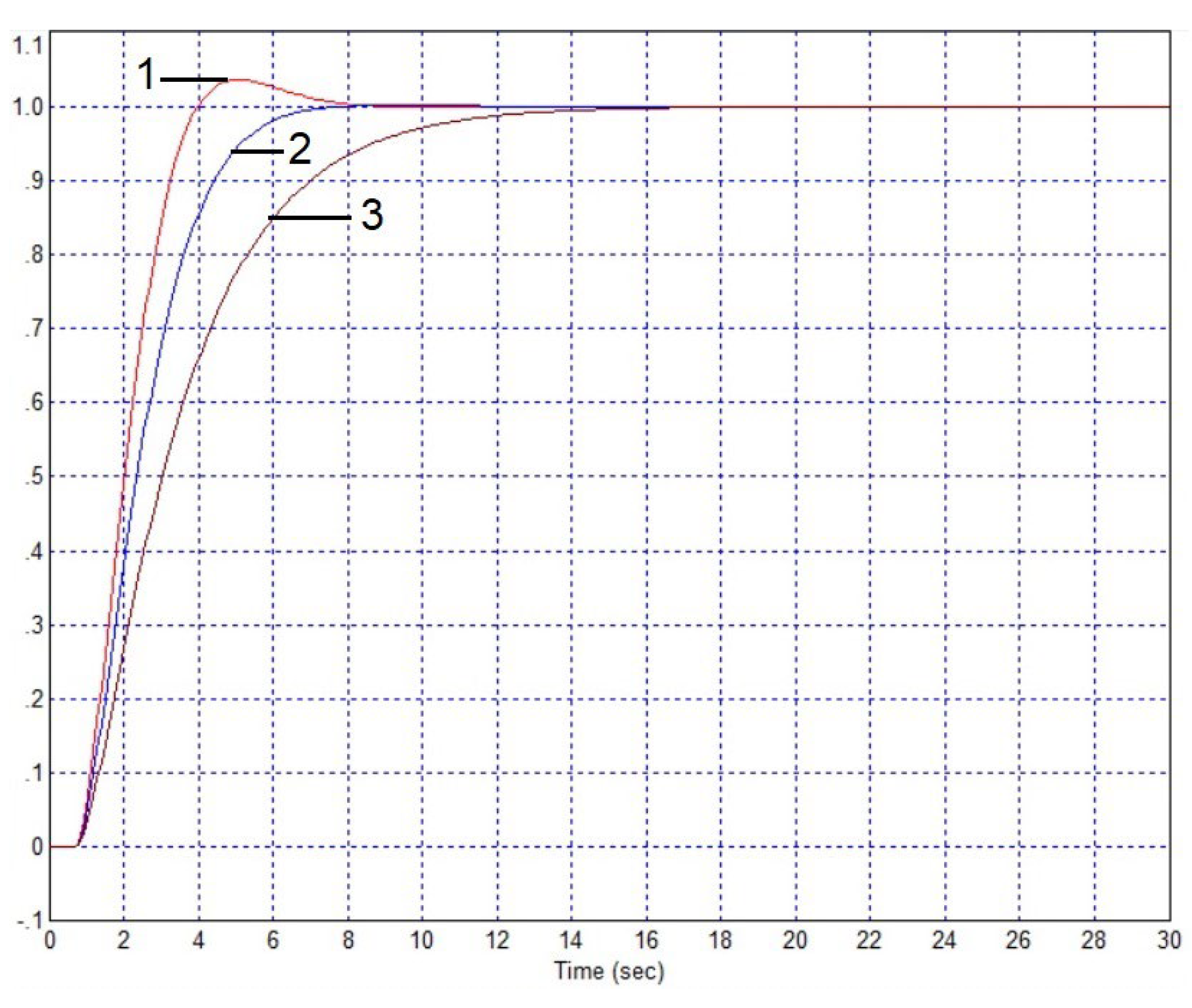
Figure 16.
Changes in the transient process in the system according to Figure 13 when the delay in the object model changes: 1 – delay is increased by 60%, 2 – initial value, 3 – delay is reduced by 60%.
Figure 16.
Changes in the transient process in the system according to Figure 13 when the delay in the object model changes: 1 – delay is increased by 60%, 2 – initial value, 3 – delay is reduced by 60%.
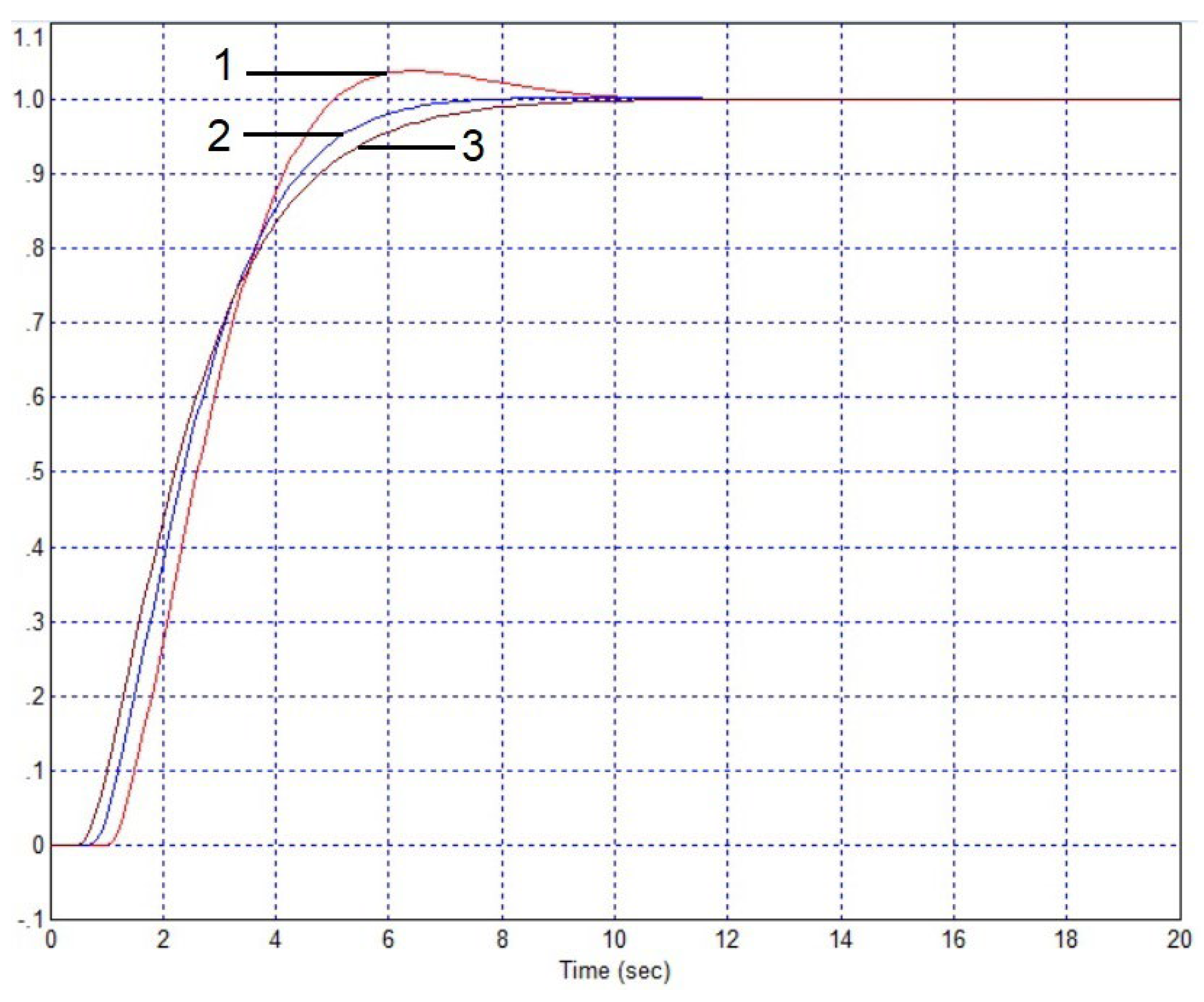
Figure 18.
Final structure of the system with a single loop and the resulting transient process.
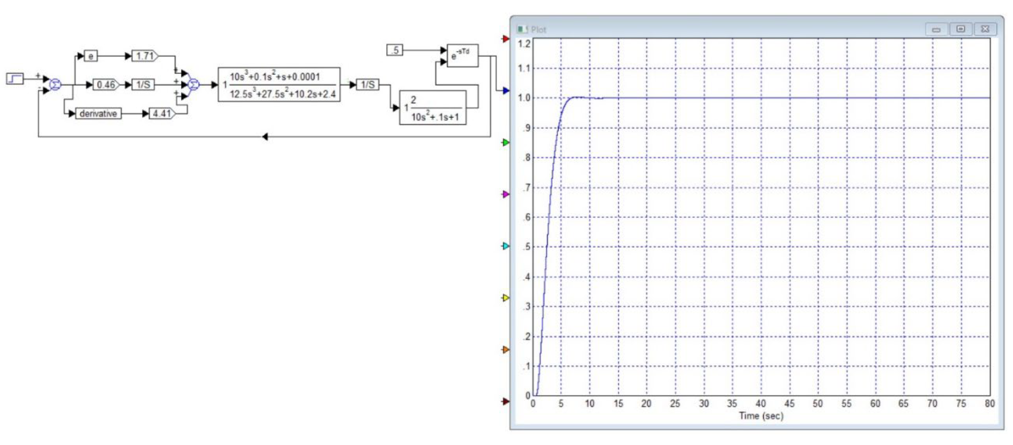
Figure 19.
Changes in the transient process in the system according to Figure 17 when the delay in the object model changes: 1 – delay is increased by 100%, 2 – initial value, 3 – delay is reduced by 100%.
Figure 19.
Changes in the transient process in the system according to Figure 17 when the delay in the object model changes: 1 – delay is increased by 100%, 2 – initial value, 3 – delay is reduced by 100%.
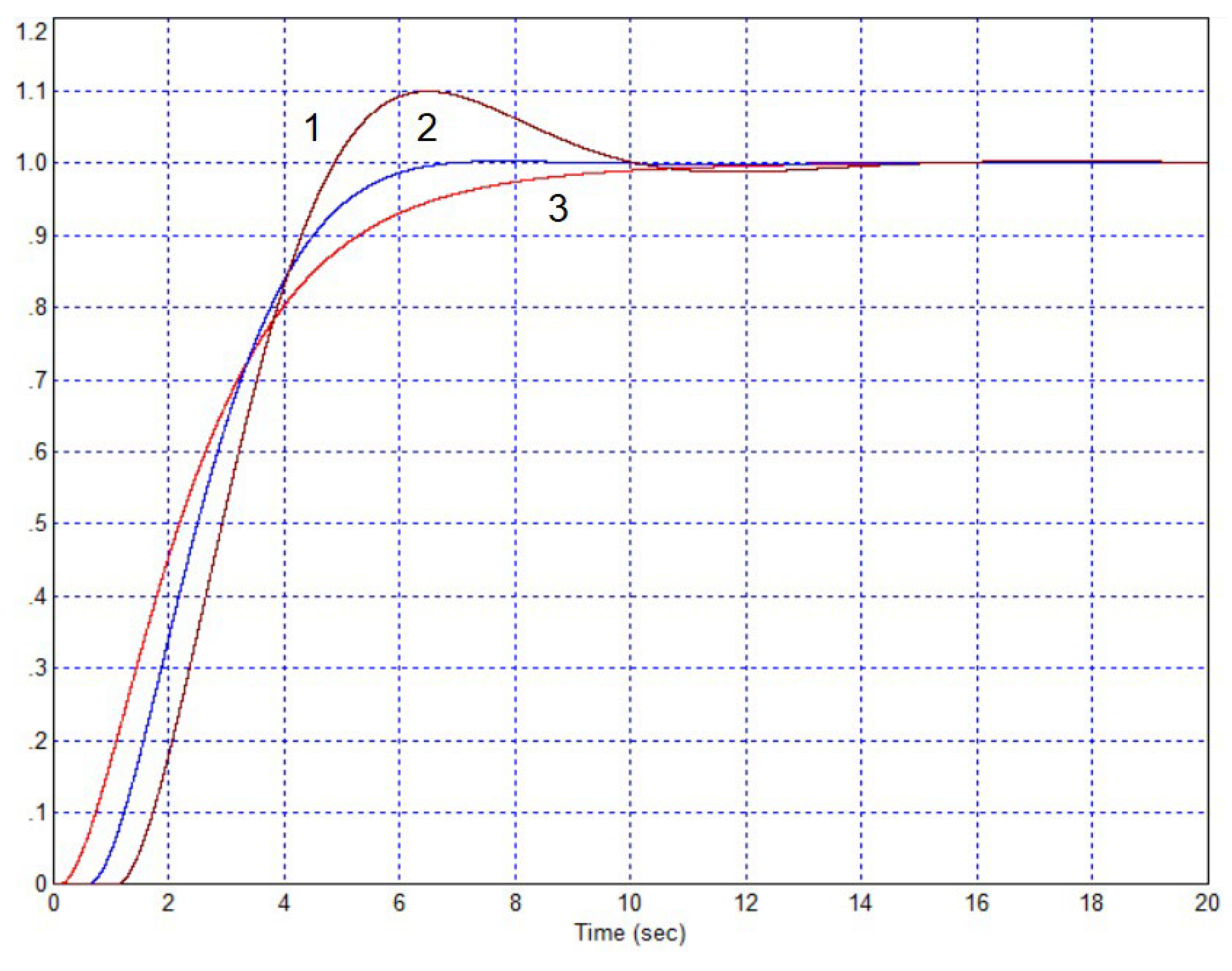
Figure 20.
Changes in the transient process in the system according to Figure 18 when the object’s gain changes: 1 – coefficient increased by 50%, 2 – original coefficient, 3 – coefficient reduced by 50%.
Figure 20.
Changes in the transient process in the system according to Figure 18 when the object’s gain changes: 1 – coefficient increased by 50%, 2 – original coefficient, 3 – coefficient reduced by 50%.
Disclaimer/Publisher’s Note: The statements, opinions and data contained in all publications are solely those of the individual author(s) and contributor(s) and not of MDPI and/or the editor(s). MDPI and/or the editor(s) disclaim responsibility for any injury to people or property resulting from any ideas, methods, instructions or products referred to in the content. |
© 2024 by the authors. Licensee MDPI, Basel, Switzerland. This article is an open access article distributed under the terms and conditions of the Creative Commons Attribution (CC BY) license (http://creativecommons.org/licenses/by/4.0/).
Copyright: This open access article is published under a Creative Commons CC BY 4.0 license, which permit the free download, distribution, and reuse, provided that the author and preprint are cited in any reuse.


