Submitted:
06 April 2024
Posted:
09 April 2024
You are already at the latest version
Abstract
: This paper presents a comparison between direct integer orders or classical model reference adaptive control (IO-DMRAC) versus its fractional orders counterpart (FO-DMRAC) applied to the F-16 aircraft longitudinal model pitch rate control. A substantial improvement is achieved when using fractional order adaptive control, since, in addition to performance indices, such as Integral Square-Error criterion (ISE) and Integral Square-Input criterion (ISU) being lower, the oscillations of the system output (pitch rate) in the transient period, are eliminated. Moreover, it is the first attempt in literature of adaptive control that a FO-DMRAC is applied to the pitch rate control of an aircraft. A F-16 short-period model, whose relative degree is equal to 1 (n^*=1) is analyzed by mean of simulations with good results. A FO-DMRAC is designed, for a specific operating flight conditions and compared with its IO-DMRAC counterpart. Furthermore, the boundedness of all signals, including the internal ones ω(t) are assured.
Keywords:
Fractional order adaptive control
; smoother output signal
; Particle Swarm Optimization (PSO) algorithm.
1. Introduction
The pitch rate control of an aircraft (see Figure 2.1 for angles meaning) is the main system for tracking of a target by means of a combat aircraft and landing approach [1]. In addition, the pitch rate can be useful for estimating the attitude or pitch angle of an airplane because the pitch angle is the integral of the pitch rate. Therefore, is important to design a well-suited control system. In this work, we compare the classical or integer order direct model reference adaptive control (IO-DMRAC) with its fractional order counterparts (FO-DMRAC). The mathematical F-16 longitudinal model used in this paper is a second-order one [2] which considers the short-period oscillations mode neglecting the phugoid mode (large period oscillations) because the first mode (high-frequency oscillation), is more difficult to control by the pilot. Our interest is to show the lack of oscillation during the transient period using FO-DMRAC than the classical or integer order direct model reference adaptive controller (IO-DMRAC).
Very few adaptive control attempts are made for controlling the pitch rate of an aircraft, whose adaptive laws are of FO, not to mention any.
In [2], the longitudinal control of an F-16 is analyzed using a combined MRAC control technique.
By the other hand, small planes basically use PID controllers because of the easy implementation [3,4,5,6,7,8]. The main disadvantage is that PID controllers lack adaptation capabilities in case of plant parametric variations, because of the PID control parameters are constants, but an aircraft flight dynamic is variant.
In [9] a MRAC approach for the control of the longitudinal model of an F-15 aircraft is used and the only fractional term, is a filter that approximate the plant model. Moreover, additional blocks are added doing the implementation more complex.
Finally, the paper is structured as follows. In Section 2, the F-16 aircraft model is presented for a specific flight condition (at sea level) [2]. Section 3 shows the implementation of the DMRAC control system. In Section 4, basic concepts of FO calculus are shown that will be used in this comparative analysis. Also, we make use of a lemma that relax some stability condition, which was used in the longitudinal pitch angle control of a civil airplane [10]. The simulation results are presented in Section 5. Finally, the conclusion of this work is presented in Section 6.
2. Longitudinal Model and Flight Conditions
The aircraft model considers a straight and level flight condition [2]. Figure 1 shows the main angles involved for the study of longitudinal airplane models and control.
where θ is the pitch angle, γ is the flight path angle, V is the wind speed relative to the aircraft and α is the angle of attack (AoA).
A simple model, considering the longitudinal short period can be written in matrix form as [2]
where is the pitch rate (output), is the elevator deflection angle (input), V is the air trimmed speed, and are the partial derivatives of the aerodynamic vertical force and the pitch moment with respect to respectively. The coefficients matrix values of Equation (1) were taken from [2].
Table 1 shows the trimmed values used in this model.
Replacing the numeriacl values to Equation (1) we obtain
where and are the input and output system respectively.
Then, the transfer function of interest will be
Therefore, according to Equation (2), the transfer function , imposing null initial conditions, has the form
where , , and .
Then, the transfer function, between the pitch rate (the output) and (the input), is given by
or equivalently,
which is a second order () transfer function whose relative degree is equal to 1 (). The high frequency plant gain . Also, and are the plant numerator and denominator respectively.
3. Control Model System
Figure 2 shows a general block diagram of the DMRAC control system, in which the control parameters and and , are adjusted adaptively to keep the output control error as small as possible.
Figure 3 shows the Simulink DMRAC block diagram implemented for the simulations analysis. Also, the well-known DMRAC controller block diagram can be seen in Figure 4 [13]. The model transfer function was chosen as . One could choose another transfer function ( for instance), nevertheless, because we want a fast response, we used .
4. Controller Designs
For the sake of completeness, the adaptive DMRAC algorithm for plants whose relative degree 1 , is given in the next sub-section. A detailed explanation of the algorithm can be found in [13].
4.1. DMRAC Algorithm
In the DMRAC approach, the asymptotic convergence of the control parameters, to the ideal ones, are not relevant, making the implementation simpler since the identification block is avoided [13].
Therefore, the DMRAC control scheme of a linear plant of order , with relative degree equal 1 is shown in Figure 4, where only the output error is accessible (Adaptive Error Model Type 3) but not the whole state error vector (Error Model Type 2), in which case, the analysis for determining stability conditions is simpler [13].
Therefore, in this case (), the control law is given by
and is the controller parameters vector, is the auxiliary signals vector, and is the order of the plant.
are the parameters error vector controller.
are the ideal controller parameters.
The auxiliary signals are defined by
where and . is any arbitrary stable and controllable pair, with a Hurwitz matrix.
For simplicity, we choose in the controllable canonical form. Furthermore, when , the adaptive control parameters laws adjustment is chosen as:
The output control error can also be expressed as , where (the reference model) is a strictly positive real transfer function and we can derivate the same adaptive control laws as above.
It supposed that we know the sign of the high frequency gain and . Therefore, the adaptive laws can be simplified to
We can also aggregate adaptive gains to manage the speed of converge of the control parameters where . That to say, the adaptive gains can be different among them. Then, the more general adjusted adaptive laws can be re-written as
4. Fractional Calculus Preliminaries
In what follows, by no means exhaustive, we present some basic definitions of the fractional order Integral and derivative respectively [14,15]
Definition 1
[14]: The Riemann-Liouville fractional integral of order of a function is defined by
Definition 2
[14]: Let and . The Caputo fractional derivative of order of a function is defined as
Theorem 1:
Let the state errorand the output errorbe represented by Equation (11),
- a)
- The parametric error , the state error and the output error remain bounded for all time.
- b)
- Moreover, if the auxiliary signal is bounded, then and also remain bounded.
- c)
- The mean value of the squared norm of the state error is ,
or equivalently , where means that the speed of converges to zero is higher than . The demonstration of this theorem is available in [19].
From Theorem 1, since with a constant vector, then, the control error also will be .
If (c) holds, it must also hold for the mean value of the square norm of , since with a vector whose components are constants.
The next lemma (Lemma 2), relax the hypothesis (b) imposed from Theorem 1. A proof of this lemma can be found in [10].
Lemma 2:
Let us consider an order linear system of relative degree whose fractional adaptive laws are given by
Furthermore, as the auxiliary signal is bounded and because of Theorem 1 guarantees (c), then the squared norm of the output error , also tend to 0 as t tends to . Therefore, the stability of the proposed FO-DMRAC is guaranteed.
4.1. FO-DMRAC Algorithm
When , the only equation that change in the case of the FO-DMRAC algorithm, is the control parameter adaptive law (remember that the plant and the error equation are of integer order), therefore, in the classical case or IO-DMRAC, the adaptive law is given by
On the other hand, for the FO-DMRAC case, the adaptive law become
where (see Equation 7), therefore, the .
Finally, the control is given by
5. Simulations
Simulations were performed using Matlab & Simulink [20]. Furthermore, the pitch rate initial conditions were set to zero for both cases (integer and fractional order controllers).
Table 2 shows a detailed setting of the FO-DMRAC and IO-DMRAC controllers for simulations purpose.
there and are diagonal matrices of adaptive gains. For the implementation of the fractional adaptive laws, the NID block based on the Oustaloup method were used [21,22].
5.1. IO-DMRAC v/s FO-DMRAC using PSO Algorithm
In this section, we compare the simulations results of using FO-DMRAC versus the classical or IO-DMRAC controller. Also, in both cases, we use the Particle Swarm Optimization (PSO) technique [23] assuring the best behavior for both cases. The numbers of particles used were 50 considering 50 iterations. Of course, any other optimization technic can be used to determine the adaptive gains and derivative orders .
5.2. Simulation Controller Results
The most important objective is minimizing the control error, therefore, the objective function used to be optimized was defined as
where is the control error, is a weighted parameter and the reference input signal is the unit step.
Remark 1.
Equation 17 was chosen as the objective function (ISE index) which is a simple index but in the case of a combat aircraft, it is a good election since the most important issue is to minimize the control error as fast as possible in contrast with having minimum control effort or fuel efficiency. Nevertheless, it should not be forgotten that the objective function can be chosen by the designer.
Figure 5 shows the objective function using the PSO algorithm versus the number of iterations.
The optimal parameters values obtained for the IO-DMRAC case were
In the same way, Figure 6 shows the evolution of the objective function for the FO-DMRAC case.
Therefore, the optimal parameters obtained, for the FO-DMRAC case, were
From Figure 5 and Figure 6, it can be observed a faster convergence rate to a stable value of lower magnitude of the objective function in the FO case (Figure 6) compared to the IO one (Figure 5). Therefore, a better controller system behavior could be expected for the FO case.
Figure 7 shows the behavior of both controllers. The reference signal (blue color) is depicted besides the outputs of the controlled systems. It is evident the better behavior of the Fractional Order controller (green color signal) which output signal is almost identical to the reference model signal without oscillations. In contrast, the Integer Order controller case (red color signal) present an evident oscillatory behavior during the transient period.
Figure 8 and Figure 9 show the control effort and control error respectively during the transient period for both cases (IO and FO controllers). As it can be seen, in the IO case, the control effort and the control output error present an oscillatory behavior in contrast to the FO case, which is smoother.
Table 3 shows the optimal values of the objective function for both controller’s case.
Referring to Table 3, it is evident that employing FO-DMRAC results in superior performance compared to the IO-DMRAC approach, as evidenced by the smaller objective function .
It is noteworthy that both controllers, the integer, and fractional ones, share the same structure, namely the classical model reference structure.
6. Conclusions
The main result of this comparative study between integer order (IO-DMRAC) and fractional order (FO-DMRAC) adaptive controllers, is the better performance achieved by the FO controller in contrast with the its IO counterpart, because the oscillations during the transient period of the pitch rate output, were eliminated without sacrificing much, the rest of the controller design parameters as rise time and settling time for noun some. Moreover, the control effort in the FO controller case was lower and smoother than its IO counterpart.
Also, the simulation results allow us to verify, as assured by Lemma 2, the boundedness of all the signals, including the internal ones in the FO-DMRAC implementation.
Further, as said before, it is the first time that a FO-DCARM pitch control is applied to an aircraft whose model is of integer order (F-16 longitudinal short-period model) and the adaptive laws are of fractional ones.
Finally, the asymptotic stability of the FO-DMRAC has been shown by means of simulations, (Figure 7), nevertheless, the theoretical proof is still a pending issue.
Acknowledgments
The research presented in this paper has been funded by CONICYT-Chile, under grant FONDECYT 1210031 and Advanced Center for Electrical and Electronic Engi neering, AC3E, Basal Project FB0008, ANID.
References
- Exprasit Promtum, Sridhar Seshagiri. Sliding mode control of pitch-rate of an F-16 aircraft. Proceeding of the 17th World Congress, The International Federation of Automatic Control, Seoul, Korea, -11, 2008. 6 July.
- Lavretsky, E. Combined/Composite Model Reference Adaptive Control. IEEE Trans. Autom. Control. 2009, 54, 2692–2697. [Google Scholar] [CrossRef]
- Seckel E, Stability and control of airplane and helicopters. Department of Aeronautical Engineering. The James Forrestal Research Center School of Engineering and Applied Science, Princeton University. New Jersey, 1964.
- Sheng Shouzhao, Sun Chenwu, Duan Haibin, Jiang Xiaoliang, Zhu Yansong, Longitudinal and Lateral Adaptive Flight Control Design for an Unmanned Helicopter with Coaxial Rotor and Ducted Fan, 2014.
- Roskam, J. , Airplane flight dynamics and automatic flight controls. Part 2. Roskam Aviation and Engineering Corporation, 1995.
- Analysis of autopilot system, integrated with modelling and comparison of different controllers with the system, Bharat Singh,Shabana Urooj &Sudhakar Singh. Pages 1059-1068, Apr 2020.
- Aircraft Pitch Control using PID Controller. M. Angelin Ponrani; A. Kirthini Godweena, International Conference on System, Computation, Automation and Networking (ICSCAN), IEEE Conference paper, 2021.
- Position Control in Simulated Airplanes.
- Ynineb, A.R.; Ladaci, S. MRAC Adaptive Control Design for an F15 Aircraft Pitch Angular Motion Using Dynamics Inversion and Fractional-Order Filtering. Int. J. Robot. Control. Syst. 2022, 2, 240–252. [Google Scholar] [CrossRef]
- Benavides, G.E.C.; Duarte-Mermoud, M.A.; Orchard, M.E.; Travieso-Torres, J.C. Pitch Angle Control of an Airplane Using Fractional Order Direct Model Reference Adaptive Controllers. Fractal Fract. 2023, 7, 342. [Google Scholar] [CrossRef]
- High angle of attack flight characteristics of a small UAV with a variable-size vertical tail. Baron Johnson. Thesis presented to the graduate school of the University of Florida, 2009.
- Stevens, B.L.; Lewis, F.L. Aircraft Control and Simulation. Aircr. Eng. Aerosp. Technol. 2004, 76. [Google Scholar] [CrossRef]
- K. S. Narendra and A. M. Annaswamy, Stable Adaptive Systems. Dover Publications Inc., 2005.
- Kilbas, H. Srivastava, and J. Trujillo. Theory, and applications of fractional differential equations. Elsevier, 2006.
- K. Diethelem. The Analysis of Fractional Differential Equations. Springer-Verlag, Berlin-Heidelberg, 2010.
- Duarte-Mermoud, M.A.; Aguila-Camacho, N.; Gallegos, J.A.; Castro-Linares, R. Using general quadratic Lyapunov functions to prove Lyapunov uniform stability for fractional order systems. Commun. Nonlinear Sci. Numer. Simul. 2015, 22, 650–659. [Google Scholar] [CrossRef]
- N. Aguila-Camacho, M.A. N. Aguila-Camacho, M.A. Duarte-Mermoud, J.A. Gallegos. Lyapunov Functions for Fractional Order Systems. Communications in Nonlinear Science and Numerical Simulation, Vol. 19, No. 9, 2014, pp. 2951–2957, 2014.
- Aguila-Camacho, N.; Duarte-Mermoud, M.A. Boundedness of the solutions for certain classes of fractional differential equations with application to adaptive systems. ISA Trans. 2016, 60, 82–88. [Google Scholar] [CrossRef] [PubMed]
- Aguila-Camacho, N.; Gallegos, J.; Duarte-Mermoud, M.A. Analysis of Fractional Order Error Models in Adaptive Systems: Mixed Order Cases. Fract. Calc. Appl. Anal. 2019, 22, 1113–1132. [Google Scholar] [CrossRef]
- The Math Works Inc. Control system toolbox user's guide. 1998. http:\\www.mathworks.com.
- Valerio, D. & da Costa, “Ninteger: a non-integer control toolbox for matlab”. In Fractional Derivatives and Applications. OIFAC, Bordeaux, France, 2004.
- V. Sabatier, J. V. Sabatier, J., Aoun, M, Oustaloup, A., Gregoire, G., Ragot, E., & Roy, P. Fractional system identification for lead acid battery state of charge estimation. Signal Processing, 86, 2645-2657, 2006.
- Maurice Clerc. Particle Swarm Optimization. ISTE Ltd., 2006.
Figure 1.
Longitudinal aircraft angles (figure uploaded by Baron Johnson [11]).
Figure 1.
Longitudinal aircraft angles (figure uploaded by Baron Johnson [11]).
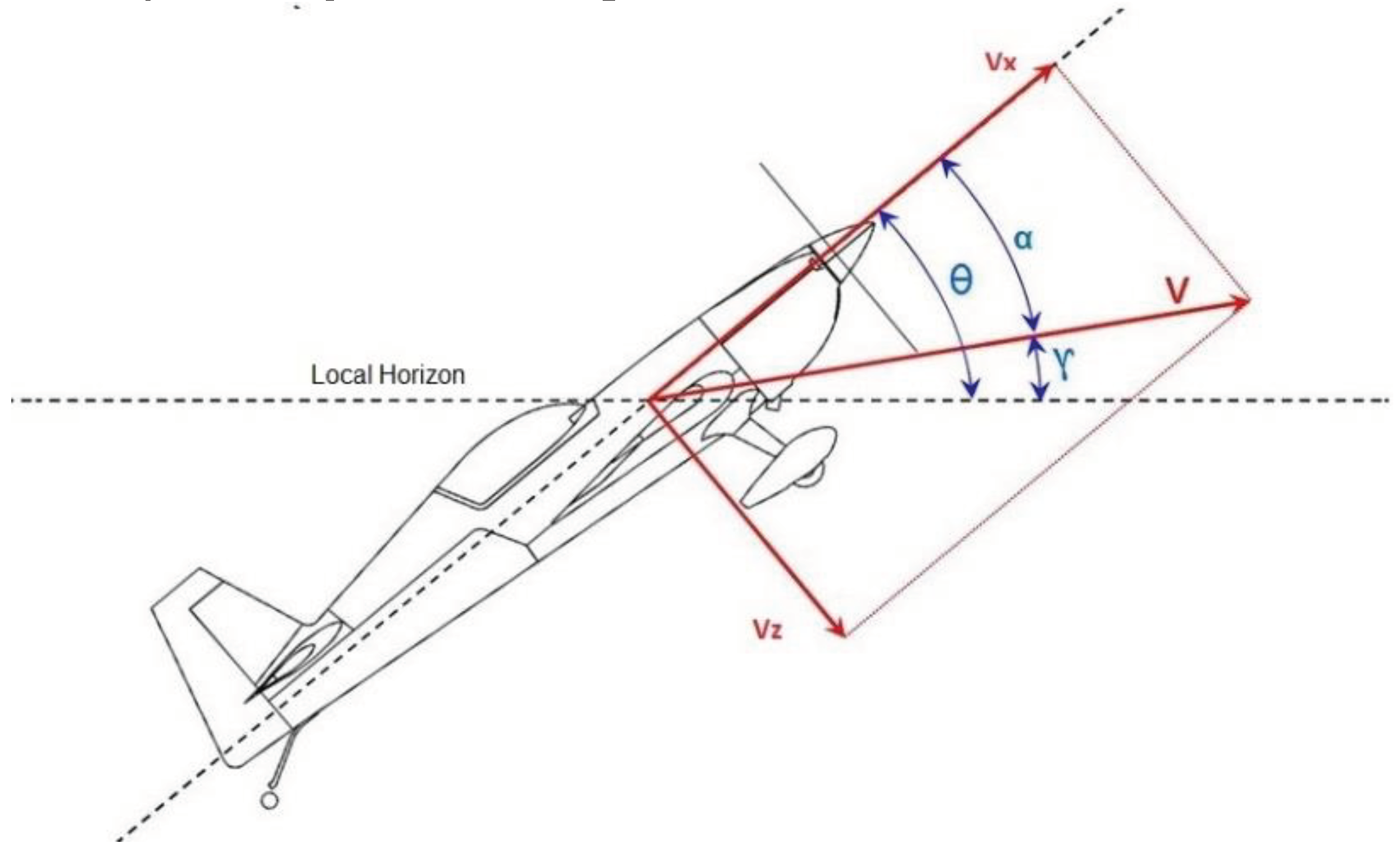
Figure 2.
DMRAC Block diagram.
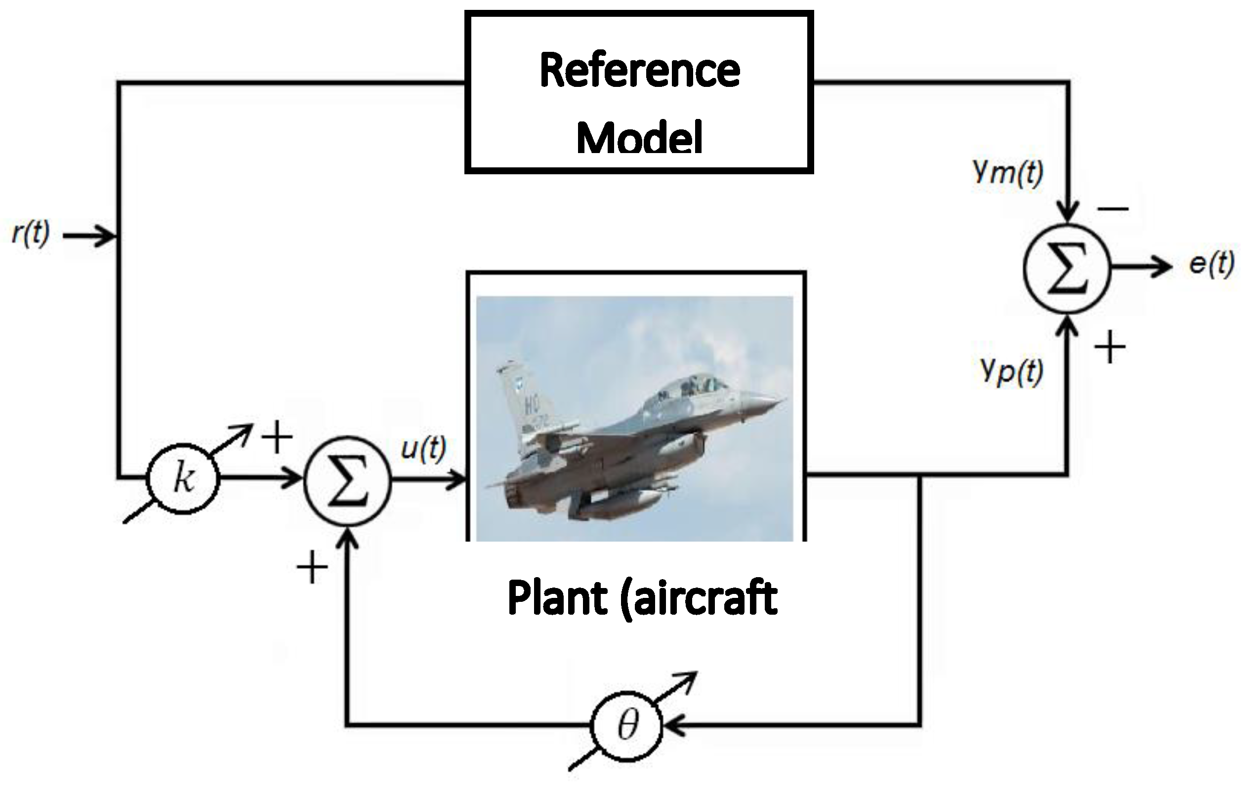
Figure 3.
Simulink DMRAC control block diagram of the F-16 short-period mode.
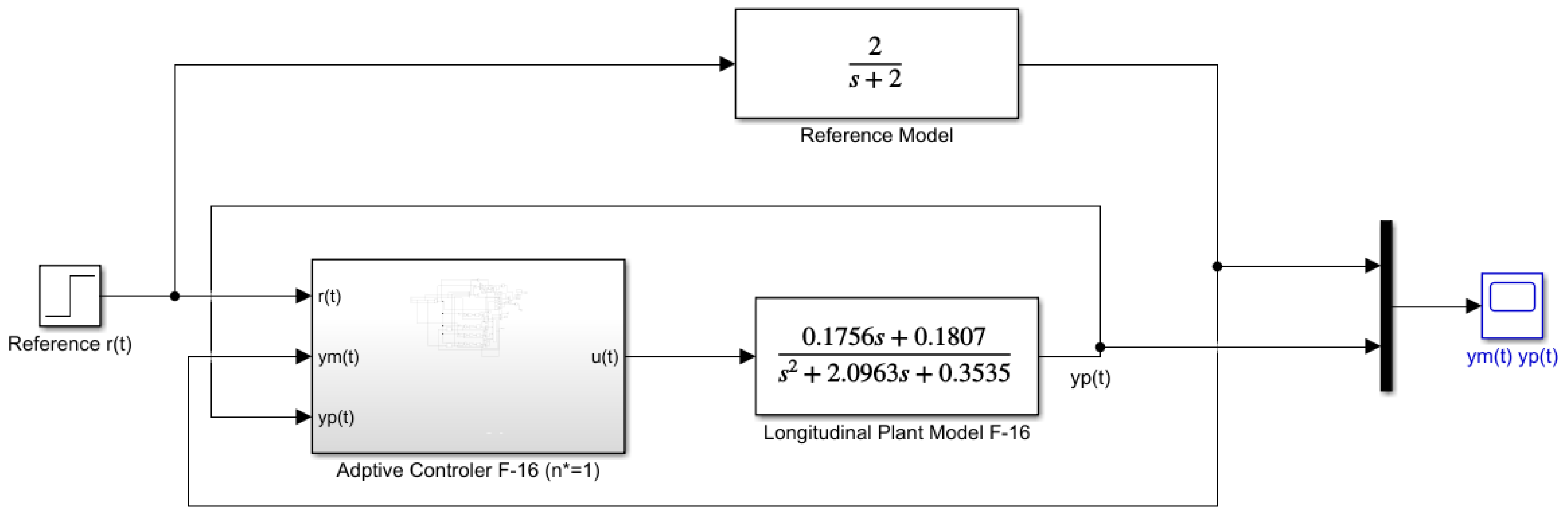
Figure 4.
DMRAC block diagram for Plant relative degree is 1 () the case.
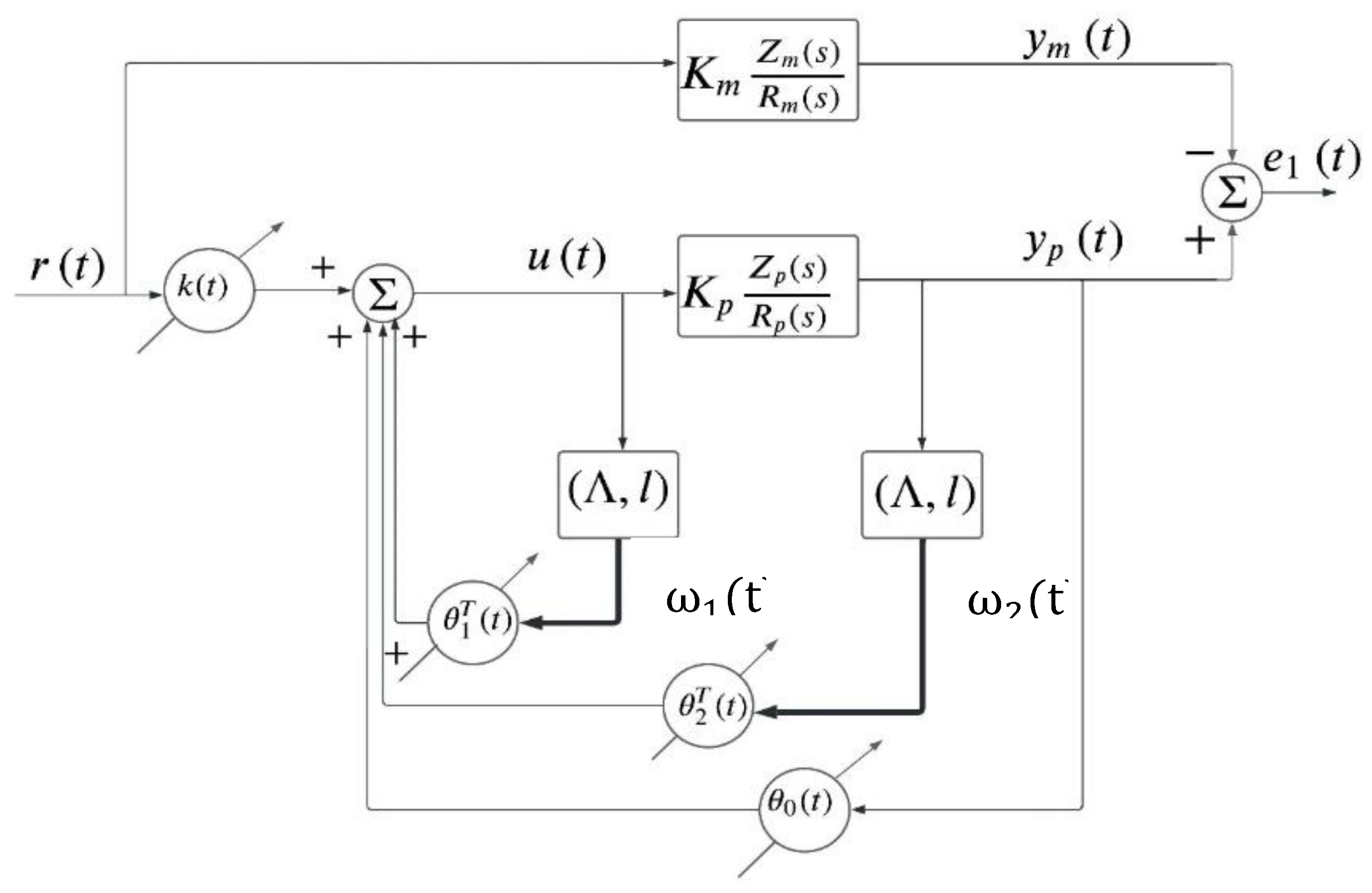
Figure 5.
Objective function evolution using PSO optimization algorithm for the MRAC integer order case controller.
Figure 5.
Objective function evolution using PSO optimization algorithm for the MRAC integer order case controller.
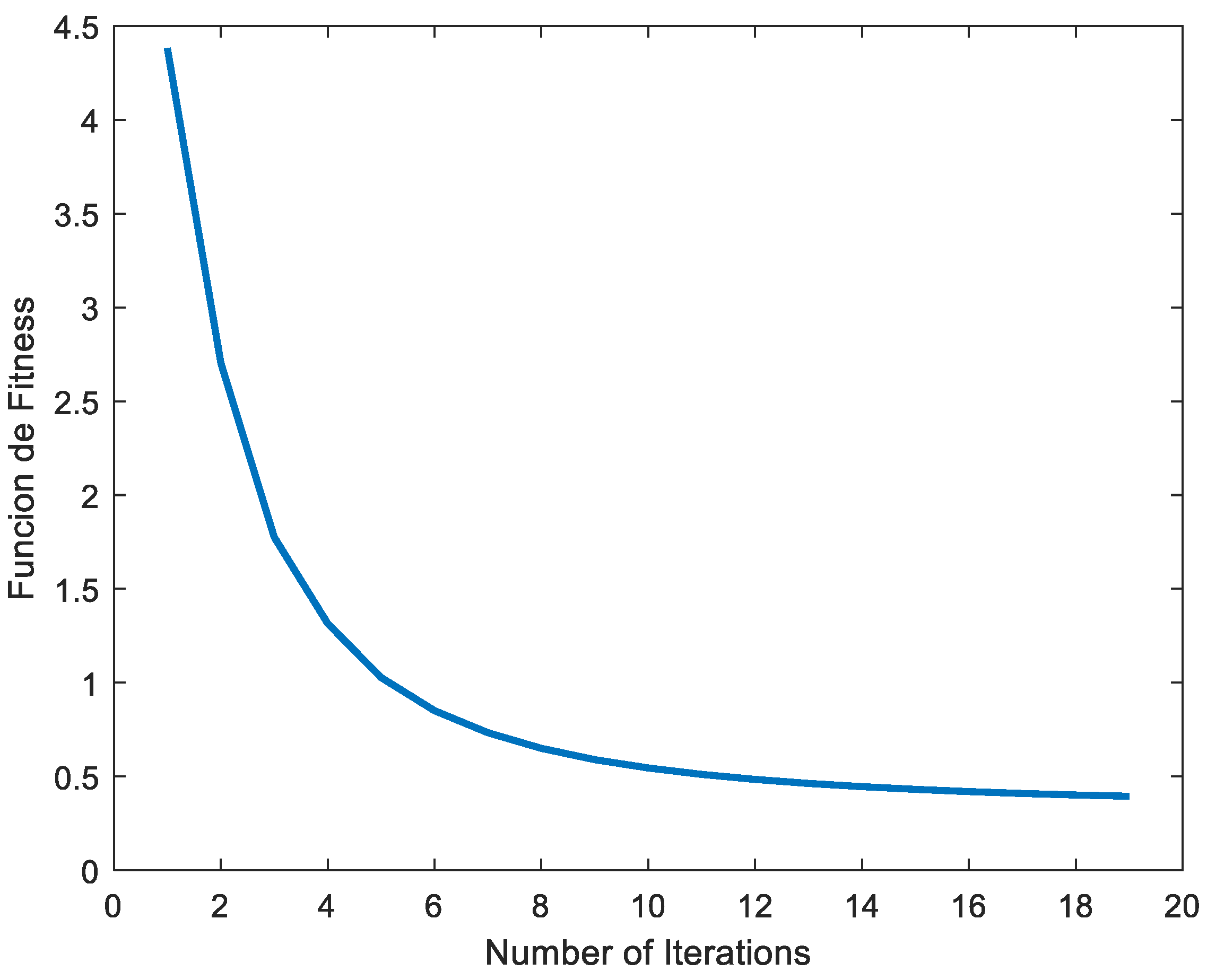
Figure 6.
Objective function evolution using PSO optimization algorithm for the MRAC fractional order case controller.
Figure 6.
Objective function evolution using PSO optimization algorithm for the MRAC fractional order case controller.
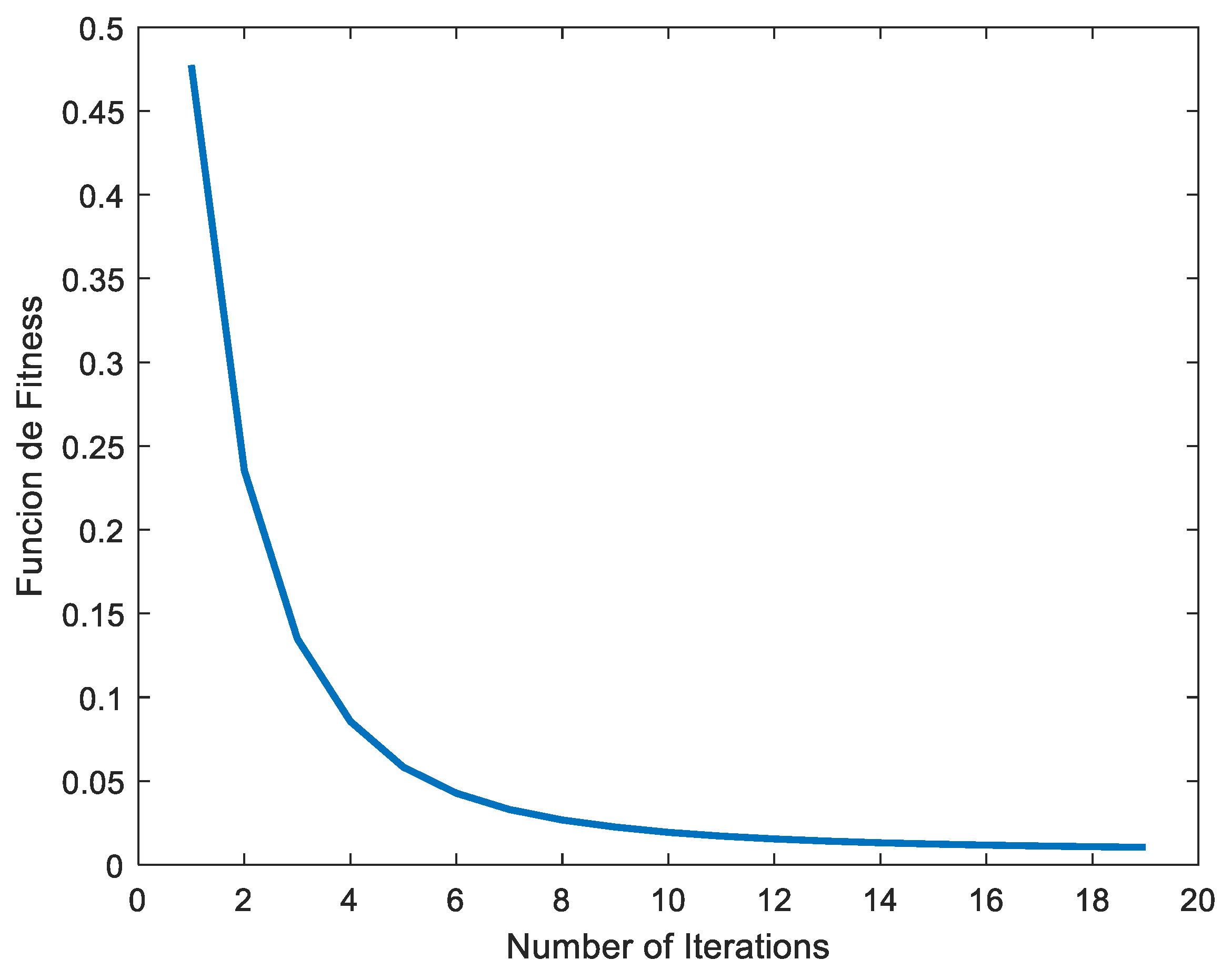
Figure 7.
Pitch rates response. IO-DMRAC (red color) and FO-DMRAC (green color). The reference signal is shown in blue color.
Figure 7.
Pitch rates response. IO-DMRAC (red color) and FO-DMRAC (green color). The reference signal is shown in blue color.
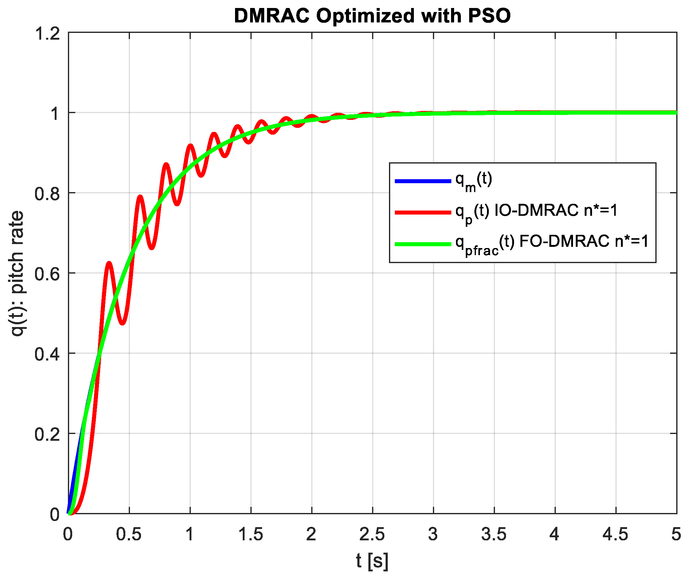
Figure 8.
Control effort using both type of controllers.
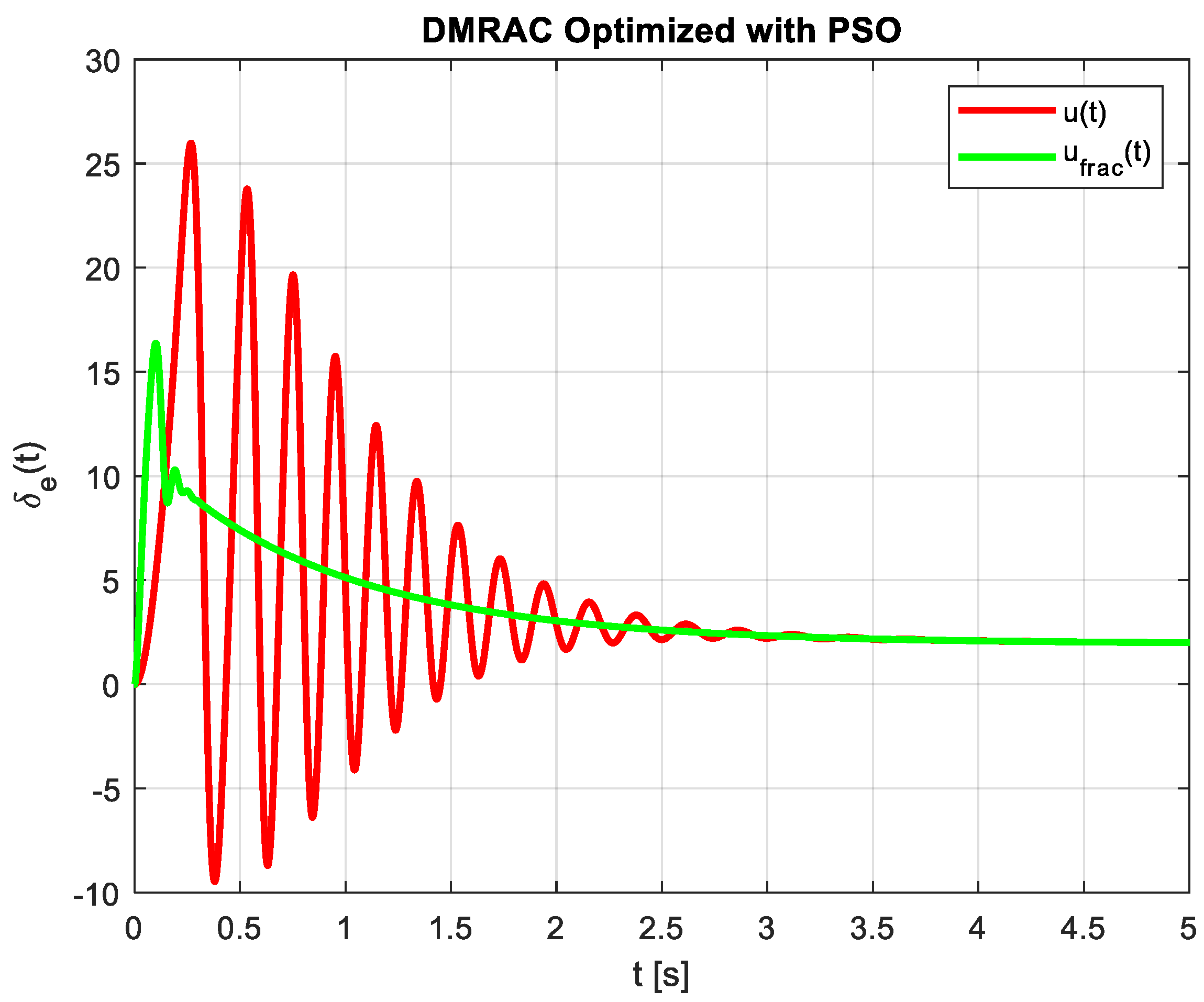
Figure 9.
Control output error using both type of controllers.
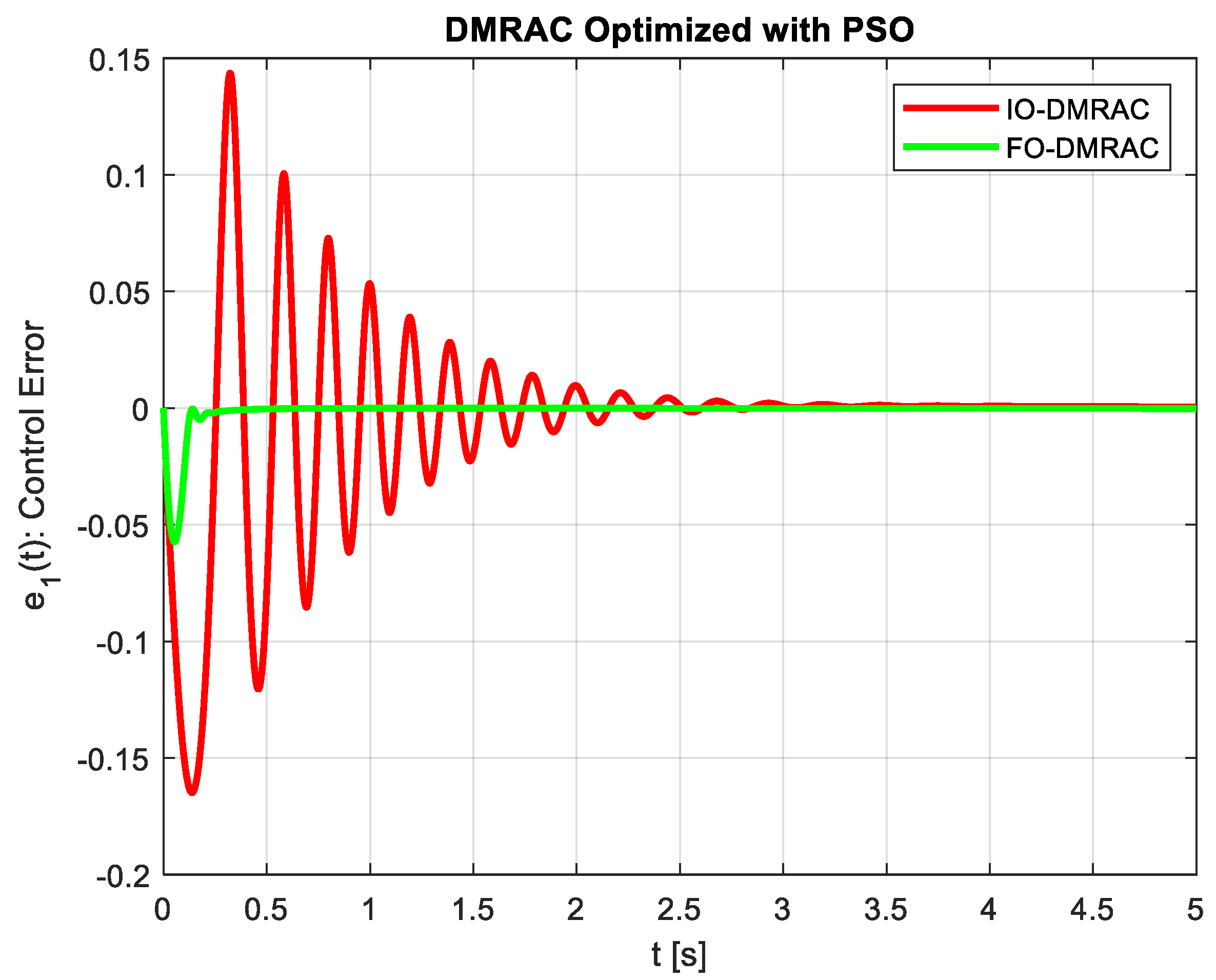
Figure 10.
Boundedness of the auxiliary signals .
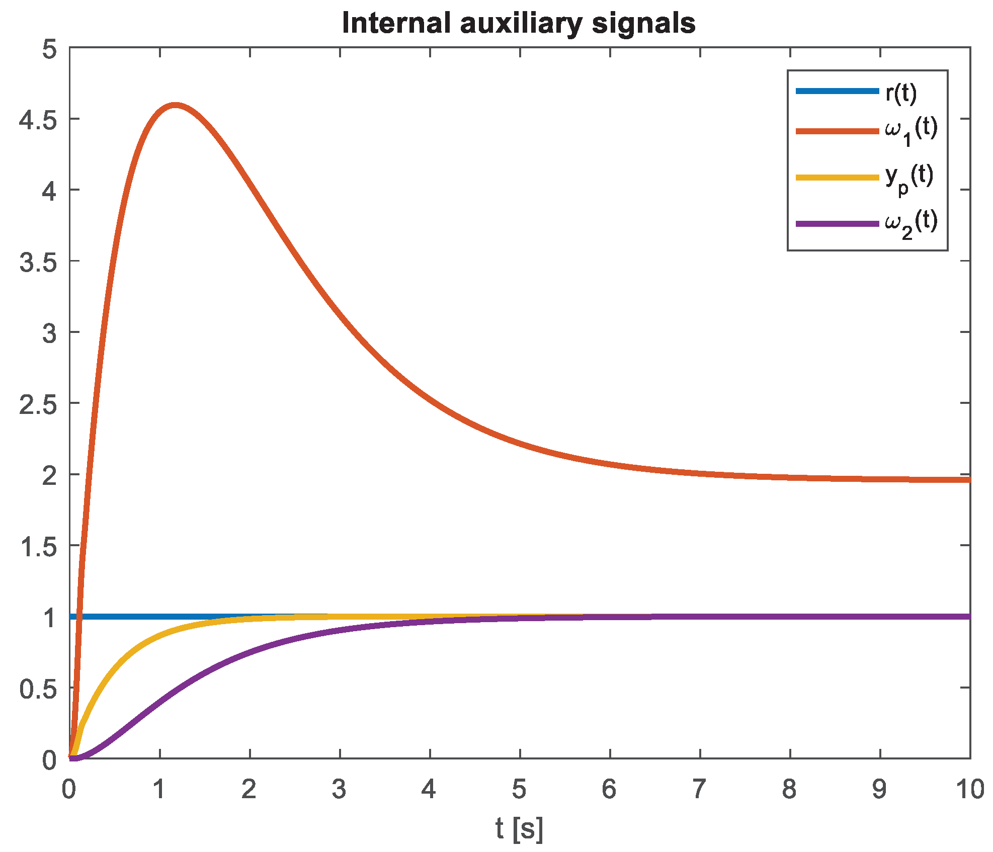

Table 1.
F-16 trim operating fligth conditions at sea level.
| Operating Conditions | |
|---|---|
| Altitude [feets] | 0 |
| Velocity [feet/sec] | 502 |
| Free-stream dynamic pressure= [lb/ft2] | 300 |
| Center of gravity in percent [%] | 0.35 |
Table 2.
FO-DMRAC and IO-DMRAC controller’s settings.
| Reference model | |
| Plant or Dynamic System to be controlled | |
| Control laws |
|
| Auxiliary signals |
1 |
| Control error | |
| Integer order adaptive law | |
| Fractional order adaptive law |
Table 3.
Objective function values using PSO algorithm.
| IO-DMRAC-PSO | 0.3946 |
| FO-DMRAC-PSO | 0,0104 |
Disclaimer/Publisher’s Note: The statements, opinions and data contained in all publications are solely those of the individual author(s) and contributor(s) and not of MDPI and/or the editor(s). MDPI and/or the editor(s) disclaim responsibility for any injury to people or property resulting from any ideas, methods, instructions or products referred to in the content. |
© 2024 by the authors. Licensee MDPI, Basel, Switzerland. This article is an open access article distributed under the terms and conditions of the Creative Commons Attribution (CC BY) license (https://creativecommons.org/licenses/by/4.0/).
Copyright: This open access article is published under a Creative Commons CC BY 4.0 license, which permit the free download, distribution, and reuse, provided that the author and preprint are cited in any reuse.


