Submitted:
24 June 2025
Posted:
26 June 2025
You are already at the latest version
Abstract
The design of the Aircraft Electrical Wiring Interconnection System (EWIS) is a core link to ensure the safe and reliable operation of aircraft. As one of the key technologies in EWIS design, the calculation of temperature rise characteristics of aircraft wire harnesses directly affects the safety margin of the system. However, existing calculation methods generally face the bottleneck of difficult balance between speed and accuracy, failing to meet the requirements of efficient and precise engineering applications. This paper conducts an in-depth study on this issue. Firstly, a high-fidelity finite element harness model is established to accurately obtain the convective heat transfer coefficients of wires and harnesses. Based on the analysis of influencing factors of the thermal network model for a single wire, an improved thermal resistance hierarchical wire thermal network model is proposed. A structure of "series thermal resistance within layers and iterative parallel between layers" is proposed to equivalently integrate and iteratively calculate the mutual thermal influence relationship between each layer of the harness, thereby constructing a hierarchical harness thermal network model. This model successfully achieves a significant improvement in calculation speed while effectively ensuring the accuracy of temperature rise results, providing an effective method for high-efficiency and high-precision EWIS design.
Keywords:
aircraft
; EWIS
; harness
; thermal temperature rise
; thermal network
1. Introduction
The temperature rise design capability of aircraft wire harnesses is a core indicator for measuring the design level of the Electrical Wiring Interconnection System (EWIS) of aircraft design units, and it is also a key technical support for the development of advanced aircraft with multi-electrification, integration, and high reliability [1]. In EWIS design, the accurate calculation of wire temperature rise directly determines the safety margin of the system—excessive temperature rise may lead to insulation aging, short circuits, or even fires. Therefore, calculation methods that balance engineering timeliness and physical accuracy are urgently needed.
Existing wire temperature rise calculation methods mainly include analytical methods and finite element simulation methods. Analytical calculation methods[2,3,4] quickly estimate the average/maximum temperature rise based on simplified formulas, with the fastest calculation speed. However, the derivation of formulas requires a large amount of data fitting and has disadvantages such as inability to reflect the axial temperature difference of wire harnesses, weak dynamic analysis capability, and high accuracy only within specific ranges, making it difficult to adapt to the temperature rise calculation of complex aircraft harnesses. The current-carrying capacity method [8,9,10,11] relies on IEC standard empirical formulas, but it has difficulties in convergence when harnesses are coupled, and formula verification is tedious. There are no special empirical formulas for aircraft harnesses. Traditional thermal network methods [12,13,14,15,16,17,18] have low dependence on empirical parameters and can analyze the temperature difference in the axial direction of wires, but they also have shortcomings such as calculation accuracy being related to the number of analysis nodes, inability to analyze complex harnesses, and unsuitability for analyzing dynamic temperature rise. Although simple to model and efficient in calculation, the solution accuracy highly depends on the accurate equivalence of thermal resistance topology. The finite element method [5,6,7] achieves high-precision simulation through 3D solid modeling, which can analyze the dynamic temperature rise of wire harnesses and perform relatively better in the axial temperature difference of harnesses than the thermal network method. However, for complex aircraft harnesses, model construction is time-consuming (hours-level) and consumes huge computing resources, unable to support batch harness analysis.
Aiming at the contradiction among speed, accuracy, and complexity, this paper proposes an iterative thermal network calculation model of "series within layers and parallel between layers". The main contributions of this paper are:
- Establishment of a high-precision thermal resistance hierarchical wire thermal network: The wire core conductor and insulation layer are divided into inner and outer layers. The model accuracy is corrected through the thermal resistance of the inner and outer layers. Meanwhile, a thermal resistance is added between the outer layer of the insulation and the external ambient air to simulate the heat dissipation loss due to changes in the material properties of the insulation and air, thereby correcting the model accuracy.
- Construction of a hierarchical harness thermal network model based on finite element model correction: Through the topology of the thermal resistance hierarchical wire thermal network, a structure of "series within layers and parallel between layers" is constructed. By conducting power-on simulations on the finite element single-layer model, the convective heat transfer coefficients of each layer’s thermal network model are corrected to complete the construction of the hierarchical harness thermal network model.
- Hierarchical thermal network iterative calculation method: Based on the hierarchical harness thermal network model, the interlayer influence is equivalently constructed through the finite element model results, and the rapid calculation of the hierarchical thermal network model is completed through the interlayer model iterative algorithm.
The structure of the full text is as follows: First, the establishment process of the high-fidelity finite element model is introduced, then the influencing factors of the wire thermal network model are analyzed and the thermal resistance hierarchical wire thermal network model is constructed. The wire thermal network model is expanded to obtain the hierarchical harness thermal network model, and finally, the fast calculation of the hierarchical harness thermal network model is realized through the iterative algorithm.
2. Construction of High-Fidelity Finite Element Model and Solution of Convective Heat Transfer Coefficient
The convective heat transfer coefficient h is affected by factors such as the geometric shape of the object, fluid properties (viscosity and density), flow state (laminar or turbulent flow), and flow mode (forced or natural convection), making it difficult to accurately calculate by analytical methods. The convective heat transfer coefficient can be obtained through the fluid simulation function of the finite element method, thereby simplifying a large number of complex calculations. The convective heat transfer coefficient can be calculated by the Nusselt number :
Both the air thermal conductivity and the Nusselt number affecting the convective heat transfer coefficient are difficult to obtain through direct calculation and need to be obtained with the help of simulation and experimental methods. Therefore, the flow field simulation function of finite element simulation software is used to directly obtain the convective heat transfer coefficient. The specific process is shown in Figure 1. The convective heat transfer coefficients of different gauge wires are solved through repeated cycles to obtain the relationship curve between the wire gauge and the convective heat transfer coefficient. Finally, the curve values of the convective heat transfer coefficient are substituted into the analytical formula.
When establishing the model by the finite element method, the following aspects need to be noted:
- Modeling and grid generation: Create the fluid domain and solid surface, and then use the meshing tool to discretize the geometric model to generate a computational grid suitable for calculating fluid flow and heat transfer. The meshing quality is crucial to the calculation results, directly affecting the calculation accuracy of wire temperature rise. Especially in the boundary layer area, sufficiently fine grids are required to capture the temperature gradient and velocity gradient of the fluid. The finite element grid is shown in Figure 2.
- Setting the boundary conditions of the model: Select a suitable laminar flow model or turbulent flow model according to the specific application scenario, and set the inlet boundary conditions and outlet boundary conditions, such as setting them as fixed pressure, flow rate, and ambient temperature. The grid diagram after setting the model boundary conditions is shown in Figure 3.
-
Setting the solver and calculating: Select an appropriate solver and numerical method, and set appropriate convergence criteria for iterative control. The convergence of the calculation process is judged by monitoring the changes in physical quantities (such as flow rate, temperature, residual, etc.). After the calculation is completed, check the temperature distribution, velocity field, and heat flux density of the flow field to ensure that the results meet the physical expectations.The air thermal conductivity under normal pressure is fixed, and the convective heat transfer coefficient should decrease with the increase of the wire diameter. The fluid model is used for simulation, then fitted, and then substituted into the wire thermal balance formula to reduce the calculation amount while ensuring the calculation accuracy. In the finite element model, only convective heat dissipation is set, and no radiation heat dissipation is set. The four surrounding boundaries are set as open boundaries, that is, allowing gas to flow in or out freely to simulate an infinite space. The simulation results of AWG10 wire under 101 A current at normal temperature and pressure are shown in Figure 4, where (a) is the temperature distribution and (b) is the flow velocity distribution.In order to obtain the convective heat transfer coefficients of different wires at different temperatures and altitudes, the relationship between temperature, pressure, and altitude is first established, as shown in Figure 5. To obtain the relationship between pressure and convective heat transfer coefficient, it is necessary to first use fluid finite element software to simulate the convective heat transfer coefficient under different pressures. The ambient pressures of 18 kPa, 40 kPa, 60 kPa, 80 kPa, and 101.4 kPa are selected to solve the convective heat transfer coefficients of single wires with different wire gauges, and the results are shown in Figure 6. At normal pressure of 101 kPa, the air convection heat dissipation effect is good, and the corresponding convective heat transfer coefficient is the largest. As the air pressure decreases, the convective heat transfer coefficient gradually decreases. The data are interpolated to obtain the variation relationship between the convective heat transfer coefficient and the wire diameter at any pressure, as shown in Figure 2, Figure 3, Figure 4, Figure 5, Figure 6 and Figure 6. According to Figure 7, the variation curves of the convective heat transfer coefficient with the wire diameter at the pressures of 75.35 kPa and 19.75 kPa are obtained, as shown in Figure 8.Under the premise that the arrangement of the harness is determined (the wire harnesses on the aircraft are basically arranged in a near-circular shape), a typical one is selected, and a finite element model is established to carry out the solution of the convective heat transfer system. Take a harness composed of 19 wires as an example, as shown in Figure 9.According to the constraints of the outer envelope size of the harness and the constraints of the wire model and quantity in the harness, the geometric model of the harness is established. When converting the geometric model to the finite element model, the wire conductor and insulation layer are solid heat transfer, which is easy to reach an equilibrium state, and their thermal power and heat transfer coefficient setting methods are the same as those of a single wire. For the air in the harness, due to the influence of the stacking and gaps of the harness, the flow velocity varies at different positions, so that the heat transfer coefficient also changes with the position. In order to simplify the model while ensuring the calculation accuracy, in the finite element model, the air is modeled in layers. According to the number of wire layers in the harness, the air is divided into the same number of layers from the center of the harness outer envelope to the outside, and an equivalent heat dissipation coefficient is set for each layer of air according to the calculation results of the fluid field.Then, the equivalent density and convective heat transfer coefficient of each layer of air in the harness are obtained through fluid field finite element simulation, and each wire is assigned values. After assigning the thermal power and convective heat transfer coefficient to each harness, the temperature matrix of the harness is analytically calculated by a numerical iteration method until each element value in the temperature matrix reaches the convergence condition.
3. Construction of Thermal Resistance Hierarchical Aircraft Wire Thermal Network Mode
Figure 10 shows the thermal network model of a traditional wire, which consists of loss input, core conductor thermal resistance, insulation layer thermal resistance, and the external environment. For calculation convenience, the thermal loss of the wire, and the thermal resistance of the conductor and insulation layer are all calculated in a unit length of 1 m. At the same time, temperature monitoring is set during model construction to record temperature rise calculation data. For a single wire, the traditional thermal network model idealizes the wire conductor as a solid conductor, so the thermal network model is relatively simple, but the calculation error is large.
Analyzing the differences between the thermal network and finite elements, the error sources of thermal network simulation may include:
- The distribution of the wire core and insulation layer is uneven. The material properties in the finite element will automatically change with temperature, but the thermal network model cannot consider this change, so the relative error is high. Considering that the wire loss is generated in a three-dimensional body, and the heat dissipation ultimately depends on the outer surface of the insulation layer, the larger the diameter, the worse the heat dissipation conditions of the wire, and the more uniform the temperature distribution in the wire. Therefore, the larger the diameter, the smaller the error in the thermal network.
- The thermal resistance change at the interface between the core and the insulation layer, and between the insulation layer and the air layer, as well as the change of materials, cause a certain loss of the wire’s heat dissipation effect. The wire is actually composed of individual cores, not a solid. There are also air gaps between the cores. The traditional thermal network model simplifies the wire conductor into a solid conductor. If each wire core is to be modeled, the thermal network model becomes very complex. Therefore, a new model simplification method needs to be created to ensure the accuracy of the calculation results and achieve model simplicity as much as possible. For this reason, this paper creates a thermal resistance hierarchical simplified thermal network method for the establishment and calculation of thermal network models.
Based on the simple model construction of a single wire, multiple cores are simplified into a solid conductor. If a refined wire model is to be established to construct a thermal network model, the thermal network model will be very complex. In order to ensure the calculation accuracy of the thermal network model without making the model too complex, this paper divides the wire core conductor and insulation layer into inner and outer layers. The model accuracy is corrected through the thermal resistance of the inner and outer layers. At the same time, a thermal resistance is added between the outer layer of the insulation and the external ambient air to simulate the heat dissipation loss due to changes in the material properties of the insulation and air, so as to correct the model accuracy, as shown in Figure 11.
In order to correct the above two factors, a thermal resistance hierarchical thermal network calculation model for a single wire as shown in Figure 12 is established.
Compared with the traditional thermal network model, the thermal resistance hierarchical thermal network model has made the following improvements and optimizations:
- In order to consider the temperature difference at different positions of the wire, the thermal resistance of the core and insulation layer is layered. The middle value of the corresponding diameter is used as the boundary, and the conductor and insulation layer are each divided into two layers. The inner layer temperature is relatively high, and the thermal resistance is specifically increased.
- A thermal resistance is added between the outer layer of the insulation and the external ambient air to simulate the heat dissipation loss due to changes in the material properties of the insulation and air. At the same time, to simulate the heat dissipation loss due to changes in the material properties of the conductor and insulation layer, the thermal resistance of the outer conductor and inner insulation layer is correspondingly increased.
- In order to ensure the uniformity of thermal resistance parameter verification and enable the same verification method to verify different types of wires, the parameters of the inner conductor, outer conductor, inner insulation, and outer insulation are analyzed. The thermal resistance of the inner conductor is increased by about 6.5 8.5% compared with the theoretical calculation value, and the thermal resistance of the outer conductor and inner insulation is increased by 3.5% 4.5% compared with the theoretical calculation.
Table 1 shows the comparison results of the finite element, thermal resistance hierarchical wire thermal network model, and experimental data for a single wire at 260 °C. It can be seen from Table 3-1 that the error of the thermal resistance hierarchical thermal network model is <6%. Although the error is still higher than that of finite element simulation, the simulation analysis accuracy has been greatly improved compared with the traditional single-wire thermal network model. Compared with finite element simulation, the calculation time is reduced from 10 20 s to about 5 s, which can be used for mass and rapid temperature rise calculation of wires.
4. Research on Aircraft Harness Thermal Network Model
4.1. Construction of Hierarchical Harness Thermal Network Model
Based on the thermal resistance hierarchical single-wire thermal network model in Section 3, the hierarchical harness thermal network model is constructed. Taking 7 wires as an example, Figure 13 shows the central wire and the first-layer architecture of the harness thermal network model. The thermal resistance hierarchical wire thermal network model of a single wire is packaged and combined. Each wire uses the thermal resistance hierarchical wire thermal network model, and the air thermal resistance between the wires within the layer is supplemented for the wires within the layer to form the first-layer harness thermal network model shown in Figure 14. The second, third, and fourth layers are established in sequence as shown in Figure 15.
4.2. Interlayer Iterative Fast Calculation Method
The idea of interlayer iteration is shown in Figure 16, and the detailed steps are as follows:
- Iterative calculation from outside to inside. Current is applied from outside to inside, and the temperature of the outermost layer is first simulated. The outside-to-inside iteration is reflected by overwriting the initial values of the ambient temperature parameters of the inner layer. Since the steady-state temperature is calculated, the temperature influence from the outer layer to the inner layer can be calculated by the average value of the temperatures of two to three adjacent wires. Then, for the next outer layer, the average temperature of the outer layer wires is set as its ambient temperature, and the corresponding current is applied for calculation to obtain the temperature value of the next outer layer in the first iteration from outside to inside. By analogy, until the central wire of the harness is reached, the temperature of the central wire of the harness can be obtained.
- Iterative calculation from inside to outside. From outside to inside is the average value, while the temperature influence of the central wire on the outer layer wires is the temperature rise transfer from a few wires to many wires, and the temperature drop is more obvious. By intercepting the results of multiple groups of finite element simulations, the influence coefficients are fitted into a function of the wire specification, interval distance, and convective heat dissipation coefficient as the correction coefficient for the temperature influence of each layer from inside to outside. Then, the iterative process from inside to outside is carried out. The influence is still reflected in the ambient temperature in the model on the thermal network, so as to realize the temperature simulation of the outer layer wires.
4.3. Comparison of Experimental Tests and Simulation Results
In this paper, the actual temperature rise characteristics of the wire harness are tested through experiments as reference values, and the thermal network calculation values are compared and analyzed with them. The schematic diagram of the wire harness experimental bench is shown in Figure 17, the experimental equipment is shown in Figure 18, and the experimental wire harness is shown in Figure 19. A power supply is loaded at one end of the wire, and a load is loaded at the other end. Three temperature sensors are installed on the surface of the wire harness insulation layer, and the test wires are connected to the test equipment. The test equipment transmits the test data to the display and recording equipment for analog display and recording of the test data. In the experiment, the current value applied to the wire is continuously increased from small to large, the temperature change on the wire surface is tested until the temperature rises and stabilizes at the maximum temperature that the wire can withstand, and the current value at this time is recorded. The current values when different specifications of wires reach the maximum temperature limit are repeatedly tested.
Table 2 shows the thermal network analysis results of a harness composed of 37 wires. Table 3 shows the analysis results of the harness thermal network model for a harness composed of 61 wires.
In terms of calculation time, the finite element method for calculating the harness temperature is affected by the mesh density of the single-wire model and the number of wires in the harness, with a calculation time of 10 20 minutes, while the thermal network method for calculating the harness model takes 1 2 minutes, with a speed increase of more than 60%.
5. Discussion
This study lays the groundwork for the accurate, rapid, and batch calculation of the thermal temperature rise in aircraft EWIS wiring harnesses. However, since the wiring harnesses investigated in this study were all in a straight physical configuration, while many EWIS wiring harnesses on aircraft feature bends, it may be necessary to consider the influence of the bend radius on the temperature rise in such cases. This aspect warrants further investigation in future research.
6. Conclusion
Aiming at the problem that the speed, accuracy, and model complexity of wire temperature rise calculation in aircraft EWIS design are difficult to coordinate, this paper proposes a harness thermal network modeling method based on thermal resistance hierarchy fusion iteration. The core contributions are as follows: By analyzing the mechanism of wire temperature rise, a thermal resistance hierarchical wire thermal network model is established, and based on this, it is extended to the harness level. Through hierarchical modeling and inner-outer layer iterative calculation methods, the calculation accuracy requirements of the harness thermal network model are met. The calculation errors of the wire harness are all within 8%, which meets the accuracy requirements and greatly reduces the model complexity and simulation time (80%). This method establishes a technical route of hierarchical decoupling modeling and dynamic fusion iteration based on high-fidelity finite element boundary input, providing an expandable engineering application scheme for the collaborative simulation of complex harness losses and temperature rise.
Author Contributions
Conceptualization, Tao Cao, Tianxu Zhao and Shumei Cui; methodology, Tao Cao and Shumei Cui; writing, Tao Cao; software, Tao Cao and Wei Li; validation, Tao Cao and Wei Li; investigation, Wei Li. All authors have read and agreed to the published version of the manuscript.
Funding
This research received no external funding.
Institutional Review Board Statement
Not applicable.
Informed Consent Statement
Not applicable.
Data Availability Statement
Not applicable.
Acknowledgments
Thanks for the help from Shumei Cui and Wei Li.
Conflicts of Interest
The authors declare no conflicts of interest.
Abbreviations
The following abbreviations are used in this manuscript:
| EWIS | Electrical Wiring Interconnection System |
References
- Hu, X. Research on Electrical Wiring Design and Verification of Civil Aircraft. In Proceedings of the 2022 2nd International Conference on Electrical Engineering and Control Science (IC2ECS); IEEE, 2022; pp. 96–100. [Google Scholar]
- Cecchi, V.; Miu, K.; Leger, A. S.; et al. Study of the impacts of ambient temperature variations along a transmission line using temperature-dependent line models. In Proceedings of the 2011 IEEE Power and Energy Society General Meeting; IEEE, 2011; pp. 1–7. [Google Scholar]
- Cecchi, V.; Leger, A. S.; Miu, K.; et al. Incorporating temperature variations into transmission-line models. IEEE Transactions on Power Delivery 2011, 26, 2189–2196. [Google Scholar] [CrossRef]
- Nigol, O.; Barrett, J. S. Characteristics of ACSR conductors at high temperatures and stresses. IEEE Transactions on Power Apparatus and Systems 1981, (2), 485–493. [Google Scholar] [CrossRef]
- Zhou, X.; Wen, D.; Wang, S.; Liu, Y.; Jiang, Y.; Li, T. Simulation Analysis of Bundle Conductors Thermal Field in High Voltage Overhead Transmission Lines. Electrotechnics Electric 2017, (03), 20–22. [Google Scholar]
- Yu, X.; Yao, L.; Zhao, S.; Yu, S.; He, A. Infrared On-line Diagnosis Method for Recessive Defect of Aviation Wire Insulation Layer. Ship Electronic Engineering 2019, 39, 199–203. [Google Scholar]
- Al-Dulaimi, A. A.; Guneser, M. T.; Hameed, A. A.; et al. Adaptive FEM-BPNN model for predicting underground cable temperature considering varied soil composition. Engineering Science and Technology, an International Journal 2024, 51, 101658. [Google Scholar] [CrossRef]
- Sellers, S. M.; Black, W. Z. Refinements to the Neher-McGrath model for calculating the ampacity of underground cables. IEEE Transactions on Power Delivery 1996, 11, 12–30. [Google Scholar] [CrossRef]
- Anders, G. J.; Coates, M. Mohamed ampacity calculations for cables in shallow troughs. IEEE Transactions on Power Delivery 2010, 25, 2064–2072. [Google Scholar] [CrossRef]
- IEC 60287-1-1:1994 Calculation of the current rating of electric cables, part1: current rating equations (100% load factor) and calculation of losses, section 1: general; International Electrotechnical Commission: 1994.
- IEC 60287-2-1 AMD 1-2006 Electric cables-calculation of the current rating-part 2-1: thermal resistance; calculation of thermal resistance; amendment 2; International Electrotechnical Commission: 2006.
- Henke, A.; Frei, S. Transient temperature calculation in a single cable using an analytic approach. Journal of Fluid Flow, Heat and Mass Transfer (JFFHMT) 2020, 7, 58–65. [Google Scholar] [CrossRef]
- Henke, A.; Frei, S. Analytical Approaches for Fast Computing of the Thermal Load of Vehicle Cables of Arbitrary Length for the Application in Intelligent Fuses. In Proceedings of the VEHITS; 2021; pp. 396–404. [Google Scholar]
- Benthem, R.; Grave, W.; Doctor, F.; et al. Thermal analysis of wiring bundles for weight reduction and improved safety. In Proceedings of the 41st International Conference on Environmental Systems; 2011; p. 5111. [Google Scholar]
- Ming, L.; Gang, L.; Yu-ting, L.; et al. Study on thermal model of dynamic temperature calculation of single-core cable based on Laplace calculation method. In Proceedings of the 2010 IEEE International Symposium on Electrical Insulation; IEEE, 2010; pp. 1–7. [Google Scholar]
- Chenzhao, F.; Wenrong, S.; Lingyu, Z.; et al. Research on the fast calculation model for transient temperature rise of direct buried cable groups. In Proceedings of the 2018 12th International Conference on the Properties and Applications of Dielectric Materials (ICPADM); IEEE, 2018; pp. 646–652. [Google Scholar]
- Xiao, R.; Liang, Y.; Fu, C.; et al. Rapid calculation model for transient temperature rise of complex direct buried cable cores. Energy Reports 2023, 9, 306–313. [Google Scholar] [CrossRef]
- Liang, Y.; Cheng, X.; Zhao, Y. Research on the rapid calculation method of temperature rise of cable core of duct cable under emergency load. Energy Reports 2023, 9, 737–744. [Google Scholar] [CrossRef]
Figure 1.
Building process of finite element model
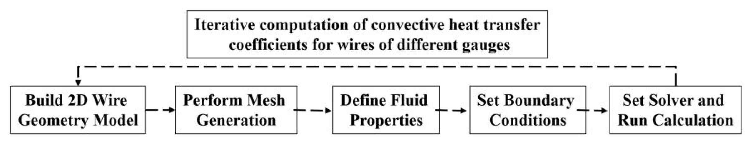
Figure 2.
Finite element grid diagram
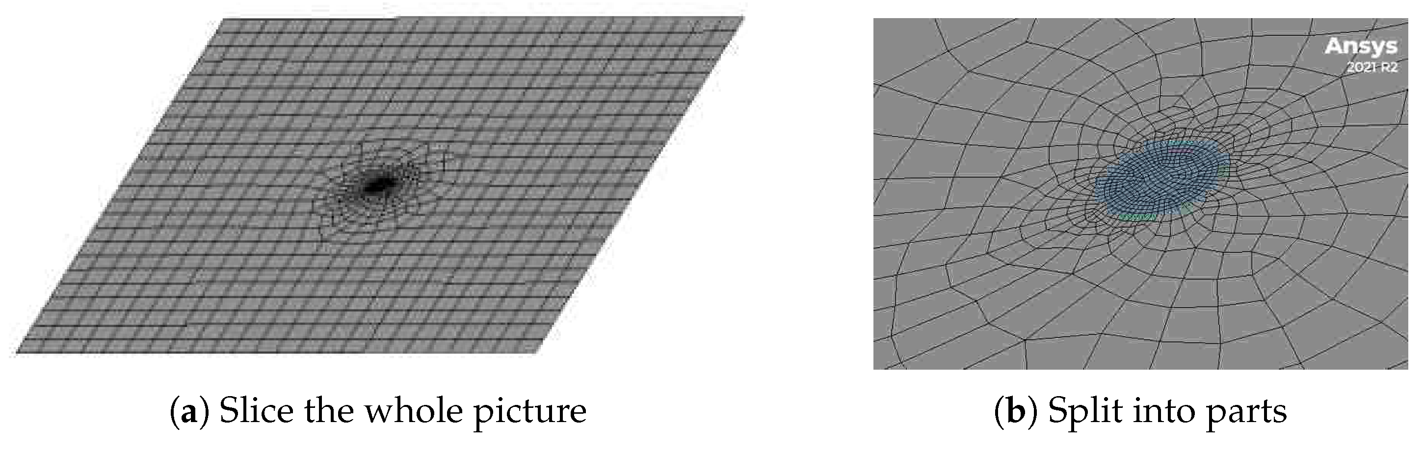
Figure 3.
Boundary setting grid diagram
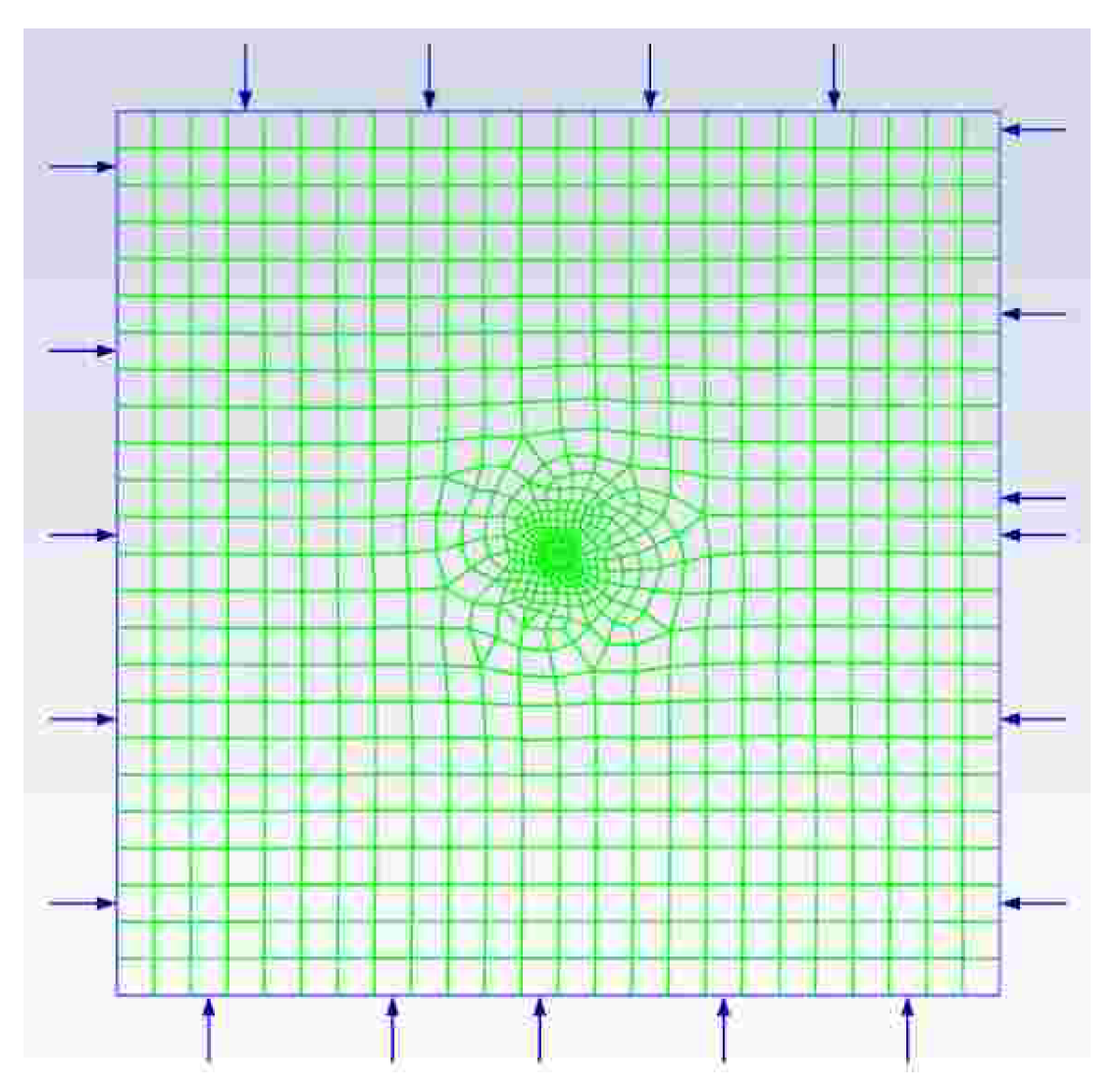
Figure 4.
Fluid simulation cloud map
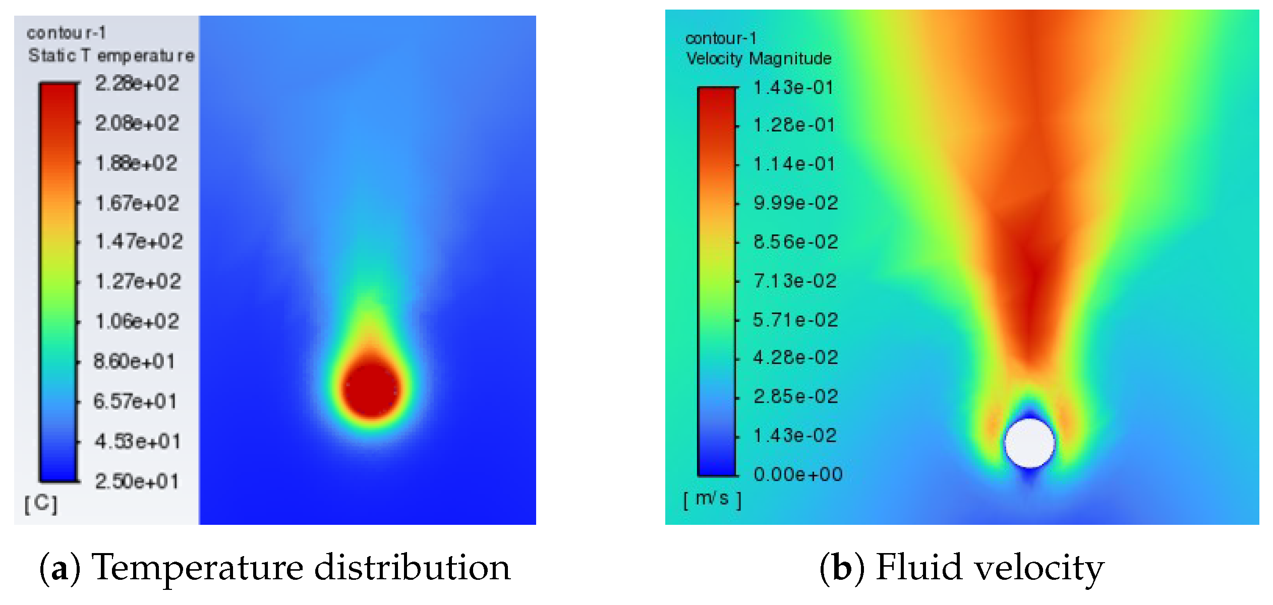
Figure 5.
Fluid simulation cloud map
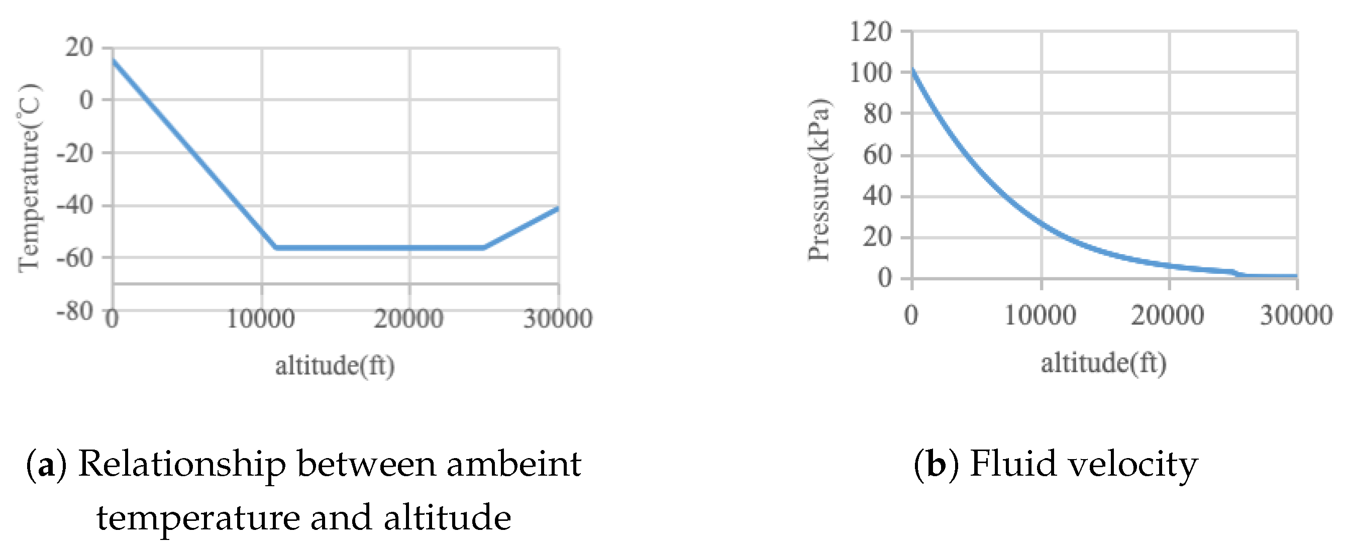
Figure 6.
Heat transfer rate of different wire diameter and pressure
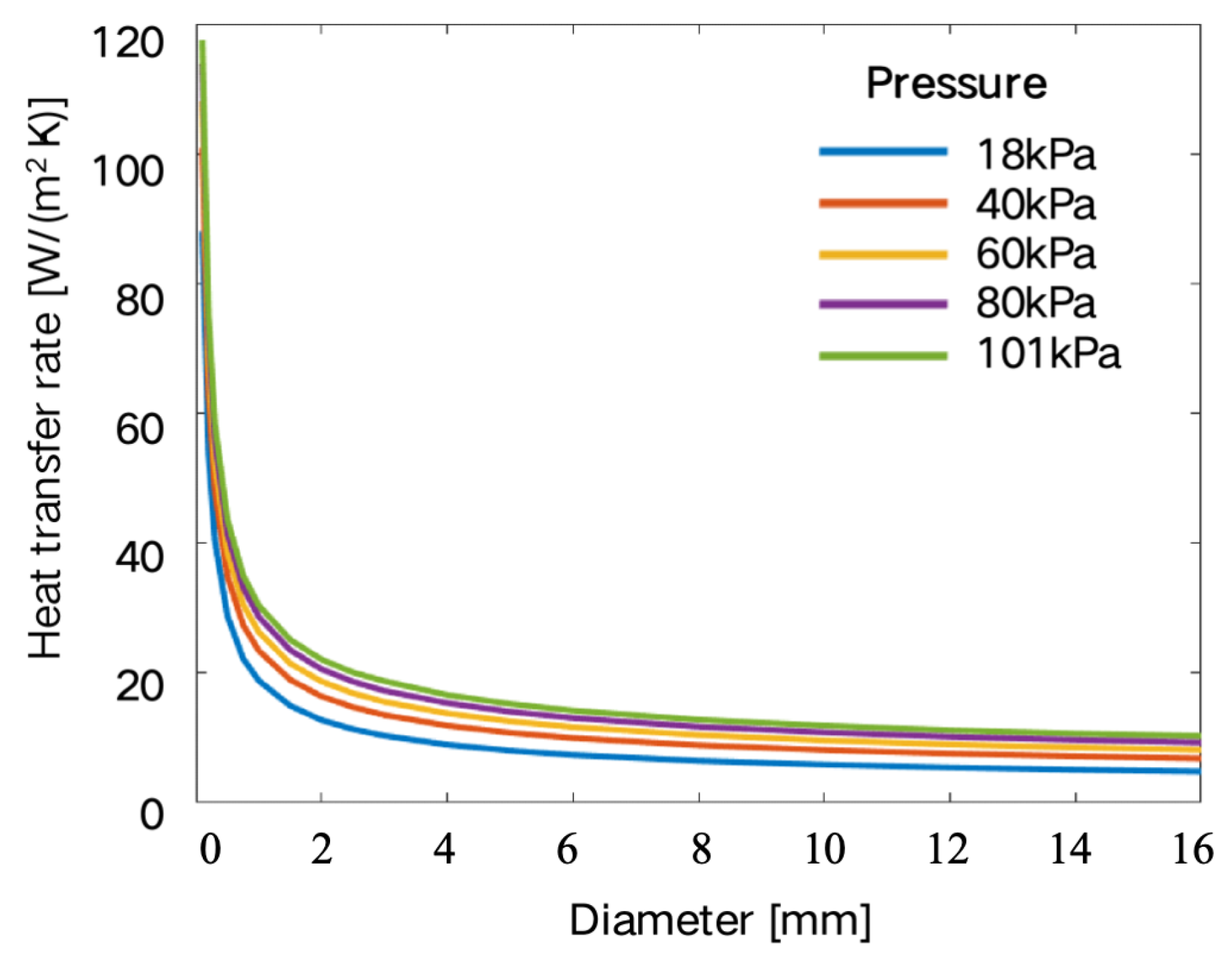
Figure 7.
Heat transfer rate of different wire diameter and pressure
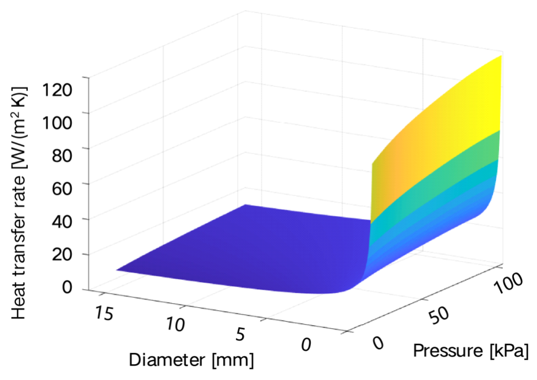
Figure 8.
Heat transfer rate of different wire diameter and pressure after interpolation
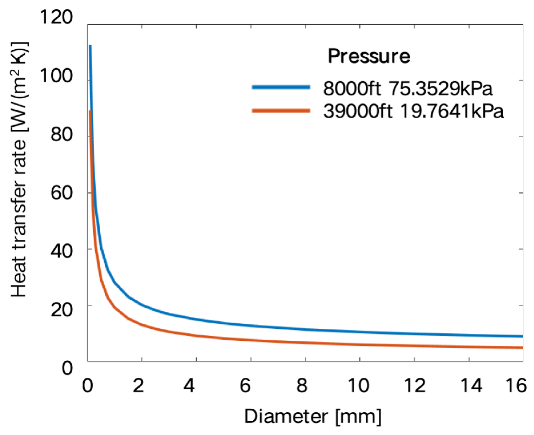
Figure 9.
Variation of heat transfer rate with wire diameter under 75.35 kPa, 19.75 kPa
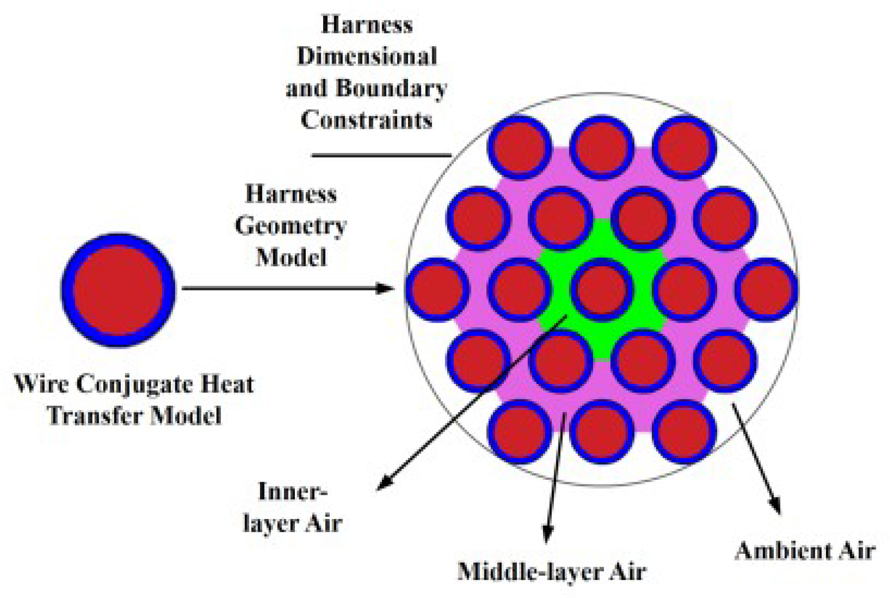
Figure 10.
Thermal network model of a traditional wire
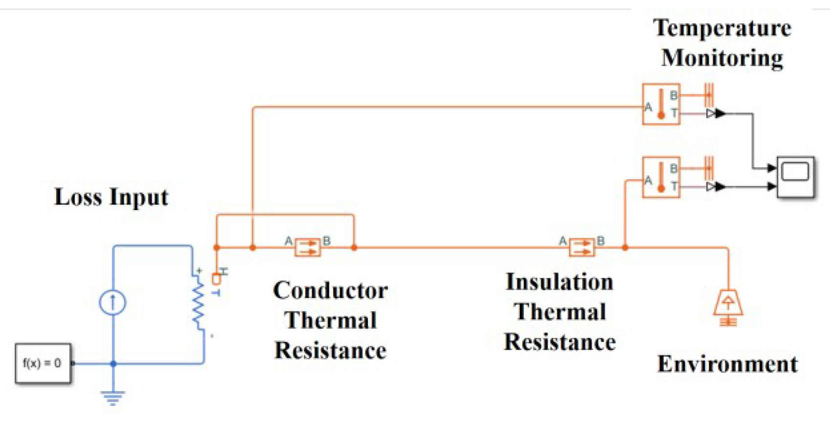
Figure 11.
Thermal network model correction ideas
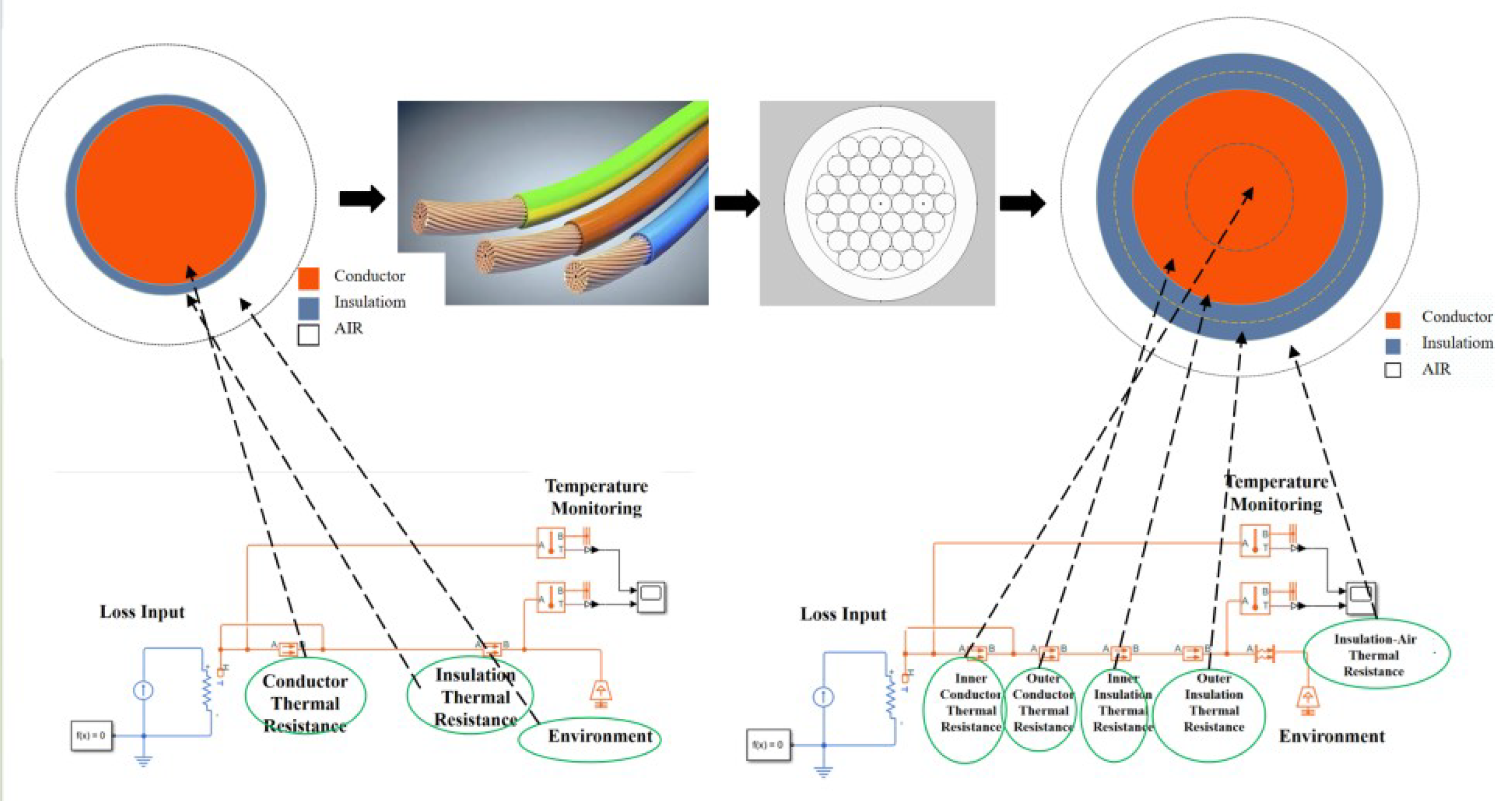
Figure 12.
Modified single-wire thermal network model
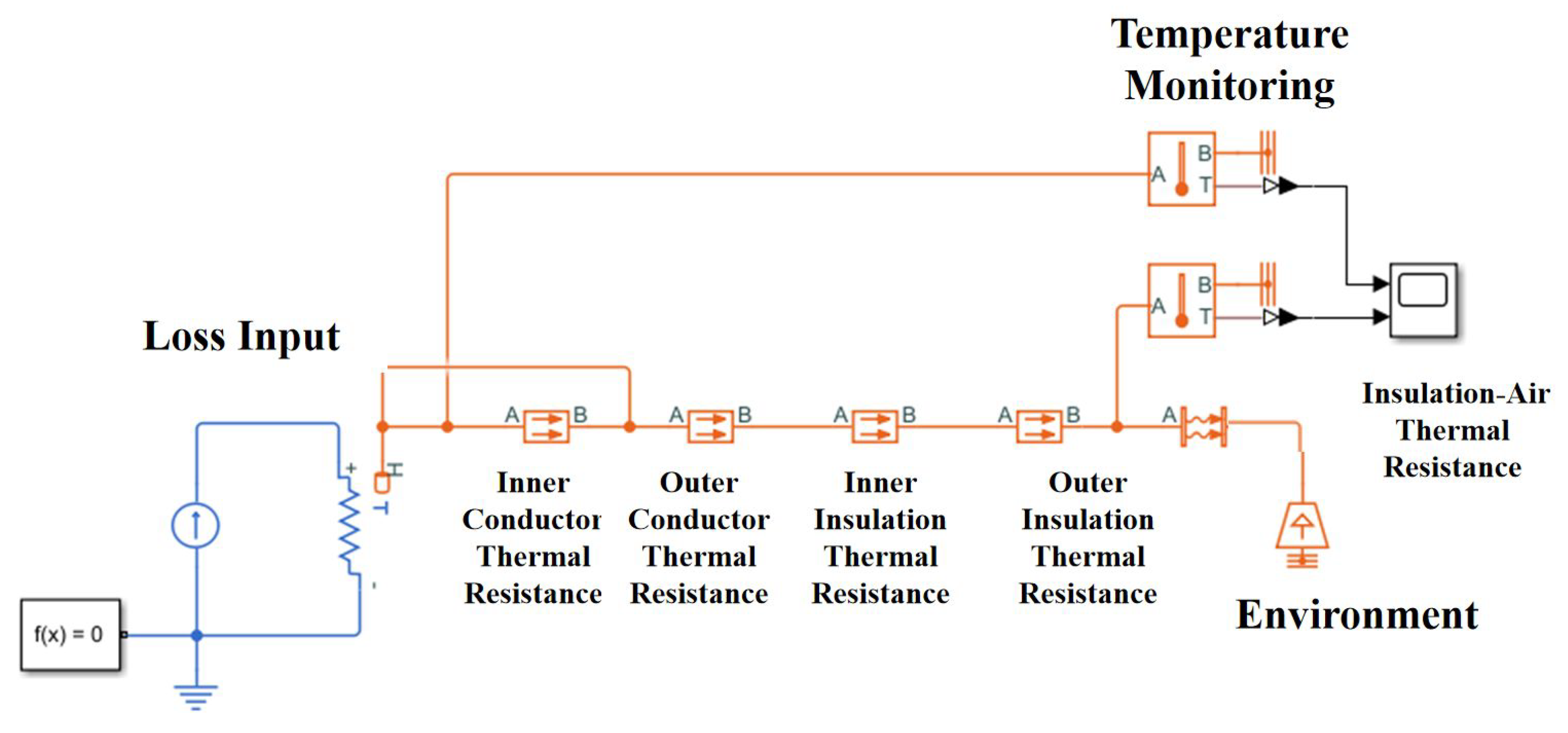
Figure 13.
Calculation method of hierarchical thermal network model (taking seven wire harnesses as an example)
Figure 13.
Calculation method of hierarchical thermal network model (taking seven wire harnesses as an example)
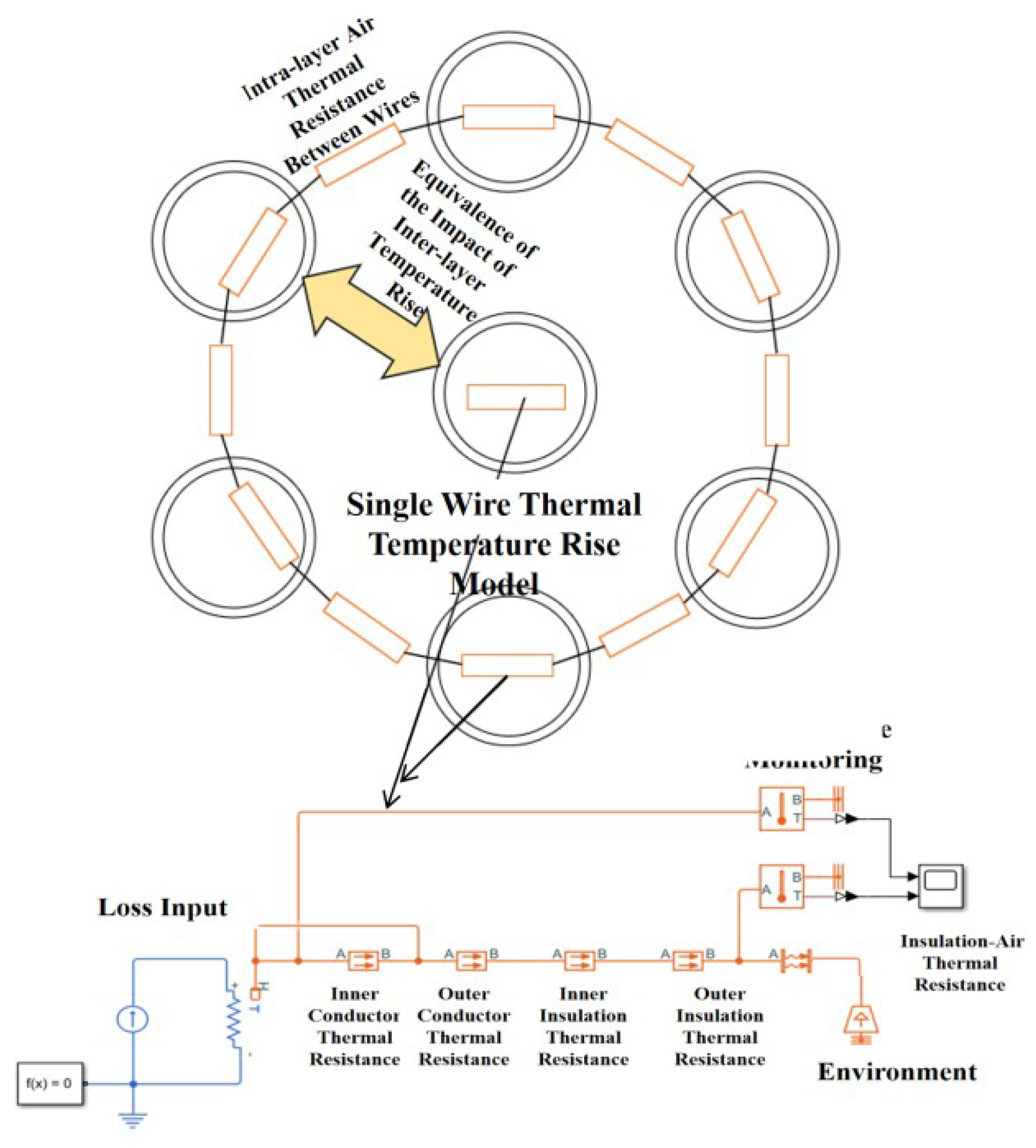
Figure 14.
First layer wiring harness thermal network model
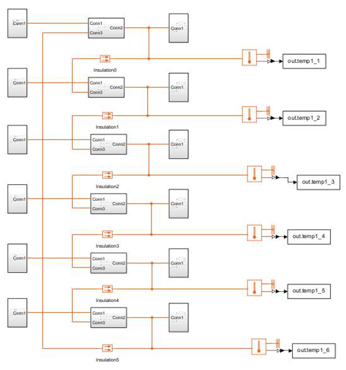
Figure 15.
Schematic diagram of the hierarchical model of the harness thermal network

Figure 16.
The process of building a harness thermal network model
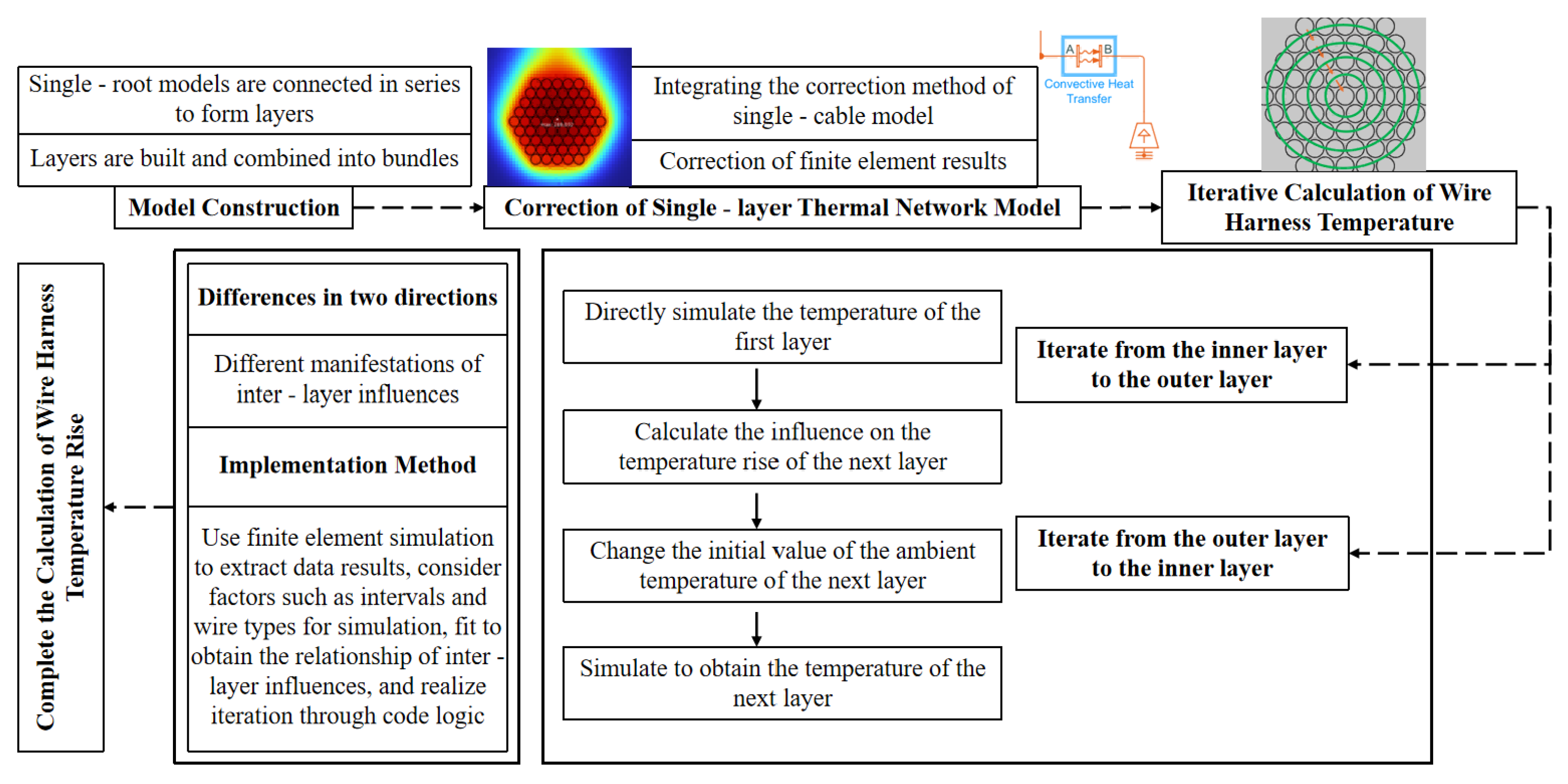
Figure 17.
Schematic diagram of the experimental bench
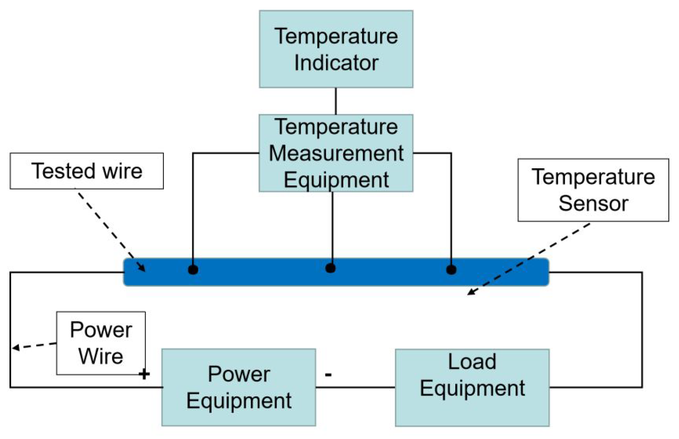
Figure 18.
Experimental equipment
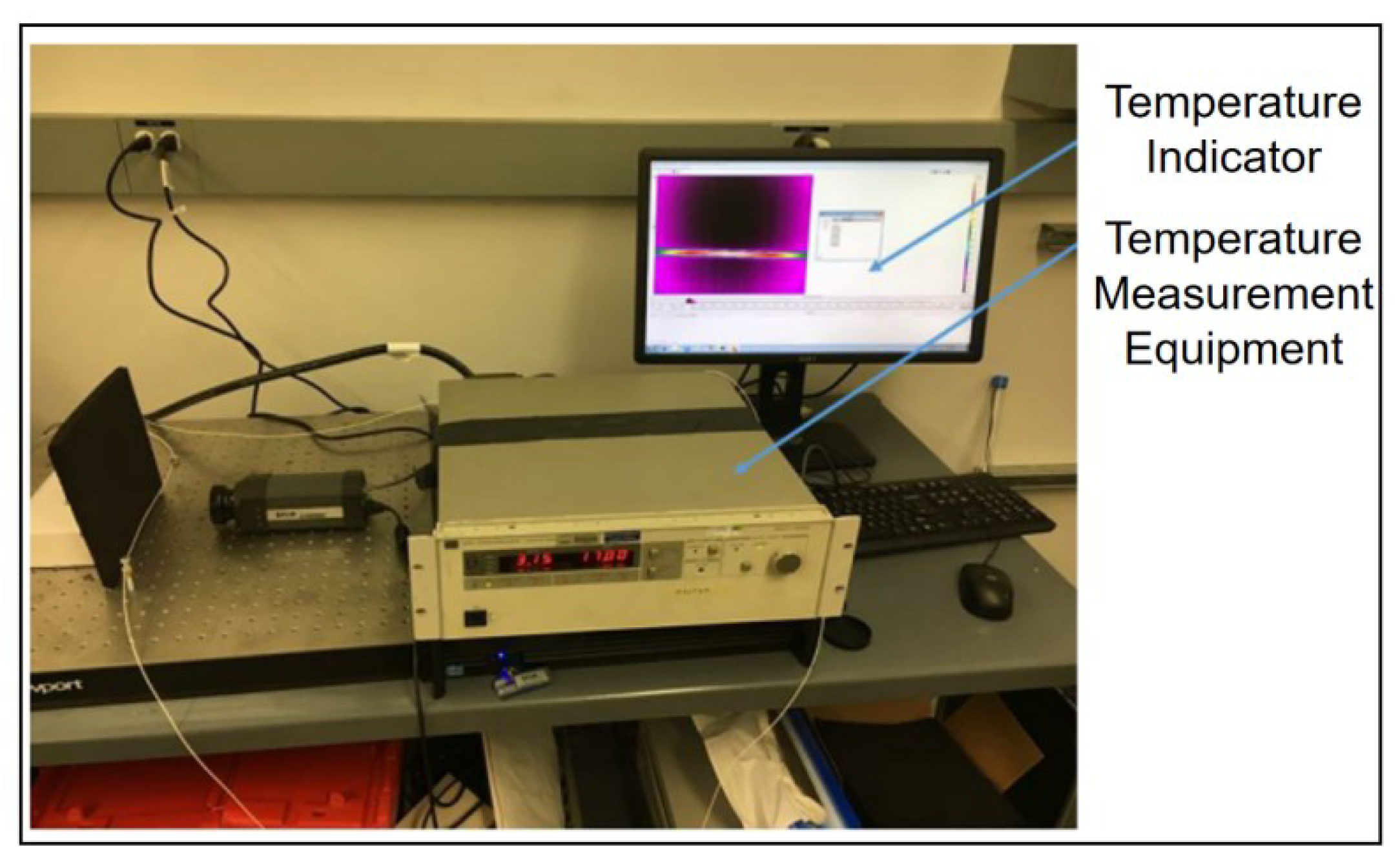
Figure 19.
Test experiment photo
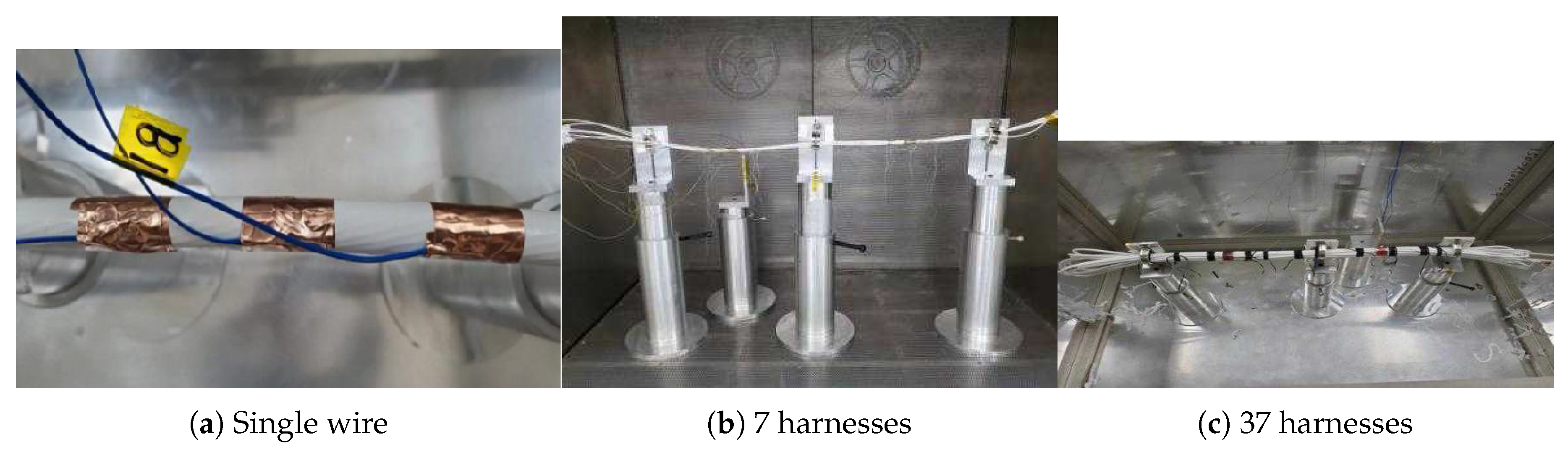

Table 1.
Comparison and analysis of 260℃ simulation calculations and experimental data for different wires.
Table 1.
Comparison and analysis of 260℃ simulation calculations and experimental data for different wires.
| Wire Gauge | 260℃ Experimental Test Current (A) | FEM Simulation Current (A) | Thermal Network Model Simulation Current (A) | FEM Model Error (%) | Thermal Network Model Error(%) |
|---|---|---|---|---|---|
| AWG4 | 284.2 | 288.4 | 269.7 | 1.478 | 5.10 |
| AWG12 | 78.9 | 80.9 | 74.5 | 2.535 | 5.58 |
| AWG12 | 30.0 | 31.8 | 28.3 | 6.000 | 5.67 |
Table 2.
37 AWG16 wires make up the harness analysis results
| Power-on Condition | Tested(℃) | FEM(℃) | Thermal Network Model Simulation Current (A) | FEM Model Error (%) | Thermal Network Model Error(%) |
|---|---|---|---|---|---|
| Central 43.66A | |||||
| Peripheral 0A | 171.01 | 178.6 | 180.4 | 4.4 | 5.5 |
| Central 43.66A | |||||
| Peripheral 9.1A | 260.89 | 268.7 | 271.6 | 3.0 | 4.1 |
| All 10.5A | 152.86 | 158.5 | 159.4 | 3.7 | 4.2 |
| All 12.3A | 200.2 | 208.2 | 210.6 | 4.0 | 5.1 |
| All 14.1A | 257.26 | 268.1 | 269.0 | 4.2 | 4.5 |
Table 3.
61 AWG18 wires make up the harness analysis results
| Power-on Condition | Tested(℃) | FEM(℃) | Thermal Network Model Simulation Current (A) | FEM Model Error (%) | Thermal Network Model Error(%) |
|---|---|---|---|---|---|
| Central 38.93A | |||||
| Peripheral 0A | 173.82 | 180.5 | 185.2 | 3.843 | 6.56 |
| Central 38.93A | |||||
| Peripheral 6.2A | 263.08 | 271.6 | 284.7 | 3.239 | 8.21 |
| All 7.4A | 150.5 | 155.1 | 161.5 | 3.056 | 7.31 |
| All 8.7A | 200.7 | 207.9 | 213.5 | 3.587 | 6.38 |
| All 10.05A | 261.72 | 269.4 | 281.3 | 2.934 | 7.49 |
Disclaimer/Publisher’s Note: The statements, opinions and data contained in all publications are solely those of the individual author(s) and contributor(s) and not of MDPI and/or the editor(s). MDPI and/or the editor(s) disclaim responsibility for any injury to people or property resulting from any ideas, methods, instructions or products referred to in the content. |
© 2025 by the authors. Licensee MDPI, Basel, Switzerland. This article is an open access article distributed under the terms and conditions of the Creative Commons Attribution (CC BY) license (http://creativecommons.org/licenses/by/4.0/).
Copyright: This open access article is published under a Creative Commons CC BY 4.0 license, which permit the free download, distribution, and reuse, provided that the author and preprint are cited in any reuse.


