
Submitted:
23 June 2025
Posted:
25 June 2025
You are already at the latest version
Abstract
A theoretical prediction of the strong coupling constant αs (μ) based on a non-perturbative framework derived from Bridge Theory (BT) is presented, in which strong interactions emerge from electromagnetic dipole interactions (DEMS) between fractional charges. Without relying on Quantum Chromodynamics (QCD) or renormalization group formalism, we derive a functional expression for αs as a function of energy scale μ , based on the spatial and energetic configuration of quark interactions. The resulting function exhibits asymptotic freedom at high energies and yields values of αs in close agreement with experimental data in the 91–4000 GeV range. The predicted behaviour matches the experimental running of αs across various particle production channels, including e-e+ , p-p+ , and heavy boson processes. The model provides a geometric interpretation of strong coupling as an emergent electromagnetic effect governed by the local structure of the dipole system, avoiding the need for additional gauge fields. These results suggest that the strong coupling constant may derive from universal interaction principles and that strong force dynamics could be reinterpreted within an electromagnetic framework. The method is fully predictive and does not rely on fitted parameters.
Keywords:
bridge theory
; hadrons
; standard model
; strong interaction
1. Introduction
This paper proposes a very particular approach to the problem of variability with the energy scale of the coupling constant of the strong interaction . The approach, developed in the framework of Bridge Electromagnetic Theory (or in short Bridge Theory), has deep roots in Maxwellian electromagnetism [1] and suggests a clear framework of unification between electromagnetic and strong forces, introducing a possible general solution to the problem of the running coupling. The developed model allows to obtain a unified view of electromagnetic and strong interactions, paving the way for a unique theory based on the Bridge Theory (BT).
BT is a relativistic quantum theory of electromagnetic interactions between particles. Developed entirely on the basis of Maxwellian electromagnetism, BT has the advantage over many other theories of being completely self-consistent. In fact, the theory makes use of Maxwell's electromagnetism to explain typically quantum and relativistic phenomenologies, demonstrating that these two apparently incompatible aspects of the physical world have the same origin [2,3]. In this sense, it can be said that BT is a conceptual, phenomenological and formal bridge between different theories, able of justifying their synergistic use within the same phenomenological context.
The basic idea arose from the consideration that an electromagnetic interaction between two charged particles generally creates an electromagnetic dipole considered in the context of electromagnetism as point-like, therefore with a symmetrical electromagnetic field emitting a spherical wave.
If we make a leap in scale, their interaction at the nano level takes place with a non-zero collision parameter, therefore with a finite dipole moment that has an evolution over time. This implies that the dipole electromagnetic field has a cylindrical symmetry, so it has a Poynting vector that is not always radial with respect to the virtual centre of the dipole and due to the process of approaching and moving away of the two interacting particles, it lives only for a finite time determined by the collision parameters. Because of cylindrical symmetry, not all of the energy produced in the interaction can be emitted instantaneously, which is the case with spherical symmetry. A part of the energy and momentum associated with the transverse component of the Poynting vector is localized in the source zone and represents, quantitatively and formally, the quantum of energy exchanged in the interaction between the two particles. The effective duration of the interaction is where is the minimum distance reached by the two particles during the dipole formation, identical to the emission wavelength. This idea, proposed under form of conjecture [4] in 1989, was proved in 1990 with the explanation of the nature of the Sommerfeld and Planck constants [5,6], represents the starting point for the BT.
Compared to all other quantum theories in which quantization must be introduced as a fundamental principle, BT has the advantage of being self-quantized, i.e. given the particular way of interaction between charges and electric fields, it is possible to determine autonomously and without introducing extraneous constants, the electromagnetic coupling constant and from this to coherently obtain the value of the Planck action constant. The values obtained are in excellent agreement with those obtained experimentally but unlike what happens for standard theories these are not true constants, because they are subject to changes according to the constraints and external forces to which the interacting system is subjected, as in the case of the electron-proton capture process that gives rise to a hydrogen atom [7].
Formally, BT agrees with both formalism and the standard phenomenologies of relativity and quantum mechanics, only some basic phenomenologies disagree as they are consistent with the fundamental distinguishing elements of BT and that is why they can provide valuable experimental support to test the theory. In fact, in this framework, the interactions between charged particles follow a different phenomenology than usual which nevertheless leads to a result consistent with the experimental one.
In BT, an unusual way of conceiving interactions between charged particles has therefore been developed. In fact, interactions in a group of particles occur as superpositions of dipoles and not as multipolar interactions. Each dipole is formed by a possible combination of two of the particles, each of which forms a Dipole Electromagnetic Source (DEMS). The electromagnetic structure of each DEMS, if formed by pairs of particles, corresponds formally and quantitatively to a quantum of energy, therefore to an exchange photon that mediates the interaction between the two particles, otherwise, although having the same formal appearance of a quantum, the value of its constant of action can be very different from that of Planck's constant.
For example, for a pair of particles with one unit of electric charge, such as the interacting electron and proton, the action constant coincides with the value of Planck's constant but may be slightly different in the case of unconstrained free interaction and in the case of bound interaction as in a hydrogenoid atoms [8]. This result allows us to obtain an explanation consistent with Maxwellian electromagnetism of the reason for the value of the electromagnetic coupling constant of Sommerfeld which can take slightly different values depending on the type of experimental measurement system used.
The aim of this article is to demonstrate that the same phenomenology and the same principles applied to the electromagnetic interactions between integer electric charges, when applied to hadrons, provide results in excellent agreement with the experimental measurements of the strong coupling constants, providing a prediction of the coupling value as a function of the coupling energy, therefore as a function of the scale value, demonstrating that the strong interaction is not another force, but is a different way of manifesting itself from the electromagnetic force and that it is therefore unifiable in a single theoretical scheme.
To achieve our goal, we will first deal with the interaction between two particles with any electric charge. One will then apply the model to the direct electromagnetic interaction of a pair of electrons by obtaining the structure function and calculating its action, and then extend the model to single pairs of quarks and a pair of protons. One will calculate theoretically the low-energy, high-energy strong coupling constant assuming the production of up to three bosons, then develop a method for the generalized calculation of the coupling constant at any energy level.
2. Electromagnetic Interaction of Two Charged Particles Mediated by DEMS
Following the principles of BT in Ref. [2], to generalize the formation model of a DEMS produced by the direct electromagnetic interaction of two charged particles, regardless of their actual charge value: and , where and are dimensionless charges associated with a DEMS with an action value expressed in the Dirac form , the DEMS produced localize an energy exchange
with wavelength equal to the minimum distance achieved by the two particles during their approach.
The value of the action written in Gaussian units
depends on the value of the electromagnetic structure function of the DEMS
where the function in the integral at first term at R.s. of the Eq. (3)
is directly related to the structure of the electromagnetic field associated to the transversal component of the Poynting vector of the DEMS produced during the interaction, and the second term at R.s. of the Eq. (3), is related to the Coulombian term due to the electrostatic work of the two interacting particles. Therefore, considering the Eq. (3) and (4), the theoretical value of the structure function for an interaction between two charged particles, depends on the value of the dipole ratio and by the value of the dimensionless charges that parametrize it.
The structure constant (3), describes the ability of the electromagnetic field of the DEMS to localize energy as a function of the dipole ratio and of the dimensionless charges value of the interacting particles. It easy to verify that only for pairs of particles Eq. (3) can be simplified in the form
therefore, using Eq. (3) the electromagnetic coupling constant of two particles is and for pairs of charges using Eq. (5) becomes , where α represents the intensity of the interaction between two particles with unit of charge, i.e., .
To exam the behaviour of the coupling constant α as a function of the dipole ratio, using Eq. (3) one defines the coupling function
with which using the Eq. (2) in S.I. units one defines the action function
Figure 1a-b show the behaviours of the Eq. (6) and (7). Since the type of interaction depends on the value of the dipole ratio, for , i.e. for , the interaction is electromagnetic, otherwise for , i.e. for, the ability of the DEMS to store energy is reduced compared to the electromagnetic case but the interaction is much more intense.
One assumes that for the interaction is of strong type, while for , as already demonstrated in BT (see Ref. [2],[5]), the interaction is electromagnetic but it occurs in a quantised way. In this paper one wants study the range corresponding to the strong interaction.
Let us now analyse the case of electromagnetic interaction.
- Free interaction between a pair of charged particles with unitary integer charge.
Without external constrains acting on the DEMS, the dipole ratio has been calculated using a stochastic method giving the root-mean-squared length (see Ref. [2],[6]) giving respectively structure constant, coupling constant and action constant:
Since the energy exchanged during an interaction between a pair electron-positron depends by the minimum distance achieved during their reciprocal motion, since the standard value of action is the value of the Planck’s constant , it follows that the energy exchanged between an interacting electron-positron pair is slightly greater than expected . As a result, the photons emitted in the process of annihilation of the pair have an energy slightly higher than that predicted using Planck's constant, indicating that the mass of the electrons is slightly higher than the real one. Conversely, for the creation of a pair by means of two gammas, the energy required to produce the electron-positron pair must be slightly greater than the calculated threshold value, as a small excess of electron mass with respect to the masses calculated using the standard value of Planck's constant must be taken into account.
- Electron-proton capture.
In the case of electron-proton capture (see Ref. [7]), the dipole ratio initially identical to that of the free case, undergoes a series of successive adjustments during the capture and stabilization phase. The value was calculated initially using the stochastic method as in the previous free case, then a number of recursive corrections were applied, each corresponding to an orbital readjustment at each revolution of the electron of the reciprocal distance electron-proton, until the equilibrium condition was reached in a stable hydrogen configuration.
The capture corresponds to a constrain acting on the two interacting particles on the fundamental level of the hydrogen: . In this case, the value of the coupling constant is closer to the experimentally measured value, consequently the action constant is also closer to the standard value:
Considering that the experimental value of the Sommerfeld constant [9] has a value internal to the interval and that the theoretical value of the atomic structure constant increases as a function of the quantum number associated to the orbital, reaching as its maximum value and decreases as a function of the atomic number (see Ref. [8]), the experimental value could be considered compatible with atomic transitions involving the outermost orbital levels of matter with a high value, therefore, experimental measures involving different atomic transition will give different values of the structure constant.
Figure 1b plots the coupling function (6) in the range of dipole ratio values . Consider that the characteristic electromagnetic interaction zone is limited to the range of the dipole ratio. In Figure1a,b it can be seen that for a single interaction between a pair of integer charges the maximum value of the coupling constant is reached for the minimum action value .
3. Strong Interactions
Considering the low-energy electromagnetic interaction of a proton-antiproton pair, having the unit charge pair, the action function and the coupling function are exactly the same as those obtained for the electron-positron interaction, so the Eq. (6) and (7) describe their interaction.
Increasing the interaction energy reduces the dipole ratio, so that the quarks that make up the two particles also interact. Examining the structure function in Eq. (5) and considering the internal structure of the proton-antiproton in the form , is possible to consider the interaction of the two particles as formed by the contributes of three pairs quark-antiquark , i.e. the structure function can be written indifferently as the interaction between two unitary charges obtaining or:
which sum gives the electromagnetic structure constant
identical to that of a pair electron-antielectron .
Considering the presence inside the protons of quarks in interaction, their field structures are intimately connected, so to consider the structural function of the DEMS produced by a single pair of quarks, given the additive property highlighted by Eq. (9), one considers the mean interaction constant constructed by dividing by three by the structure constant (9) of the proton-antiproton pair, obtaining by the quark-antiquark mean coupling constant
with maximum value of coupling in the minimum action point corresponding to a mean ratio .
3.1. Strong Coupling Constant and Gluons
Considering a quark-antiquark interaction at very low energy in such a way that the action is minimal, the correlated coupling constant has maximum value
which value can be considered approximatively corresponding to the value of the strong coupling constant in Figure 2 at the minimum of action.
If one considers the DEMS formed between the two quarks of the pair, the localised energy is formally similar to that of the photon but with a much smaller constant of action
Thus, the average energy exchanged in a pair of quarks is equivalent to a quantum “Q” that differs from the photon only in the value of the action constant. We will call this mediator “gluon” by analogy with the standard phenomenology; its energy depends on the minimum interaction distance at which the quarks are located:
Considering that two quarks are two charged particles that can also interact electromagnetically, for a pair of quarks placed at the same minimal interaction distance the electromagnetic interaction produce a DEMS by locating a photon energy equal to that of the mass energy of the two interacting particles
By performing the ratio between the energies of Eq. (13) and (14) one obtains
The Eq. (15) highlight as the coupling value of the strong interaction is 137 times greater than the electromagnetic coupling value, with an exchange of energy and momentum 137 times intense than the electromagnetic one, therefore, for the energy exchanged between a pair of quark, using Eq. (15) the exchanged energy of a gluon can be written as
Considering the collision of a pair of particles , the interaction forms a DEMS, therefore, one can consider the interaction occurring in two phases, the first produce the DEMS, the second from the DEMS are emitted the product in the form in these two phases the DEMS change in internal composition but not in energy
Considering that the DEMS has an energy in the centre of mass equal to that of the interacting pair of particles, the energy of the DEMS can be considered formed by two contributes: the former due to the energy and momentum associated to the number of energy exchanges occurring during the interaction, where is the number of the active virtual quarks at the energy of the DEMS , is the number of photon exchanges between the integer interacting particles, is the number of gluons exchanged at the same distance of interaction between all pairs of quarks; the second corresponds to the total energy of the rest mass of the emerging particles after the interaction, so it can be written
Using Eq. (16), the Eq. (18) becomes
from which
is the energy of the total rest mass of the emerging particles after the collision. Equation (20), known and known , with rest mass energy of an intermediate boson and the mean multiplicity of the event produced during the collision, is able to predict the value of the strong coupling constant as a function of the energy scale defined by (running coupling). From Eq. (20) one obtains:
To test the "running coupling" described in Eq. (21), we will use the standard energy scale used experimentally to measure the value of the strong coupling constant as the energy scale changes. To simplify the comprehension of the elements of the equation (21) in QCD terms, let formally equal to the number of activated quarks at the energy scale and the mass of the boson ; Eq. (21) can be rewritten as
Considering the channels in Eq. (17), the following will be considered as DEMS:
it is important to note that in this work all references to hadronic collisions explicitly refer to proton-antiproton interactions rather than proton-proton , in order to model the real dynamics of the quark-antiquark pair consistent with the DEMS framework in the context of BT. Therefore, the emission products of Eq. (17) are
each associated with a family of coupling functions (22) defined by a set of numbers . Table 1 shows the results of the coupling constants obtained for each channel (24) as a function of the energy scale. The results obtained were averaged by homogeneity of the energy scale value. The same operation was carried out on the results obtained experimentally. Figure 3 shows the experimental results (a), the theoretical results (b), their superposition (c) and their relationship with the curves obtained from Eq. (22) before being mediated in (d). The extraordinary agreement between the theoretical and experimental results is evident. Figure 4 shows the data of Figure 3c with the relative statistical errors due to the superimposition of measurements from curves of different origin.
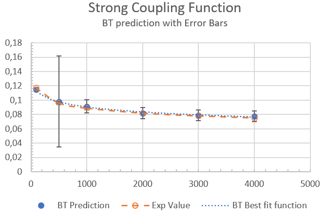
Considering the best fit function of the theoretical data in Figure 3b, one obtains an enough precise function with within the energy scale range 92.200 GeV – 4000 GeV
the Eq. (25) is able to interpolate the strong coupling values on the running function. The curve (25) is shown in Figure 4. Its best correspondence with the best fit function obtained by the experimental data
with , confirms the excellent correspondence of the theoretical strong coupling values with the experimental ones, allowing us to suggest an electromagnetic nature of the origin of the strong interaction at each energy scale value.
9. Discussion and Conclusions
The results reported here provide the first fully theoretical prediction of within a framework entirely distinct from QCD, yet achieving excellent agreement with experimental data across multiple energy scales. In fact, this work presents a theoretical prediction of the strong coupling constant as a function of energy scale, developed entirely within the framework of Bridge Theory (BT). Applying the concept of electromagnetic dipole interaction (DEMS) between quarks, the running behaviour of emerges naturally from considerations on the field geometry of the DEMS and energetics, without invoking specific postulates of QCD.
The resulting coupling function, derived from the electromagnetic interaction geometry of quark pairs, exhibits a maximum value at low energy and decreases with increasing scale, reproducing the expected asymptotic freedom. Equation (22), formulated from first principles, enables the calculation of for any energy scale by considering the number of active quarks and exchanged gluons and photons during the interaction of the particles. The theoretical predictions match remarkably well with experimental values across the 91–4000 GeV range, as demonstrated in Table 1 and Figure 3 and Figure 4.
This agreement is particularly striking given that no QCD formalism is used. Instead, the BT formalism interprets strong interactions as emergent from high-intensity electromagnetic couplings between fractional charges, localized through DEMS. The fit function obtained from the BT model closely mirrors the empirical best fit for , confirming the predictive power of the approach.
These results support the hypothesis that the strong force may be an effective manifestation of electromagnetic interactions under specific geometric constraints, and that the coupling constant derives from the same fundamental action principles that govern electromagnetic interactions.
This reinterpretation opens a possible unification path between the strong and electromagnetic interactions without introducing new interaction types, suggesting that the distinction between forces may arise from the interaction scale and dipole structure rather than from fundamentally different fields.
Future investigations will aim to extend this analysis to other processes and energy regimes, and to derive the dynamics of confinement and hadronization within this unified framework.
References
- Jackson, J.D., Classical Electrodynamics, Wiley, New York (1962).
- Auci, M.; Dematteis, G. An approach to unifying classical and quantum Electrodynamics. Int. Journal of Modern Phys. B 1999, 13, 1525. [Google Scholar] [CrossRef]
- Auci, M. Superluminality and Entanglement in an Electromagnetic Quantum-Relativistic Theory. Journal of Modern Physics 2018, 9, 2206–2222. [Google Scholar] [CrossRef]
- M. Auci. “A conjecture on the physical meaning of the transversal component of the pointing vector”. Phys. Lett. A 135, 86 (1989). [CrossRef]
- M. Auci. “A conjecture on the physical meaning of the transversal component of the Poynting vector. II. Bounds of a source zone and formal equivalence between the local energy and the photon.” Phys. Lett. A 148, 399 (1990). [CrossRef]
- M. Auci. “A conjecture on the physical meaning of the transversal component of the Poynting vector. III. Conjecture, proof and physical nature of the fine structure constant”. Phys. Lett. A 150, 143 (1990). [CrossRef]
- Auci, M. Estimation of an absolute theoretical value of the Sommerfeld’s fine structure constant in the electron–proton capture process. Eur. Phys. J. D 2021, 75, 253. [Google Scholar] [CrossRef]
- Auci, M. On a Non-Standard Atomic Model Developed in the Context of Bridge Electromagnetic Theory. Journal of Physical Chemistry & Biophysics 2024, 14 5, 1-13. [CrossRef]
- Morel, L., Yao, Z., Cladé, P. et al. Determination of the fine structure constant with an accuracy of 81 parts per trillion. Nature 588, 61-65 (2020). [CrossRef]
- The DELPHI Collaboration., Abreu et al., P. Consistent measurements of αs from precise oriented event shape distributions. Eur. Phys. J. C 14, 557–584 2000. [CrossRef]
- d’Enterria et al. “The strong coupling constant: state of the art and the decade ahead”. J. Phys. G: Nucl. Part. Phys. 51 (2024) 090501. [CrossRef]
- S. Navas et Al. (Particle Data Group Collaboration). “Review of Particle Physics”. Phys. Rev. D 110, 030001, (2024). [CrossRef]
Figure 1.
(a) The action function is obtained by the overlapping of two contributes, the electrostatic dominating for and electromagnetic dominating for , with , which value has been calculated using a MAPLE algorithm. In the DEMS interval , the dipole ratio has a root-mean-squared value to which corresponds the Planck action value. (b) The coupling function shows the maximum value of coupling in correspondence of the minimum of action of the interacting system. The interval of the dipole ratio associated to the strong interaction is limited in the range . For the electrostatic interaction is dominating. Therefore, the value of the strong coupling constant cannot be unique but variable according to the energy scale (renormalisation energy) of the interaction that acts on the length of the dipole moment of the DEMS and its corresponding wavelength. This variability of the coupling value represents what is referred to in QCD as “running coupling”.
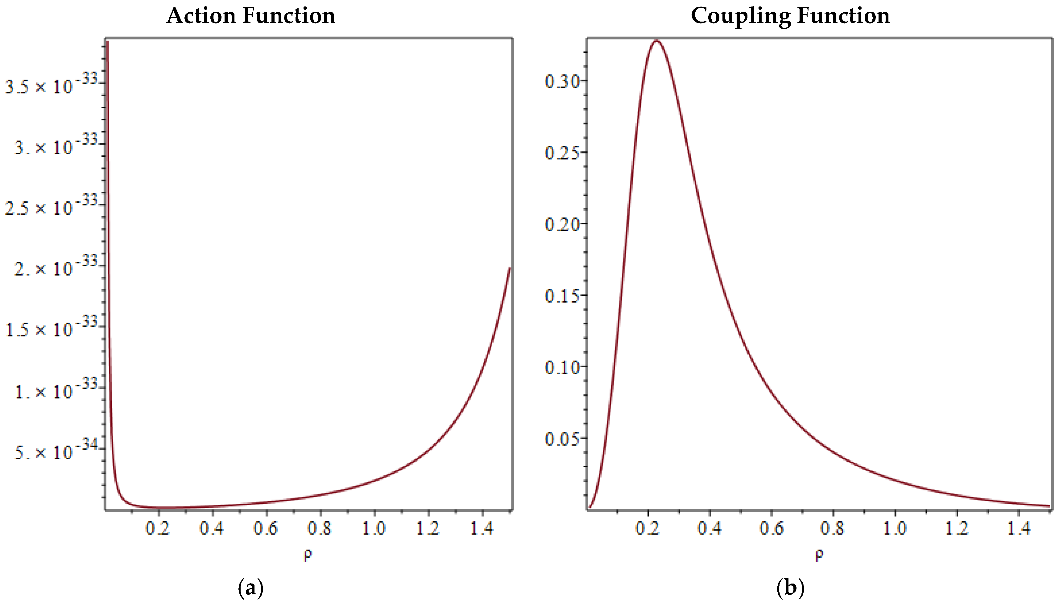
Figure 2.
the complete coupling function is shown as the dipole ratio varies for a pair of interacting quarks. The zone limited by the interval correspond to the “running coupling” range in QCD.
Figure 2.
the complete coupling function is shown as the dipole ratio varies for a pair of interacting quarks. The zone limited by the interval correspond to the “running coupling” range in QCD.
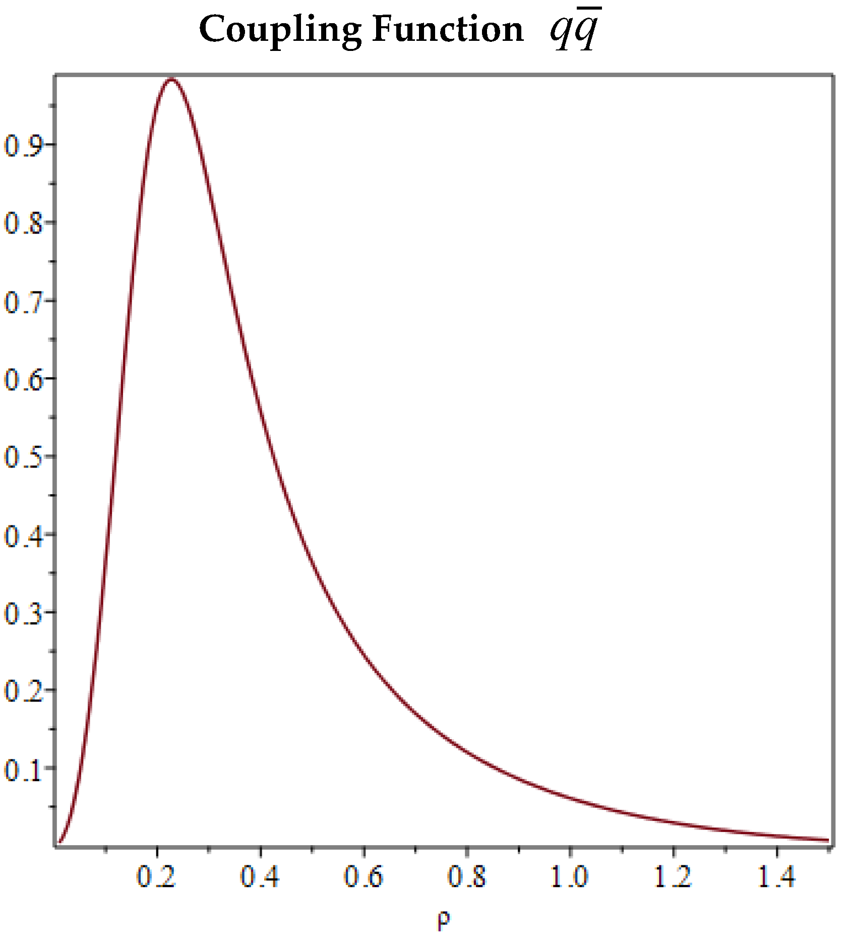
Figure 3.
(a) representation in blue diamonds of the experimental measures of the strong coupling constants at different values of energy scale. The phenomenon of the coupling constant variation in QCD is defined “running coupling” and refer to the way the strength of fundamental forces in particle physics varies with the energy scale at which they are measured. (b) representation in hollow red diamonds of the theoretical results in Table 1, expressed as an average of the values of the coupling constant calculated for each production channel involved at a given energy scale. (c) representation of the superposition (a) + (b). (d) representation of the data in (c) and relationship with the curves obtained from Eq. (22) before being mediated.
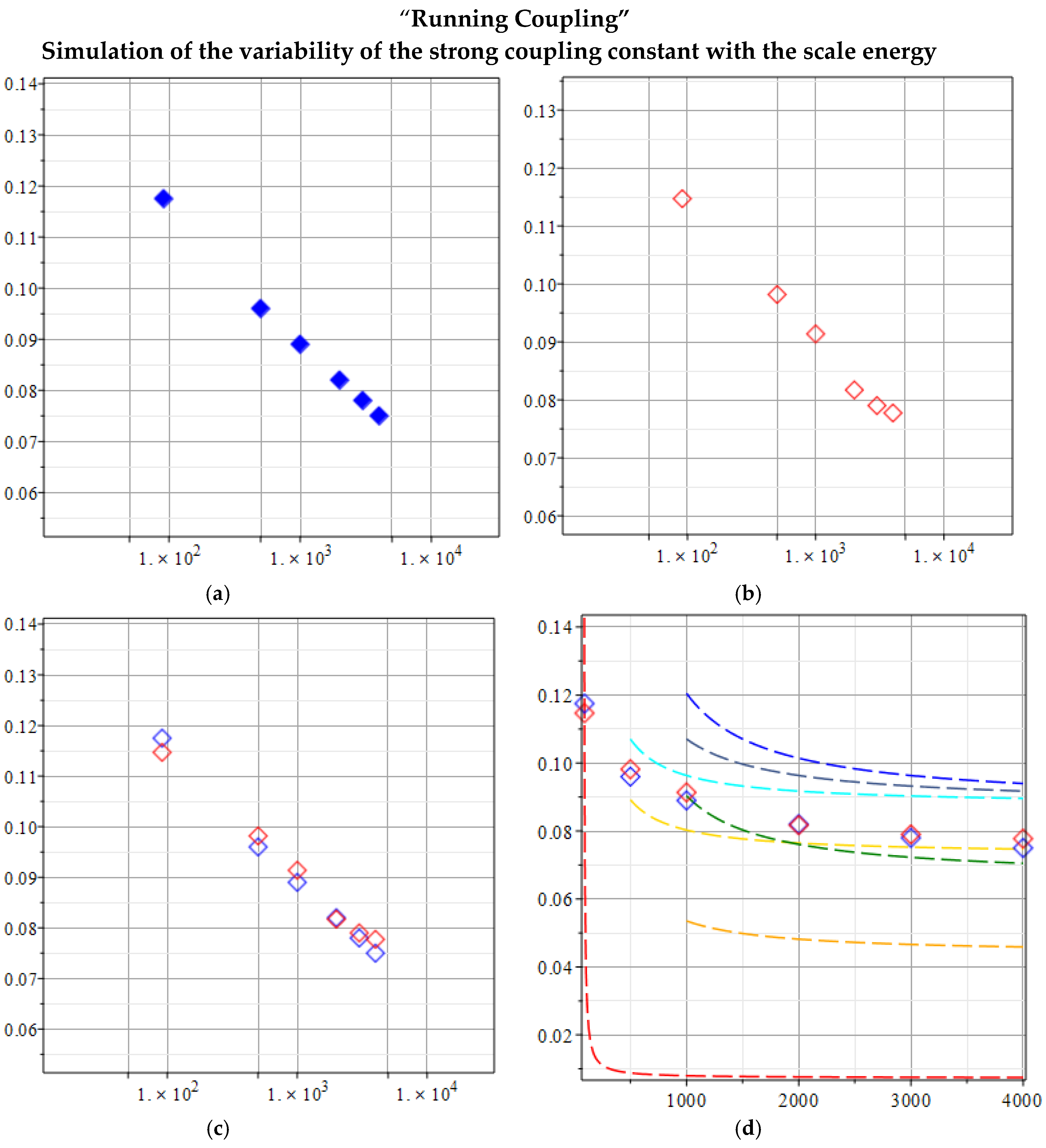
Figure 4.
shows the data of the strong coupling value of Figure 3c with the relative statistical errors reported in Table 1 due to the superimposition of measurements from curves obtained from different production channels, it is evident the typical behaviour due to the running coupling in the interval 91-4000 GeV.
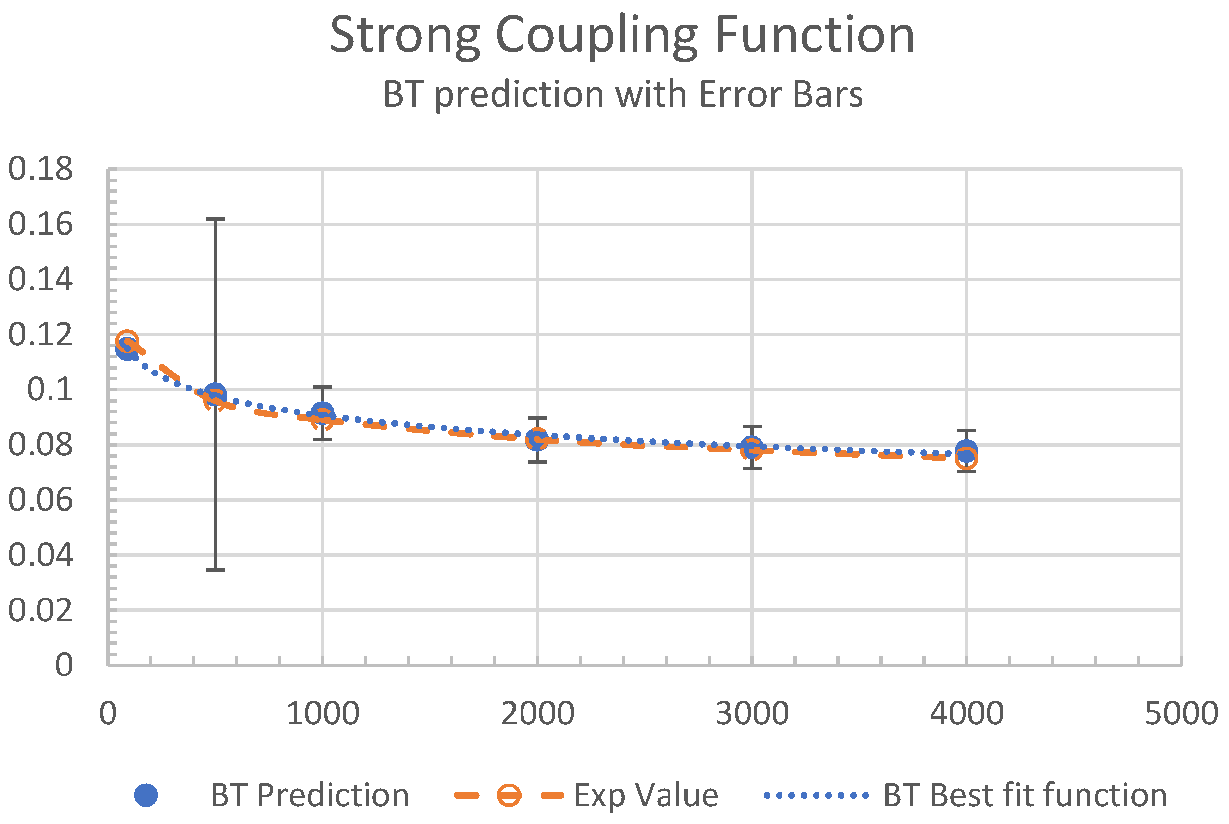

Table 1.
The Strong Coupling Constant as a Function of the Energy Scale .
| (GeV) | (GeV) | |||||||||
| (*) | 2 | 1 | 0 | 91.200 | 0.9365 | 91.1880 | 0.1147 | 0.1147 | - | 0.1175[10-12] |
| Contributes | ||||||||||
| 5 | 1 | 0 | 500 | 1 | 91.1880 | 0.8925 | Average | |||
| 3 | 1 | 3 | 500 | 1 | 91.1880 | 0.1071 | 0.09817 | 0.06374 | 0.096[12] | |
| Contributes | ||||||||||
| 5 | 1 | 0 | 1000 | 1 | 91.1880 | 0.08029 | Average | |||
| 3 | 2 | 0 | 1000 | 2 | 91.1880 | 0.05355 | ||||
| 3 | 3 | 0 | 1000 | 3 | 91.1880 | 0.09041 | ||||
| 3 | 1 | 3 | 1000 | 1 | 91.1880 | 0.09635 | ||||
| 3 | 1 | 3 | 1000 | 2 | 91.1880 | 0.1071 | ||||
| 3 | 1 | 3 | 1000 | 3 | 91.1880 | 0.1205 | 0.09137 | 0.00945 | 0.089[12] | |
| Contributes | ||||||||||
| 5 | 1 | 0 | 2000 | 1 | 91.1880 | 0.07646 | Average | |||
| 3 | 2 | 0 | 2000 | 2 | 91.1880 | 0.04818 | ||||
| 3 | 3 | 0 | 2000 | 3 | 91.1880 | 0.07608 | ||||
| 3 | 1 | 3 | 2000 | 1 | 91.1880 | 0.09175 | ||||
| 3 | 1 | 3 | 2000 | 2 | 91.1880 | 0.09635 | ||||
| 3 | 1 | 3 | 2000 | 3 | 91.1880 | 0.1014 | 0.08171 | 0.00793 | 0.082[12] | |
| Contributes | ||||||||||
| 5 | 1 | 0 | 3000 | 1 | 91.1880 | 0.07526 | Average | |||
| 3 | 2 | 0 | 3000 | 2 | 91.1880 | 0.04662 | ||||
| 3 | 3 | 0 | 3000 | 3 | 91.1880 | 0.07227 | ||||
| 3 | 1 | 3 | 3000 | 1 | 91.1880 | 0.09031 | ||||
| 3 | 1 | 3 | 3000 | 2 | 91.1880 | 0.09324 | ||||
| 3 | 1 | 3 | 3000 | 3 | 91.1880 | 0.09635 | 0.07901 | 0.00761 | 0.078[12] | |
| Contributes | ||||||||||
| 5 | 1 | 0 | 4000 | 1 | 91.1880 | 0.07468 | Average | |||
| 3 | 2 | 0 | 4000 | 2 | 91.1880 | 0.04588 | ||||
| 3 | 3 | 0 | 4000 | 3 | 91.1880 | 0.07050 | ||||
| 3 | 1 | 3 | 4000 | 1 | 91.1880 | 0.08961 | ||||
| 3 | 1 | 3 | 4000 | 2 | 91.1880 | 0.09175 | ||||
| 3 | 1 | 3 | 4000 | 3 | 91.1880 | 0.09400 | 0.07773 | 0.00748 | 0.075[12] | |
(*) In this low-energy case, not all products are Z bosons, as scattering and annihilation can occur, so estimating that 93.65% of collisions produce a Z boson, we get the tabulated results.
Disclaimer/Publisher’s Note: The statements, opinions and data contained in all publications are solely those of the individual author(s) and contributor(s) and not of MDPI and/or the editor(s). MDPI and/or the editor(s) disclaim responsibility for any injury to people or property resulting from any ideas, methods, instructions or products referred to in the content. |
© 2025 by the authors. Licensee MDPI, Basel, Switzerland. This article is an open access article distributed under the terms and conditions of the Creative Commons Attribution (CC BY) license (http://creativecommons.org/licenses/by/4.0/).
Copyright: This open access article is published under a Creative Commons CC BY 4.0 license, which permit the free download, distribution, and reuse, provided that the author and preprint are cited in any reuse.


