
Submitted:
19 June 2025
Posted:
20 June 2025
You are already at the latest version
Abstract
We investigated the dispersal ability of Euphydryas aurinia provincialis in a local scale analysis within a single habitat patch of the Colfiorito highlands metapopulation. Our findings indicate that inside a single node, the organization of nesting patches can be conceptualized as a metapopulation itself, where reproductive sites, despite their spatial proximity, can act as either source or sink habitats depending on environmental conditions. We conducted fieldwork in six nesting patches inside a single node, capturing, marking, and recapturing individuals to assess their spatial distribution and movement tendencies at large landscape scale. We found a high degree of site fidelity among individuals, with many recaptures occurring within the original marking site but also a sex-based differences in movement patterns; females dispersed farther than males, likely driven by reproductive strategies, while males remained more localized, prioritizing mate-searching. Our findings suggest a complex dynamic in habitat connectivity: pastures and abandoned fields, despite being open, seem to act like a sink areas and breeding sites with shrub and tree cover act as source habitats, offering optimal conditions for reproduction. Individuals, especially females, from these source areas were later compelled to disperse into open habitats, highlighting a nuanced interaction between landscape structure and population dynamics. These results highlight the importance of maintaining habitat corridors to support metapopulation dynamics and prevent genetic isolation; the abandonment of traditional grazing practices is leading to the rapid closure of these source habitats, posing a severe risk of local extinction. Conservation efforts should prioritize the preservation of these source habitats to ensure the long-term viability of E. a. provincialis populations in fragmented landscapes.
Keywords:
marsh fritillary
; lepidoptera
; spatial analysis
; dispersal ability
; ecological network
1. Introduction
In Italy, Euphydryas aurinia is considered a species complex of three taxa: i) aurinia (Rottemburg, 1775), ii) glaciegenita (Verity, 1928) and iii) provincialis (Boisduval, 1828), alternatively considered as species or subspecies by different authors [1,2,3,4,5,6,7]. Euphydryas aurinia provincialis is limited to the Maritime Alps and the Apennine Mountains [8]. It is widespread on the Central Apennines, mostly on Monti Reatini [9] and it has been categorised as “Least Concern” in the recent Red List of Italian Butterflies [10,11]. Studies on this species have focused on several aspects of biology, on larval host plant preference [13], predators [14] and parasitoids [15], adult population dynamics, courtship, and mating behaviour [9].
Marsh fritillary is a univoltine species, with adults emerging from late April to mid-June; females lay up to 300 eggs annually on the underside of the leaves of the larval host plant, particularly Knautia purpurea, Succisa pratensis and Scabiosa columbaria [13,16,17]. These plants are critical for larval development, providing essential nutrition during the early growth phases. From late July, first-instar larvae form communal silken nests that provide stability and protection, with larvae from different oviposition events often aggregating [13]. This gregarious feeding behaviour continues until September-October across four developmental instars. As conditions worsen, larvae individually enter diapause in underground hibernacula (~1 cm3, 25 cm deep) [13]. In early spring, they regroup to resume feeding through the fifth and sixth instars, shifting to solitary dispersal for optimal food access before pupating under dead leaves or grass stems [13].
It is a species particularly linked to pasture environments; a remarkably high grazing pressure characterized the pastoral landscape for centuries, but the last decades have seen a marked trend of grazing cessation and mountain farming abandonment, and thus several sectors are currently abandoned and undergoing vegetation recovery and dynamic processes. Bonelli et al. (2011) [12] documented the extinction of 12 populations of E. aurinia due to habitat destruction and the marsh fritillary suffers a severe decline in most European countries during the twentieth century [18 ‒ 17]. Its presence is therefore essentially linked to a type of extensive agriculture and a good management of pastures and grasslands, especially in mountainous areas. Anyway, the conservation status of the Mediterranea and Alpine population is “favourable” [5‒6], but the risk of a severe decline remains very high, especially if the current management trend of the Apennine Mountain landscape were to be maintained.
Dispersal strategies in E. aurinia complex vary depending on habitat structure and resource distribution [5]; during early instars, movement is limited, with larvae remaining within their natal patches. However, in later instars, particularly the fifth and sixth, larvae exhibit greater mobility, actively dispersing in search of more abundant or higher-quality food sources. The availability of host plants such as Knautia purpurea is a key determinant of larval survival, with patch connectivity playing a crucial role in metapopulation dynamics. Fragmented landscapes may increase dispersal distances, exposing individuals to higher predation risk and environmental stressors. However, well-connected patches facilitate successful movement between resource-rich areas, ensuring higher survival rates and genetic exchange between populations [6]. The source-sink dynamics observed in E. aurinia populations suggest that some patches function primarily as sources, where high larval survival and dispersal rates contribute to the maintenance of adjacent subpopulations. Conversely, sink patches rely on immigration to sustain population numbers, highlighting the importance of habitat connectivity in conservation planning [6].
In our study we investigate on a local scale the dispersal ability of E. a. provincialis population; the analysis focused within a single patch of the more complex ecological network of the Colfiorito highlands (Umbria, central Italy) to understand in detail how it is ecologically structured and if a single patch behaves like a small metapopulation. Warren (1994) [16] suggests that thought to be a sedentary butterfly [19,20,21,22], E. aurinia is probably much more mobile with a suggested colonization range of 15–20 km [23]. We believe that the knowledge of the movements of a species on a fine scale can help to know how a population patch is structured and to have more information on the large-scale dispersal abilities, its extinction risk, recolonization, or the degree of geographical isolation.
2. Material and Methods
2.1. Study Area
Fieldwork was carried out in the highlands of Colfiorito (central Italy) on Mount Orve (950 m a.s.l Lat 43.024951° N; Long 12.883909° E; UTMWGS84) (Figure 1). The Colfiorito plateau system, located in the eastern part of the Umbria region near the Marche region border, comprises seven plains known as: Annifo, Arvello, Colfiorito, Colfiorito marsh, Popoli and Cesi, Colle Croce, and Ricciano. These plateaus lie at altitudes between 700-800 meters above sea level and are bordered to the east and west, by two limestone mountain ridges, reaching elevations of 1,571 m (Mt. Pennino) and 1,405 m (Mt. Tolagna) respectively. The inner landscape is characterized by rolling hills [24]. The catchment basin spans 9,152 hectares and encompasses portions of the Umbria-Marche Apennine. It is the result of ancient lake systems that were gradually drained through both anthropogenic interventions and natural geomorphological processes [25]. A key ecological feature of the area is the Colfiorito marsh, whose value has been recognized at international level. In 1977, the marsh was designated as a Wetland of International Importance under the Ramsar Convention. Furthermore, it has been included in the EU Natura 2000 as both a Special Protection Area (SPA) under the “Birds Directive” 79/409/EEC and a Site of Community Importance (SCI) under the “Habitats Directive” 92/43/EEC respectively [24].
Information on the distribution of E. a. provincialis in the Colfiorito highlands was provided by Salomone et al., (2010) [26]. A UTM WGS84 rectangular grid was superimposed over the entire plateau system (Figure 1A), and for each grid cell, presence/absence of the species was recorded. The species was detected in 17 out of 50 grid cells (about 34%). For this study, we selected the grid cell located closest to the centroid of the species’ dispersal nodes (Figure 1B) and conducted a complete census of E. a. provincialis larval nests. The selected grid cell covers an area of 235.5 hectares and includes a mosaic of different land uses: close -turf grassland, uncultivated fields, forest patches and cultivated fields (Table 1). Changes in traditional land management practices have led to the expansion of shrublands, leading to a remarkable modification of ecosystem services and biodiversity. The study area lies within the temperate bioclimatic region, and it is characterized by the alternation of winter cold stress and summer drought stress, with different intensities, depending on the elevation gradient and landform factors [27].
2.2. Experimental Design and Data Collection
Field research was conducted from September to October 2008, resulting in the detection of 46 nests organized into six nesting patches within the study area. For each nest, the geographical coordinates (UTM, WGS84), host plant species and number of observed larvae were recorded. Each nesting patch was obtained using the minimum convex polygon algorithm [28], starting from the position of each nest. The centroid of each minimum convex polygon was then obtained (Figure 1C). The centroid of the minimum convex polygon (nesting patch) represents the origin of a 150 meters radius buffer (Figure 1D), i.e., the mark release recapture area (MMRA). Each MRRA (7.1 hectares) was picketed and divided into four -quadrants (NE, SE, SW, NW). Capture sessions were carried out from May 4th to June 10th, 2009, with two visits per week for a total of 10 surveys. In each session, all six MRRA were surveyed simultaneously, with a sampling effort of 45 minutes per quadrant. During these surveys, the GPS positions of marked or recaptured individuals were recorded, along with their food preferences and sex. The marking procedure followed the method described by Ehrlich and Davidson (1960) [29], as modified by Brussard (1971) [30] and outlined in Southwood (1978) [31]. Individuals were marked on the ventral surface of the wings, waterproof pens, with a different colour assigned to each patch (Figure 2).
2.3. Statistical Analysis
To assess the uniformity of capture, marking, and recapture efforts among patches, a Kruskal-Wallis test [32] was employed. This non-parametric method is suitable for comparing independent groups when the assumption of normality is not met.
Geographic distances were calculated using QGIS software (version 3.28.15) as Euclidean distances between the centroid of nesting patches, or between the coordinates of individual marking and recapture events. Differences in dispersal distances between males and females were tested using the Wilcoxon rank-sum test [33], a non-parametric alternative to the t-test for independent samples.
Differences in dispersal among patches were analysed using the Kruskal-Wallis test (Kruskal & Wallis, 1952), which allows comparisons among multiple groups without assuming normality. To test the relationship between dispersal distance and time since marking, Hoeffding’s D test [34] was used, a non-parametric statistic capable of detecting both linear and non-linear dependencies. To assess monotonic relationships, Kendall’s tau correlation coefficient [35] was used, offering a rank-based approach that is more robust to non-normal data distributions and outliers.
Site fidelity was assessed using chi-square (χ2) tests to test for independence between site fidelity and sex, and between site fidelity and patch location.
Patch connectivity was quantified using graph theory metrics [36,37,38,39]. Degree centrality measures the number of direct connections to each patch and indicates whether patches are dispersal hubs or isolated. Betweenness centrality highlights patches that act as key dispersal corridors and are crucial for maintaining network connectivity. Closeness centrality evaluates the overall efficiency with which a patch can reach the rest of the network, reflecting its integration within the dispersal system. Together, these metrics provide a comprehensive understanding of the function of the patches within the dispersal network, supporting conservation efforts that target both well-connected and peripheral patches. To assess the spatial structure of patch connectivity, Moran’s I test [40] was used to evaluate whether the degree centrality of patches exhibited spatial autocorrelation. The test was conducted under a randomization framework, with a spatial weight’s matrix constructed based on the nearest neighbours. To investigate the influence of geographic distance on patch connectivity further, a Mantel test [41] was performed to assess the correlation between the geographic distance matrix and the connectivity matrix (degree centrality).
Nine parameters were collected for the environmental analysis using QGIS 3.28.15 geoprocessing tools. For each nesting patch buffer (MRRA) the vegetation and geomorphological parameters (slope, exposure and distance from the hydrographic network) were measured. Vegetation parameters were collected entirely through field surveys and expressed as a proportion (p) of the available habitat in the study area. Vegetation types were first identified and categorized in the field based on their physiognomy (pre-wooded community, shrubland, grassland, meadow, marsh and hydrophytic vegetation, cropland). Then, some of these categories were described in more detail based on the vegetation structure and dominant species. Multivariate factorial analysis [42] was applied to investigate changes in environmental parameters in relation to the ecological role of each nesting patch (source or sink). Factorial analysis was performed on the correlation matrix, and the results are presented as biplots.
All statistical analyses were performed in RStudio [43] (R Core Team, 2024 [44]), using various packages: the stats for Wilcoxon rank-sum, Kruskal-Wallis, Kendall’s tau correlation, and chi-square tests; the Hmisc package for Hoeffding’s D test; the igraph package for calculating graph-theory connectivity metrics; the ape package for the Moran’s I index; and the vegan package for the Mantel test. The significance level was set at α = 0.05 for all tests.
3. Results
3.1. Mark Release Recapture Results
Field surveys conducted from September to October 2008 identified a total of 46 larval nests, distributed across six distinct nesting patches (Figure 1D). The number of nests per patch varied, ranging from five to nine, with an average of 7.7 nests per patch (SD = 1.5) (Table 2). Geographical coordinates (UTM, WGS84), host plant species, and the number of larvae observed were recorded for each nest. The concentration of nests in certain patches suggests that some areas within the landscape provide more suitable microhabitats for larval survival.
During the mark-recapture field surveys conducted in May-June 2009, a total of 3,253 individuals were marked (Table 2), with 151 recaptures (91 males; 60 females), resulting in an overall recapture rate of 4.6%. Recapture rates varied among the patches, ranging from 2.5% in patch 4 to 6.0% in patches 1 and 2. The highest number of marked individuals was recorded in patch 5 (731 butterflies), whereas patch 6 had the lowest marking effort (436 butterflies). On average, 542.2 individuals were marked per patch, with a mean recapture count of 25.2 butterflies per patch. The Kruskal-Wallis test evaluating differences in capture rates across patches was not statistically significant (χ2 = 3.0745, df = 5, p = 0.688) and for recapture effort (χ2 = 3.304, df = 5, p = 0.653). This suggests that despite the numerical differences, the effort involved in capture, marking and recapture was homogeneous among sites and between sexes.
Most of the adults were captured on Thymus longicaulis longicaulis, which accounted for 44.02% of all the recorded observations made (n = 1432) followed by Hippocrepis comosa (22.65%, n = 737). Several other plant species were recorded at lower frequencies, including Sanguisorba minor (2.56%, n = 83) and Taraxacum officinale (1.78%, n = 58). Other species such as Acinos alpinus (8.55%, n = 278) and Crepis sancta (6.41%, n = 208), also contribute significantly to the presence of adults (Figure 3). Knautia purpurea, known as a key larval host plant, was only marginally represented in adult captures (0.48%, n = 16), suggesting that adults do not frequently use it as a nectar source.
3.3. Descriptive Statistics of Dispersal Distances
The dispersal distances of recaptured E. a. provincialis individuals ranged from 5.4 to 740.0 meters, with a mean distance of 149.3 m (SD = 132.3 m; CV= 73.2–171.7 m) and a median value of 120.0 m. When analysed by sex, substantial differences in dispersal distances were observed (Figure 4): females exhibited greater dispersal distances (mean = 204.7 ± 176.6 m; CV= 89.1–256.7 m) compared to males (mean = 107.5 ± 57.1 m; CV= 68.6–138.9 m) (Table 3).
The Wilcoxon test confirmed that these differences were statistically highly significant (W = 1858.6, p < 0.000), indicating that females tended to disperse significantly farther than males. However, the Kruskal-Wallis test assessing whether dispersal distances varied among patches was not statistically significant (χ2 = 5.51, df = 5, p = 0.360), suggesting that dispersal distances are consistent across different patches.
Overall, site fidelity is high, with 89.4% of individuals being recaptured in their initial patch. However, there was a notable difference between the sexes: males exhibited significantly higher site fidelity (98.8%) than females which displayed a lower site fidelity (76.9%). The χ2 test indicates that site fidelity differs significantly between the sexes (χ2 = 16.525, df = 1, p < 0.000). The χ2 test evaluating differences in site fidelity across patches was not statistically significant (χ2 = 6.74, df = 5, p = 0.240), suggesting that there is no significant variation in site fidelity among different patches.
Hoeffding’s D test [34] was used to assess the general dependency between the number of days elapsed since marking and the dispersal distance of E. a. provincialis. The test revealed a very weak correlation (D = 0.01) between the two variables in the overall dataset and the observed p-value (0.035) was statistically significant, suggesting that the dependency is unlikely to be due to chance (Figure 5). However, the extremely low D value indicates that the relationship between the two variables is biologically negligible. When analysed separately for males and females, different patterns emerged: males showed no correlation between day and dispersal distance (D = 0.00, p = 0.5699), indicating that these two parameters are independent on each other; females, on the other hand, exhibited a slightly higher correlation (D = 0.02, p = 0.026), which was statistically significant but still weak. This suggests that dispersal distance increases with time more in females than in males, although the effect remains small. The direct comparison (Figure 5) between male and female Hoeffding’s D values showed a minor difference (ΔD = -0.023), indicating that females have a slightly stronger dependency between days and dispersal distance, but this difference remains small, and the effect size is minimal.
The analysis of the relationship between days since marking and dispersal distance, separated by sex and capture patch, revealed some notable differences (Figure 6). For male the Hoeffding’s test [34] revealed no significant dependence for all patches, the number of days does not influence dispersal distances. In females, we only find a significant dependence (D=0.1, p= 0.022) between days and dispersal distance over time in patch 5, while in other patches, days and dispersal are not correlated. In patches 5 and 3 (source zones), the greater the number of days, the greater the dispersal distance of the females.
3.4. Patch Connectivity Network
The dispersal dynamics of E. a. provincialis were analysed to determine whether specific patches predominantly acted as sources (emitting more individuals than they receive) or sinks (receiving more individuals than they emit). The dispersal balance for each patch was calculated as the difference between emigrants and immigrants, where positive values indicate source patches and negative values indicate sink patches (Table 4). The results reveal that patches do not function equally in terms of dispersal. Certain patches act as primary contributors to population connectivity, while others primarily receive individuals from neighbouring patches.
Patches do not have the same ecological role in the dispersal network (Table 5). Patch 2 emerges as the most connected and central node, exhibiting the highest degree centrality (7 connections) and betweenness centrality (8), indicating its function as a key dispersal hub or even a “super-source.” It interacts with multiple patches and maintains good proximity to others (closeness = 0.125), thereby reinforcing its role in facilitating movement across the network (Figure 7). In contrast, patch 6 exhibits the least influential, showing localized movements without broader connectivity and does not act as a link between other patches, emphasizing its peripheral role in the network (Figure 7). Patch 5, on the other hand, exhibits the highest proximity and closeness centrality (0.143), suggesting well-distributed connectivity within the network and a moderate bridging role (betweenness = 4). This patch likely represents a central hub with balanced dispersal flows (Figure 7). Patch 1 appears to be the most peripheral, functioning as a probable sink patch with limited interactions and low connectivity. It is the most spatially isolated from other patches, displaying the lowest closeness centrality (0.071) and connectivity function (betweenness = 3).
To assess whether a patch’s connectivity influences the time elapsed since marking, Kendall’s tau correlation was performed between patch connectivity and dispersal days. The results (tau = 0.4348, p = 0.045) indicate a moderate positive correlation, suggesting that patches with higher connectivity are more likely to be involved in dispersal events occurring over longer periods. Some patches consistently maintain a source function over time, acting as stable points in the dispersal network and the relationship is statistically significant, confirming that connectivity influences dispersal patterns.
These patterns suggest a strong relationship between the spatial position of patches (Figure 1D) and their role in the dispersal network. Moran’s I test [40] was conducted to evaluate whether the degree of centrality of the patches is spatially structured (Table 6). The results yielded a negative Moran’s I value (-0.068), suggesting a potential tendency toward spatial dispersion rather than clustering. However, the p-value (0.275) indicates that this pattern is not statistically significant, meaning that the observed spatial distribution of connectivity could have occurred by chance. Under the assumption of spatial randomness, the expected Moran’s I value was -0.200 and the observed value I was lower than this, yet the standard deviation (0.598) does not exceed the critical threshold for significance. These results suggest that highly connected patches are not necessarily spatially clustered, and that patch connectivity does not appear to follow a clear geographic pattern. This implies that the role of a patch within the dispersal network is not strongly dictated by its physical location, and that other ecological and environmental factors, such as habitat quality, patch size, or species-specific movement behaviour, may play a more significant role in determining connectivity.
To further assess the relationship between geographic proximity and connectivity, a Mantel test (Mantel, 1967) was performed to compare the geographical distance matrix with the connectivity matrix (degree centrality). The test yielded a negative Mantel statistic (0.015), indicating a weak inverse correlation: patches that are farther apart tend to have different connectivity levels (Table 6). However, this relationship was not statistically significant (p = 0.417), meaning there is no strong evidence that connectivity decreases with geographic distance. The null model, based on 719 permutations, showed that the observed correlation falls well within the expected range under random conditions This further supports the conclusion that spatial distance alone does not determine patch connectivity.
Principal Component Analysis (PCA) was conducted to determine the key environmental factors influencing the classification of patches as either source or sink. The first two principal components (PC1 and PC2) explain 78.4% of the total variance, with PC1 accounting for 44.2% and PC2 for 34.2% (Figure 8); PC1 is highly correlated with open pastures (0.91), closed pastures (0.93), and abandoned cultivated lands (0.44), representing a gradient from open to closed landscapes. Meanwhile PC2 is mainly influenced by ruderal vegetation (0.81), urban areas (0.92), and abandoned fields (-0.82), indicating a gradient of anthropogenic influence (Table 7). These findings align with Moran’s I test and Mantel test (Table 6), which suggested that highly connected patches are not necessarily spatially clustered, and patch connectivity does not follow a clear geographic pattern. Instead, ecological and environmental factors, such as land use or vegetation, seem to play a more significant role in shaping patch connectivity.
The distribution of PCA scores reveals a clear distinction between source and sink patches (Figure 8), with source patches (2, 3, and 5) tending to have negative PC1 scores, indicating an association with ruderal vegetation and cultivated areas, and sink patches (1, 4, and 6) displaying a positive PC1 values, suggesting a preference for open pastures and abandoned fields (Table 7). The second component does not differentiate significantly between source and sink patches, which reinforces the idea that their ecological role is determined by landscape structure rather than anthropogenic influence. A Welch Two Sample t-test confirms that PC1 scores differ significantly between source and sink patches (p = 0.025, Table 8), indicating that this axis effectively separates the two groups. Conversely, PC2 does not show a statistically significant difference (p = 0.636), supporting the idea that anthropogenic factors are not the main drivers of patch function.
4. Discussion
Our study on E. a. provincialis dispersal dynamics highlights critical insights into the species’ movement patterns and habitat use, with important implications for its conservation. As previously discussed in the introduction this species is highly dependent on semi-natural grasslands, which are increasingly threatened by land-use changes, particularly the abandonment of traditional pastoral practices.
One of the most significant findings of our study is the limited dispersal ability of E. a. provincialis. The dispersal distances observed in recaptured individuals ranged from 5.4 to 740.0 m, with an average of 149.3 m. However, when analysed by sex, females exhibited significantly greater dispersal distances than males, as confirmed by the Wilcoxon test (p < 0.000). This pattern aligns with findings in other butterfly species where females tend to disperse further, likely driven by reproductive strategies requiring exploration of new oviposition sites [23,45,46]. The higher coefficient of variation (CV) in female dispersal distances suggests a broader range of movement strategies, which may be influenced by habitat heterogeneity or resource distribution. Site fidelity was overall high, with 89.4% of individuals recaptured within their original patch. However, a stark contrast between sexes was evident: males exhibited significantly higher site fidelity (98.8%) compared to females (76.9%), as indicated by the chi-square test (p < 0.000). This pronounced difference is consistent with the hypothesis that males prioritize mate-seeking behaviour within a localized area, while females are more inclined to disperse in search of optimal oviposition sites [47].
The relationship between dispersal distance and the number of days since marking was assessed using Hoeffding’s D test. The overall dataset revealed a statistically significant but extremely weak correlation (D = 0.01, p = 0.035), suggesting that while a temporal component exists, its biological relevance is negligible. When analysed by sex, males exhibited no significant correlation (D = 0.00, p = 0.570), indicating temporal independence in their dispersal behaviour. Conversely, females showed a slight but statistically significant positive correlation (D = 0.02, p = 0.026), suggesting that their dispersal distances may increase over time, albeit weakly. This pattern could reflect an incremental search process for suitable oviposition sites, reinforcing the idea that female dispersal is driven by reproductive requirements rather than random movement. However, the direct comparison between male and female Hoeffding’s D values (ΔD = -0.023) underscores the minimal effect size of this difference, indicating that the temporal influence remains marginal in both sexes. In males, Hoeffding’s test consistently found no significant dependence across all patches, reinforcing the conclusion that male dispersal is unaffected by time. In contrast, among females, a significant dependence was observed only in patch 5 (D = 0.1, p = 0.022), while in other patches, no correlation was detected. This localized effect suggests that specific environmental or demographic factors in patch 5 may facilitate increased dispersal over time for females, potentially due to resource depletion or increased competition. The relationship between dispersal distances and time since marking in insects, particularly in Lepidoptera, has been a subject of interest in scientific literature. In this regard, previous studies have shown that some butterfly species exhibit a correlation between the distance travelled and the number of days since marking. For example, research on Parnassius apollo has demonstrated that individuals tend to move over longer distances as time increases, suggesting an exploratory behavior linked to resource or mate searching [48]. However, this relationship is not universal among all butterfly species. In some populations, dispersal distance may be influenced by environmental variables, habitat availability, and species-specific ecological traits [49]. Therefore, while some species exhibit increasing dispersal distances over time, this relationship may be less evident or even absent in others.
The role of individual patches in the dispersal network varies considerably, with some patches acting as sources (emitting more individuals than they receive) and others as sinks (receiving more individuals than they emit). The dispersal balance analysis identified patch 2 as the strongest source patch, while patches 1, 4, and 6 predominantly functioned as sinks. This heterogeneity in dispersal roles suggests that, even on a very small scale, patches are not ecologically equivalent, and some may play a more critical role in maintaining metapopulation connectivity.
Patch connectivity metrics further reinforced these findings, with patch 2 emerging as the most central node in the dispersal network. It exhibited the highest degree centrality and betweenness centrality, indicating its role as a key dispersal hub. Conversely, patch 6 was the least connected, acting as a peripheral and isolated patch. Patch 5 exhibited the highest proximity (closeness centrality), suggesting it may facilitate movement between multiple patches, functioning as an important stepping-stone in the network. These results indicate that dispersal on a large scale is not evenly distributed across the landscape but instead occurs via a structured network in which certain patches act as primary conduits of movement.
Despite the observed differences in connectivity, the spatial distribution of connected patches did not follow a clear pattern. Moran’s I test indicated a lack of spatial autocorrelation in patch connectivity, suggesting that highly connected patches are not necessarily clustered together. Similarly, the Mantel test found no significant correlation between geographic distance and connectivity, indicating that spatial proximity alone does not determine how well-connected a patch is within the dispersal network. This suggests that factors other than simple geographic distance, such as habitat quality, patch size, or species-specific movement preferences, play a more important role in shaping connectivity.
Interestingly, while dispersal distances did not vary significantly among patches, connectivity differences suggest that some patches serve as critical nodes in maintaining movement pathways. The lack of spatial autocorrelation in connectivity suggests that dispersal is not solely dictated by physical proximity but by other ecological factors. Patches that function as key dispersal hubs may do so because of their habitat quality, availability of resources, or interactions with other landscape features that facilitate movement.
These findings are further supported by the Principal Component Analysis (PCA), which identified key environmental factors influencing patch classification as either source or sink. These factors are represented by a gradient from open to closed landscapes and anthropogenic influence. Notably, patches classified as sources (2, 3, and 5) were associated with ruderal vegetation and cultivated areas, whereas sink patches (1, 4, and 6) corresponded to open pastures and abandoned fields. The Welch Two Sample t-test confirmed the PCA results reinforcing the idea that landscape structure determines the ecological function of the patch network.
5. Conclusions
These studies show that the dispersal of the butterfly E. a. provincialis is influenced by a combination of reproductive strategies, mate-seeking behaviours, and specific habitat characteristics. Landscape composition is very important in determining dispersal connectivity. While spatial arrangement alone does not dictate connectivity patterns, habitat type and structural heterogeneity appear to be key factors influencing movement. This suggests that conservation strategies should focus not only on maintaining patch proximity but also on preserving habitat diversity to facilitate dispersal. Understanding these connectivity metrics allows for targeted conservation strategies. The Colfiorito Highlands have undergone significant landscape and economic transformations over time. Originally covered by forest and wetlands, human settlements gradually shaped the terrain through deforestation and drainage effort, promoting agriculture and pastoralism. During the Roman era, infrastructure development boosted trade and crop cultivation. The Middle Ages saw monastic land reclamation and a thriving wool industry. Rural depopulation of the 20th century led to a decline in traditional farming and the strong reduction in grazing has caused a recovery in vegetation dynamism with a consequent closure of prairies, reforestation and an increase of uncultivated areas. These changes pose a significant threat to species strictly dependent on pastures, such as E. a. provincialis, whose habitat is becoming increasingly fragmented into interconnected patches, with a high risk of local extinction. Future research should explore how additional ecological variables, such as resource availability and intra-patch vegetation complexity influence movement decisions in E. a. provincialis. Genetic analyses could provide deeper insights into the factors shaping the dispersal networks
Author Contributions
Brusaferro A: conceptualization, methodology, investigation, data curation, formal analysis, writing—original draft preparation, writing—review and editing. Marinsalti S: conceptualization, methodology, investigation, data curation, visualization, writing—review and editing. Tardella F.M.: investigation, data curation, formal analysis. Insom E.: conceptualization, methodology, investigation, data curation, resources, writing—review and editing, supervision, project administration. La Terza A: conceptualization, resources, writing—review and editing, supervision, project administration. All authors have read and approved the manuscript.
Funding
this research didn’t receive funding.
Acknowledgments
The authors of the article would like to thank the Colfiorito Regional Park staff Dr.ssa Biancarita Eleuteri and Dr.ssa Alessandra Picchiarelli. The group would like to thank Dr. Pietro Salomone for collaboration during the field surveys.
Conflicts of Interest
The authors declare no conflict of interest
References
- Verity, R. Famiglie Apaturidae e Nymphalidae. In: Le Farfalle diurne d’Italia. Marzocco, Firenze, Italy, 1950; Vol. IV, Tav. 38-54, XV-XX, 380 pp.
- Hartig, F. Einige neue Lepidopterenrassen und -formen und eine wiederentdeckte Noctuide aus Süditalien. Reichenbachia, 1968, 12, 1–13. [Google Scholar]
- Prola, C.; Provera, P.; Racheli, T.; Sbordoni, V. I Macrolepidotteri dell’Appennino Centrale. Parte I. Diurna, Bombyces e Sphinges. Fragm. entomol. 1978, 14, 1–217. [Google Scholar]
- Parenzan, P.; Porcelli, F. I Macrolepidotteri Italiani fauna. Lepidopterorum Italiae (Macrolepidoptera). Phytophaga 2006, 15, 1–1051. [Google Scholar]
- Balletto, E.; Cassulo, L.A.; Bonelli, S. . An annotated checklist of the Italian butterflies and skippers (Papilionoidea, Hesperiioidea). Zootaxa (Monograph) 2014, 3853, 1–114. [Google Scholar] [CrossRef] [PubMed]
- Casacci, L.P.; Cerrato, C.; Barbero, F.; Bosso, L.; Ghidotti, S.; Paveto, M.; Pesce, M. , Plazio, E.; Panizza, G.; Balletto, E.; Viterbi, R.; Bonelli, S. (2015). Dispersal and connectivity effects at different altitudes in the Euphydryas aurinia complex. J. Insect Conserv. 2015, 19, 265–277. [Google Scholar] [CrossRef]
- Korb, S.K.; Bolshakov, L.V; . Fric, Z.F.; Bartonova, A. Cluster biodiversity as a multidimensional structure evolution strategy: Checkerspot butterflies of the group Euphydryas aurinia (Rottemburg, 1775) (Lepidoptera: Nymphalidae). Syst. Entomol. 2016, 41, 441–457. [Google Scholar] [CrossRef]
- Balletto, E; Bonelli, S.; Zilli, A. Lepidotteri. In: Angelini, P.; Bianchi, E.; Duprè, E.; Ercole, S.; Giacanelli, V.; Ronchi, F.; Stoch, F.; editors. Specie e habitat di interesse comunitario in Italia: Distribuzione, stato di conservazione e trend. Roma, Italy: Rapporti ISPRA, 2014b, pp. 118–130.
- Pinzari, M.; D’Alessandro, P.; Scalercio, S.; Biondi, M. Make it simple: mating behaviour of Euphydryas aurinia provincialis (Lepidoptera: Nymphalidae). J. Nat. Hist. 2019, 53, 1811–1823. [Google Scholar] [CrossRef]
- Balletto, E.; Bonelli, S.; Barbero, F.; Casacci, L.P.; Sbordoni, V.; Dapporto, L.; Scalercio, S.; Zilli, A.; Battistoni, A.; Teofili, C.; Rondinini, C. Lista Rossa IUCN delle Farfalle Italiane ‒ Ropaloceri. Roma, Italy: Comitato Italiano IUCN e Ministero dell’Ambiente e della Tutela del Territorio e del Mare, 2015, pp. 47.
- Bonelli, S.; Cerrato, C.; Balletto, E. The Red List of Italian Butterflies. In: Rondinini, C.; Battistoni, A.; Peronace, V.; Teofili, C. (Eds.), Italian Red List of Threatened Species. Comitato Italiano IUCN e Ministero dell’Ambiente e della Tutela del Territorio e del Mare, Rome, Italy, 2018, pp. 1–10.
- Bonelli, S.; Cerrato, C.; Loglisci, N.; Balletto, E. Population extinctions in the Italian diurnal lepidoptera: an analysis of possible causes. J. Insect Conserv. 2011, 15, 879–890. [Google Scholar] [CrossRef]
- Pinzari, M.; Pinzari, M.; Sbordoni, V. Egg laying behaviour, host plants and larval survival of Euphydryas aurinia provincialis (Lepidoptera, Nimphalidae) in a Mediterranean population (central Italy). Boll. Soc. entomol. ital. 2016, 148, 12–140. [Google Scholar]
- Pinzari, M. Predation by nymphs of Picromerus bidens (Heteroptera: Pentatomidae) on larvae of Euphydryas aurinia provincialis (Lepidoptera: Nymphalidae). Fragm. entomol. 2016, 48, 131–134. [Google Scholar]
- Pinzari, M.; Scalercio, S.; Brandmayr, P. Associations between the larval-pupal parasitoids Erycia furibunda (Diptera: Tachinidae) and Cotesia bignellii (Hymenoptera: Braconidae) with the butterfly Euphydryas aurinia provincialis (Lepidoptera: Nymphalidae). J. Entomol. Acarol. Res. 2017, 49, 8582. [Google Scholar]
- Warren, M. The UK status and suspected metapopulation structure of a threatened European butterfly, the marsh fritillary Eurodryas aurinia. Biol. Conserv. 1994, 67, 239–249. [Google Scholar] [CrossRef]
- Van Swaay, C.; Collins, S.; Cuttelod, A.; Maes, D. European Red List of Butterflies. Luxembourg: Publications Office of the European Union, 2010; 46 pp. [CrossRef]
- Van Swaay, C.; Warren, M.; Lois, G. Biotope Use and Trends of European Butterflies. J. Insect Conserv. 2006, 10, 189–209. [Google Scholar] [CrossRef]
- Hula, V.; Konvicka, M.; Pavlicko, A.; Fric, Z. Marsh Fritillary (Euphydryas aurinia) in the Czech Republic: monitoring, metapopulation structure, and conservation of an endangered butterfly. Entomol. Fenn. 2004, 15, 231–241. [Google Scholar] [CrossRef]
- Liu, W.; Wang, Y.; Xu, R. Habitat utilization by ovipositing females and larvae of Marsh fritillary (Euphydryas aurinia) in a mosaic of meadows and croplands. J. Insect Conserv. 2006, 10, 351–360. [Google Scholar] [CrossRef]
- Schtickzelle, N.; Choutt, J.; Goffart, P.; Fichefet, V.; Baguette, M. Metapopulation dynamics and conservation of the marsh fritillary butterfly: Population viability analysis and management options for a critically endangered species in Western Europe. Biol. Conserv. 2005, 126, 569–581. [Google Scholar] [CrossRef]
- Fowles, A.P.; Smith, R.G. Mapping the habitat quality of patch networks for the marsh fritillary Euphydryas aurinia (Rottemburg, 1775) (Lepidoptera, Nymphalidae) in Wales. J. Insect Conserv. 2006, 10, 16–177. [Google Scholar] [CrossRef]
- Zimmermann, K.; Fric, Z.; Jiskra, P.; Kopeckova, M.; Vlasanek, P.; Zapletal, M.; Konvicka, M. (2011). Marl Mark-recapture on large spatial scale reveals long distance dispersal in the Marsh Fritillary, Euphydryas aurinia. Ecol. Entomol. 2011, 36, 499–510. [Google Scholar] [CrossRef]
- Orsomando, E.; Catorci, A. Aspetti fitogeografici dei piani. In: Orsomando E (Ed.) Gli altipiani di Colfiorito, Appennino umbro-marchigiano (in Italian). Storia e Ambiente. Tipografia S. Giuseppe, Pollenza, Italy, 1998; 70 pp.
- Orsomando, E.; Pambianchi, G. Carta del paesaggio vegetale del Bacino Imbrifero dell’Altopiano di Colfiorito (in Italian). Università di Camerino. S.EL.CA., Firenze, Italy, 2002.
- Salomone, P.; Insom, E.; Brusaferro, A.; Marinsalti, S. Preliminary study on butterflies of the Colfiorito plateaus: Annifo plain and Colfiorito marsh (Lepidoptera). Boll.Soc.entomol. ital. 2010, 142, 3–20. [Google Scholar]
- Rivas-Martínez, S.; Rivas-Sáenz, S.; Penas, A. Worldwide Bioclimatic Classification System. Glob. Geobot. 2011, 1, 1–634. [Google Scholar]
- Burt, W.H. Territoriality and home range concepts as applied to mammals. J. Mammal. 1943, 24, 346–352. [Google Scholar] [CrossRef]
- Ehrlich, P.R.; Davidson, S.E. Techniques for capture-recapture studies of Lepidoptera populations. J. Lepid. Soc. 1960, 14, 227–229. [Google Scholar]
- Brussard, P.F. Field techniques for investigation of population structure in a “ubiquitous” butterfly. J. Lep. Soc. 1971, 25, 922. [Google Scholar]
- Southwood, T.R.E. Ecological Methods, with particular Reference to the Study of Insect Populations. London, Methuen, UK, 1978. Pp. XVIII + 391.
- Kruskal, W.H.; Wallis, W.A. Use of ranks in one-criterion variance analysis. J. Am. Stat. Assoc. 1952, 47, 583–621. [Google Scholar] [CrossRef]
- Wilcoxon, F. Individual comparisons by ranking methods. Biometrics Bull. 1945, 1, 80–83. [Google Scholar] [CrossRef]
- Hoeffding, W. A Non-Parametric Test of Independence. Ann. Math. Stat. 1948, 19, 546–557. [Google Scholar] [CrossRef]
- Kendall, M.G. A new measure of rank correlation. Biometrika 1938, 30, 81–93. [Google Scholar] [CrossRef]
- Freeman, L.C. A set of measures of centrality based on betweenness. Sociometry 1977, 40, 35–41. [Google Scholar] [CrossRef]
- Freeman, L.C. Centrality in social networks: Conceptual clarification. Social Networks 1978, 1, 215–239. [Google Scholar] [CrossRef]
- Freeman, L.C. Centrality in valued graphs: A measure of betweenness based on network flow. Social Networks 1979, 2, 119–141. [Google Scholar] [CrossRef]
- Newman, M.E.J. Networks. Oxford University Press, Oxford, UK, 2018.
- Moran, P.A.P. Notes on Continuous Stochastic Phenomena. Biometrika 1950, 37, 17–23. [Google Scholar] [CrossRef] [PubMed]
- Mantel, N. The detection of disease clustering and a generalized regression approach. Cancer Res. 1967, 27, 209–220. [Google Scholar] [PubMed]
- Pearson, K. On lines and planes of closest fit to a system of points in space. The London, Edinburgh, and Dublin philosophical magazine and journal of science 1901, 2, 559–572. [Google Scholar] [CrossRef]
- RStudio Team. RStudio: Integrated Development for RStudio, Inc, Boston, MA (Computer software v.0.98.1074), USA, 2015.
- R Core Team. R: A Language and Environment for Statistical Computing. R Foundation for Statistical Computing, Vienna, Austria, 2024. https://www.R-project.org/.
- Hanski, I.; Ovaskainen, O. Metapopulation theory for fragmented landscapes. Theor. Popul. Biol. 2003, 64, 119–127. [Google Scholar] [CrossRef] [PubMed]
- Bergerot, B.; Merckx, T.; Van Dyck, H.; Baguette, M. Habitat fragmentation impacts mobility in a common and widespread woodland butterfly: do sexes respond differently? BMC ecology 2012, 12, 1–10. [Google Scholar] [CrossRef]
- Clobert, J.; Danchin, E.; Dhondt, A.A.; Nichols, J.D. Dispersal. Oxford University Press, Oxford, UK, 2001.
- Matter, S.F.; Roland, J.; Moilanen, A.; Hanski, I. Migration and survival of Parnassius apollo: effects of landscape structure and population size. Ecology 2004, 85, 139–150. [Google Scholar]
- Schneider, C. The influence of landscape structure on butterfly movement in a mixed agricultural landscape: a mark–release–recapture study. J. Insect Conserv. 2003, 7, 233–242. [Google Scholar]
Figure 1.
A) black square: location of Colfiorito plateaus in the Apennines; B) Distribution of Euphydryas a. provincialis in the Colfiorito plateaus (from Salomone, 2010); red square= study area; C) Example of nesting patch obtained using the MCP algorithm; black cross= nest; red dot= nesting patch centroid; D) Study area in detail; dotted circle= MRRA, mark release recapture area (buffer 150 mt from nesting patch centroid); black= geographic barrier for E. a. provincialis; horizontal line= forests, wood, pre wood; white= open lands (pastures, crops, abandoned crops); square= marked individuals; circle= recaptured individuals; cross= random monitoring stations of marked individuals.
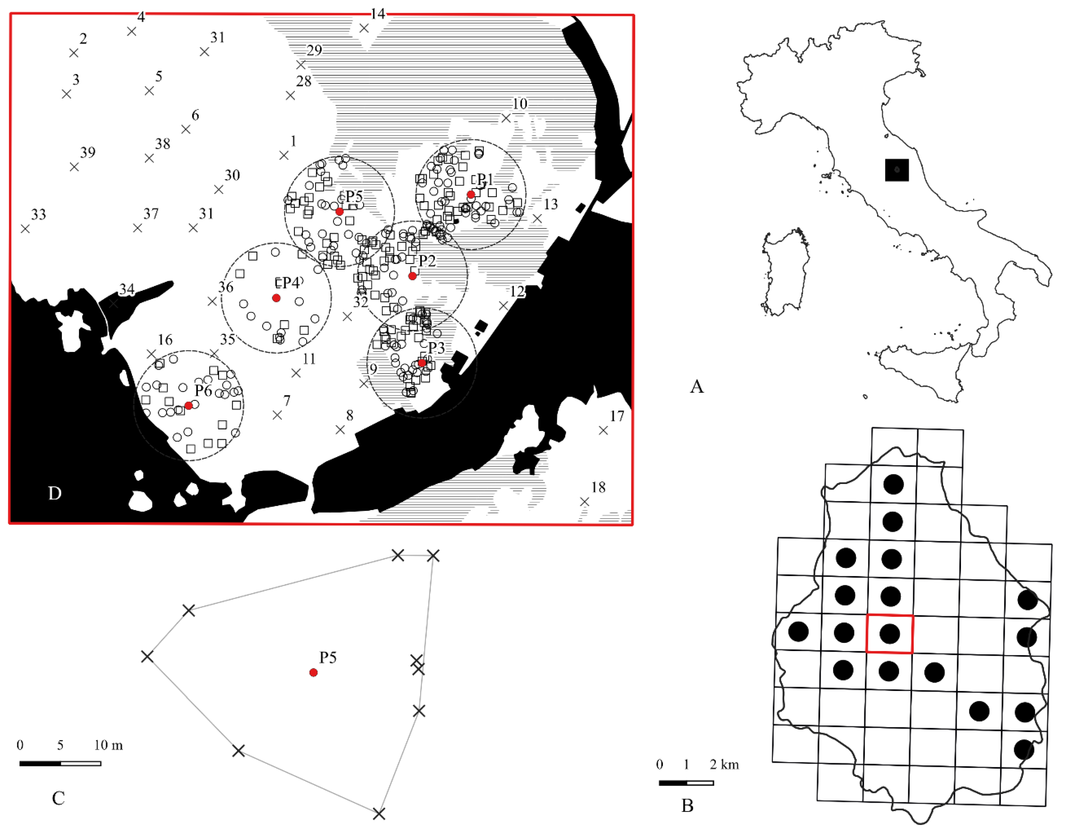
Figure 2.
Left) Insect marking system according to Brussard’s (1971) modification of Earlich and Davidson’s (1960) “1-2-4-7” system described by Southwood (1978). Right) Marking example of the 324th specimen (200+100+20+4 = 324).
Figure 2.
Left) Insect marking system according to Brussard’s (1971) modification of Earlich and Davidson’s (1960) “1-2-4-7” system described by Southwood (1978). Right) Marking example of the 324th specimen (200+100+20+4 = 324).
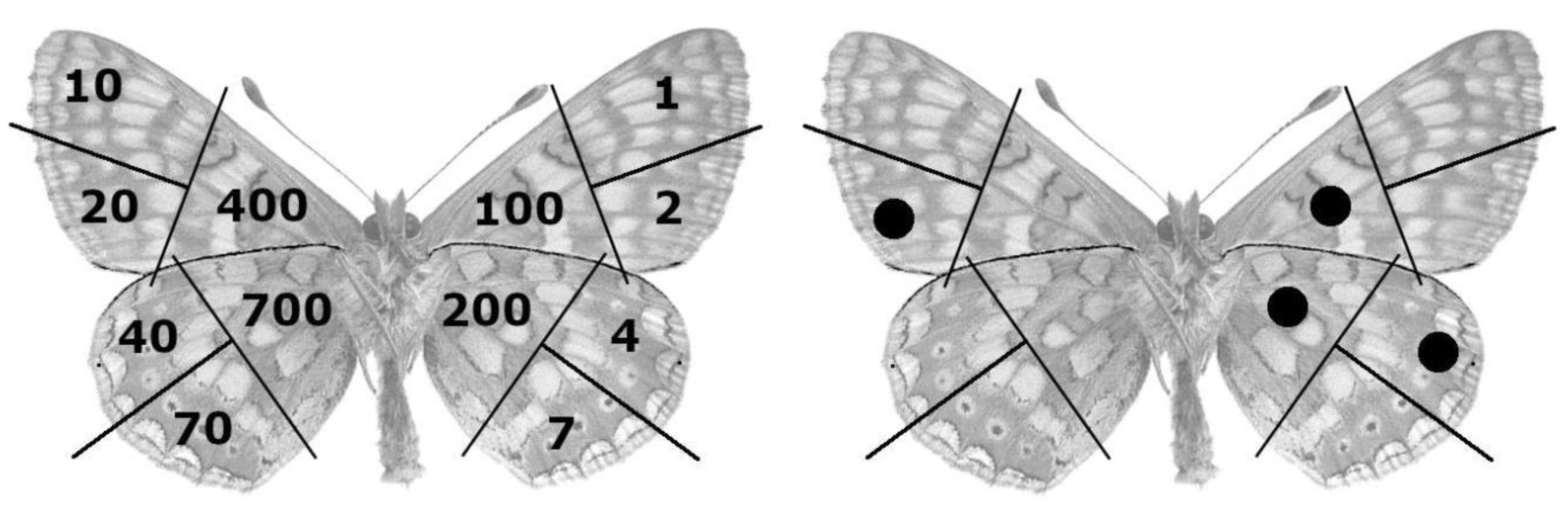
Figure 3.
Bar chart illustrating the percentage composition of plant species used by adults.
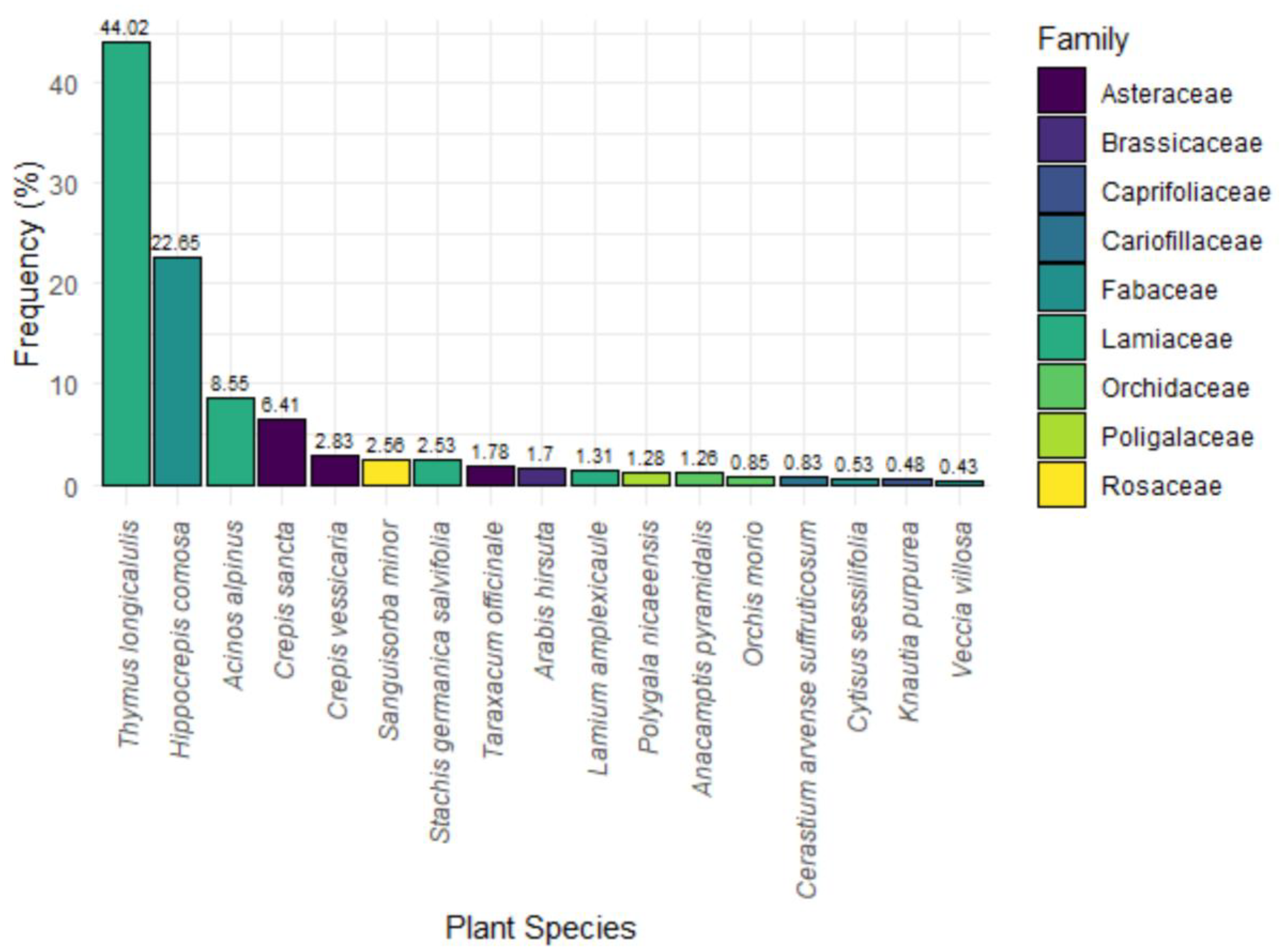
Figure 4.
Distribution frequencies of dispersal distances between sexes.
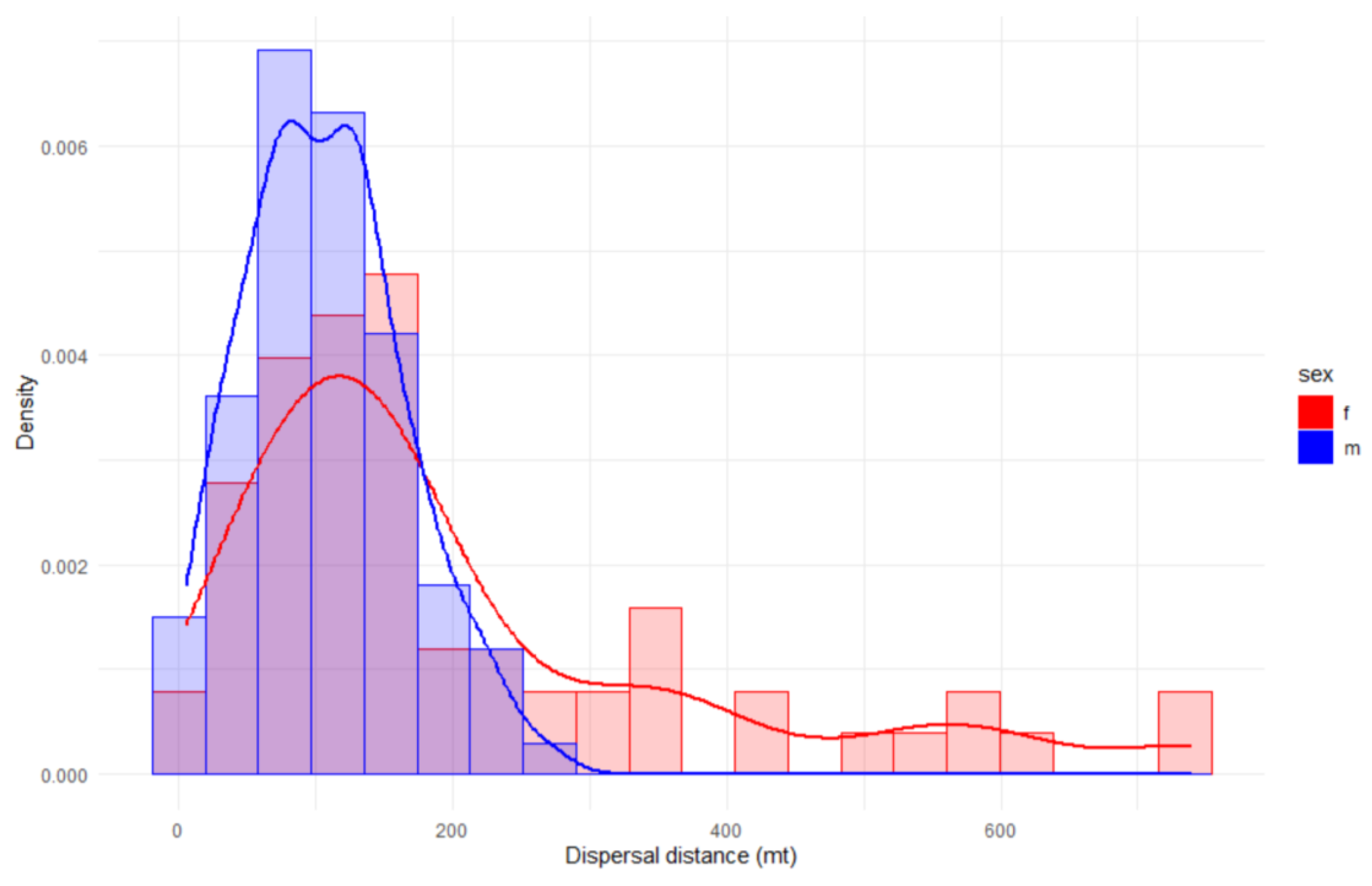
Figure 5.
Relationship between dispersal distance and days since marking for males (blue) and females (red). Points represent individual observations, with LOESS regression lines and confidence intervals. The annotations show Kendall’s p-value (0.965) and the difference in Hoeffding’s D (ΔD = -0.023), indicating a weak but significant time-distance relationship in females, absent in males.
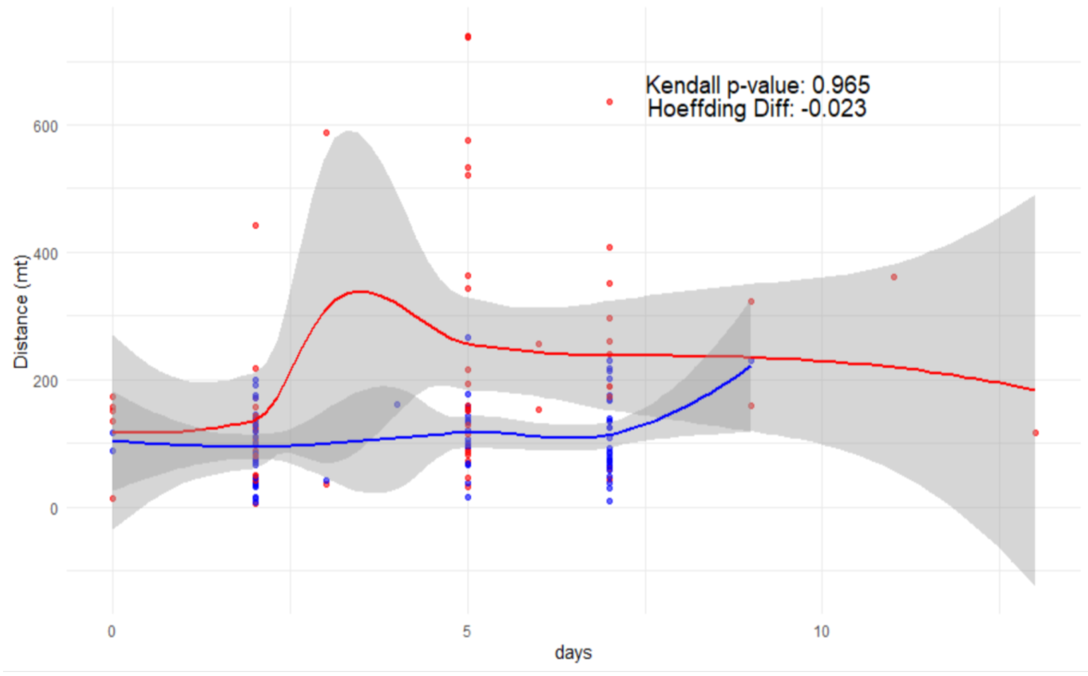
Figure 6.
Relationship between dispersal distance per patch and days since marking for males (blue) and females (red). In females, for patch 5 we have a significative dependence between days and dispersal distance over time.
Figure 6.
Relationship between dispersal distance per patch and days since marking for males (blue) and females (red). In females, for patch 5 we have a significative dependence between days and dispersal distance over time.
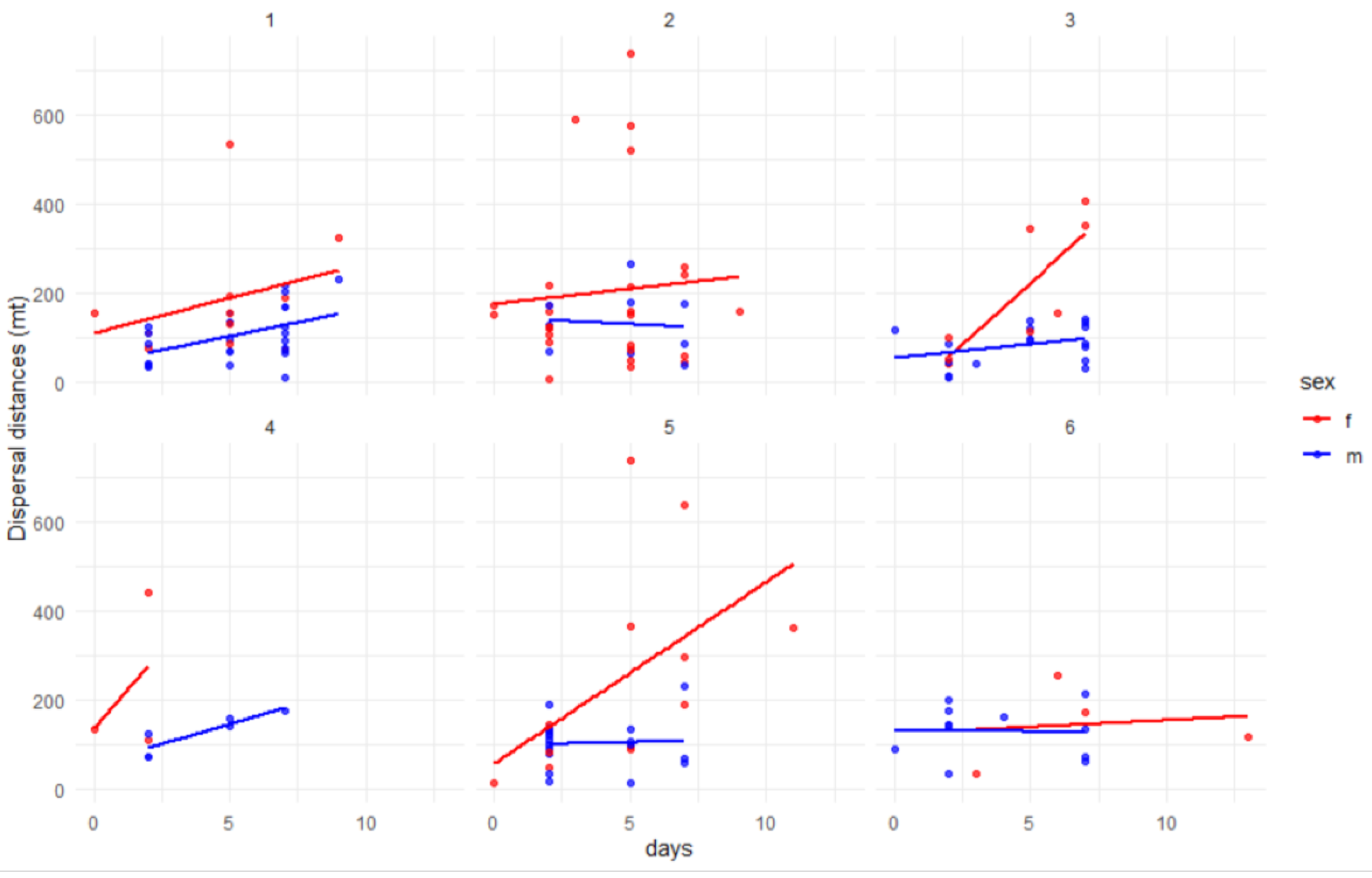
Figure 7.
Patch connectivity network; the size of the node is related to the number of connections the node has with other patches (degree values). The arrows indicate the direction of movement; if there are many arrows starting from a patch it means that it is a source of dispersion (source).
Figure 7.
Patch connectivity network; the size of the node is related to the number of connections the node has with other patches (degree values). The arrows indicate the direction of movement; if there are many arrows starting from a patch it means that it is a source of dispersion (source).
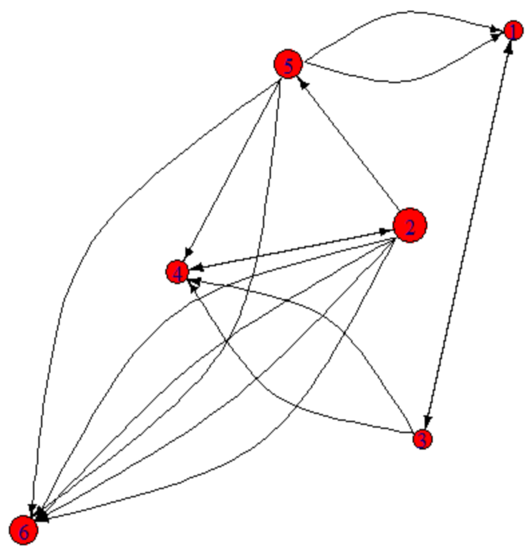
Figure 8.
PCA biplot illustrating the distribution of patches along PC1 and PC2, highlighting the ecological distinction between source (2, 3, 5) and sink patches (1, 4, 6).
Figure 8.
PCA biplot illustrating the distribution of patches along PC1 and PC2, highlighting the ecological distinction between source (2, 3, 5) and sink patches (1, 4, 6).
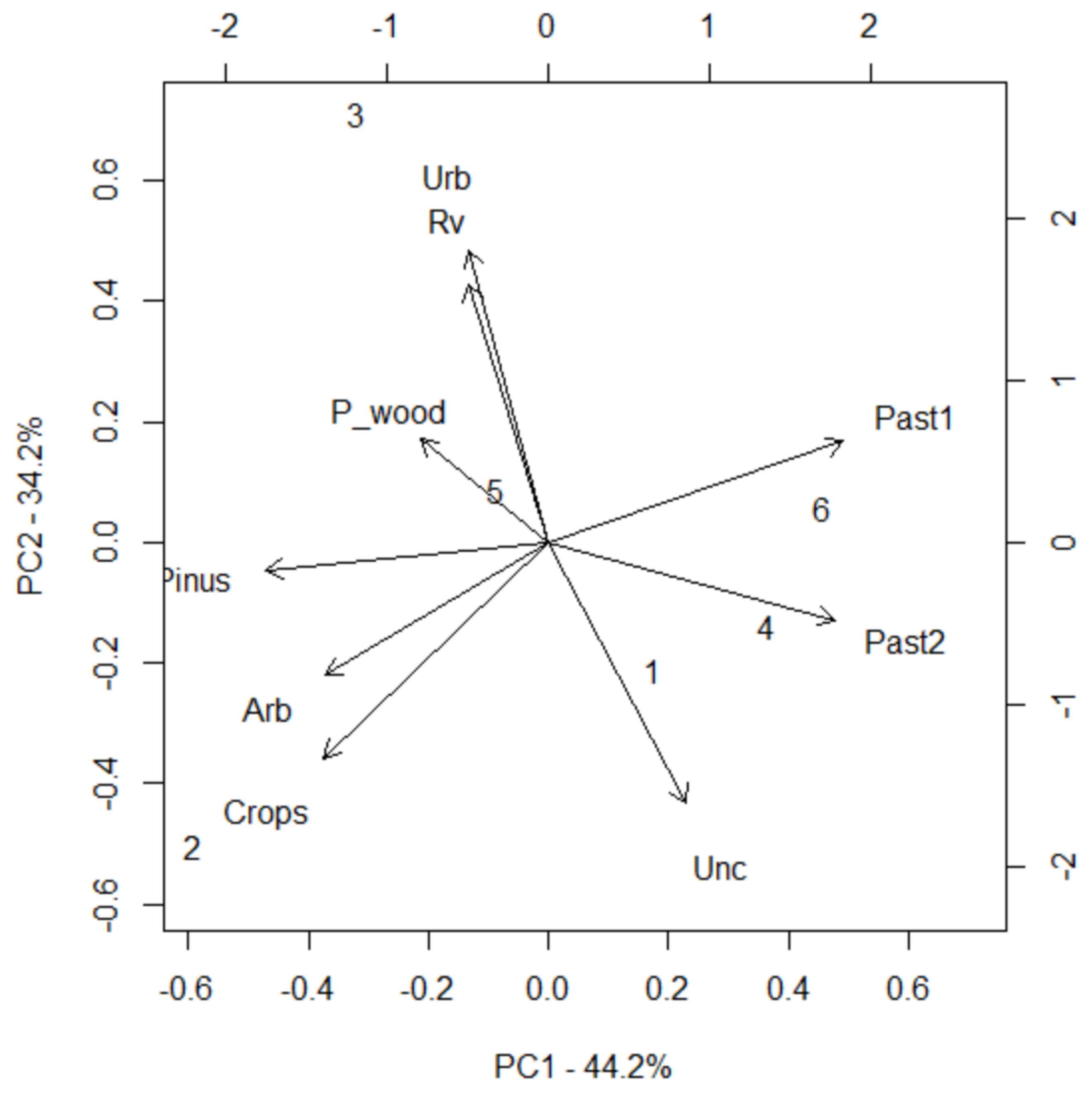

Table 1.
Summary of study area land cover.
| Landcover | COD | Mesh_grid (ha) | Fgrid% | MMRA#break#(ha) | FMMRA% | Fp% |
|---|---|---|---|---|---|---|
| Shrubland | Arb | 7.1 | 3.0 | 1.9 | 4.7 | 26.8 |
| Cropland | Crops | 29.3 | 12.4 | 4,2 | 10.4 | 14.3 |
| Closed-turf grassland | Past1 | 43.4 | 18.4 | 18.2 | 44.9 | 41.9 |
| Open-turf grassland | Past2 | 35.6 | 15.1 | 1.9 | 4.7 | 5.3 |
| Chamaephytic grassland | Past3 | 5.4 | 2.3 | - | - | - |
| Pinus nigra reforestation | Pinus | 27.7 | 11.8 | 3.9 | 9.6 | 14.1 |
| Pre_wood vegetation | P_wood | 12.3 | 5.2 | 3.2 | 7.9 | 26.0 |
| Ruderal vegetation | Rv | 1.3 | 0.6 | 0.2 | 0.5 | 15.4 |
| Uncultivated land | Unc | 13.9 | 5.9 | 5.3 | 13.1 | 38.1 |
| Wet and humid meadows | Wetgrass | 2.6 | 1.1 | 0.4 | 1.0 | 15.4 |
| P.australis community | Pal_ph | 11.6 | 4.9 | - | - | - |
| S.lacustris community | Scirpo | 4.4 | 1.9 | 0.1 | 0.2 | 2.3 |
| Lake and hydrophytic vegetation | Lake | 7.1 | 3.0 | - | - | - |
| Salix alba copses | Salix | 0.5 | 0.2 | - | - | - |
| Urban | Urban | 33.3 | 14.1 | 1.2 | 3.0 | 3.6 |
| 235.5 | 40.5 | 17.2 |
Legend: Arb—Shrubland with a dominance of Cytisophyllum sessilifolium and/or Spartium junceum on the slopes, and of Rhamnus cathartica, Prunus spinosa, Crataegus monogyna, and Rubus sp. pl., in the low-lying areas; Cropland—Arable lands with cereal and legume crops, in rotation with forage crops; Past1—Closed-turf grassland with a dominance of Bromopsis erecta and Brachypodium rupestre, in the slopes with moderately deep soil; Past2—Open-turf grassland with a dominance of Bromopsis erecta, in the slopes with shallow soil; Past3—Open-turf chamaephytic grassland with a dominance of Artemisia alba and Helichrysum italicum, on moderately to very steep slopes with shallow soil, debris, and outcropping rock; Pinus—Pinus nigra reforestation. Pre_wood—Pre-wooded community with Quercus cerris and Acer campestre; RV—Vegetation characterized by nitrophylous and ruderal species, such as Urtica dioica, Sambucus ebulus, Rumex crispus, and Conium maculatum; Unc—Uncultivated land. Salix—Salix alba copses; Pal_ph—Phragmites australis-dominated community in the Colfiorito marsh; Scirpo—Schoenoplectus lacustris-dominated community in the Colfiorito marsh; Lake—Water body with hydrophytic vegetation in the deepest areas of the Colfiorito marsh, characterized by Nymphaea alba and Myriophyllum sp. Pl; Wetgrass—Wet and humid meadows in the low-lying areas at the border of the Colfiorito marsh, characterized by Ranunculus velutinus and sedges (Carex sp. pl.).
Table 2.
Summary of the capture effort, marking and recapture.
| Patch | Lat | Long | number of nests |
number of larvae | Individual marked |
Individual recaptured |
F% |
|---|---|---|---|---|---|---|---|
| 1 | 12.88950 | 43.03211 | 7 | 54 | 634 | 38 | 6.0 |
| 2 | 12.88755 | 43.03011 | 5 | 18 | 486 | 29 | 6.0 |
| 3 | 12.88788 | 43.02798 | 8 | 45 | 483 | 23 | 4.8 |
| 4 | 12.88300 | 43.02957 | 8 | 38 | 483 | 12 | 2.5 |
| 5 | 12.88511 | 43.03169 | 9 | 30 | 731 | 28 | 3.8 |
| 6 | 12.88008 | 43.02692 | 9 | 28 | 436 | 21 | 4.8 |
| Total | 46 | 3253 | 151 | 4.6 | |||
| Mean | 7.7 | 542.2 | 25.2 | ||||
| DS | 1.5 | 114.5 | 8.8 |
Table 3.
Summary of the dispersal distances. SD = Standard Deviation; CV = coefficient of variation calculated as the interval between the first and third quartiles.
Table 3.
Summary of the dispersal distances. SD = Standard Deviation; CV = coefficient of variation calculated as the interval between the first and third quartiles.
| sex | N | Min | Max | Mean | SD | CV |
|---|---|---|---|---|---|---|
| female | 60 | 5.4 | 740.0 | 204.7 | 176.6 | 89.1–256.7 |
| male | 91 | 8.0 | 265.9 | 107.5 | 57.1 | 68.6–138.9 |
| Total | 151 | 5.4 | 740.0 | 149.3 | 132.3 | 73.2–171.7 |
Table 4.
Dispersion balance for each patch with dispersion percentage (DP%).
| Patch | Emigrans | Immigrans | Balance | DP% |
|---|---|---|---|---|
| 1 | 1 | 3 | -2 | 25.0 |
| 2 | 6 | 1 | 5 | 85.7 |
| 3 | 3 | 1 | 2 | 75.0 |
| 4 | 1 | 4 | -3 | 20.0 |
| 5 | 5 | 1 | 4 | 83.3 |
| 6 | 0 | 6 | -6 | 0.0 |
Table 5.
Patch Connectivity Degree with the three Centrality Measures.
| Patch | Degree (connections) |
Betweenness (Bridging role) |
Closeness (Proximity to other patches) | |
|---|---|---|---|---|
| 1 | 4 | 3 | 0.071 | Least proximity |
| 2 | 7 | 8 | 0.125 | High proximity |
| 3 | 4 | 4 | 0.100 | |
| 4 | 5 | 7 | 0.083 | |
| 5 | 6 | 4 | 0.143 | Highest proximity |
| 6 | 6 | 0 | NaN | Disconnected |
Table 6.
Spatial autocorrelation and connectivity analysis results.
| Test | Statistic value |
Expectation | Variance | p-value | Interpretation |
|---|---|---|---|---|---|
| Moran’s I | -0.068 | -0.200 | 0.048 | 0.275 | No spatial autocorrelation |
| Mantel test (r) | 0.015 | - | - | 0.417 | No significant correlation |
Table 7.
Results of the factorial analysis. PC I is the gradient from open to close landscapes factor, while the second indicates a gradient of anthropogenic influence.
Table 7.
Results of the factorial analysis. PC I is the gradient from open to close landscapes factor, while the second indicates a gradient of anthropogenic influence.
| Character | Correlation matrix | |||||
|---|---|---|---|---|---|---|
| PC I (44.2%) | PC II (34.2%) | PC III (14.5%) | ||||
| Eigenvector | Correlation coefficient | Eigenvector | Correlation coefficient | Eigenvector | Correlation coefficient | |
| Arb | -0.35427 | -0.70647 | -0.23640 | -0.41495 | -0.36498 | -0.41773 |
| Crops | -0.35747 | -0.71284 | -0.38600 | -0.67755 | 0.00609 | 0.00697 |
| Rv | -0.12817 | -0.25558 | 0.46354 | 0.81366 | -0.36459 | -0.41728 |
| P_wood | -0.20349 | -0.40579 | 0.18517 | 0.32504 | 0.73730 | 0.84385 |
| Past1 | 0.46637 | 0.93000 | 0.18092 | 0.31758 | -0.06923 | -0.07923 |
| Past2 | 0.45387 | 0.90508 | -0.13993 | -0.24562 | -0.23405 | -0.26787 |
| Pinus | -0.44912 | -0.89560 | -0.04950 | -0.08689 | -0.23589 | -0.26998 |
| Unc | 0.21849 | 0.43570 | -0.46460 | -0.81552 | -0.10585 | -0.12115 |
| Urb | -0.12621 | -0.25168 | 0.52473 | 0.92106 | -0.25258 | -0.28908 |
Legend: Arb—Shrubland with a dominance of Cytisophyllum sessilifolium and/or Spartium junceum on the slopes, and of Rhamnus cathartica, Prunus spinosa, Crataegus monogyna, and Rubus sp. pl., in the low-lying areas; Cropland—Arable lands with cereal and legume crops, in rotation with forage crops; Past1—Closed-turf grassland with a dominance of Bromopsis erecta and Brachypodium rupestre, in the slopes with moderately deep soil; Past2—Open-turf grassland with a dominance of Bromopsis erecta, in the slopes with shallow soil; Pinus—Pinus nigra reforestation. Pre_wood—Pre-wooded community with Quercus cerris and Acer campestre; RV—Vegetation characterized by nitrophylous and ruderal species, such as Urtica dioica, Sambucus ebulus, Rumex crispus, and Conium maculatum; Unc—Uncultivated land. PC I, II, III = Principal component I, II, III.
Table 8.
Results of the Welch Two Sample t-test comparing PCA scores (PC1 and PC2) between source and sink patches. Mean scores values are presented with standard deviation (Mean ± SD).
Table 8.
Results of the Welch Two Sample t-test comparing PCA scores (PC1 and PC2) between source and sink patches. Mean scores values are presented with standard deviation (Mean ± SD).
| Principal Component | Statistic value |
Mean ± SD (source) |
Mean ± SD (sink) |
t-value | df | p-value |
|---|---|---|---|---|---|---|
| PC 1 | -0.068 | -1.23 ± 0.56 | 1.45 ± 0.72 | 2.94 | 4.87 | 0.025 |
| PC 2 | 0.015 | 0.38 ± 0.47 | 0.29 ± 0.51 | 0.50 | 5.14 | 0.636 |
Disclaimer/Publisher’s Note: The statements, opinions and data contained in all publications are solely those of the individual author(s) and contributor(s) and not of MDPI and/or the editor(s). MDPI and/or the editor(s) disclaim responsibility for any injury to people or property resulting from any ideas, methods, instructions or products referred to in the content. |
© 2025 by the authors. Licensee MDPI, Basel, Switzerland. This article is an open access article distributed under the terms and conditions of the Creative Commons Attribution (CC BY) license (http://creativecommons.org/licenses/by/4.0/).
Copyright: This open access article is published under a Creative Commons CC BY 4.0 license, which permit the free download, distribution, and reuse, provided that the author and preprint are cited in any reuse.


