
Submitted:
18 June 2025
Posted:
20 June 2025
You are already at the latest version
Abstract
Understanding how training and match load influence autonomic recovery is essential for optimizing athlete monitoring. This study aimed to examine the impact of training and match load on next-day heart rate variability (HRV) and to identify the most influential predictors by applying SHapley Additive Explanations (SHAP) to interpret machine learning models. Five semi-professional basketball players (23 ± 5 years; 191 ± 7 cm; 90 ± 11 kg) were monitored throughout a competitive season. HRV and load metrics were recorded daily. Differences in the natural logarithm of the root mean square of successive differences (LnRMSSD) across Non-Training, Training, and Match days were analyzed using linear mixed models. Additionally, a Gradient Boosting Machine model was developed to predict next-day HRV responses, with SHAP analysis providing both global and individual insights into feature importance. Next-morning LnRMSSD values were significantly lower on Match days compared to both Training and Non-Training days (p < 0.001). SHAP results identified rate of perceived exertion (RPE), days since last match, minutes played, and recent training load as the most influential predictors of HRV changes. Pre-session heart rate and the root mean square of successive differences (RMSSD) values also demonstrated notable individual relevance. The ranking and magnitude of influential variables varied across players, highlighting the heterogeneity of physiological responses in team sports. These findings underscore the importance of integrating both subjective and objective load measures when managing training in basketball. SHAP improves the interpretability of predictive models and supports the implementation of individualized monitoring strategies to optimize recovery and performance throughout the microcycle.
Keywords:
machine learning
; SHAP analysis
; heart rate variability
; load monitoring
; basketball
1. Introduction
In team sports, where the competitive period spans several months, a well-structured approach to load quantification is essential [1,2]. During a competitive microcycle, sport scientists must monitor load and recovery to promote adaptation, minimize fatigue, and reduce injury risk in team-sports athletes [1,3]. Training load can be categorized into external and internal components, with external load referring to the work performed by the athlete during training or competition, and internal load referring primarily to the physiological response [2,4,5]. Basketball involves intermittent high-intensity actions and diverse player profiles across positions, each with distinct physical and tactical demands [6,7,8]. Combined with a congested schedule, this underscores the need for individual monitoring of internal and external load. A common method for load monitoring is heart rate (HR)-based measurements [9,10]. Metrics derived from HR monitoring, such as heart rate variability (HRV), can provide insights into the status of the autonomic nervous system and its potential relationship with fatigue [9,10]. HRV, sensitive to the prior day’s stimulus [4,11,12,13], can support assessment of physiological response and optimize the dose-response process throughout the competitive microcycle in basketball players.
HRV refers to the fluctuation in the time intervals between consecutive heartbeats [14]. It responds differently to high- and low-intensity stimuli [15], and exhibits individual variation [12,16,17], highlighting the need for individualized monitoring and analysis for each athlete. Among various HRV metrics, the Root Mean Square of Successive Differences (RMSSD) and its logarithmic transformation (LnRMSSD) have been widely used for fatigue monitoring in team sports [11,12,16,18,19]. However, individual responses to load must be considered, and individual LnRMSSD values have been used to observe training responses, highlighting the athlete heterogeneity in team sports [12,18]. HRV-based load modulation usually involves adjusting training based on the morning HRV reading [13], but this is often limited by time constraints in team settings. Therefore, predictive models of HRV responses to training loads could improve planning and decision-making during the competitive microcycle. Additionally, given the length of the competition period in team sports, considering HRV trends and load evolution across the entire season is also important. However, most studies have focused on partial periods such as pre-seasons or short cycles [11,17,18,20]. Likewise, there does not appear to be a clear consensus in the literature regarding the relationship between HRV and other load-related variables, as this relationship tends to be highly individual and vary depending on the monitoring method used [11,18,19,21,22]. Consequently, more research on predictive models is needed to better characterize these complex relationships and enhance proactive load management in basketball players.
In this context, advanced methods such as the SHapley Additive exPlanation (SHAP) technique offer a unique opportunity to improve the explainability of competitive black-box algorithms such as Gradient Boosting Models by identifying the contributing variables and enabling timely and informed adjustments [23]. This one can be used to relate a response variable, such as LnRMSSD with load variables that mostly influence on athlete’s fatigue reflected in HRV changes. SHAP technique provides values (SHAP values), which would allow to know the contribution (positive or negative) of each load variable to the LnRMSSD prediction given by the model for each athlete and, globally, the importance and contribution of each variable load in the model. This is particularly valuable in team sports, where the interaction of multiple complex variables can complicate data-driven decision-making.
Therefore, the aims of this study were: i) To assess the effect of the previous day’s stimulus on HRV; ii) To build a model that explains which load variables affect HRV in basketball players, based on monitoring them throughout an entire season.; iii) To identify individual profiles regarding the specific factors that influence HRV changes. We hypothesized that the training or match load from the previous day could influence the HRV response on the following day, and that specific load variables would explain this modification to a greater extent. Additionally, we expected to find individual differences among athletes in the factors influencing these responses.
2. Materials and Methods
2.1. Study Design
A longitudinal observational study with a repeated measures design was conducted, recording training load variables, rate of perceived exertion (RPE), training and match volume and HRV throughout a semi-professional basketball season in Spain (2021-2022). Daily recordings were performed, and only players who completed the full monitoring were included in the statistical analysis. Data were collected over a period of seven months (October to April) by the strength and conditioning coach as part of their professional development.
2.2. Participants
Five semi-professional basketball players (age: 23±5 years; height: 191 ± 7 cm; body mass: 90 ±11 kg) voluntarily participated in this study. Based on playing positions, they were grouped as: 2 point guards, 2 wings, and 1 center. Each player contributed an average of 212.6 ± 23.9 HR and HRV recordings and 257 RPE and volume recordings. The typical weekly schedule during the season included four training sessions and one match. On average, each player had 98 ± 9.77 training session recordings and 26.6 ± 2.19 match recordings. All participants were fully informed about the study procedures and gave their consent for the use of their data. Additionally, written informed consent was obtained from the club to analyze the data collected throughout the season. As data used in this study were collected as part of routine player monitoring, no ethics committee approval was required [24].
2.3. Procedures
2.3.1. Training Days Classification (MD-TD-NTD)
During the season, days were classified into three categories based on their content: match day (MD), training day (TD), or non-training day (NTD). A match day was defined as any day the player participated in at least one minute of an official game. A training day was recorded when there was a team training session in which the player participated fully. A non-training day was recorded when the player did not participate in either a game or training session that day. The typical in-season microcycle was structured as shown in Figure 1.
2.3.2. Training Load
The primary load metrics recorded were training session duration or match minutes played, and subjective effort assessment via RPE. From these two metrics, session-RPE (sRPE) was calculated by multiplying volume and RPE. RPE is a valid tool for recording training load[25]. All metrics used can be found in Table A1. RPE data were collected using the TrainingFeel app (https://trainingfeel.com/), which enables automated reporteing of Borg’s 1-10 scale by each player on their own mobile device. Data collection was preceded by a two-week familiarization phase and conducted individually. Each player answered the question “How intense did the session feel?” on their mobile device 15-30 minutes post-session. Session duration for each player was monitored by the team’s strength and conditioning coach, while match minutes were obtained from the official records on the Spanish Basketball Federation’s website (https://www.feb.es/).
For each of these variables, the moving average, weighted average, and exponentially weighted moving average (EWMA) were calculated[26]. A more detailed explanation of the EWMA can be found in Table A1. The average was calculated as the mean of the last few days, with the number of days included indicated in the variable name (e.g., sRPE_avg4). The weighted average was calculated by weighting the same average, giving a higher value to the most recent day (4 in the case of a four-day period) and reducing by one for each preceding day. The EWMA was calculated using the formula previously applied in other studies on load monitoring in sports [27].
2.3.3. Heart Rate Variability
To monitor load responses, HR data were collected during training sessions and matches [10]. From these, HR, RMSSD, and LnRMSSD were derived. HRV monitoring, particularly through LnRMSSD, has been used by various authors as a method to assess the response to training load [9,16].
For HR data collection, participants downloaded the validated HRV4Training app [28] (http://www.hrv4training.com/) and consented to data recording and processing for professional development and research purposes via the app itself. Each morning, upon waking, HRV was measured in a one-minute supine recording to avoid external stressors [29]. A measurement was considered valid if confirmed by the app’s algorithm. Ultrashort recordings have shown validity and are sensitive to the prior day’s stimulus [30]. The measurement was conducted using the photoplethysmography (PPG) method. PPG was used as a non-invasive and validated method to assess autonomic nervous system status[30], with participants placing their finger over the mobile device’s camera and flash. Data were uploaded automatically to a cloud server and accessed by the strength and conditioning coach.
2.4. Statistical Analyses
Descriptive data are presented as mean ± standard deviation. Firstly, the linear mixed-effects model analysis was conducted to examine the effects of different types of days (MD, TD or NTD) on HRV, specifically LnRMSSD. The day category was set as a fixed effect factor, whereas the intercept was allowed to vary randomly across participants to account for individual differences in LnRMSSD for the reference condition (i.e., NTD). Post-hoc contrast were performed by paired t-tests with Bonferroni’s correction. Normality of the residuals was visually inspected (i.e. histogram and Q-Q plots) whereas kurtosis and skewness statistics were also considered.
On the other hand, we aimed to adjust a model that allowed establishing the dependency relationships between the LnRMSSD variable and load indicators of basketball players. Although there are quite popular and interpretable techniques such as decision trees and regression models, the fact that the relationships involved in the current study can be especially complex led us to opt for more sophisticated models. Among them, we used an Extreme Gradient Boosting (XGBoost), which consists of the sequential adjustment of hundreds of decision trees, where each one assigns greater weight to the patterns worst predicted by the previous trees. This is why it is considered as a black-box type model, whose results are competitive, from a predictive point of view. In this context, the SHAP technique is applied to quantify the contribution of each variable in the model (i.e., load variables; see Table A1) to the predicted outcome (LnRMSSD) through the computation of SHAP values. Furthermore, this interpretation can be done both at a global level, to identify the most relevant variables to characterize the LnRMSSD, and at a local level, that is, at the athlete level. The latter is decisive to be able to make personalized decisions about each of them. Thus, one variable may be the one that generally contributes the most to an increase or decrease in the LnRMSSD, and yet another variable may be the one that is most relevant for a specific athlete. In this study normal level of LnRMSSD was defined as the average of NTD ± 0.5 SD within the last 30 days and therefore being updated daily.
LnRMSSD was estimated using an Extreme Gradient Boosting Model. Regarding the model configuration, hyperparameters were tuned using grid search five-fold cross-validation minimizing the root mean squared error (RMSE). The final model included 400 trees, a learning rate of 0.01, a maximum depth of 4 and a subsample of 0.6 as hyperparameters. To obtain explanations of the features that drive players-dates estimates, we used a SHAP algorithm. SHAP plots provided a clear and intuitive way to visualize the contributions of various features to our model’s estimates, proving to be an invaluable tool in understanding the factors that underline predictions related to LnRMSSD. The application of SHAP plots allowed us to analyze the impact of individual features on LnRMSSD estimates, encompassing both the direction and magnitude of their influence. In these plots, the magnitude of the value of the load variables is represented by colors, while the influence over the predicted given by the model is expressed by a Shapley value. In fact, these values represent the contribution (positive or negative) of each load variable to the LnRMSSD prediction given by the model.
By closely examining SHAP values, this analytical approach facilitated the identification of the input variables in the estimate of LnRMSSD. Thus, once a variable and an observation have been fixed, it will be represented by a dot. This dot will be associated with a more intense red color, the higher the value of the variable on that observation, and a more intense blue color the lower the value. In addition, the higher the Shapley value (i.e., the farther to the right the observation is represented), the greater the contribution of the variable to the increase in the estimate given by the model for that observation. Conversely, the lower the Shapley value (i.e., the further to the left the observation is represented), the greater the contribution of the variable to the decrease in the estimate given by the model for that observation. In consequence, the sign informs whether the variable contributes positively or negatively to the estimate made for the observation. According to their global influence on the model, the variables will be presented from greater to lesser importance on the Y axis.
On the other hand, linear mixed model analysis was carried out using SPSS software v.28 (IBM Corp., Armonk, NY, USA), with a significance level set at p < 0.05, whereas the explanatory framework model was performed using the Python package XGBoost in Python 3.11.3 (Python Software Foundation, Oregon, USA)
3. Results
Values of LnRMSSD were analyzed according to the categorization of days using mixed models. The estimated marginal means for each type of day were: 4.711 ± 0.146 ln (ms) for NTD, 4.653 ± 0.146 ln (ms) for TD, and 4.408 ± 0.149 ln (ms) for MD.
Pairwise comparisons (Figure 2) revealed significant differences between NTD and MD ( mean difference = 0.304, p < 0.001) and between TD and MD (mean difference = 0.245, p < 0.001), whereas non-significant differences were observed between NTD and TD (mean difference = 0.058, p = 0.578).
The SHAP analysis shows the contribution of different variables to the modification of LnRMSSD (Figure 3). The most impactful variables include RPE, the number of days since the last match (DaysLastMatch), minutes played in the last match (Volume_LastMatch), the average sRPE of the last four days, and the RPE of the last match (RPE_LastMatch), among others. Additionally, variables such as pre-training or pre-match RMSSD and HR also influence the modification of LnRMSSD on the following day.
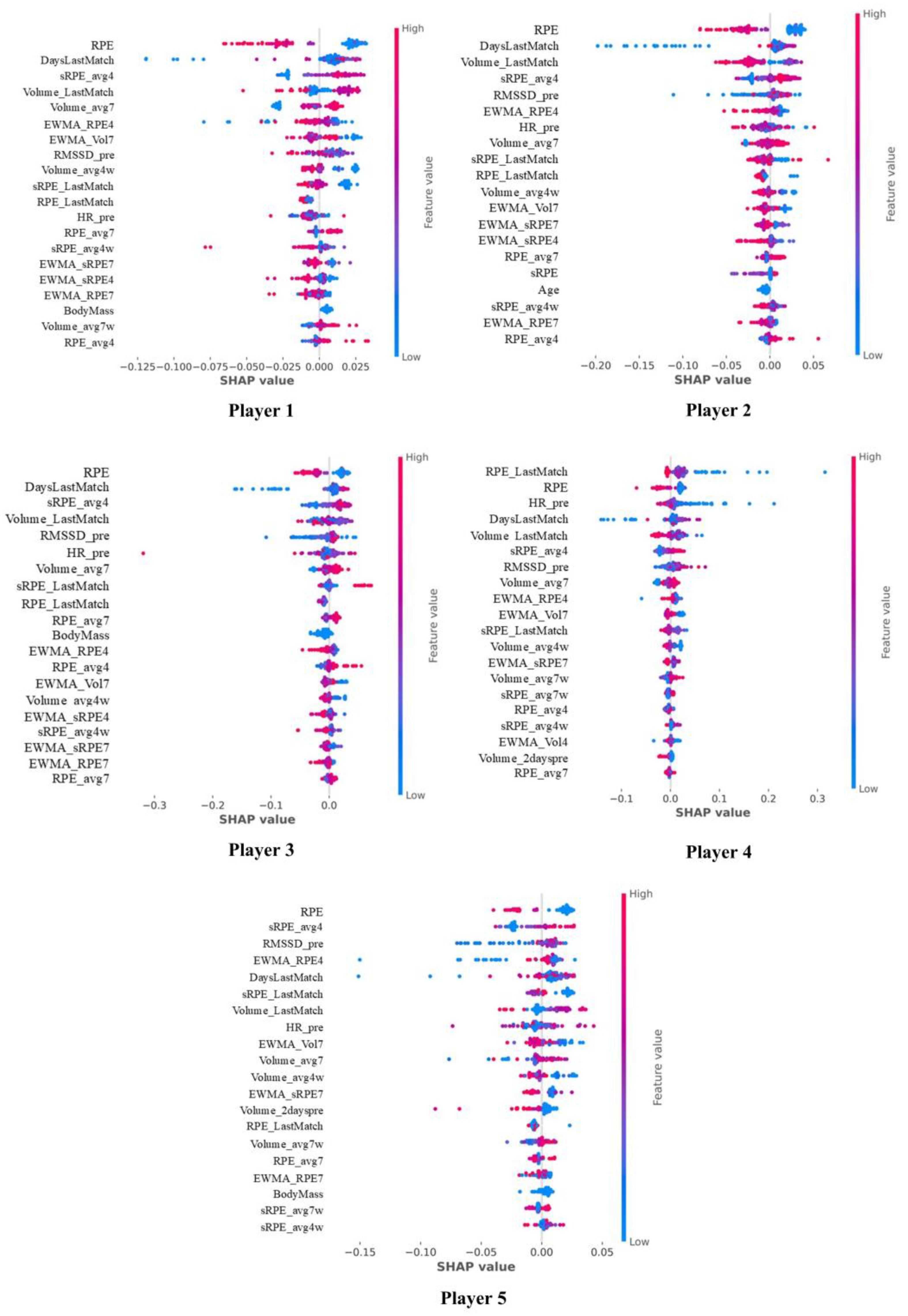
Figure 4 displays the individual analyses, highlighting inter-individual differences in the order, weight, and impact of the variables associated with HRV changes for each player.
4. Discussion
The main findings of this study are: i) HRV is influenced by the training load from the previous day, with matches being the stimulus that induces the greatest change; ii) intensity metrics appear to be one of the most important variables explaining HRV variation on the following day; iii) individual differences exist regarding which variables most influence HRV modification in each player.
Previous research has shown that HRV is influenced by training load in team-sport athletes[12,19]. Consistent with these findings, our results indicate that LnRMSSD is affected by training load in semiprofessional basketball players. However, those studies focused on short-term periods [11,12,18] such as a single competitive microcycle or preaseason. In contrast, the present study monitored players across a full competitive season. Specifically, our results show a significant difference between MD and both TD and NTD, while no differences were found between TD and NTD. This may be due to the variability of training sessions, which ranged from low to high intensity. Nakamura et al. [31] reported a decrease in LnRMSSD the morning following matches during a beach volleyball tournament, though they did not compare this response to training sessions, leaving uncertainty about HRV responses to different stimuli. Our findings appear to support structuring the microcycle around the match and its proximity, as the match appears to elicit the largest suppression of LnRMSSD. One of the limitations of previous studies is the lack of direct comparisons between physiological responses to matches and training. Future research should address this to determine whether matches consistently cause greater HRV reductions and to clarify the implications of this response.
Through SHAP analysis, RPE and days since the last match were identified as the two most influential variables in HRV changes. Consistent with previous research [15,30], perceived intensity through RPE appears to be the main factor influencing HRV [32]. In a previous study, O’Connor et al. [19] reported a relationship between sprint volume and a reduction in RMSSD upon waking the following day. Similarly, Stanley et al. [15], found that while HRV tends to recover within 24 hours following low-intensity exercise, high-intensity sessions suppress HRV for up to 48 hours post-exercise. Our findings, highlighting RPE as the main variable, align with these authors, reinforcing the impact of exercise intensity on next-day HRV suppression. The number of days since the last match ranks second, suggesting that having a match the previous day negatively affects HRV, which highlights the importance of organizing the days following the match due to their high-intensity nature, and the need for at least 48 hours for full parasympathetic cardiac reactivation [15]. These findings suggest that match intensity and recovery window should be key considerations in basketball microcycle planning. Minutes played in the match also significantly influenced HRV, with higher values of minutes played linked to decreased LnRMSSD the following day. We also identified a third key metric related to the match: the reported RPE metric that refers to the RPE reported in the last match played. Therefore, these results seem to highlight the importance of the match in HRV response, along with minutes played and match RPE as a key metrics for predicting players’ HRV responses. Since HRV can also be influenced by psychological variables[33], match demands and outcomes may play a role in the magnitude of these changes. The average sRPE of the last 4 days showed an inverse relationship with the next-day LnRMSSD. Since it links both volume and perceived intensity metrics, the response may be primarily influenced by the volume, as it takes higher values than RPE. This effect was clearer when analyzing the 7-day average volume, which appeared to positively influence HRV. This suggests that training exposure may help sustain favorable HRV values [21], although acute responses depend on session intensity [15,19]. Pre-stimulus variables such as HR and pre-match RMSSD also play a significant role in the response the following day. Higher resting HR or lower RMSSD values prior to training seem to influence a greater reduction in LnRMSSD the next day. Taken together, these results suggest the need to plan training loads during the microcycle by taking into account not only the match and the intensity of training sessions, but also the athlete’s physiological status prior to each session. Considering the clear impact that match-related variables and perceived intensity have on HRV modulation, practitioners should incorporate these findings into the weekly planning process to optimize the balance between stimulus and recovery and ultimately support performance and adaptation.
Individual differences were observed in the training load metrics associated with HRV responses. Similarly, Flatt et al. [16] reported in American football, differences among players. This highlights the importance of individualizing the monitoring process based on the specific characteristics of each athlete. Each player exhibits a unique profile in which specific metrics have varying degrees of importance and magnitude in HRV modification. Differences are observed between Player 1 (wing) and Player 5 (point guard) regarding the position and effect of the RMSSD_pre variable. For instance, in Player 1, RMSSD_pre ranks eighth in importance for HRV response, while in Player 5, it ranks third. Furthermore, in Player 5, there is a clear tendency where low RMSSD_pre values significantly and negatively influence HRV, whereas in Player 1, the effect is less pronounced, and it appears that high RMSSD_pre values have a negative influence. Differences are also observed in Player 3 (point guard), where the HR_pre metric holds high importance, ranking third. It shows a clear influence, with low values having a positive effect, while high or medium values have little to no effect, or even a negative influence. In the other players, this metric appears with lower importance, and its interpretation is less clear, with mixed influences from both high and low values. These findings suggest that individual profiles should be considered when managing training load and monitoring potential fatigue. The SHAP analysis provides an easy-to-interpret individual and global interpretation, allowing us to translate it into a practical application for coaches and strength and conditioning professionals.
To the best of the authors’ knowledge, this is the first study to apply SHAP analysis to model athlete fatigue, considering different types of variables recorded throughout an entire competitive season. This technique enables the development of both general and individual predictive models, rather than relying on the retrospective decision-making approach provided by other analytical methods. Our results showed that RPE and the number of days since the last match were the most predictive variables of player condition, as assessed through HRV. However, distinct individual profiles were also identified. Machine learning techniques, combined with interpretability methods such as SHAP, emerge as valuable tools for identifying predictive models of fatigue and performance in team sports, allowing for the anticipation of training load adjustments.
There are some limitations in the present study that should be acknowledged. Firstly, the sample size limits the study’s ability to draw broader conclusions, although a substantial amount of data per player was used to train the mathematical model. Secondly, we analyzed only a single season, whereas a larger longitudinal study would be beneficial to confirm the findings. Nevertheless, to our knowledge, this is the first study to use data from an entire competitive season to develop a predictive model of fatigue in team sports. Finally, training load was assessed using RPE, while integrating additional objective measures, such as accelerometers or other sensors, would be valuable for future research. However, RPE and sRPE have been shown to reflect internal load in team sports [8,34].
5. Conclusions
The results of the present study showed that HRV is significantly influenced by the training load from the previous day, with matches being the stimulus that induces the greatest change. RPE and the number of days since the last match, were identified as the main factors affecting LnRMSSD modification. Additionally, playing time in the last match and the physiological state before training or competition (HRV and HR) also influenced HRV responses on the following day. In addition, the individual analyses revealed differences among players regarding the most influential variables and their impact on HRV modification. These findings highlight the importance of considering individual profiles when managing training load and monitoring fatigue status in basketball players.
To the best of the authors’ knowledge, this study is the first to apply SHAP analysis to model athlete fatigue, as measured by HRV, over an entire competitive season in a team sport, enabling the identification of both general and individual response patterns to training load. The integration of machine learning techniques with interpretable methods such as SHAP provides valuable tools for anticipating training load adjustments, optimizing performance, and enhancing recovery in team sports.
Author Contributions
Conceptualization, J.A-L. and E.I-S.; methodology, J.A-L., E.I-S. and A.P-C.; formal analysis, J.A-L, E.I-S.., D.V-S. and A.A-M.; Validation, D.V-S. and A.A-M.; Software, D.V-S. and A.A-M.; investigation, J.A-L., E.I-S.; data curation, J.A-L.; writing—original draft preparation, J.A.L.; writing—review and editing, E.I-S., A.P-C.; visualization, D.V-S. and A.A-M.; supervision, E.I.-S.; project administration, J.A-L. and E.I-S. All authors have read and agreed to the published version of the manuscript.
Funding
This research received no external funding.
Institutional Review Board Statement
Ethical review and approval were waived for this study as the data analyzed were collected through routine player monitoring procedures conducted during the season.
Informed Consent Statement
Informed consent was obtained from all subjects involved in the study.
Data Availability Statement
Data are available upon request from the corresponding author due to privacy and ethical restrictions.
Conflicts of Interest
The authors declare no conflicts of interest.
Abbreviations
The following abbreviations are used in this manuscript:
| EWMA | Exponentially Weighted Moving Average |
| HR | Heart Rate |
| HRV | Heart Rate Variability |
| LnRMSSD | Natural Logarithm of the Root Mean Square of Successive Differences |
| MD | Match Day |
| NTD | Non-Training Day |
| PPG | Photoplethysmograph |
| RMSE | Root Mean Squared Error |
| RMSSD | Root Mean Square of Successive Differences |
| RPE | Rate of Perceived Exertion |
| SHAP | SHapley Additive exPlanation |
| sRPE | Session Rate of Perceived Exertion |
| TD | Training Day |
| XGBoost | Extreme Gradient Boosting |
Appendix A

Table A1.
List of variables included in the SHAP analysis.
| Name | Definition |
|---|---|
| Height | Height in centimeters. |
| Age | Age at the start of the season |
| BodyMass | Body mass in kilograms |
| MD-TD-NTD | Classification of days based on whether it was a match day (MD), training day (TD), or non-training/non-match day (NTD). |
| Volume | Volume in minutes of session duration in the case of training days. For matches, the number of minutes played in the game. |
| Volume_2dayspre | Volume metric (in minutes) from the two days prior to the HRV measurement (as HRV is measured the morning following the stimulus). |
| Volume_avg4 | Mean volume (in minutes) over the last 4 days |
| Volume_avg7 | Mean volume (in minutes) over the last 7 days |
| Volume_avg4w | Weighted average of the volume over the last 4 days, with a weight of 4 for the most recent day, 3 for the following day, 2 for the next, and 1 for the day furthest back. |
| Volume_avg7w | Weighted average of the volume over the last 7 days, with a weight of 7 for the most recent day and decreasing by one each day until assigning a weight of 1 to the day furthest back. |
| Volume_LastMatch | Minutes played in the last match |
| EWMA | Exponentially Weighted Moving Average Method for monitoring load through the acute-to-chronic ratio, which assigns a decreasing weight to each older load value, thereby giving greater weight to recent load. EWMA=Metric × λ+((1- λ) ×(EWMAyesterday)), Where Metric refers to the observed value in the load metric (RPE, Volume, etc.), Lambda represents a constant between 0 and 1 that determines the depth of how many days influence the calculation. Assigning a lower value means that older values retain significant weight for a longer period. EWMA yesterday refers to the EWMA value for the previous day. |
| EWMA_RPE4 | EWMA of the RPE variable where lambda equals 4 |
| EWMA_RPE7 | EWMA of the RPE variable where lambda equals 7 |
| EWMA_sRPE4 | EWMA of the sRPE variable where lambda equals 4 |
| EWMA_sRPE7 | EWMA of the sRPE variable where lambda equals 7 |
| EWMA_Vol4 | EWMA of the Volume variable where lambda equals 4 |
| EWMA_Vol7 | EWMA of the Volume variable where lambda equals 7 |
| HR | Heart rate (in beats per minute) on the day following to the stimulus. |
| HR_pre | Early morning heart rate (in beats per minute) on the same day as the training or match. |
| RMSSD | Calculating each successive time difference between heartbeats in milliseconds. Then, each of the values is squared and the result is averaged before the square root of the total is obtained. |
| RMSSD_pre | Early morning RMSSD in milliseconds on the same day as the training or match. |
| LnRMSSD | A natural log is applied to the RMSSD to smooth the data and facilitate interpretation. |
| RPE | Subjective rating of session intensity was assessed using Borg’s 1-10 scale, in response to the question, ‘How intense did the session feel?’ |
| RPE_2days | RPE metric from the two days prior to the HRV measurement (as HRV is measured the morning following the stimulus). |
| RPE_avg4 | Mean RPE over the last 4 days |
| RPE_avg7 | Mean RPE over the last 7 days |
| RPE_avg4w | Weighted average of the RPE over the last 4 days, with a weight of 4 for the most recent day, 3 for the following day, 2 for the next, and 1 for the day furthest back. |
| RPE_avg7w | Weighted average of the RPE over the last 7 days, with a weight of 7 for the most recent day and decreasing by one each day until assigning a weight of 1 to the day furthest back. |
| RPE_LastMatch | RPE reported in the last match |
| sRPE | Result of multiplying the session volume in minutes by the RPE. |
| sRPE_2days | sRPE from two days prior (as HRV is measured the morning following the stimulus) |
| sRPE_avg4 | Mean sRPE over the last 4 days |
| sRPE_avg7 | Mean sRPE over the last 7 days |
| sRPE_avg4w | Weighted average of the sRPE over the last 4 days, with a weight of 4 for the most recent day, 3 for the following day, 2 for the next, and 1 for the day furthest back. |
| sRPE_avg7w | Weighted average of the sRPE over the last 7 days, with a weight of 7 for the most recent day and decreasing by one each day until assigning a weight of 1 to the day furthest back. |
| sRPE_LastMatch | Result of multiplying the minutes played in the last match by the RPE. |
| DaysLastMatch | Number of days since the player’s last match. |
References
- Griffin A, Kenny IC, Comyns TM, Lyons M. The Association Between the Acute:Chronic Workload Ratio and Injury and its Application in Team Sports: A Systematic Review. Sports Med. 2020, 50, 561-580. [CrossRef]
- Impellizzeri FM, Marcora SM, Coutts AJ. Internal and External Training Load: 15 Years On. Int J Sports Physiol Perform. 2019, 14, 270-273. [CrossRef]
- 3. Piedra A, Peña J, Caparrós A. Monitoring Training Loads in Basketball: A Narrative Review and Practical Guide for Coaches and Practitioners. Strength Cond J. 2021, 43, 12–35. [CrossRef]
- 4. McLaren SJ, Macpherson TW, Coutts AJ, Hurst C, Spears IR, Weston M. The Relationships Between Internal and External Measures of Training Load and Intensity in Team Sports: A Meta-Analysis. Sports Med. 2018; 48, 641-658. [CrossRef]
- Vanrenterghem J, Nedergaard NJ, Robinson MA, Drust B. Training Load Monitoring in Team Sports: A Novel Framework Separating Physiological and Biomechanical Load-Adaptation Pathways. Sports Med. 2017, 47, 2135-2142. [CrossRef]
- Montgomery PG, Pyne DB, Minahan CL. The physical and physiological demands of basketball training and competition. Int J Sports Physiol Perform. 2010, 5, 75-86. [CrossRef]
- Torres-Ronda L, Ric A, Llabres-Torres I, de Las Heras B, Schelling I Del Alcazar X. Position-Dependent Cardiovascular Response and Time-Motion Analysis During Training Drills and Friendly Matches in Elite Male Basketball Players. J Strength Cond Res. 2016, 30, 60-70. [CrossRef]
- Fox JL, Scanlan AT, Stanton R. A Review of Player Monitoring Approaches in Basketball: Current Trends and Future Directions. J Strength Cond Res. 2017, 31, 2021-2029. [CrossRef]
- Buchheit M. Monitoring training status with HR measures: do all roads lead to Rome? Front Physiol. 2014, 5, 73. [CrossRef]
- Schneider C, Hanakam F, Wiewelhove T, Döweling A, Kellmann M, Meyer T, Pfeiffer M, Ferrauti A. Heart Rate Monitoring in Team Sports-A Conceptual Framework for Contextualizing Heart Rate Measures for Training and Recovery Prescription. Front Physiol. 2018, 9, 639. [CrossRef]
- Flatt AA, Esco MR, Nakamura FY, Plews DJ. Interpreting daily heart rate variability changes in collegiate female soccer players. J Sports Med Phys Fitness. 2017, 57, 907-915. [CrossRef]
- 12. Flatt AA, Esco MR, Nakamura FY. Individual Heart Rate Variability Responses to Preseason Training in High Level Female Soccer Players. J Strength Cond Res. 2017, 31, 531-538. [CrossRef]
- Kiviniemi AM, Hautala AJ, Kinnunen H, Tulppo MP. Endurance training guided individually by daily heart rate variability measurements. Eur J Appl Physiol. 2007, 101, 743-51. [CrossRef]
- McCraty R, Shaffer F. Heart Rate Variability: New Perspectives on Physiological Mechanisms, Assessment of Self-regulatory Capacity, and Health risk. Glob Adv Health Med. 2015, 4, 46-61. [CrossRef]
- 15. Stanley J, Peake JM, Buchheit M. Cardiac parasympathetic reactivation following exercise: implications for training prescription. Sports Med. 2013, 43, 1259-77. [CrossRef]
- Flatt AA, Allen JR, Keith CM, Martinez MW, Esco MR. Season-Long Heart-Rate Variability Tracking Reveals Autonomic Imbalance in American College Football Players. Int J Sports Physiol Perform. 2021, 16, 1834-1843. [CrossRef]
- Plews DJ, Laursen PB, Buchheit M. Day-to-Day Heart-Rate Variability Recordings in World-Champion Rowers: Appreciating Unique Athlete Characteristics. Int J Sports Physiol Perform. 2017, 12, 697-703. [CrossRef]
- Nakamura FY, Pereira LA, Rabelo FN, Flatt AA, Esco MR, Bertollo M, Loturco I. Monitoring weekly heart rate variability in futsal players during the preseason: the importance of maintaining high vagal activity. J Sports Sci. 2016, 34, 2262-2268. [CrossRef]
- O’Connor FK, Doering TM, Chapman ND, Ritchie DM, Bartlett JD. A two-year examination of the relation between internal and external load and heart rate variability in Australian Rules Football. J Sports Sci. 2024, 42, 1400-1409. [CrossRef]
- Flatt AA, Howells D. Effects of varying training load on heart rate variability and running performance among an Olympic rugby sevens team. J Sci Med Sport. 2019, 22, 222-226. [CrossRef]
- Sekiguchi Y, Huggins RA, Curtis RM, Benjamin CL, Adams WM, Looney DP, West CA, Casa DJ. Relationship Between Heart Rate Variability and Acute:Chronic Load Ratio Throughout a Season in NCAA D1 Men’s Soccer Players. J Strength Cond Res. 2021, 35, 1103-1109. [CrossRef]
- Scanlan AT, Wen N, Tucker PS, Dalbo VJ. The relationships between internal and external training load models during basketball training. J Strength Cond Res. 2014, 28, 2397-2405. [CrossRef]
- Rossi A, Pappalardo L, Cintia P. A Narrative Review for a Machine Learning Application in Sports: An Example Based on Injury Forecasting in Soccer. Sports. 2021, 10, 5. [CrossRef]
- Winter EM, Maughan RJ. Requirements for ethics approvals. J Sports Sci. 2009, 27, 985. [CrossRef]
- Kellmann M, Bertollo M, Bosquet L, Brink M, Coutts AJ, Duffield R, Erlacher D, Halson SL, Hecksteden A, Heidari J, Kallus KW, Meeusen R, Mujika I, Robazza C, Skorski S, Venter R, Beckmann J. Recovery and Performance in Sport: Consensus Statement. Int J Sports Physiol Perform. 2018, 13, 240-245. [CrossRef]
- Williams S, West S, Cross MJ, Stokes KA. Better way to determine the acute:chronic workload ratio? Br J Sports Med. 2017, 51, 209-210. [CrossRef]
- Murray NB, Gabbett TJ, Townshend AD, Blanch P. Calculating acute:chronic workload ratios using exponentially weighted moving averages provides a more sensitive indicator of injury likelihood than rolling averages. Br J Sports Med. 2017, 51, 749-754. [CrossRef]
- Plews DJ, Scott B, Altini M, Wood M, Kilding AE, Laursen PB. Comparison of Heart-Rate-Variability Recording With Smartphone Photoplethysmography, Polar H7 Chest Strap, and Electrocardiography. Int J Sports Physiol Perform. 2017, 12, 1324-1328. [CrossRef]
- Nakamura FY, Flatt AA, Pereira LA, Ramirez-Campillo R, Loturco I, Esco MR. Ultra-Short-Term Heart Rate Variability is Sensitive to Training Effects in Team Sports Players. J Sports Sci Med. 2015, 14, 602-605.
- Altini M, Plews D. What Is behind Changes in Resting Heart Rate and Heart Rate Variability? A Large-Scale Analysis of Longitudinal Measurements Acquired in Free-Living. Sensors. 2021, 21, 7932. [CrossRef]
- Nakamura FY, Torres VBC, da Silva LS, Gantois P, Andrade AD, Ribeiro ALB, Brasileiro-Santos MDS, Batista GR. Monitoring Heart Rate Variability and Perceived Well-Being in Brazilian Elite Beach Volleyball Players: A Single-Tournament Pilot Study. J Strength Cond Res. 2022, 36, 1708-1714. [CrossRef]
- Sartor F, Vailati E, Valsecchi V, Vailati F, La Torre A. Heart rate variability reflects training load and psychophysiological status in young elite gymnasts. J Strength Cond Res. 2013, 27, 2782-2790. [CrossRef]
- Kim HG, Cheon EJ, Bai DS, Lee YH, Koo BH. Stress and Heart Rate Variability: A Meta-Analysis and Review of the Literature. Psychiatry Investig. 2018, 15, 235-245. [CrossRef]
- Halson SL. Monitoring training load to understand fatigue in athletes. Sports Med. 2014, 44 Suppl 2, 139-147. [CrossRef]
Figure 1.
Microcycle type during season. Distribution of load during a microcycle and days where hear rate metric were recorded.
Figure 1.
Microcycle type during season. Distribution of load during a microcycle and days where hear rate metric were recorded.
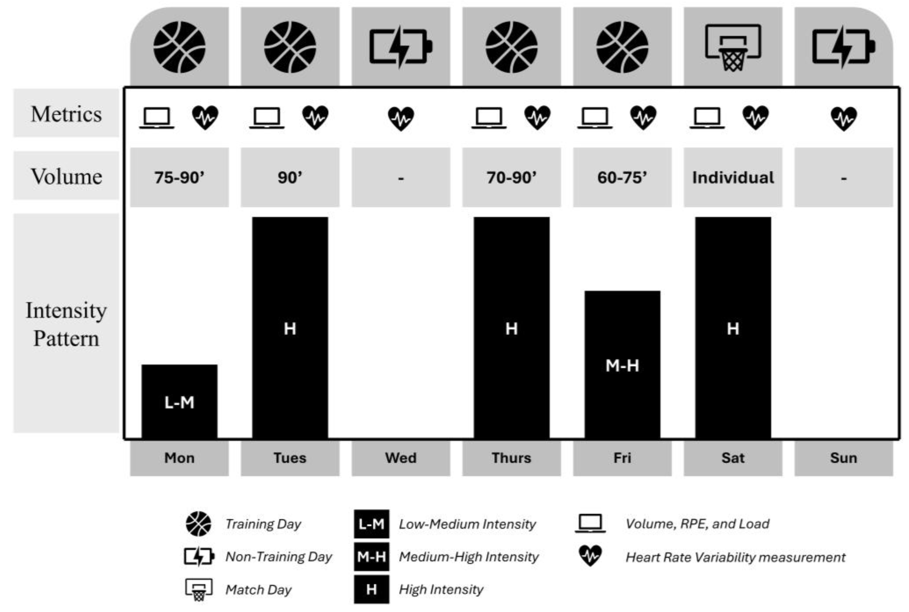
Figure 2.
Mean and standard error of natural logarithm of the root mean square of successive differences (LnRMSSD) as a function of the type of day: Match Day(MD), Training Day (TD) , or Non-Traininig Day (NTD). * Significant difference at p < 0.05.
Figure 2.
Mean and standard error of natural logarithm of the root mean square of successive differences (LnRMSSD) as a function of the type of day: Match Day(MD), Training Day (TD) , or Non-Traininig Day (NTD). * Significant difference at p < 0.05.
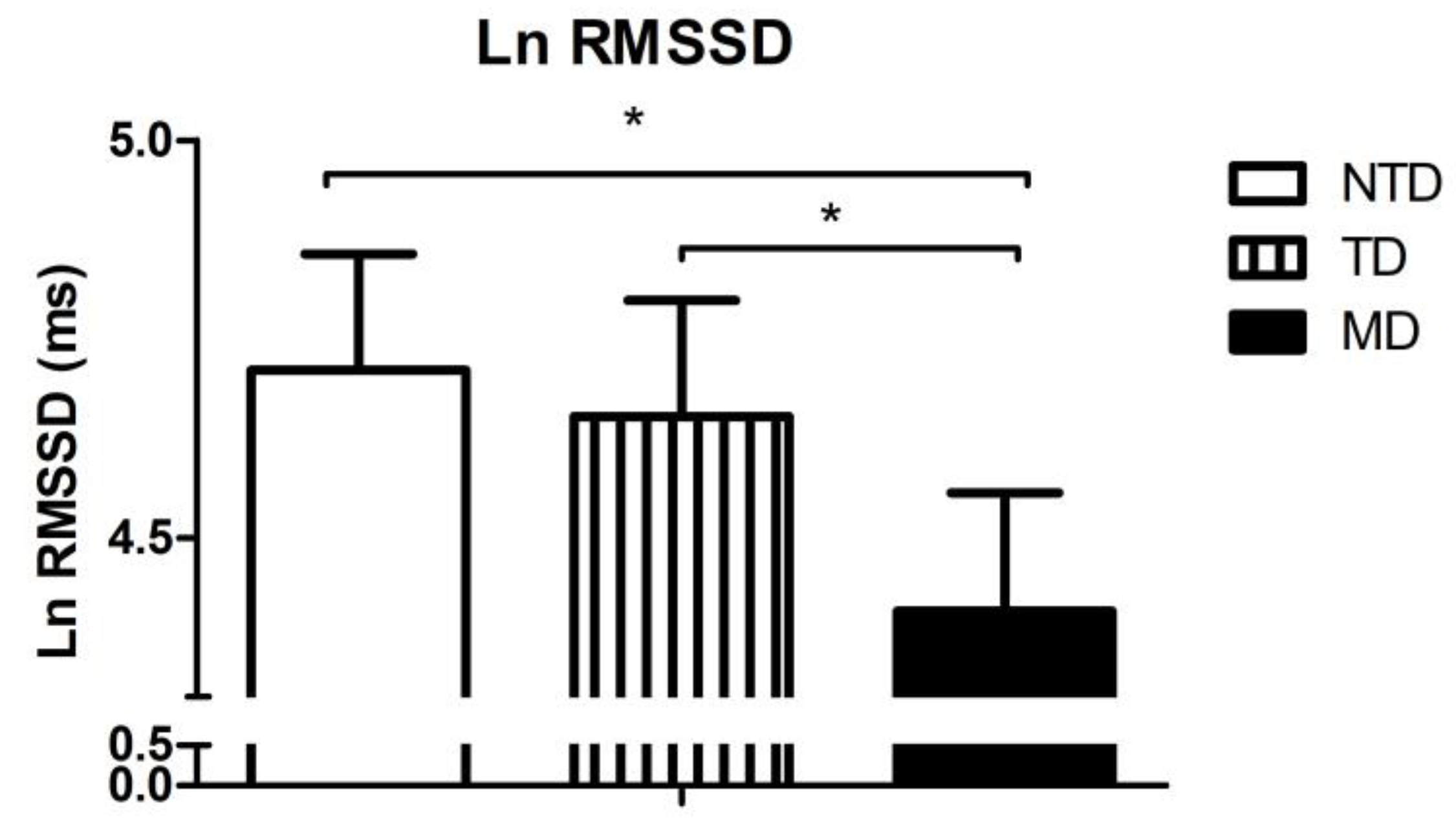
Figure 3.
Most relevant variables for characterizing LnRMSSD. The order indicates their importance in modifying LnRMSSD. Variables to the left of the Y-axis decrease LnRMSSD, while those to the right increase it. Red dots indicate high values of the variable, while blue dots indicate low values. The description of each abbreviation is provided in Table A1.
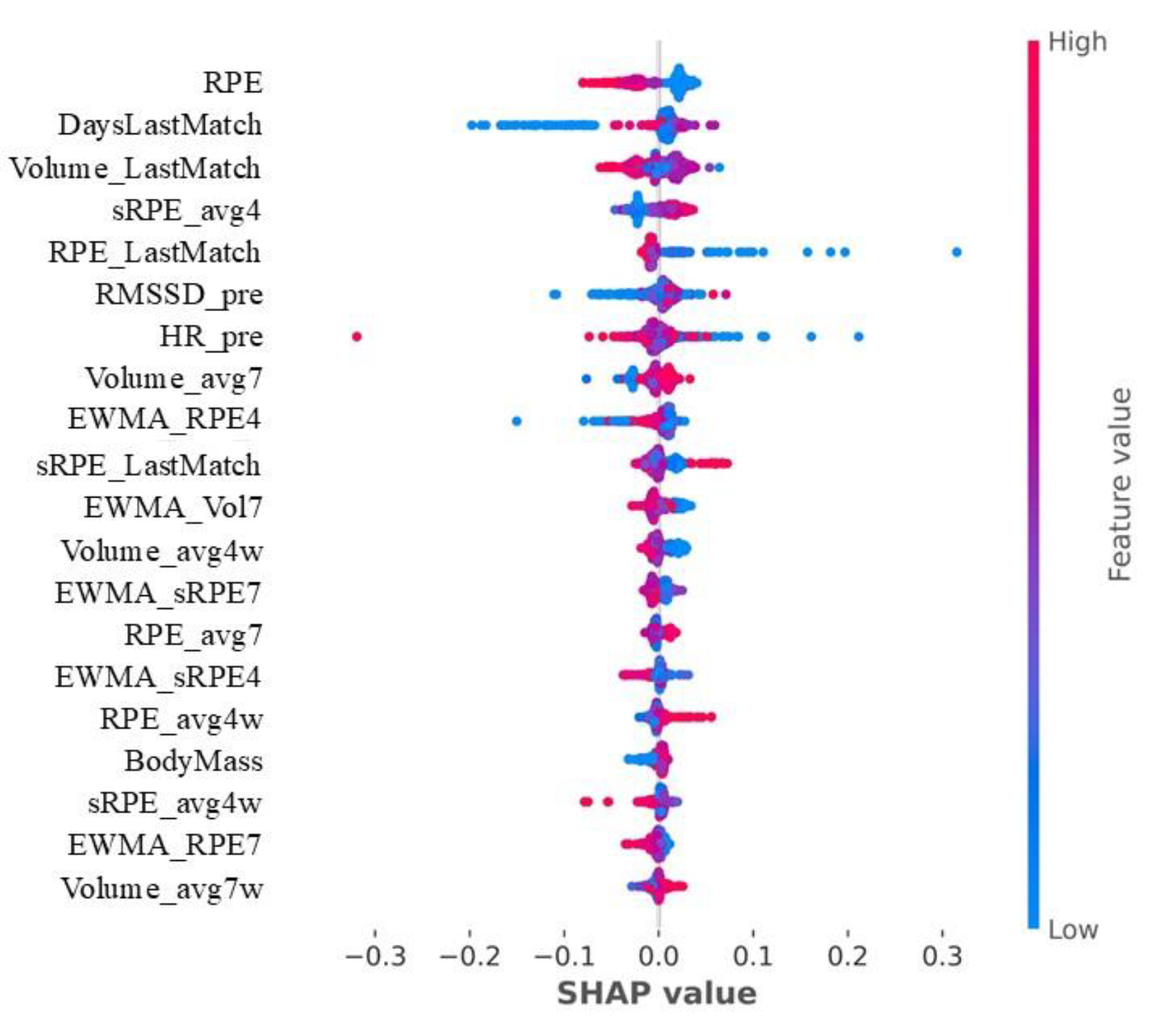
Figure 4.
Most relevant variables for characterizing LnRMSSD for each player. The description of each abbreviation is provided in Table A1.
Figure 4.
Most relevant variables for characterizing LnRMSSD for each player. The description of each abbreviation is provided in Table A1.
Disclaimer/Publisher’s Note: The statements, opinions and data contained in all publications are solely those of the individual author(s) and contributor(s) and not of MDPI and/or the editor(s). MDPI and/or the editor(s) disclaim responsibility for any injury to people or property resulting from any ideas, methods, instructions or products referred to in the content. |
© 2025 by the authors. Licensee MDPI, Basel, Switzerland. This article is an open access article distributed under the terms and conditions of the Creative Commons Attribution (CC BY) license (http://creativecommons.org/licenses/by/4.0/).
Copyright: This open access article is published under a Creative Commons CC BY 4.0 license, which permit the free download, distribution, and reuse, provided that the author and preprint are cited in any reuse.


