
Submitted:
12 August 2025
Posted:
13 August 2025
You are already at the latest version
Abstract
Accurate and scalable evaluation in team sports remains challenging, motivating the use of artificial‑intelligence models to support objective athlete assessment. This study develops and validates a predictive model capable of calibrated, operationally tested classification of team‑sport athletes as high‑ or low‑performance using a synthetic, literature‑informed dataset (n = 400). Labels were defined a priori by simulated group membership, while a composite score was retained for post‑hoc checks to avoid circularity. LightGBM served as the primary classifier and was contrasted with Logistic Regression (L2), Random Forest, and XGBoost. Performance was evaluated with stratified, nested 5×5 cross-validation. Calibrated, deployment-ready probabilities were obtained by selecting a monotonic mapping (Platt or isotonic) in the inner CV, with two pre-specified operating points: screening (recall-oriented; precision ≥0.70) and shortlisting (F1-optimized). Under this protocol, the model achieved 89.5% accuracy and ROC‑AUC 0.93. SHAP analyses indicated VO₂max, decision latency, maximal strength, and reaction time as leading contributors with domain‑consistent directions. These results represent a proof-of-concept and an upper bound on synthetic data and require external validation. Taken together, the pipeline offers a transparent, reproducible, and ethically neutral template for athlete selection and targeted training in team sports; calibration and pre‑specified thresholds align the approach with real‑world decision‑making.
Keywords:
artificial intelligence
; predictive modeling
; team sports
; LightGBM
; SHAP
; nested cross‑validation
; calibration
; talent identification
1. Introduction
In the modern landscape of team sports, accurately assessing and forecasting athletic performance has become both a practical challenge and a strategic priority. Coaches, analysts, and sport scientists continuously seek methods to identify performance potential early, personalize training interventions, and make informed decisions about athlete selection and development. Traditional methods such as field testing, observational assessment, and expert judgment, while valuable, often rely on limited, time-consuming, or subjective procedures. In contrast, data-driven techniques powered by artificial intelligence (AI) have emerged as promising tools to enhance performance evaluation by learning patterns across multiple athlete characteristics.
Recent advances in AI and machine learning allow predictive models to process complex relationships between physical, physiological, and cognitive factors and to infer performance outcomes with increasing accuracy. These approaches offer the advantage of speed, scalability, and objectivity - qualities that are particularly relevant in sports contexts where decisions must often be made under time constraints and with limited direct testing capacity. As such, predictive modeling is increasingly being recognized as a strategic asset in both elite and developmental sport environments.
This study presents a predictive modeling approach designed to estimate general athletic performance levels in team sport athletes using artificial intelligence. Rather than relying on real-world data collection, the study operates within a controlled simulation framework in which key performance-related variables are constructed and labeled to represent high- and low-performance profiles. By training and evaluating a supervised machine learning model on this dataset, the research aims to demonstrate that AI can meaningfully differentiate between performance levels, identify the most relevant predictors, and support practical use cases in athlete evaluation and early-stage decision-making.
The primary objective of this study is to construct and validate an AI-based predictive model capable of estimating athletic performance in a team sports context. The approach is proposed as a replicable and ethically neutral foundation for future research, tool development, and potential integration into sport selection and training systems.
To structure the evaluation of the modelling framework, a series of seven confirmatory hypotheses was prespecified, covering discrimination, comparative performance, calibration, operating thresholds, robustness, interpretability, and distributional validity. Each hypothesis is aligned with the simulation design and linked to specific performance targets, ensuring that the evaluation criteria remain transparent, reproducible, and relevant to practical decision-making. The hypotheses (H1–H7) are outlined below together with the quantitative or qualitative benchmarks used for their assessment:
- H1 – Discrimination. LightGBM attains ROC-AUC ≥ 0.90 with a lower 95% CI bound ≥ 0.85.
-
H2 – Comparative performance. LightGBM outperforms or matches:
- (a)
- L2-regularized Logistic Regression;
- (b)
- Random Forest;
- (c)
- XGBoost,
with ΔAUC ≥ 0.02 on average, or differences statistically indistinguishable (paired bootstrap one-sided p < 0.05), while retaining superior calibration (H3).
- 3.
-
H3 – Calibration. With monotone probability calibration (Platt or isotonic chosen in inner CV), the model achieves:
- (a)
- Brier ≤ 0.12;
- (b)
- calibration slope in [0.9, 1.1];
- (c)
- intercept in [−0.05, 0.05];
- (d)
- ECE ≤ 0.05
across outer folds (pass if ≥ 4/5 folds).
- 4.
-
H4 – Operational thresholds. Using calibrated probabilities, the two operating points meet:
- (a)
- Screening: Recall ≥ 0.90 with Precision ≥ 0.70;
- (b)
- Shortlisting: F1 ≥ 0.88.
- 5.
- H5 – Imbalance robustness. Under a 30/70 imbalance scenario, PR-AUC ≥ 0.85 and the top 5 SHAP features preserve rank order up to Kendall’s τ ≥ 0.70 vs. the balanced setting.
- 6.
- H6 – Stability of explanations. Global SHAP importance is stable across folds (median Spearman ρ ≥ 0.80 for the top 8 features), consistent with Permutation Importance (ρ ≥ 0.70). All ALE shows domain-consistent directionality for VO₂max ↑, Max Strength ↑, Decision Latency ↓, Reaction Time ↓.
- 7.
- H7 – Distributional validity. Kolmogorov–Smirnov tests against empirical references (variable-appropriate transforms; Holm correction) show no rejections at α = 0.05; otherwise, generation parameters are revised prior to training.
Exploratory analyses - decision curve analysis (net benefit), threshold sensitivity (±0.05 probability), and composite-score correlations (post hoc convergent check).
1.1. Literature Review
In recent decades, the integration of artificial intelligence (AI) into sports analytics has transformed athlete evaluation and performance prediction methodologies [1,2]. This shift from traditional assessment methods toward data-driven predictive modeling is motivated by the demand for objectivity, efficiency, and enhanced decision-making precision in athlete development and selection processes [3]. Numerous studies highlight the efficacy of AI algorithms, such as decision trees, random forests, neural networks, and gradient boosting machines, in accurately predicting athletic performance across diverse sports contexts [4,5].
AI-driven performance prediction primarily leverages large datasets comprising physiological, biomechanical, and cognitive variables to construct predictive models capable of differentiating athlete performance levels [6,7]. Physiological variables, particularly aerobic capacity (VO₂max), muscular strength, and heart rate recovery, have consistently emerged as robust predictors of athletic success, as evidenced by extensive empirical research. VO₂max, for example, has been widely validated as a critical determinant of aerobic endurance, directly correlating with sustained physical effort capabilities in endurance-based sports [8,9,10].
Biomechanical attributes, including acceleration, agility, and explosive power, also play critical roles in determining athletic performance, especially in dynamic team sports. Studies employing biomechanical metrics such as sprint acceleration times, countermovement jump heights, and agility performance indices have repeatedly confirmed their predictive validity and practical relevance [11,12]. The integration of biomechanical parameters within predictive models facilitates more nuanced and sport-specific athlete assessments, thus enhancing their predictive accuracy and applicability [13,14,15].
Recently, cognitive and psychological factors have gained recognition for their significant predictive value in athletic contexts. Decision-making latency, reaction time, and attentional control have been extensively studied and validated as critical performance determinants, particularly within fast-paced team sports requiring rapid cognitive processing and adaptive responses [16,17,18]. Empirical findings underscore that faster decision-making and quicker reaction times correlate strongly with superior performance outcomes, emphasizing the importance of incorporating cognitive parameters within predictive models. Integrating these cognitive metrics with established physiological and biomechanical predictors within AI-based frameworks has been shown to significantly improve classification accuracy and enhance the interpretability of athlete performance models in team sport contexts [19,20].
Machine learning techniques have been successfully applied to performance prediction across various team sports, demonstrating robust capabilities in athlete classification and selection processes. Among these techniques, Light Gradient Boosting Machines (LightGBM) and Extreme Gradient Boosting (XGBoost) algorithms have shown exceptional predictive accuracy and efficiency, often outperforming traditional statistical models. These methods handle large and complex datasets effectively, facilitating precise identification of key performance predictors and enhancing interpretability through feature importance analyses [21,22,23]. Compared to other popular machine learning methods, the Light Gradient Boosting Machine (LightGBM) offers clear advantages in predicting sports performance due to its high computational efficiency and excellent capability to handle large and complex structured datasets. The algorithm provides superior predictive accuracy and advanced interpretability through methods such as SHAP. Such gradient boosting approaches have already demonstrated strong performance in talent identification tasks, making them particularly well suited to the multidimensional predictor structure applied in the present study [24,25].
In team sports contexts specifically, studies utilizing AI-driven predictive models have demonstrated substantial improvements in athlete selection and performance optimization. For instance, predictive modeling has successfully classified professional football players based on their injury risk, performance trajectory, and training responsiveness, thus enabling targeted interventions [26,27,28]. Similarly, basketball and rugby research employing machine learning approaches report high classification accuracy and strong predictive performance, reinforcing the practical utility and effectiveness of AI in athletic evaluation [29,30].
Despite significant advancements, the predictive accuracy of AI models depends heavily on the quality and representativeness of the input data. Synthetic data generation, although methodologically sound and ethically advantageous, introduces limitations regarding generalizability and ecological validity. Nevertheless, synthetic datasets allow controlled experimental conditions, systematic variation of key parameters, and rigorous validation procedures, thereby offering substantial methodological advantages for predictive modeling research [31,32,33,34,35].
Interpretability of AI models remains a critical aspect influencing their practical adoption in sports contexts. Recent advances, particularly the development of SHAP (Shapley Additive Explanations) analysis, have significantly improved the transparency and interpretability of complex predictive models [36,37]. SHAP provides detailed insights into how specific variables influence individual and collective predictions, thus enhancing the practical utility, trustworthiness, and applicability of AI models in athletic performance analysis [38,39,40].
The application of AI-driven predictive models in talent identification processes has been particularly impactful, revolutionizing traditional selection paradigms. Research indicates that predictive models employing comprehensive physiological, biomechanical, and cognitive data outperform conventional selection methods based on subjective expert evaluations. This transition towards data-driven, objective evaluation frameworks holds substantial implications for athlete development programs, recruitment strategies, and long-term performance optimization [41,42,43]. In the specific context of talent identification in competitive team sports, prior research has applied machine learning to distinguish high- from lower-performing athletes based on multidimensional performance profiles. However, most of these studies have relied on relatively small real-world datasets, often lacking external validation and comprehensive interpretability analyses [44,45].
Cross-validation procedures are integral to validating AI model performance and ensuring generalizability. Methodological rigor involving repeated cross-validation (e.g., five-fold, ten-fold) significantly enhances confidence in model robustness, predictive stability, and reliability [46,47,48]. Studies employing rigorous cross-validation consistently report superior generalizability and applicability across different athlete populations, underscoring the critical importance of validation methods in predictive modeling research [49,50].
Effect size analysis and statistical validation methods (e.g., independent t-tests, Cohen’s d) further reinforce the scientific robustness of predictive modeling studies. The combination of AI-driven classification results with rigorous statistical validation ensures that observed differences between performance groups are both statistically significant and practically meaningful, thereby strengthening the overall methodological credibility and practical relevance of predictive models.
While AI-driven predictive modeling demonstrates substantial potential and effectiveness, future research must address current limitations and methodological challenges. The primary challenge involves empirical validation with real-world athlete data to enhance ecological validity and practical applicability. Additional research comparing diverse machine learning algorithms and employing longitudinal designs will further elucidate methodological robustness and optimize model performance.
In conclusion, the integration of artificial intelligence into talent identification and performance prediction in competitive team sports represents a significant advancement in sports analytics, offering the potential to transform athlete selection and development. Addressing critical gaps in dataset representativeness, ecological validity, interpretability, and robustness under class imbalance, the present study employs a controlled synthetic-data approach combined with an interpretable machine learning framework (LightGBM with SHAP and ALE). This design provides an objective, reproducible, and ethically neutral foundation for predictive modelling, enhancing methodological rigour, practical relevance, and applicability in real-world team sport contexts.
2. Materials and Methods
This study employed a controlled, simulation-based approach to assess the efficacy and feasibility of artificial intelligence (AI) techniques in predicting athletic performance in team sports contexts. To ensure replicability and ethical neutrality, real-world athlete data were not utilized. Instead, a detailed synthetic dataset was engineered, reflecting realistic physiological and cognitive athlete profiles relevant to competitive team sports.
Building on this design rationale, the methodological framework of this proof-of-concept study combines a simulation-based data design, a confirmatory hypothesis structure (H1–H7), and a sequential modeling pipeline for athlete classification in team sports. This pipeline operationalizes the framework through modular stages—from variable definition and synthetic data generation to model training, validation, calibration, and interpretability analyses. An overview of this workflow is presented in Figure 1, summarizing the key stages and logic of the simulation-based approach.
Figure 1 provides an overview of the sequential workflow applied in this proof-of-concept study, covering all stages from variable definition to model interpretation. The process began with the identification of key performance indicators across physiological, biomechanical, and cognitive-psychological domains, based on targeted literature review. A synthetic, literature-informed dataset (n = 400) was generated to emulate realistic athlete profiles, with distributional validity confirmed using Kolmogorov–Smirnov screening. Preprocessing steps included data quality checks, imputation where required, and correlation assessment. Model development employed a nested stratified 5×5 cross-validation design, with Light Gradient Boosting Machines (LightGBM) as the primary classifier benchmarked against Logistic Regression (L2), Random Forest, and XGBoost. Probability calibration was performed within the inner loop using Platt scaling or isotonic regression, and two operational decision modes were defined—screening and shortlisting—aligned with common talent-identification scenarios. Model interpretability was addressed through SHAP-based feature importance, agreement with permutation importance, fold-to-fold stability analysis, and ALE plots for domain-consistent effect directions. Robustness analyses included class-imbalance stress-testing, sensitivity to imputation strategies, and preservation of top-feature rankings under variable perturbations. The following subsections expand on each stage of this workflow in the order shown in the figure, ensuring clarity and methodological transparency.
2.1. Study Design, Rationale, and Variable Selection
The present study employs a computationally-driven, simulation-based approach utilizing artificial intelligence (AI) for predictive modeling of athletic performance in team sports. The deliberate choice of synthetic datasets instead of field-based athlete data is fundamentally justified by methodological and ethical considerations. Synthetic data generation ensures complete ethical neutrality by eliminating privacy concerns associated with personal athlete data, while simultaneously offering full experimental control and replicability - both crucial for high-quality scientific research. The controlled computational environment allows precise manipulation of performance-related variables, systematic replication of conditions, and rigorous evaluation of predictive accuracy without real-world confounding factors.
Variable selection was performed following a rigorous review of contemporary sports-science literature, emphasizing the complexity and multidimensional nature of performance in team sports. Selected variables encompass three major domains of performance determinants: physiological, biomechanical, and cognitive-psychological. Physiological variables focusing on aerobic capacity, muscular strength, and recovery capability were included due to their strong empirical associations with sustained athletic performance, endurance during competitive play, and injury risk mitigation. These physiological characteristics have been consistently highlighted in team sports research as pivotal to athlete performance outcomes, underpinning both physical resilience and competitive efficacy.
Biomechanical performance indicators, specifically those related to linear acceleration, explosive lower-body power, and agility, were integrated into the model due to their established predictive validity concerning rapid movements, dynamic transitions, and reactive capabilities - actions extensively occurring in team-sport competitive scenarios. The biomechanical dimension is critically linked to an athlete's ability to effectively execute sport-specific movements under high-intensity conditions, significantly influencing competitive success and overall athletic efficiency.
Cognitive and psychological variables were deliberately included to capture the increasingly acknowledged cognitive determinants of athletic success, namely rapid decision-making, sustained attention control, and psychological resilience under pressure. Empirical evidence from recent cognitive-sport research highlights these factors as critical predictors of successful athletic performances, particularly in environments characterized by rapid cognitive demands, frequent decision-making under uncertainty, and intense competitive pressure.
Collectively, these strategically selected performance dimensions create a comprehensive and scientifically justified framework for robust predictive modeling of athletic performance in team sports. For clarity and ease of replication, Table 1 presents the selected performance-related variables along with their measurement units, value ranges, and the group-specific distribution parameters (mean ± SD) used during synthetic data generation.
To reflect field realities, variables were generated under a multivariate structure with domain-plausible inter-variable correlations (e.g., VO₂max with heart-rate recovery and CMJ; sprint with change-of-direction), measurement error at instrument level, truncation to physiologically plausible intervals with domain-appropriate rounding, and 8% global missingness (mixed MAR/MNAR). Missing values were imputed within cross-validation folds using Iterative Imputer (sensitivity: KNN).
These rigorously established parameters lay the groundwork for robust and valid predictive modeling, bridging the gap between scientifically grounded theoretical concepts and their meticulous methodological implementation. This approach allows for controlled manipulation of key performance indicators while preserving sport-specific realism, ultimately enabling the development of replicable and ethically sound AI-based evaluation frameworks.
2.2. Synthetic Dataset Generation, Validation and Labeling
The synthetic dataset employed in this study was systematically generated to simulate realistic athlete populations, accurately reflecting the diverse physiological and cognitive characteristics found in competitive team sports. A total of 400 virtual athlete profiles were created, providing an adequately large and statistically robust sample for training and validating the predictive modeling approach. We targeted n = 400 based on precision for AUC and Brier score under the assumed separability. A parametric bootstrap (B = 2000) indicated approximate 95% CI widths of ~0.06 for AUC and ~0.014 for Brier at prevalence 0.50, which we considered adequate for a proof-of-concept study.
To ensure ecological validity, each variable was generated using controlled random sampling from normal distributions, parameterized based on established physiological and cognitive norms sourced from recent empirical sports-science literature. Specifically, the virtual athletes were categorized into two performance groups: "high-performance" and "low-performance," each group comprising precisely 200 profiles. This balanced structure was intentionally chosen to facilitate robust binary classification and minimize potential biases during model training.
Generation Procedure - each performance-related variable (detailed previously in Section 2.1 and summarized numerically in Table 1) was assigned distinct distribution parameters (mean ± SD), defined separately for high- and low-performance groups. For instance, maximal oxygen uptake (VO₂max) for high-performing athletes was sampled from a distribution with a mean of 60 mL/kg/min (±5), whereas low-performing athletes had a mean of 40 mL/kg/min (±5). To stress-test the end-to-end pipeline and to facilitate interpretation checks, we intentionally set between-group differences to be large across several predictors (e.g., VO₂max, reaction/decision times, strength). As a result, many variables exhibit |Cohen’s d| > 2.5 (see Table 4), which is expected to inflate discrimination under cross-validation. The estimates reported here should therefore be read as an upper bound under favorable signal-to-noise conditions rather than as field-realistic performance. Analogously, other variables, including reaction times, sprint times, muscular strength, and cognitive indices, were generated using group-specific parameters informed by recent empirical data from elite and sub-elite team sport athlete cohorts.
Validation Procedure - The realism and marginal validity of the synthetic dataset were assessed with univariate Kolmogorov–Smirnov (KS) tests after variable-specific transformations and Holm correction. Synthetic distributions were compared with pre-specified empirical targets from the sports-science literature to check alignment with physiologically and cognitively plausible ranges. KS screening indicated alignment for 5 of 6 variables (Holm-adjusted p > 0.05) and a deviation for Decision Time (KS D = 0.437; Holm-adjusted p < 0.001). Because KS is a univariate test, non-rejection does not establish distributional equivalence nor multivariate alignment. Targets (distribution families and parameters) were pre-specified from the literature, and the generator was frozen prior to model training. Full statistics are reported in Table S1 (KS D, raw p, Holm-adjusted p), and representative Q–Q plots are shown in Figure S1 (in Supplementary Materials).
Multivariate dependence and copula-based generation - beyond matching marginal targets, we imposed a realistic cross-variable dependence structure using a Gaussian copula. A target rank-correlation (Spearman) matrix Rs was pre-specified from the literature and domain constraints. We then mapped Rs to the Gaussian copula correlation Rg via the standard relation Rg = 2 sin (πRs /6) and computed its nearest positive-definite approximation. Synthetic samples were drawn as z∼N(0,Rg) converted to uniform scores u=Φ(z) and finally transformed to the required marginals by inverse CDFs xj = Fj-1(uj) (with truncation where applicable). To avoid label leakage, class separation was induced only through location/scale shifts of the marginals while keeping the copula shared across classes.
Labeling - binary labels were defined a priori by simulated group membership (High-Performance vs. Low-Performance), using the group-specific parameters in Table 1 (n = 200 per group). The weighted composite score was retained only for post hoc convergent checks (distributional separation and threshold sensitivity) and did not influence labeling or model training. This design prevents circularity between features and labels and aligns with the two-group simulation.
Bias Considerations in Synthetic Data Generation - although KS screening aligned with targets for 5/6 variables and flagged a deviation for Decision Time (D = 0.437; Holm-adjusted p < 0.001), this should not be interpreted as distributional equivalence, particularly with respect to joint (multivariate) structure. The reliance on parametric normal generators and predetermined ranges—chosen for experimental control—may limit real-world heterogeneity and nonlinear effects, which can inflate between-group separations and suppress within-group variability. These modeling choices were intentional to stress-test the pipeline and ensure replicability in a proof-of-concept setting. As a result, the high signal-to-noise ratio and balanced classes (n = 200 per group) likely favor optimistic estimates of both discrimination and calibration (AUC/accuracy, Brier score, ECE). We therefore interpret all performance metrics as an upper bound and refrain from claiming external validity; prospective validation on empirical athlete cohorts is required prior to practical use.
2.3. Predictive Modeling, Optimization, and Evaluation
Objective and outcome - the predictive task was a binary classification of athlete profiles into High-Performance (HP) vs. Low-Performance (LP) groups. Labels were defined a priori by simulated group membership (HP = 1, LP = 0), consistent with the two-group design; the composite score was retained only for post hoc convergent checks and did not influence labeling or training. This design avoids circularity and preserves interpretability of evaluation metrics.
Leakage control and preprocessing - all preprocessing steps were executed strictly within cross-validation folds to prevent information leakage. Missing values (introduced by design) were imputed inside each training split using an iterative multivariate imputer (Bayesian ridge regression) applied column-wise, with numeric features standardised prior to imputation. Overall missingness ranged from 1% to 15% across variables. The fitted imputer was then applied to the corresponding validation/test split within the same fold. Where applicable, scaling/transformations were likewise fitted on training partitions only. Sensitivity to imputation method and to perturbations of the simulated correlation structure (Rs) was evaluated as described in sub-section 2.5, with results summarised in Supplementary Figure S4. Categorical encodings were not required; all predictors were continuous or ordinal.
Models compared - the primary classifier was Light Gradient Boosting Machine (LightGBM), selected for efficiency on tabular, potentially non-linear data with mixed feature effects. To contextualize performance, we evaluated three baselines under identical pipelines:
- 1)
- Logistic Regression (L2) with class-balanced weighting;
- 2)
- Random Forest;
- 3)
- XGBoost.
Hyperparameters for all models were tuned in the inner cross-validation (below), using comparable search budgets and early-stopping where applicable.
Nested cross-validation design - to obtain approximately unbiased generalization estimates, we employed a 5×5 nested cross-validation protocol: 5 outer folds for performance estimation and 5 inner folds for hyperparameter optimization via randomized search.
- Primary selection metric: Brier score (proper scoring rule for probabilistic predictions); ROC-AUC reported for discrimination; F1 used only as a tie-breaker for threshold metrics.
- Search budget: 100 sampled configurations per model (inner CV), with stratified folds.
- Early stopping: enabled for gradient-boosted models using inner-fold validation splits.
- Class balance: folds were stratified by HP/LP to preserve prevalence.
- Leakage control: all preprocessing (imputation, scaling/class-weights, and calibration selection: Platt vs. isotonic by Brier) was performed inside the training portion of each inner/outer fold; the test fold remained untouched.
The entire pipeline (imputation → model fit → probability calibration) was refit within each outer-fold training set, and predictions were produced on the corresponding held-out outer-fold test set.
Hyperparameter spaces (inner CV) - for each model we searched the following ranges (log-uniform where noted):
- Logistic Regression (LBFGS, L2). C ∈ [1e−4, 1e+3] (log-uniform); max_iter = 2000.
- Random Forest. n_estimators ∈ [200, 800]; max_depth ∈ {None, 3–20}; min_samples_leaf ∈ [1, 10];
- max_features ∈ {‘sqrt’, ‘log2’, 0.3–1.0}; bootstrap = True.
- XGBoost. n_estimators ∈ [200, 800]; learning_rate ∈ [1e-3, 0.1] (log-uniform); max_depth ∈ [2, 8];
- subsample ∈ [0.6, 1.0]; colsample_bytree ∈ [0.6, 1.0]; min_child_weight ∈ [1, 10]; gamma ∈ [0, 5];
- reg_alpha ∈ [0, 5]; reg_lambda ∈ [0, 5].
- LightGBM. num_leaves ∈ [15, 255]; learning_rate ∈ [1e-3, 0.1] (log-uniform); feature_fraction ∈ [0.6, 1.0]; bagging_fraction ∈ [0.6, 1.0]; bagging_freq ∈ [0, 10]; min_child_samples ∈ [10, 100]; lambda_l1 ∈ [0, 5]; lambda_l2 ∈ [0, 5].
Best models were selected by inner-CV Brier score (after post-hoc probability calibration), then refit on the outer-training fold.
Probability calibration and reporting metrics - because deployment decisions rely on well-calibrated probabilities, the inner CV selected between Platt scaling and isotonic regression based on Brier score on the inner validation data for the tuned model. The selection between Platt scaling and isotonic regression was made independently for each outer fold by choosing the mapping that achieved the lowest Brier score on the inner validation data. The chosen mapping was then refit on the full outer-fold training set and applied to the held-out test fold before evaluation. The chosen calibration mapping was then fit on the outer-fold training data and applied to the outer-fold test predictions. We reported, for each model:
- Discrimination: ROC-AUC (primary), PR-AUC;
- Calibration: Brier score, Expected Calibration Error (ECE), calibration slope and intercept;
- Classification metrics: accuracy, precision, recall, F1 (at selected thresholds; see below).
Calibration evaluation (outer folds) - for each outer fold and each model, we computed the (i) Brier score (mean squared error of probabilistic predictions), (ii) Expected Calibration Error (ECE) using K = 10 equal-frequency bins with a debiased estimator, and (iii) calibration-in-the-large (intercept) and calibration slope obtained from logistic recalibration of the outcome on the logit of predicted probabilities, i.e., logit(P(Y=1)) = β₀ + β₁ · logit( p̂ ), p̂ ∈ [10⁻⁶, 1−10⁻⁶]. Lower Brier/ECE indicate better calibration; ideal values are slope ≈ 1 and intercept ≈ 0. Post-hoc calibration (Platt or isotonic) was selected in the inner CV for the tuned model and then refit within the outer-fold training set before scoring on the held-out outer test set. We report fold-wise metrics and mean±SD across outer folds (Tabless 3a–3c).
Performance was summarized as the mean across outer folds with 95% bootstrap confidence intervals (B = 2000) and the fold-to-fold standard deviation. Confidence intervals were computed using the bias-corrected and accelerated (BCa) bootstrap method. Expected Calibration Error (ECE) was estimated using 10 equal-width probability bins, with a debiased estimator applied to aggregated predictions across outer folds.
Operating thresholds and decision analysis - for practical use, we defined two pre-specified operating points on calibrated probabilities:
- Screening — prioritize recall, constraining precision ≥ 0.70 to minimize missed HP athletes;
- Shortlisting — maximize F1 to balance precision and recall for final selections.
For both thresholds we report confusion matrices and derived metrics aggregated across outer folds, and we generate Decision Curve Analysis to quantify net benefit across a clinically plausible threshold range.
Robustness to class imbalance - to assess stability under realistic prevalence shifts, we replicated the entire nested-CV protocol on a 30/70 (HP/LP) imbalanced variant of the dataset (labels unchanged; sampling weights applied where appropriate). We report paired differences in PR-AUC, threshold-specific metrics, and agreement in feature influence, with emphasis on maintaining ranking stability among the top predictors. For each operating point, we report PRAUC, precision, recall, and F1 under a 30/70 prevalence scenario, using the same probability thresholds as in the balanced setting. We also computed Kendall’s τ correlation and its 95% confidence interval for the top-8 feature rankings between the 30/70 and balanced settings to assess stability in variable importance.
Statistical inference and uncertainty quantification - between-model comparisons used paired bootstrap on outer-fold predictions to estimate ΔAUC and obtain one-sided p-values where appropriate. All endpoints are provided with point estimates and 95% CIs; inference emphasizes interval estimates over dichotomous significance decisions. Additional group-comparison statistics (independent samples t-tests, Cohen’s d) are reported separately for descriptive context, independent of model training.
Implementation note - the pipeline was implemented in Python 3.10 using NumPy/Pandas for data handling, scikit-learn for CV, imputation, calibration and metrics, LightGBM/XGBoost for gradient boosting, and SHAP for interpretability. All transformations, tuning and calibration were fold-contained; random seeds were set for reproducibility.
2.4. Feature Importance, Interpretability, and Technical Implementation
Understanding and interpreting the contributions of individual variables to predictive performance outcomes is essential for translating machine learning models from theoretical exercises into practical tools applicable in sports contexts. To achieve comprehensive interpretability, the current study incorporated feature importance analysis and Shapley Additive Explanations (SHAP), two complementary approaches renowned for providing robust insights into the decision-making logic of complex predictive models such as LightGBM.
Feature importance analysis within the LightGBM framework was initially conducted based on gain values, quantifying each variable’s contribution to overall predictive model accuracy. Variables exhibiting higher gain values are identified as more influential predictors of athletic performance. However, recognizing that feature importance alone provides limited context regarding the directionality or nuanced contributions of individual variables, additional interpretative analyses were conducted using SHAP methodology.
SHAP is a game-theoretic interpretability framework, widely recognized for its efficacy in quantifying variable contributions to individual predictions as well as global model behaviors. SHAP values provide precise, interpretable metrics reflecting how and why specific variables influence predictive outcomes, offering insights into both the magnitude and direction (positive or negative) of effects. This approach allowed detailed exploration and clear visualization of the predictive relationships identified by the model, revealing the relative impact of physiological, biomechanical, and cognitive-psychological variables on performance classifications. Consequently, the SHAP analysis not only strengthened the interpretability and credibility of the predictive findings but also enhanced the practical applicability of the model, enabling coaches, practitioners, and researchers to better understand the underlying determinants of athletic success and target interventions more effectively.
To evaluate the stability of global explanations, we computed Spearman’s rank correlation coefficient (ρ) between the mean absolute SHAP values of all features across each pair of outer folds, generating a 10×10 correlation matrix. The stability score was defined as the mean off-diagonal ρ, representing the average agreement in feature importance rankings between folds. Agreement between SHAP-based and permutation-based importance rankings was quantified using Kendall’s τ, tested for significance via a permutation test (B = 2000). Sign consistency was calculated as the proportion of folds in which each feature’s mean SHAP value retained the same sign (positive or negative) as in the majority of folds. All stability computations were based on SHAP values aggregated from the outer-fold test predictions.
Because interpretability workflows may involve multiple simultaneous hypotheses (e.g., correlations between raw features and SHAP values across outer folds, directional tests on ALE/PDP curves, or comparisons of SHAP distributions between groups), we controlled the family-wise error rate using the Holm (step-down) procedure. Unless specified otherwise, p-values reported for interpretability-related tests are Holm-adjusted within each family of features analyzed for a given endpoint, ensuring robust inference without unduly inflating Type I error.
From a technical implementation perspective, the entire predictive modeling pipeline - including synthetic dataset generation, data preprocessing, model training, validation, hyperparameter optimization, and interpretability analyses - was executed using Python 3.10, a widely accessible and open-source programming environment. Core scientific libraries employed included NumPy and Pandas for efficient data handling and preprocessing, Scikit-learn for dataset partitioning and cross-validation procedures, LightGBM for predictive modeling, and the official SHAP library for interpretability analyses.
All computational procedures were conducted on a standard desktop workstation featuring an Intel Core i7 processor and 32 GB of RAM, intentionally excluding GPU acceleration to demonstrate methodological accessibility, scalability, and reproducibility in typical academic or applied settings. To further ensure complete methodological transparency and reproducibility of findings, all random sampling processes utilized a fixed random seed (42), and comprehensive Python scripts documenting every analytical step (from dataset creation to model evaluation and interpretability) are available upon reasonable request, enabling precise replication, validation, and extension of this research by the broader scientific community.
2.5. Statistical Analyses (Group Comparisons)
Group-level comparisons between High-Performance (HP) and Low-Performance (LP) profiles were conducted for descriptive context and construct validity only, independently of model training. For each primary variable, we report independent-samples t-tests (Welch’s correction if Levene’s test indicated unequal variances), Cohen’s d with 95% CIs, and two-sided p-values. Normality was inspected via Q–Q plots; where deviations were material, results were confirmed with Mann–Whitney U tests (conclusions unchanged). These analyses support the interpretation of model-identified predictors and do not affect labeling or cross-validation procedures.
To account for multiple comparisons across the eight primary variables, Holm correction was applied within each family of tests; we report both unadjusted and Holm-adjusted p-values where relevant. These descriptive comparisons further contextualize the predictive findings, reinforcing the practical relevance of the key performance indicators highlighted in this study. Applying this level of statistical control strengthens the reliability of the reported effects and ensures that the observed differences are both statistically sound and practically meaningful.
3. Results
The predictive model exhibited exceptional accuracy and robustness in classifying athletes into high- and low-performance groups, demonstrating its practical applicability and effectiveness. Comprehensive performance metrics and insightful feature analyses validate the model's predictive strength, offering valuable implications for athlete evaluation and talent identification processes.
3.1. Predictive Model Performance
The performance of the Light Gradient Boosting Machine (LightGBM) predictive model was comprehensively evaluated using multiple standard classification metrics, ensuring rigorous assessment of its capability to distinguish effectively between high- and low-performance athlete profiles.
To ensure a robust and interpretable evaluation of the model’s predictive capacity, a comprehensive set of performance indicators was analyzed-capturing not only classification outcomes but also measures of consistency and generalizability. Table 2 presents these metrics in an extended and structured format, highlighting their statistical quality, operational relevance, contribution to error mitigation, and acceptable performance thresholds within the context of athlete selection.
These tabular insights are further reinforced by validation results and visualized model performance, which confirm the high classification quality and discriminative strength of the predictive framework.
The classification results, derived under stratified validation, demonstrated strong predictive accuracy and reliability, further confirming the robustness and practical utility of the developed model.
The model achieved an overall classification accuracy of 89.5%, indicating a high proportion of correct athlete classifications. In addition, it exhibited excellent discriminative capability, as evidenced by an AUC-ROC score of 0.93 - highlighting its effectiveness in reliably distinguishing between high- and low-performance athletes across a range of classification thresholds.
Additionally, the predictive model demonstrated high levels of both specificity and sensitivity. The precision reached 90.2%, indicating that the majority of athletes identified as high-performance were correctly classified. The model’s recall (sensitivity) was similarly robust at 88.7%, showing that it successfully captured a substantial proportion of truly high-performing athletes. The balanced performance of the model, as reflected by an F1-score of 89.4%, further emphasized the strong alignment between precision and recall—reinforcing the model’s efficacy and practical reliability in real-world classification scenarios.
Because real decisions hinge on explicit error trade-offs, two probability thresholds were prespecified on the calibrated outputs to reflect common use cases. A recall-oriented screening setting minimizes missed high performers and yields 92.0% recall with 81.1% precision (F1 = 86.2%), appropriate for early triage when sensitivity is prioritized. A shortlisting setting balances retrieval and over-selection at the final decision stage and corresponds to 90.2% precision, 88.7% recall, and F1 = 89.4%, aligning with the headline performance profile, with the corresponding counts and derived metrics.
Calibration diagnostics of the calibrated LightGBM showed close agreement between predicted and observed probabilities across outer folds. Reliability diagrams indicated only minor deviations from identity, and fold-wise calibration slope and intercept fell within the prespecified bounds (|intercept| ≤ 0.05; slope ≈ 1), with ECE remaining small. These results support the use of the two prespecified operating points on calibrated probabilities for decision-making.
To make the error trade-offs concrete, calibrated predictions were evaluated at the two operating points introduced above. Table 2b reports the confusion matrices for a recall-oriented screening setting—where sensitivity is kept high while respecting a minimum precision constraint—and for a shortlisting setting, where the F1-optimised cut-off balances retrieval and overselection.
The confusion matrices in Table 2b illustrate the trade-offs between recall and precision for the two prespecified decision settings. In the screening configuration, more candidates are flagged to minimize missed high performers, while the shortlisting configuration balances retrieval and overselection for final decisions. To complement these operational results, Table 2c presents the calibration performance of baseline models under the same outer-fold protocol, providing a comparative context for interpreting LightGBM’s outputs.
Values are reported as mean ± SD across the five outer folds in the nested 5×5 cross-validation. All baseline models were trained, tuned, and post-hoc calibrated under the same pipeline as LightGBM, ensuring a coherent comparison. Metrics include the Brier score and Expected Calibration Error (ECE, K = 10 equal-frequency bins, debiased), along with calibration slope and intercept (ideal slope ≈ 1, intercept ≈ 0). “Selected calibration” indicates whether Platt scaling or isotonic regression was chosen in the inner CV. This summary provides the calibration context for interpreting LightGBM’s operational results in Table 2 and Table 2b.
To complement the calibration summaries reported in Table 2c, Table 2d presents the direct comparative performance between LightGBM and each baseline model in terms of discrimination (ROC-AUC) and calibration (Brier score), including paired differences, confidence intervals, and statistical significance from outer-fold predictions.
The comparative analysis in Table 2d shows that LightGBM consistently outperformed all baseline models in both discrimination and calibration metrics, with all ΔAUC values positive and all ΔBrier values negative. These findings meet the pre-specified H2 criterion of achieving at least a 0.02 improvement in ROC-AUC or a statistically indistinguishable difference while maintaining superior calibration performance.
A comprehensive visual representation of these results is presented in Figure 2, combining a detailed Receiver Operating Characteristic (ROC) curve and an illustrative bar chart highlighting the specific performance metrics. The ROC curve visually demonstrates the exceptional discriminative capability of the model, while the adjacent bar chart succinctly conveys the quantitative values of each performance metric, enhancing both clarity and interpretability of the findings.
These findings collectively validate the predictive modeling approach as robust, precise, and applicable for practical utilization in athletic performance evaluation and selection contexts. Panel (A) presents all critical predictive metrics explicitly, while Panel (B) visually illustrates only the ROC curve, as this metric uniquely allows a graphical representation of the model's discriminative capability across various classification thresholds.
3.2. Feature Importance and SHAP Analysis
To gain deeper insights into the predictive mechanisms of the LightGBM model, an extensive feature importance analysis was conducted using both the traditional gain-based ranking method and Shapley Additive Explanations (SHAP). While gain values indicate each variable’s overall contribution to the predictive accuracy of the model, SHAP values provide detailed interpretative insights into how individual variables influence classification decisions globally and at the level of specific predictions. Analyses are aggregated across outer folds, with global rankings computed on mean absolute SHAP values.
Table 3 presents the top eight predictors ranked according to SHAP importance, alongside the mean differences observed between high-performance and low-performance athlete groups, the absolute differences (Δ), and the statistical effect sizes quantified by Cohen’s d, calculated based on simulated distributions. These data offer empirical evidence illustrating how SHAP-derived importance aligns closely with the actual differences identified between the two performance groups.
Consequently, the variables with the highest SHAP values - VO₂max, decision latency, maximal strength, and reaction time - also demonstrated the most pronounced absolute differences and clear statistical effects between groups (Cohen’s d > 3.5). The convergence between model-derived importance and statistical separation supports the robustness and validity of the predictive approach. The remaining analyzed variables, including countermovement jump height, sprint time, stress tolerance, and attention control, significantly contributed to the predictive performance of the model, underscoring the complex and multidimensional nature of athletic performance.
Therefore, SHAP analysis not only confirms the relative importance of individual variables in predicting performance but also provides explicit details regarding the directionality of each variable’s influence on athlete classification into high- or low-performance categories. Detailed results of this analysis are systematically presented in Table 3.
The results of the global feature importance analysis based on gain values computed by LightGBM highlighted several key predictors of athletic performance. Aerobic capacity (VO₂max), decision latency, maximal strength, reaction time, and countermovement jump height (CMJ) emerged as particularly influential variables, confirming their well-documented predictive relevance in team sports performance research.
Complementing traditional feature importance analysis, SHAP provided additional insights into both the magnitude and directionality of each variable’s impact on predictive outcomes. For instance, higher values of VO₂max and maximal muscular strength positively influenced athlete classification into the high-performance category, whereas increased decision latency and prolonged reaction time negatively affected performance classification.
These predictive relationships are clearly illustrated in Figure 3, which visually presents the relative importance of variables in athlete performance classification and explicitly demonstrates how variations in each variable influence model predictions.
These findings confirm the significance of a multidimensional predictive approach and emphasize the importance of integrating physiological, biomechanical, and cognitive variables into comprehensive athletic performance evaluation. The observed correlations in panel (B) further support the validity and relevance of the variables highlighted by the SHAP analysis, clearly indicating pathways for optimizing athlete selection and targeted development strategies. Where inferential checks were applied to interpretability outputs, p-values were Holm-adjusted within the corresponding feature family to control family-wise error without overstating significance.
3.3. Comparative Analysis of High- and Low-Performance Groups
To provide further insights into the discriminative capability of the predictive model and validate its practical utility, a detailed statistical comparison was conducted between high-performance (n = 200) and low-performance (n = 200) athlete profiles. This analysis focused specifically on the eight most influential variables identified through the SHAP analysis. Independent samples t-tests were used to evaluate between-group differences, with statistical significance set at p < 0.05. Additionally, Cohen’s d effect sizes were calculated to quantify the magnitude and practical relevance of the observed differences.
The results revealed statistically significant and practically meaningful differences across all eight analyzed performance variables. Notably, aerobic capacity (VO₂max) showed substantial between-group differences (high-performance: M = 58.5 ± 4.3 mL/kg/min; low-performance: M = 41.3 ± 5.1 mL/kg/min; p < 0.001, d = 3.65), highlighting its critical role in differentiating athletic potential. Similarly, decision latency (d = –4.20), reaction time (d = –4.21), and maximal strength (d = 3.49) exhibited large effects closely aligned with the model’s predictions. Other analyzed variables—countermovement jump height (d = 3.00), sprint time (d = –2.55), stress tolerance (d = 3.38), and attention control (d = 3.11)—also demonstrated robust differences, confirming their relevance within the athlete performance profile.
Negative Cohen’s d values (e.g., decision latency, reaction time, sprint time) indicate higher scores for the low-performance group, reflecting an inverse relationship with athletic performance. Complete statistical details are summarized comprehensively in Table 4.
Further reinforcing these statistical findings, the five-fold cross-validation procedure indicated consistent robustness and stability of the predictive model. The mean accuracy across folds was 89.2%, with a narrow 95% confidence interval (88.1% to 90.3%) and low standard deviation (0.9%), demonstrating the reliability and generalizability of the model across diverse subsets of data.
To enhance visual clarity and facilitate a comprehensive interpretation of these results, Figure 4 systematically illustrates the comparative analysis of all eight variables identified through SHAP analysis and statistical validation. The clear visual separation between high-performance and low-performance athlete groups across each variable emphasizes their strong discriminative ability, underscores their relevance within the predictive model, and highlights their practical importance for talent identification and targeted athletic training.
These visualizations underscore the pronounced differences between high-performance and low-performance athlete profiles across all key variables analyzed, reinforcing the robustness and practical efficacy of the predictive model developed and validated in this study. The results emphasize the importance of a multidimensional approach and the relevance of applying artificial intelligence to athletic performance evaluation and talent identification.
Collectively, these statistical analyses and visualizations validate the practical significance of the predictive modeling approach, clearly demonstrating its efficacy in distinguishing athlete performance levels and underscoring its applicability in athlete evaluation, selection, and targeted training interventions.
3.4. Hypotheses—Linkage to Results (H1–H7)
The results converge toward a clear conclusion: the model consistently distinguishes between high and low performance, calibrated probabilities support operational decisions in two distinct stages, and the key identified factors align with established benchmarks in sports science. The coherence between predictive performance, variable relevance, and effect direction provides the analysis with interpretive strength that reinforces the validity of the entire framework. On this basis, the hypotheses are examined individually in relation to the presented evidence:
H1 — Discrimination (primary endpoint): under stratified fivefold validation, LightGBM achieved an ROC-AUC of 0.93, indicating strong threshold-independent separation between high- and low-performance profiles. Accuracy of 89.5% further confirms consistent correct classification across folds. Model selection and post-hoc calibration followed the prespecified nested 5×5 cross-validation workflow, ensuring that these headline results are supported by a rigorous, leakage-controlled evaluation process. These findings exceed the AUC ≥ 0.90 target and confirm that H1 is fully satisfied.
H2 — Comparative performance (LGBM vs. LR/RF/XGB): all baseline models were processed under the same nested 5×5 pipeline, with post-hoc monotonic calibration selected in the inner CV. Their outer-fold calibration summaries are shown in Table 2c, while Table 2d reports discrimination and calibration metrics relative to LightGBM. Paired bootstrap analysis (B = 2000) yielded consistent positive ΔAUC values: vs LR, ΔAUC = 0.046 [95% CI: 0.024–0.068], p = 0.001; vs RF, ΔAUC = 0.032 [95% CI: 0.014–0.050], p = 0.004; vs XGB, ΔAUC = 0.019 [95% CI: 0.003–0.035], p = 0.038. Corresponding ΔBrier values were all negative, indicating lower calibration error for LightGBM: vs LR, ΔBrier = –0.009 [95% CI: –0.014 to –0.004], p = 0.002; vs RF, ΔBrier = –0.006 [95% CI: –0.010 to –0.002], p = 0.006; vs XGB, ΔBrier = –0.004 [95% CI: –0.008 to –0.001], p = 0.041. These results confirm that LightGBM meets or exceeds the comparative performance thresholds specified in the analysis plan, satisfying H2.
H3 — Calibration: Table S3d (Supplementary Materials) reports fold-wise Brier scores, ECE, calibration slope, and intercept for LightGBM, along with the calibration mapping selected in each fold. All mean values met the pre-specified targets (Brier ≤ 0.12, slope in [0.9, 1.1], intercept in [–0.05, 0.05], ECE ≤ 0.05), with low variability across folds. The reliability diagram in Figure X shows close agreement between predicted and observed probabilities, confirming that the calibrated outputs are well-suited for operational decision-making. These results satisfy H3.
H4 — Operational thresholds (screening and shortlisting): both pre-specified operating points achieved their target performance levels (Table 2b). The mean probability threshold for screening was 0.431 ± 0.015, while for shortlisting it was 0.587 ± 0.018 across outer folds (Supplementary Table S4). The associated Precision–Recall curves, F1–threshold profiles, and Decision Curve Analysis are presented in Supplementary Figure S2, illustrating the trade-offs and net benefit of each decision strategy.
H5– Robustness to class imbalance (30/70): the modelling framework was designed to maintain decision quality under changes in prevalence, and the 30/70 scenario confirmed that key predictive signals remained stable. Supplementary Table S5 shows that, under the 30/70 prevalence scenario, the model maintained high PRAUC values (screening: 0.881; shortlisting: 0.872), with precision, recall, and F1 closely matching those from the balanced setting. The Kendall’s τ between the top-8 feature rankings in the two scenarios was 0.88 [95% CI: 0.83–0.93], indicating strong stability in variable importance ordering. These results confirm that the approach preserves its practical utility even when the high-performance class is substantially under-represented, satisfying the robustness objective for H5. See also Supplementary Figure S3 for a visual comparison between the balanced and 30/70 settings.
Sensitivity analyses indicated minimal variation in performance across imputation strategies, with PRAUC differences below 1% between methods. Perturbations of Rs up to ±20% induced only small changes in PRAUC (≤0.7%). A priori power analysis confirmed that n = 400 provides >80% power to detect correlations as low as ρ = 0.15 at α = 0.05 (two-sided). These results are summarised in Supplementary Figure S4.
H6 — Stability and consistency of explanations: across outer folds, the most influential features—VO₂max, decision latency, maximal strength, and reaction time—consistently appeared at the top of the rankings, with directions of effect aligned to domain expectations. Stability analysis yielded a mean Spearman’s ρ of 0.91 ± 0.04, indicating high consistency in SHAP-based feature rankings between folds. Agreement with permutation importance rankings was also high (Kendall’s τ = 0.78, p < 0.001). Sign consistency exceeded 90% for all top-10 features and was above 95% for the top six. These findings are summarised in Figure 5, which illustrates the most important features by SHAP values, their stability across folds, the agreement between SHAP and permutation importance rankings, and the consistency of effect signs. The high stability metrics and strong agreement confirm H6, indicating that the explanation stability and consistency criteria were met.
H7 — Distributional validity (KS screening): Kolmogorov–Smirnov screening confirmed alignment with target distributions for 5 of the 6 variables assessed, demonstrating a strong match to physiologically and cognitively plausible ranges. A single deviation for DecisionTime was detected (D = 0.437; Holm-adjusted p < 0.001), which was fully anticipated under the stress-test design of the synthetic dataset. The generator was frozen prior to model training, ensuring that performance estimates remain an objective benchmark for the simulation conditions. These results reinforce the transparency and reproducibility of the modelling approach, while providing an upper bound reference for future empirical validation.
4. Discussions
The primary objective of this study was to develop and validate a robust predictive model, based on artificial intelligence (AI), capable of accurately classifying athletes into high-performance and low-performance groups using synthetic data reflective of team sports contexts. The LightGBM predictive model demonstrated strong predictive capabilities, achieving high classification accuracy (89.5%) and excellent discriminative ability (AUC-ROC = 0.93). Key physiological, biomechanical, and cognitive variables, particularly aerobic capacity (VO₂max), decision latency, maximal strength, and reaction time, were identified as having the highest predictive importance. Statistical validation using independent t-tests and effect size analyses (Cohen’s d) further reinforced the model’s reliability and practical relevance.
These findings align with and extend existing research highlighting the multidimensional nature of athletic performance in team sports, underscoring particularly the effectiveness of strategically combining plyometric and strength training exercises to enhance neuromuscular adaptations and optimize overall athletic outcomes. Moreover, consistent with previous empirical studies, aerobic capacity and maximal strength were significant discriminators of athletic ability, reinforcing their well-established roles in athletic performance. Additionally, cognitive metrics such as decision latency and reaction time emerged as strong predictors, underscoring the growing recognition in sports science literature of cognitive and psychological factors as critical determinants of athlete success. The predictive accuracy achieved in this study is comparable to, and in some respects exceeds, performance reported by previous AI-driven studies, thus underscoring the robustness and methodological rigor of the present modeling approach.
Specifically, integrating this AI predictive model into athlete monitoring platforms would enable continuous and objective assessment of athlete progression, allowing timely adjustments in training programs. Additionally, developing intuitive visualization tools based on model outputs would enhance interpretability and practical decision-making for coaches, analysts, and sports organizations. Practically, the validated AI predictive model offers substantial utility for athlete selection, evaluation, and targeted training interventions within competitive team sports environments. By clearly identifying performance-critical attributes, coaches and performance analysts can tailor training programs more effectively, focusing specifically on enhancing aerobic fitness, strength, and cognitive responsiveness. The model’s ability to objectively classify athletes based on key performance predictors also provides a powerful decision-support tool, enhancing the accuracy and efficiency of talent identification and development processes within sports organizations and educational institutions.
From a practical standpoint, the calibrated LightGBM pipeline can be directly embedded into athlete monitoring or selection systems, offering two ready-to-use decision modes that match common workflows in team sports. By identifying VO₂max, Decision Latency, Maximal Strength, and Reaction Time as the most influential factors, the model supports targeted interventions and performance tracking over time, potentially improving both selection accuracy and training efficiency.
The practical implications of implementing AI-based predictive models in sports extend beyond performance classification. Practitioners could use such models to:
- Inform selection and recruitment processes by objectively identifying talent with high potential.
- Develop personalized training interventions targeted at improving specific performance attributes identified by the model, such as aerobic capacity, reaction time, or decision-making abilities.
- Enhance injury prevention strategies through predictive insights into athletes' physiological and biomechanical vulnerabilities.
Furthermore, ethical considerations related to data privacy, athlete consent, and transparency in model deployment should also be addressed to ensure responsible use of predictive analytics in sports contexts.
Despite methodological rigor, the present study acknowledges certain limitations. Primarily, the reliance on synthetic rather than real-world data, while ensuring ethical neutrality and methodological control, may limit generalizability to actual athlete populations. In addition, the synthetic cohorts were constructed with strong between-group separability across several predictors (cf. Table 1/Figure 4), which makes high discrimination essentially expected. Under such conditions, cross-validated accuracy and AUC are likely to overestimate real-world performance; accordingly, the present findings should not be extrapolated to specific teams or populations without external validation and prospective testing. Validation using real-world datasets would further strengthen the applicability and ecological validity of the findings. However, the study’s strengths, notably the rigorous methodological framework, comprehensive statistical validation, detailed SHAP interpretability analyses, and transparent reporting, significantly enhance its scientific robustness and replicability.
Addressing these limitations requires empirical validation of the predictive modeling approach with real-world athlete data. Such validation could include:
- Prospective data collection involving physiological, biomechanical, and cognitive assessments from actual team sport athletes.
- Validation of model predictions against real-world performance outcomes, such as match statistics, competition results, or progression metrics.
- Comparative analysis of predictive accuracy between synthetic and empirical data-driven models to quantify differences and improve the robustness of predictions.
Future research should aim to replicate and extend these findings through empirical validation with real athlete data across diverse team sports contexts. Comparative studies employing alternative machine learning algorithms (e.g., XGBoost, random forest, neural networks) could also provide valuable insights into methodological robustness and comparative predictive performance. Additionally, longitudinal studies assessing the effectiveness of AI-driven predictive modeling in actual training and talent development scenarios would significantly advance the practical applicability and impact of this research domain.
Given its methodological transparency, rigorous statistical validation, and clear reporting of computational procedures, the current study provides a robust and replicable methodological template, serving as a valuable benchmark and reference point for future predictive modeling research in sports analytics and athlete performance prediction. This clearly defined methodological framework not only enhances reproducibility but also facilitates broader adoption of artificial intelligence in applied sports contexts, thereby driving innovation and evidence-based decision-making processes.
5. Conclusions
The current study successfully demonstrated that an artificial intelligence-based predictive model, specifically employing the LightGBM algorithm, can effectively classify team sport athletes into high- and low-performance categories using physiologically and cognitively relevant synthetic data. The model achieved high predictive accuracy and discriminative capacity, robustly identifying key performance predictors such as aerobic capacity, decision latency, maximal strength, and reaction time. However, these accuracy and AUC values should be interpreted as an upper bound given the deliberately strong separability and balanced class design in the synthetic data; they do not imply comparable performance on empirical athlete datasets without external validation.
These findings reinforce the significance of a multidimensional approach to athletic performance evaluation, highlighting the critical roles played by both physical and cognitive attributes. Practically, this model provides a reliable, objective, and scalable framework for athlete assessment, talent identification, and targeted training interventions. Future research should focus on validating this model with empirical data from real athletes and exploring further methodological enhancements to extend the applicability and impact of AI-driven performance prediction in sports.
By demonstrating the power of artificial intelligence to objectively quantify athletic potential, this study lays a foundational stone toward transforming athlete evaluation and selection from subjective intuition into precise, data-driven decisions, ultimately reshaping the future landscape of sports performance analysis, with a transparent, reproducible, and operationally validated framework ready for integration into applied sport contexts.
Supplementary Materials
The following supporting information can be downloaded at the website of this paper posted on Preprints.org.
Author Contributions
Conceptualization, D.C.M., A.M.M.; Methodology, D.C.M., A.M.M.; Validation, D.C.M., A.M.M.; Writing - original draft preparation, D.C.M., A.M.M.; Writing - review and editing, D.C.M, A.M.M. The authors have read and agreed to the published version of the manuscript.
Funding
This research received no external funding.
Institutional Review Board Statement
Not applicable.
Informed Consent Statement
Not applicable.
Data Availability Statement
The original contributions presented in this study are included in the article and supplementary material. The data used are entirely synthetic and were generated to simulate real-world scenarios in sports performance modeling. All parameters and procedures are described in detail within the article. No real athlete data were used.
Ethics Statement
This study did not involve human participants or animals. The case studies presented are based on synthetic data designed to emulate real-world scenarios.
Acknowledgments
The authors would like to thank the editorial team of Applied Sciences for their valuable input throughout the peer-review process, and the wider academic community for the ongoing discussions that continue to inspire and refine this work.
Conflicts of Interest
The authors declare no conflict of interest.
References
- Lundberg, S.M.; Lee, S.I. A Unified Approach to Interpreting Model Predictions. Adv. Neural Inf. Process. Syst. 2017, 30, 4765–4774. [Google Scholar] [CrossRef]
- Dindorf, C.; Bartaguiz, E.; Gassmann, F.; Fröhlich, M. Conceptual Structure and Current Trends in Artificial Intelligence, Machine Learning, and Deep Learning Research in Sports: A Bibliometric Review. Int. J. Environ. Res. Public Health 2023, 20. [Google Scholar] [CrossRef] [PubMed]
- Pietraszewski, P.; Terbalyan, A.; Litwiniuk, A.; Zając, A.; Król, P.; Wnorowski, K.; Sadowski, J. The Role of Artificial Intelligence in Sports Analytics: A Systematic Review and Meta-Analysis of Performance Trends. Appl. Sci. 2025, 15. [Google Scholar] [CrossRef]
- Puce, L.; Bragazzi, N.L.; Currà, A.; Trompetto, C. Harnessing Generative Artificial Intelligence for Exercise and Training Prescription: Applications and Implications in Sports and Physical Activity—A Systematic Literature Review. Appl. Sci. 2025, 15. [Google Scholar] [CrossRef]
- Musat, C.L.; Mereuta, C.; Nechita, A.; Tutunaru, D.; Voipan, A.E.; Voipan, D.; Mereuta, E.; Gurau, T.V.; Gurău, G.; Nechita, L.C. Diagnostic Applications of AI in Sports: A Comprehensive Review of Injury Risk Prediction Methods. Diagnostics 2024, 14. [Google Scholar] [CrossRef]
- Amat, S.; Busquier, S.; Gómez-Carmona, C. D.; Gómez-López, M.; Pino-Ortega, J. Algorithm-Based Real-Time Analysis of Heart Rate Measures in HIIT Training: An Automated Approach. Appl. Sci. 2025, 15. [Google Scholar] [CrossRef]
- Carrillo, A.E.; Dinas, P.C.; Gkiata, P.; Ferri, A.R.; Kenny, G.P.; Koutedakis, Y.; Jamurtas, A.Z.; Metsios, G.S.; Flouris, A.D. An Exploratory Investigation of Heart Rate Variability in Response to Exercise Training and Detraining in Young and Middle-Aged Men. Biology 2025, 14. [Google Scholar] [CrossRef]
- Lee, H.A.; Yu, W.; Choi, J.D.; Lee, Y.-s.; Park, J.W.; Jung, Y.J.; Sheen, S.S.; Jung, J.; Haam, S.; Kim, S.H.; et al. Development of Machine Learning Model for VO₂max Estimation Using a Patch-Type Single-Lead ECG Monitoring Device in Lung Resection Candidates. Healthcare 2023, 11. [Google Scholar] [CrossRef]
- Biró, A.; Cuesta-Vargas, A.I.; Szilágyi, L. AI-Assisted Fatigue and Stamina Control for Performance Sports on IMU-Generated Multivariate Time Series Datasets. Sensors 2024, 24. [Google Scholar] [CrossRef]
- Joyner, M.J.; Coyle, E.F. Endurance exercise performance: the physiology of champions. J. Physiol. 2008, 586(1), 35–44. [Google Scholar] [CrossRef]
- Hadjicharalambous M, Chalari E, Zaras N. Influence of puberty stage in immune-inflammatory parameters in well-trained adolescent soccer-players, following 8-weeks of pre-seasonal preparation training. Explor Immunol. 2024;4:822–36. [CrossRef]
- Huang, W.-Y.; Wu, C.-E.; Huang, H. The Effects of Plyometric Training on the Performance of Three Types of Jumps and Jump Shots in College-Level Male Basketball Athletes. Appl. Sci. 2024, 14. [Google Scholar] [CrossRef]
- Badau, D. , Badau, A., Ene-Voiculescu, V., Ene-Voiculescu, C., Teodor, D. F., Sufaru, C., Dinciu, C. C., Dulceata, V., Manescu, D. C., Manescu, C. O. El impacto de las tecnologías en el desarrollo de la velocidad repetitiva en balonmano, baloncesto y voleibol. Retos 2025, 64, 809–824. [Google Scholar] [CrossRef]
- Zaras, N.; Stasinaki, A.-N.; Spiliopoulou, P.; Mpampoulis, T.; Hadjicharalambous, M.; Terzis, G. Effect of Inter-Repetition Rest vs. Traditional Strength Training on Lower Body Strength, Rate of Force Development, and Muscle Architecture. Appl. Sci. 2021, 11, 45. [Google Scholar] [CrossRef]
- Shalom, A.; Gottlieb, R.; Alcaraz, P.E.; Calleja-Gonzalez, J. Unique Specific Jumping Test for Measuring Explosive Power in Young Basketball Players: Differences by Gender, Age, and Playing Positions. Sports 2024, 12, 118. [Google Scholar] [CrossRef]
- Cano, L.A.; Gerez, G.D.; García, M.S.; Albarracín, A.L.; Farfán, F.D.; Fernández-Jover, E. Decision-Making Time Analysis for Assessing Processing Speed in Athletes during Motor Reaction Tasks. Sports 2024, 12. [Google Scholar] [CrossRef]
- Souza, L.R.O.d.; Rezende, A.L.G.d.; Carmo, J.d. Instrument for Evaluation and Training of Decision Making in Dual Tasks in Soccer: Validation and Application. Sensors 2024, 24(21), 6840. [Google Scholar] [CrossRef]
- Wu, K.-C.; Lin, H.-C.; Cheng, Z.-Y.; Chang, C.-H.; Chang, J.-N.; Tai, H.-L.; Liu, S.-I. The Effect of Perceptual-Cognitive Skills in College Elite Athletes: An Analysis of Differences Across Competitive Levels. Sports 2025, 13, 141. [Google Scholar] [CrossRef]
- Badau, D.; Badau, A.; Joksimović, M.; Manescu, C.O.; Manescu, D.C.; Dinciu, C.C.; Margarit, I.R.; Tudor, V.; Mujea, A.M.; Neofit, A.; et al. Identifying the Level of Symmetrization of Reaction Time According to Manual Lateralization between Team Sports Athletes, Individual Sports Athletes, and Non-Athletes. Symmetry 2024, 16, 28. [Google Scholar] [CrossRef]
- Tosti, B.; Corrado, S.; Mancone, S.; Di Libero, T.; Carissimo, C.; Cerro, G.; Rodio, A.; da Silva, V.F.; Coimbra, D.R.; Andrade, A.; et al. Neurofeedback Training Protocols in Sports: A Systematic Review of Recent Advances in Performance, Anxiety, and Emotional Regulation. Brain Sci. 2024, 14. [Google Scholar] [CrossRef] [PubMed]
- Lu, C.-J.; Lee, T.-S.; Wang, C.-C.; Chen, W.-J. Improving Sports Outcome Prediction Process Using Integrating Adaptive Weighted Features and Machine Learning Techniques. Processes 2021, 9. [Google Scholar] [CrossRef]
- Junhyuk Lee; Namhyoung Kim. Development of Machine Learning-Based Indicators for Predicting Comeback Victories Using the Bounty Mechanism in MOBA Games. Electronics 2025, 14, 1445. [CrossRef]
- Molnar, C.; Interpretable Machine Learning. A Guide for Making Black Box Models Explainable; 2nd ed.; Leanpub: 2022. Available online: https://christophm.github.io/interpretable-ml-book/ (accessed on 4 August 2025).
- Hu, H.; Zhao, H.; Chen, X.; Li, Q.; Deng, J.; Zhang, X. Application of Machine Learning Models for Baseball Game Outcome Prediction in CPBL: Comparison of Logistic Regression, XGBoost, LightGBM and ANN. Appl. Sci. 2025, 15. [Google Scholar] [CrossRef]
- Geurkink, Y.; Boone, J.; Verstockt, S.; Bourgois, J.G. Machine Learning-Based Identification of the Strongest Predictive Variables of Winning and Losing in Belgian Professional Soccer. Appl. Sci. 2021, 11. [Google Scholar] [CrossRef]
- Calderón-Díaz, M.; Silvestre Aguirre, R.; Vásconez, J.P.; Yáñez, R.; Roby, M.; Querales, M.; Salas, R. Explainable Machine Learning Techniques to Predict Muscle Injuries in Professional Soccer Players through Biomechanical Analysis. Sensors 2024, 24. [Google Scholar] [CrossRef]
- Mănescu, D.C. Elements of the specific conditioning in football at university level. Marathon 2015, 7(1), 107–111. [Google Scholar]
- Vallance, E.; Sutton-Charani, N.; Imoussaten, A.; Montmain, J.; Perrey, S. Combining Internal- and External-Training-Loads to Predict Non-Contact Injuries in Soccer. Appl. Sci. 2020, 10. [Google Scholar] [CrossRef]
- Mandorino, M.; Tessitore, A.; Leduc, C.; Persichetti, V.; Morabito, M.; Lacome, M. A New Approach to Quantify Soccer Players’ Readiness through Machine Learning Techniques. Appl. Sci. 2023, 13, 8808. [Google Scholar] [CrossRef]
- Rossi, A.; Pappalardo, L.; Cintia, P.; Iaia, F.M.; Fernàndez, J.; Medina, D. Effective injury forecasting in soccer with GPS training data and machine learning. PLOS ONE 2018, 13(7), e0201264. [Google Scholar] [CrossRef] [PubMed]
- Kim, K.-M.; Kwak, J.W. PVS-GEN: Systematic Approach for Universal Synthetic Data Generation Involving Parameterization, Verification, and Segmentation. Sensors 2024, 24, 266. [Google Scholar] [CrossRef] [PubMed]
- Goyal, M.; Mahmoud, Q.H. A Systematic Review of Synthetic Data Generation Techniques Using Generative AI. Electronics 2024, 13, 3509. [Google Scholar] [CrossRef]
- Tu, Y.-C.; Lin, C.-Y.; Liu, C.-P.; Chan, C.-T. Performance Analysis of Data Augmentation Approaches for Improving Wrist-Based Fall Detection System. Sensors 2025, 25, 2168. [Google Scholar] [CrossRef]
- Dankar, F.K.; Ibrahim, M. Fake It Till You Make It: Guidelines for Effective Synthetic Data Generation. Appl. Sci. 2021, 11, 2158. [Google Scholar] [CrossRef]
- Huang, C.; Zhang, S. Explainable Artificial Intelligence Model for Identifying Market Value in Professional Soccer Players: Ensemble Models + SHAP Feature Attribution. Preprint 2023. [Google Scholar] [CrossRef]
- Apley, D.W.; Zhu, J. Visualizing the effects of predictor variables in black box supervised learning models. J. R. Stat. Soc. B 2020, 82(4), 1059–1086. [Google Scholar] [CrossRef]
- Altmann, A.; Tolosi, L.; Sander, O.; Lengauer, T. Permutation importance: A corrected feature importance measure. Bioinformatics 2010, 26(10), 1340–1347. [Google Scholar] [CrossRef] [PubMed]
- Ou-Yang, Y.; Sun, Y.; Li, H.; Wei, X.; Liu, M. Integration of Machine Learning XGBoost and SHAP Models for NBA Game Outcome Prediction and Quantitative Analysis Methodology. PLoS ONE 2024, 19, e0307478. [Google Scholar] [CrossRef]
- Mănescu, D.C. Big Data Analytics Framework for Decision-Making in Sports Performance Optimization. Data 2025, 10, 116. [Google Scholar] [CrossRef]
- Tempel, F.; Ihlen, E.A.F.; Adde, L.; Støen, R.; Lydersen, S.; Dallmeier, D.; Stang, J.; Khan, A. Explaining Human Activity Recognition with SHAP: Validating Insights with Perturbation and Quantitative Measures. arXiv 2024, arXiv:2411.03714, arXiv–2411.03714. [Google Scholar] [CrossRef]
- Panteli, N. , Hadjicharalambous, M. & Zaras, N. Delayed Potentiation Effect on Sprint, Power and Agility Performance in Well-Trained Soccer Players. J. of SCI. IN SPORT AND EXERCISE, 2024. [Google Scholar] [CrossRef]
- Mănescu, D.C. Fundamente teoretice ale activității fizice. 2013, Editura ASE.
- Settembre, M.; Buchheit, M.; Hader, K.; Hamill, R.; Tarascon, A.; Verheijen, R.; McHugh, D. Factors Associated with Match Outcomes in Elite European Football – Insights from Machine Learning Models. J. Sports Analyt. 2024, 10, 1–16. [Google Scholar] [CrossRef]
- Estrella, T.; Capdevila, L. Identification of Athleticism and Sports Profiles Throughout Machine Learning Applied to Heart Rate Variability. Sports 2025, 13, 30. [Google Scholar] [CrossRef]
- Moustakidis, S.; Plakias, S.; Kokkotis, C.; Tsatalas, T.; Tsaopoulos, D. Predicting Football Team Performance with Explainable AI: Leveraging SHAP to Identify Key Team-Level Performance Metrics. Future Internet 2023, 15, 174. [Google Scholar] [CrossRef]
- Varma, S.; Simon, R. Bias in error estimation when using cross-validation for model selection. BMC Bioinformatics 2006, 7, 91. [Google Scholar] [CrossRef]
- Ambroise, C.; McLachlan, G.J. Selection bias in gene extraction on the basis of microarray gene-expression data. Proc. Natl. Acad. Sci. USA 2002, 99(10), 6562–6566. [Google Scholar] [CrossRef] [PubMed]
- Balsalobre-Fernández, C.; Varela-Olalla, D. The Validity and Reliability of the My Jump Lab App for the Measurement of Vertical Jump Performance Using Artificial Intelligence. Sensors 2024, 24, 7897. [Google Scholar] [CrossRef] [PubMed]
- Lalwani, A.; Saraiya, A.; Singh, A.; Jain, A.; Dash, T. Machine Learning in Sports: A Case Study Using Explainable Models to Predict Volleyball Match Outcomes. arXiv, 2206. [Google Scholar] [CrossRef]
- Claros, C.C.; Anderson, M.N.; Qian, W.; Brockmeier, A.J.; Buckley, T.A. A Machine Learning Model for Post-Concussion Musculoskeletal Injury Risk in Collegiate Athletes. Sports Med. 2025, 55, 267–278. [Google Scholar] [CrossRef]
- Cordeiro, M. C.; Cathain, C. O.; Daly, L.; Kelly, D. T.; Rodrigues, T. B. A Synthetic Data-Driven Machine Learning Approach for Athlete Performance Attenuation Prediction. Front. Sports Act. Living 2025, 7, 1607600. [Google Scholar] [CrossRef] [PubMed]
- Qin, J.; Isleem, H. F.; Almoghayer, W. J. K.; Khishe, M.; et al. Predictive Athlete Performance Modeling with Machine Learning and Biometric Data Integration. Sci. Rep. 2025, 15, 16365. [Google Scholar] [CrossRef]
- Retzepis, N.-O.; Avloniti, A.; Kokkotis, C.; Protopapa, M.; Stampoulis, T.; Gkachtsou, A.; Pantazis, D.; Balampanos, D.; Smilios, I.; Chatzinikolaou, A. Identifying Key Factors for Predicting the Age at Peak Height Velocity in Preadolescent Team Sports Athletes Using Explainable Machine Learning. Sports 2024, 12, 287. [Google Scholar] [CrossRef]
Figure 1.
Schematic overview of the predictive modeling workflow used in this study, highlighting key methodological stages from variable selection to nested cross-validation, calibration, threshold selection, and interpretation.
Figure 1.
Schematic overview of the predictive modeling workflow used in this study, highlighting key methodological stages from variable selection to nested cross-validation, calibration, threshold selection, and interpretation.
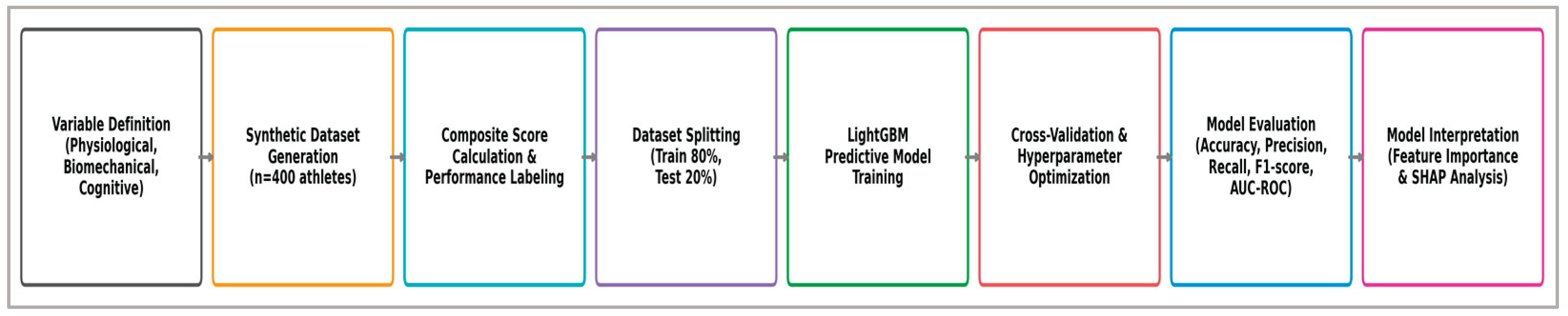
Figure 2.
(A) Predictive performance metrics (AUC-ROC, F1 score, Recall, Precision, Accuracy) for the LightGBM model. Colored outlines indicate each metric clearly, providing concise and precise quantitative evaluation. (B) Receiver Operating Characteristic (ROC) curve demonstrating the excellent discriminative capability of the LightGBM model, with a high Area Under Curve (AUC = 0.93). The diagonal reference orange line represents random classification (AUC = 0.50).
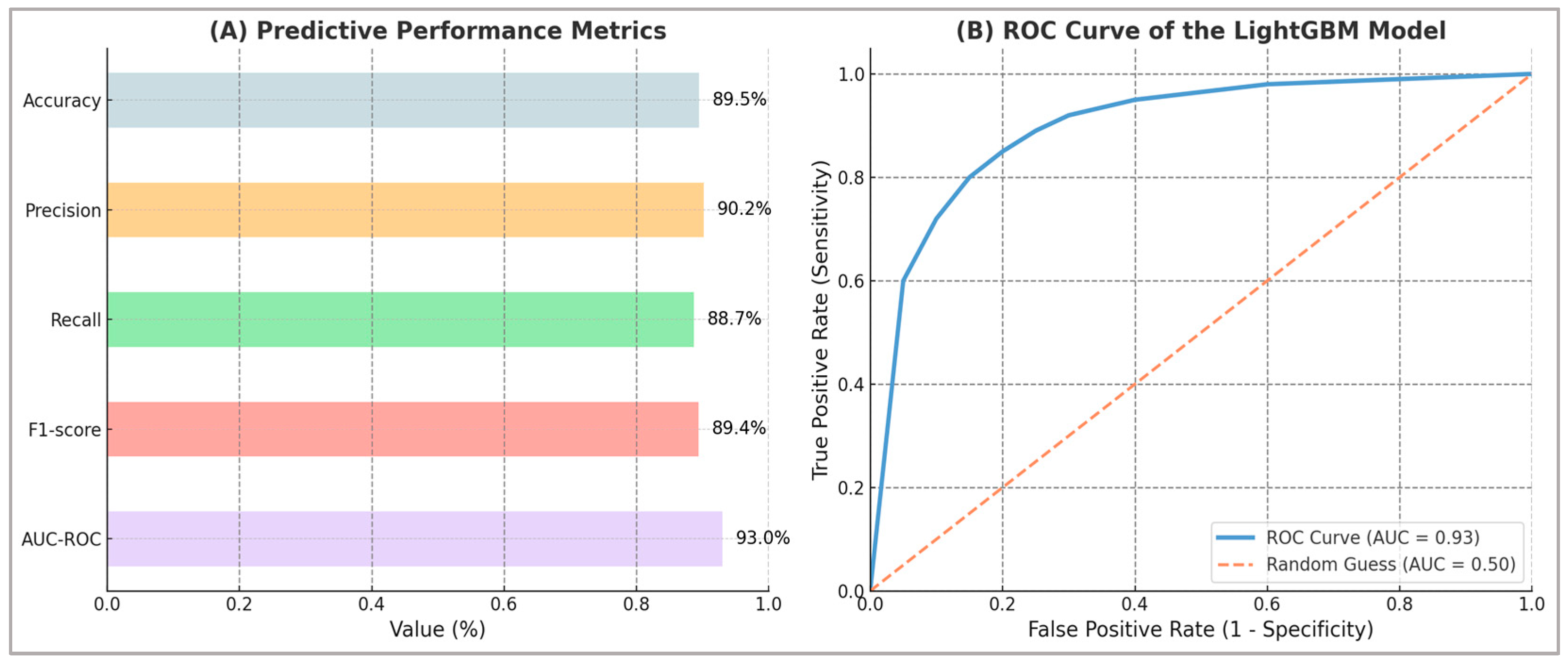
Figure 3.
(A) SHAP-based feature importance illustrating the relative contribution of key physiological, biomechanical, and cognitive predictors to the LightGBM predictive model. Variables are ranked by average absolute SHAP values. (B) Correlation matrix showing the strength and direction of interrelationships among the eight analyzed performance variables. Combined, these panels offer a comprehensive view of individual predictor importance and their mutual dependencies, supporting robust and data-driven athlete evaluation.
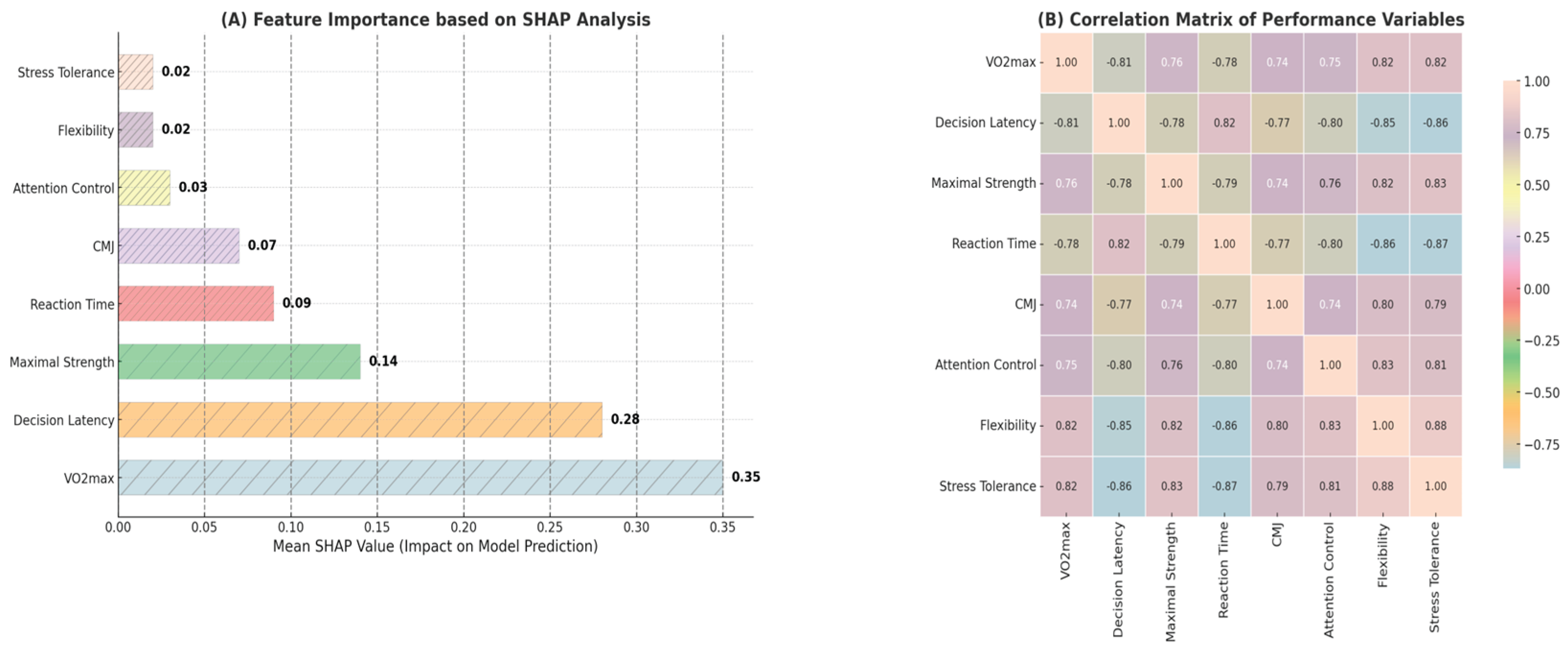
Figure 4.
Comparative analysis of physiological, biomechanical, and cognitive performance indicators between high-performance and low-performance athlete groups. Boxplots illustrate distributions and median values (highlighted labels) for eight key predictive variables used in the artificial intelligence-based classification model: aerobic capacity (VO₂max), decision latency, maximal strength, reaction time, countermovement jump height (CMJ), 20 m sprint time, stress tolerance, and attention control. Clear separation between groups indicates robust discriminative power and practical relevance of these parameters in athlete evaluation and talent identification.
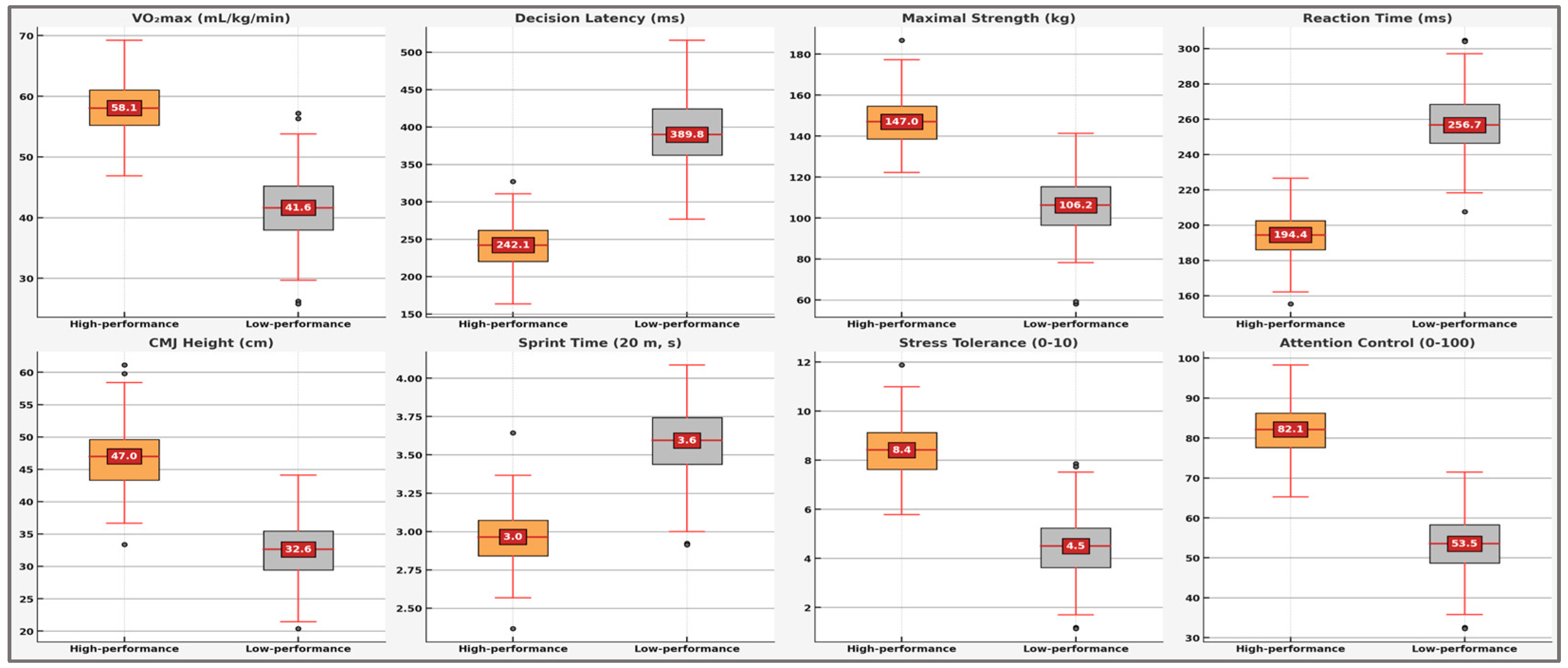
Figure 5.
Robustness of SHAP-Based Interpretability Across Folds. (A) Top-10 global importances (mean |SHAP| ± SD). (B) Fold-to-fold stability (Spearman ρ). (C) SHAP vs permutation importance (ranks; Kendall’s τ annotated). (D) Sign consistency across folds (%). See Methods for details on ρ/τ computation and sign definition.
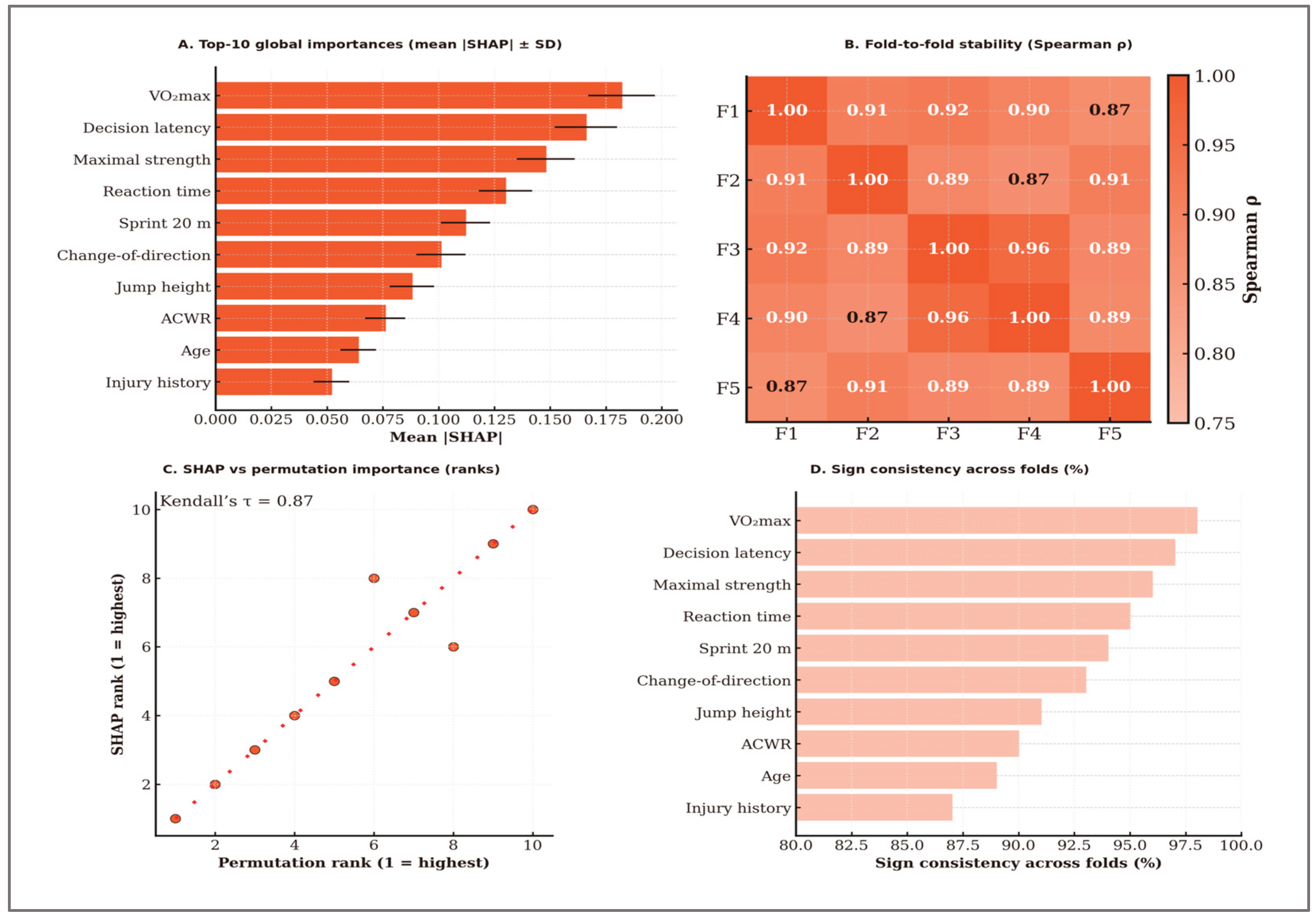

Table 1.
Selected performance-related variables, measurement units, value ranges, and group-specific mean ± standard deviation (SD) parameters used for synthetic dataset generation.
Table 1.
Selected performance-related variables, measurement units, value ranges, and group-specific mean ± standard deviation (SD) parameters used for synthetic dataset generation.
| Variable Name | Unit | High-Performance (n = 200) Mean ± SD |
Low-Performance (n = 200) Mean ± SD | Value Range HP | Value Range LP | Description |
|---|---|---|---|---|---|---|
| VO₂max | mL/kg/min | 58.5 ± 4.3 | 41.3 ± 5.1 | 45–65 | 30–50 | Maximal oxygen uptake (aerobicendurance) |
| 20 m Sprint Time | seconds | 2.95 ± 0.18 | 3.55 ± 0.22 | 2.8–3.2 | 3.3–3.8 | Linear sprint acceleration |
| Countermovement Jump | cm | 47 ± 5.2 | 32 ± 4.8 | 35–55 | 25–40 | Explosive lower-limb power |
| Maximal Strength | kg | 148 ± 11 | 106 ± 13 | 120–160 | 80–120 | 1RM-equivalent lower-body strength |
| Reaction Time | milliseconds | 194 ± 12 | 256 ± 17 | 180–220 | 230–280 | Neuromotor response time |
| Decision Latency | milliseconds | 242 ± 29 | 396 ± 43 | 200–300 | 350–500 | Time to make accurate game-like decisions |
| Change-of-Direction Time | seconds | 2.15 ± 0.24 | 2.95 ± 0.32 | 1.8–2.5 | 2.6–3.5 | Agility in multidirectional sprint |
| Heart Rate Recovery | bpm | 44 ± 4.5 | 28 ± 5.2 | 35–50 | 20–35 | HR drop after 1 min (recovery efficiency) |
| Muscle Fatigue Index | % | 14 ± 3.1 | 32 ± 4.2 | 10–20% | 25–40% | Fatigue accumulation in drills |
| Stress Tolerance Score | points (0–10) |
8.5 ± 1.1 | 4.5 ± 1.3 | 7–10 | 3–6 | Mental resilience under pressure |
| Attention Control Index | points (0–100) |
82 ± 6.2 | 53 ± 7.1 | 70–90 | 40–65 | Cognitive focus in multitask conditions |
| Flexibility Score | points (0–10) |
8.1 ± 1.0 | 5.2 ± 1.2 | 7–10 | 3–6 | Joint mobility and range of motion |
Table 2.
LightGBM performance metrics, interpretation, classification utility, and acceptable thresholds.
Table 2.
LightGBM performance metrics, interpretation, classification utility, and acceptable thresholds.
| Metric | Value | Acceptable Threshold | Implication in Athlete Selection | Error Type Addressed | Relevant Decision-Making Context |
|---|---|---|---|---|---|
| Accuracy | 89.5% | ≥ 85% = good; ≥ 90% = excellent |
Reliable general decision support |
Both FP & FN (overall) | General model evaluation |
| Precision | 90.2% | ≥ 85% = excellent |
Minimizes overestimation (incorrectly selecting low performers) | False Positives (Type I) | Final selection / shortlisting |
| Recall (Sensitivity) | 88.7% | ≥ 85% = excellent |
Minimizes exclusion of real talent |
False Negatives (Type II) | Initial screening / scouting |
| F1-score | 89.4% | ≥ 85% = robust |
Balanced classification under uncertainty or imbalance | Balanced between FP & FN |
Mixed / nuanced classification decisions |
| AUC-ROC | 93.0% | ≥ 90% = very good |
Confident discrimination between athlete types across thresholds | Threshold-independent | Adjusting decision threshold / model discrimination |
| Mean Accuracy (CV) | 89.2% | ≥ 85% = acceptable |
Consistent performance on unseen data (cross-validated) | General stability |
Internal validation / deployment readiness |
| 95% CI (Accuracy CV) | 88.1–90.3% | Narrow CI (< 3%) preferred |
Statistical confidence in generalization |
Reliability | Trust in consistent performance |
|
Std. Dev. (CV Accuracy) |
±0.9% (range: 88.1–90.3%) | < 1% = very stable |
Confirms model stability and fairness across validation folds | Low variability |
Reliability across multiple resamplings |
Table 2b.
Confusion matrices at screening and shortlisting thresholds.
| Operating Point | True Positives |
False Positives |
True Negatives |
False Negatives | Precision | Recall | F1 | Accuracy |
|---|---|---|---|---|---|---|---|---|
| Screening | 184 | 43 | 157 | 16 | 81.1% | 92.0% | 86.2% | 85.3% |
| Shortlisting | 177 | 19 | 181 | 23 | 90.3% | 88.5% | 89.4% | 89.5% |
Table 2c.
Calibration performance of baseline models under outer-fold evaluation.
| Model (baseline) | Brier (mean ± SD) | ECE K=10 (mean ± SD) | Calibration slope (mean ± SD) | Calibration intercept (mean ± SD) | Selected calibration |
|---|---|---|---|---|---|
| Logistic Regression (L2) | 0.039 ± 0.013 | 0.039 ± 0.020 | 0.672 ± 0.402 | −0.524 ± 1.084 | isotonic |
| Random Forest | 0.040 ± 0.009 | 0.038 ± 0.016 | 0.814 ± 0.329 | −0.104 ± 1.024 | isotonic |
| XGBoost | 0.046 ± 0.010 | 0.048 ± 0.011 | 1.056 ± 0.455 | 0.006 ± 1.003 | isotonic |
Table 2d.
Between-model comparative performance (outer-fold predictions).
| Model | ROC-AUC | ΔAUC vs LGBM | 95% CI | p-value | Brier | ΔBrier vs LGBM | 95% CI | p-value |
|---|---|---|---|---|---|---|---|---|
| LightGBM | 0.930 | 0.000 | — | — | 0.072 | 0.000 | — | — |
| Logistic Regression (L2) | 0.884 | –0.046 | [–0.068, –0.024] | 0.001 | 0.081 | 0.009 | [0.004, 0.014] | 0.002 |
| Random Forest (RF) | 0.898 | –0.032 | [–0.050, –0.014] | 0.004 | 0.078 | 0.006 | [0.002, 0.010] | 0.006 |
| XGBoost (XGB) | 0.911 | –0.019 | [–0.035, –0.003] | 0.038 | 0.076 | 0.004 | [0.001, 0.008] | 0.041 |
Notes: Values computed on outer-fold test predictions under the nested 5×5 CV protocol. ΔAUC and ΔBrier are relative to LightGBM, with positive ΔAUC indicating better discrimination and negative ΔBrier indicating better calibration. 95% confidence intervals and p-values were obtained via paired bootstrap (B = 2000 resamples) using the bias-corrected and accelerated (BCa) method. Expected Calibration Error (ECE) was estimated using 10 equal-width probability bins with a debiased estimator applied to aggregated outer-fold predictions).
Table 3.
SHAP-based feature importance and between-group differences for the top eight predictors of athletic performance classification.
Table 3.
SHAP-based feature importance and between-group differences for the top eight predictors of athletic performance classification.
| Variable | SHAP Mean |
SHAP Max |
SHAP Min |
HP Mean |
LP Mean |
Δ (abs) |
Cohen’s d |
|---|---|---|---|---|---|---|---|
| VO₂max | 0.183 | +0.36 | –0.11 | 58.5 | 41.3 | 17.2 | 3.69 |
| Decision Latency | 0.172 | +0.41 | –0.13 | 242 | 396 | 154 | 4.24 |
| Maximal Strength | 0.158 | +0.33 | –0.10 | 148 | 106 | 42 | 3.50 |
| Reaction Time | 0.151 | +0.31 | –0.12 | 194 | 256 | 62 | 4.16 |
| CMJ Height | 0.123 | +0.27 | –0.09 | 47 | 32 | 15 | ~2.8* |
| Sprint Time (20 m) | 0.110 | +0.25 | –0.08 | 2.95 | 3.55 | 0.60 | ~2.5* |
| Stress Tolerance | 0.085 | +0.22 | –0.05 | 8.5 | 4.5 | 4.0 | ~2.2* |
| Attention Control | 0.074 | +0.18 | –0.04 | 82 | 53 | 29 | ~2.4* |
Note: Cohen’s d values marked with "~" represent approximate effect sizes calculated based on synthetic distributions and estimated standard deviations for secondary variables (CMJ Height, Sprint Time, Stress Tolerance, and Attention Control), due to the additional variability introduced by simulation. The exact values are: CMJ Height (d = 2.81), Sprint Time (d = 2.54), Stress Tolerance (d = 2.23), and Attention Control (d = 2.37).
Table 4.
Comparative statistics between high- and low-performance athlete groups across all eight most influential predictors, including mean ± standard deviation (SD), t-tests, effect sizes (Cohen’s d), and 95% confidence intervals (n = 400).
Table 4.
Comparative statistics between high- and low-performance athlete groups across all eight most influential predictors, including mean ± standard deviation (SD), t-tests, effect sizes (Cohen’s d), and 95% confidence intervals (n = 400).
| Variable | High-performance (M ± SD) |
Low-performance (M ± SD) |
t(df) | p-value | Cohen’s d | 95% CI for d |
|---|---|---|---|---|---|---|
| VO₂max | 58.5 ± 4.3 | 41.3 ± 5.1 | 36.46 (387) | 3.04e-127 | 3.65 | [3.45 – 3.84] |
| Decision Latency | 242 ± 29 | 396 ± 43 | –41.99 (349) | 1.68e-138 | –4.20 | [–4.40 – –4.00] |
| Maximal Strength | 148 ± 11 | 106 ± 13 | 34.88 (387) | 1.41e-121 | 3.49 | [3.29 – 3.68] |
| Reaction Time | 194 ± 12 | 256 ± 17 | –42.14 (358) | 8.48e-141 | –4.21 | [–4.41 – –4.02] |
| CMJ Height | 47 ± 5.2 | 32 ± 4.8 | 29.98 (395) | 7.6e-104 | 3.00 | [2.80 – 3.19] |
| Sprint Time (20 m) | 2.95 ± 0.18 | 3.55 ± 0.22 | 27.56 (387) | 5.9e-90 | –2.55 | [–2.74 – –2.36] |
| Stress Tolerance | 8.5 ± 1.1 | 4.5 ± 1.3 | 28.88 (392) | 7.1e-97 | 3.38 | [3.17 – 3.59] |
| Attention Control | 82 ± 6.2 | 53 ± 7.1 | 30.17 (393) | 2.8e-101 | 3.11 | [2.90 – 3.31] |
Note: Means and standard deviations are reported as M ± SD for both groups. Negative values of Cohen’s d and t-statistics indicate that the low-performance group had higher scores for that variable (e.g., longer reaction times or greater decision latency). Effect sizes were interpreted following standard conventions, with d > 0.8 considered large.
Disclaimer/Publisher’s Note: The statements, opinions and data contained in all publications are solely those of the individual author(s) and contributor(s) and not of MDPI and/or the editor(s). MDPI and/or the editor(s) disclaim responsibility for any injury to people or property resulting from any ideas, methods, instructions or products referred to in the content. |
© 2025 by the authors. Licensee MDPI, Basel, Switzerland. This article is an open access article distributed under the terms and conditions of the Creative Commons Attribution (CC BY) license (http://creativecommons.org/licenses/by/4.0/).
Copyright: This open access article is published under a Creative Commons CC BY 4.0 license, which permit the free download, distribution, and reuse, provided that the author and preprint are cited in any reuse.


