Submitted:
18 June 2025
Posted:
19 June 2025
You are already at the latest version
Abstract
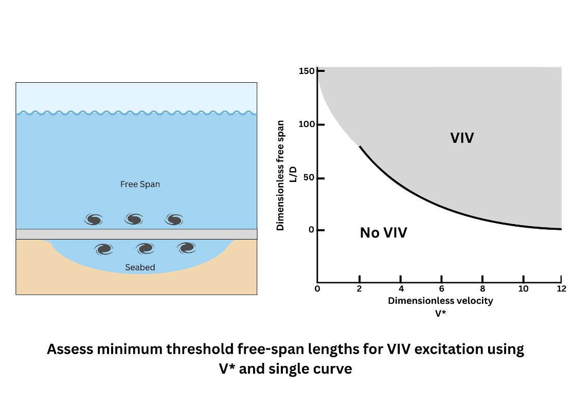
Vortex-induced vibrations (VIV) pose significant risks to the structural integrity of subsea cables and pipelines under free-span conditions. It is extremely helpful to be able to screen for VIV and understand for a particular cable or pipeline what are the minimum free-span threshold lengths beyond which in-line and/or cross-flow VIV can be excited, causing fatigue problems. To date screening is a more complex detailed task. This paper introduces a universal dimensionless velocity, V*, and one graph, that can be used across all types of VIV free spans to quickly assess minimum free-span threshold lengths. Natural frequencies are not required to be calculated for screening each time as they are implicit in the curve. The universal criteria is developed via non-dimensional analysis to establish the significant physical mechanisms, after which the relationships are populated forming a single curve for in-line and for cross-flow VIV with a typical mass ratio and a conservative zero as-laid tension case.
Keywords:
free-span
; viv
; vortex-induced vibration
; pipeline
; cable
1. Introduction
The VIV excitation of free spans pose an integrity concern for subsea power cables, umbilicals, flexible pipes and rigid pipelines.
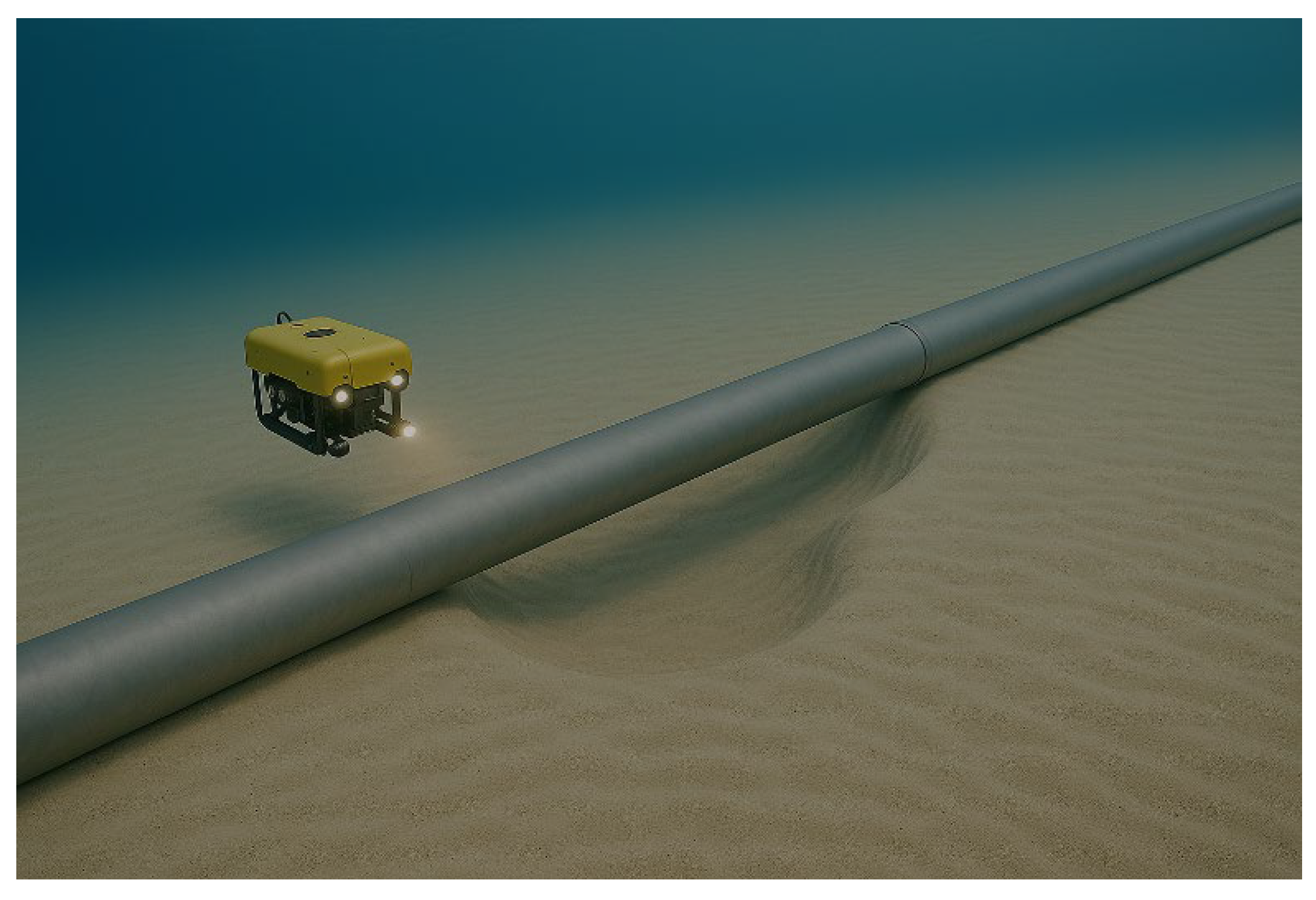
An example power cable VIV free span problem is shown in Figure 1. Free spans can either be present from installation or can grow through seabed changes over time. A good overview of the issues and challenges of free spans is presented in [1], which also discusses advanced analysis techniques. [10] discusses the issues of sag effects in power cables. The relatively complex techniques in [1] and [10] are concerned with evaluating VIV response amplitudes and fatigue lives, whereas this current paper is only concerned with evaluating a screening criteria to determine the necessary conditions for the onset of VIV.
In order to assess fatigue lives of free spans, one can turn to industry codes of practice [2] and analysis tools such as SHEAR7 [3] and FATFREE [4]. These methods provide response predictions and can be used to compute estimated fatigue damage. Prior to undertaking response predictions, it would be useful to have an expedient screening tool for free spans. Up until now, there has not been a universal screening criteria that allows a simple one step check.
The Onset of VIV
A free span subject to a monotonically increasing current will generally experience the onset of in-line VIV prior to the onset of cross-flow VIV. This is because vortex shedding causes two in-line direction cycles of excitation for every one cross-flow cycle of excitation.
The onset of VIV is typically assessed by the coinciding of an excitation frequency with a natural frequency (including tolerance, or bandwidth). Typically for fatigue sensitive structures an operating philosophy can involve avoiding in-line VIV altogether by keeping the excitation frequency always lower than the first response (natural) frequency. This can become challenging as the natural frequency gets lower with increasing span lengths.
To make the comparison of the natural frequencies and excitation frequencies from the current or wave induced current action, existing pre-screening checks require calculation of the natural frequency each time a structure and different span length is measured. A more efficient method would eliminate the need to compute the natural frequency all together.
2. Non-Dimensional Analysis
Identification of Relevant Variables and Dimensions
A non-dimensional analysis can reveal governing physics and highlight which physical effects dominate a system. The Buckingham Pi theorem [5] is utilized to perform a nondimensional analysis on a typical VIV free span problem.
Firstly, all physical variables influencing the problem are listed, along with their dimensions, which in this problem are confined to Mass [M], Length [L] and Time [T]:
- Characteristic outside diameter D [L]
- Current velocity, V [LT−1]
- Fluid density ρf [ML−3]
- Mass density of structure (cable or pipe) ρS [ML−3]
- Characteristic free span length, L [L]
- Cable or pipe bending stiffness, EI [MLT−2.L2 = ML3T-2]
- Cable or pipe as-laid effective tension, Teff [MLT−2]
Summarizing the list or physical variables: D, V, ρf, ρS, L, EI, Teff.
The above list gives n = 7 parameters. Per the Buckingham Pi theorem, the independent dimensions are defined for this problem as being confined to M, L and T. Hence the total independent dimensions, m, is m = 3.
The number of Nondimensional Groups is calculated by the Buckingham Pi theorem as n – m = (7) – (3) = 4.
The non-dimensional groups are now constructed by choosing convenient repeating variables (any can be chosen, but the choices are made to gain greater physical interpretation of the groups). These are provided with a physical interpretation in paratheses as:
- D (geometric),
- V (kinematic), and
- ρf (dynamic).
These repeating variables are used to solve and represent each of the remaining group’s expressions.
The remaining groups, Π, are now solved and physical interpretations are included in paratheses after each group:
For Mass density of cable or pipe, ρs,
Π1 = ρs . Da . (ρf)b . Vc
Π1 = (ML−3) . [L]a . (ML−3)b . [LT−1]c
Π1 = M1+b L-3+a-3b+c T-c
Equating exponents:
1+b=0 -> b=-1
-c=0 -> c=0
-3+a-3b+c=0 -> a=0
Π1 is commonly called the specific gravity, or m*, the mass ratio, although some historical definitions of mass ratio differ by a factor of in the denominator [6].
For span length L,
Π2 = L . Da . (ρf)b . Vc
Π2 = L . [L]a . (ML-3)b . [LT−1]c
Π2 = Mb L1+a-3b-c T-c
Equating exponents
-3b=0-> b=0
-c=0-> c=0
1+a-3b+c=0 -> a=-1
L/D is commonly referred to as the aspect ratio.
For EI,
Π3 = EI . Da . (ρf )b . Vc
Π3 = ML3 T-2 . Da . (ρf)b . Vc
Π3 = (ML3 T-2) . [L]a . (ML−3)b . [LT−1]c
Π3 = M1+b L3+a-3b+c T-2-c
Equating exponents
1+b=0 -> b=-1
-2-c=0 -> c=-2
3+a-3b+c=0 -> 3+a-3(-1)+(-2)=0 -> a=-3-3+2=-4
Π3 = EI . D-4 . (ρf)-1 . V-2 or:
EI represents (flexural) bending stiffness. represents a fluid induced forcing moment. The ratio represented in Equation 3 therefore is a flexural stiffness ratio, comparing structural resistance to fluid-induced forcing moment.
For convenience, it becomes easier to use as a velocity term as engineers are often dealing with velocity as an input term for span analysis problems. Accordingly, the expression is changed the expression by inversion, inclusion of a square root and multiplying by 1000 (none of those operations changes the fact that it is still a dimensionless expression). The resulting expression is chosen here to be named V*, a dimensionless velocity number as shown in Equation 4. This can be expressed for either in-line or cross-flow, VIL* or VCF* (with corresponding VIL or VCF - the dimensional onset velocities for VIV).
For Teff,
Π4 = Teff . Da . (ρf)b . Vc
Π4 = MLT−2 . Da . (ρf)b . Vc
Π4 = (MLT−2) . [L]a . (ML−3)b . [LT−1]c
Π4 = M1+b L1+a-3b+c T-2-c
Equating exponents
1+b=0 -> b=-1
-2-c=0 -> c=-2
1+a-3b+c=0 -> 1+a3(-1)+(-2) -> 1+a+3-2 => a=-2
Π4 = Teff . D-2 . (ρf )-1 . V-2. or:
represents a dynamic pressure, with the multiplication of D2 it becomes a fluid induced force. T is the axial tension (a force). represents the relative loading from tension versus fluid force. More relationships can be explored with if one is interested in non-zero as-laid tensions of cables and pipelines. For the purposes of screening, we can assume zero as-laid tension which will under-predict natural frequency values and therefore conservatively predict the onset of VIV at lower velocities than would occur with non-zero as-laid tension cases.
Simplified Governing Equations
The original system reduces to be described by Equation 6. Note that for completeness the dimensionless parameter Strouhal number, St, is introduced here:
This expression can be simplified, by ignoring tension effects to Equation 7:
The non-dimensional analysis has revealed the commonly held knowledge that predicting VIV free spans are a function of mass ratio and aspect ratio. If St is assumed constant, then Equation 7 reduces to Equation 8 as a three-parameter simplification:
3. Simplified Response Curve
With only three parameters, two parameters can be plotted against one another for various values of the third parameter. Accordingly, L/D vs V*, a normalised span length versus a dimensionless velocity, is chosen for various m* values.
We can now simplify the problem, by assuming a typical mass ratio, to predict the onset of VIV to one universal curve for in-line VIV and one for cross-flow VIV.
Whilst various assumptions can be made to construct the curve, it is convenient to align the assumptions with DNV assumption for ease of agreement with the RP [2]. The curve is constructed using the following assumptions for in-line VIV:
- Clamped-clamped end condition (per DNV [2] single span recommendation)
- Ca = 1.0
- Safety factor on onset value for in-line, γonIL = 1.1; (cross-flow onset safety factor not applied in determining cross-flow VIV onset condition in [2] )
- Safety factor on in-line and cross-flow natural frequencies, γ fIL = 1, γ fCF = 1
- Lowest natural frequencies in in-line and cross-flow directions for a given span are termed fIL,1 and fCF,1 and computed per Section 2.2 in [2]
- VR onset for cross-flow VIV is effectively 2.0 (Section 2.3.3 [2])
- No multi-spans, interactions between spans or significant sagging is considered
- This covers screening for fatigue (FLS), not local buckling of ultimate stress (ULS)
A clamped-clamped transverse pipe 1st natural frequency (from [2,7]) is shown in Equation 9, with rearrangement of this in terms of L (or Leff from [2]) as shown in Equation 10.
EI is the bending stiffness, me the mass per unit length including structure, contents and added mass, L is the length of the span in this scenario.
A plot of L/D vs V* for IL and CF, with a typical value of mass ratio (m* = 3) assumed, is shown in Figure 2. These plots represent universal free span thresholds to predict the onset of VIV. Left of each respective curves is No-VIV predicted, right of each respective curve is a potential VIV excitation condition.
Table 2. can be represented by the following equations, within the bounds of exploration, Equations 11a/b for in-line and Equation 12a/b for cross-flow:.
A more detailed plot of in-line VIV onset (L/D)IL vs V* and cross-flow VIV onset (L/D)CF vs V* for some typical values of mass ratios are shown in Figure 3 and Figure 4 respectively. The graphs show that for screening purposes, values for m* = 3 are a reasonable assumption, if the mass ratio is within ~ +/- 0.5 of 3.0.
4. Case Studies
Power Cable Free Span Screening – Minimum Velocity
A power cable free span case study (as illustrated in Figure 1) with a known free-span length, is assessed to determine the critical minimum velocities for the onset of in-line and cross-flow VIV. The cable properties are largely taken from Table 1 of [8].
Analysis Parameters
Inputs:
- Free-span length, L = 5 m
- Diameter, D = 0.176 m
- Bending Stiffness, EI = 12 kN·m²
- Mass/Length = 77.3 kg/m (
Outputs:
- L/D = 28, m* ~ 3 (from Equation 1) (as ~3, use Figure 1)
- VIL* ~ 2.8, VCF* ~ 5.9 (from Fig 2)
- Onset velocities VIL ~ 0.3 m/s, VCF ~ 0.65 m/s (from Equation 4)
Pipeline Free Span screening – Maximum Span Length
A pipeline free span case study (illustrated in Figure 5) is shown below to assess the inverse problem – determining what is the critical minimum span length for the onset of VIV with a known maximum velocity. The pipeline properties are hypothetical.
Analysis Parameters
Inputs:
- Diameter, D = 0.483 m (19 inch)
- Maximum V: 1.7 m/s
- Bending Stiffness, EI: 4.68e7 N·m²
- Mass/Length = 518 kg/m
Outputs:
- m* = 2.8 (from Equation 1) (as ~3, use Figure 1)
- V* = 1.85 (from Equation 4)
- Critical minimum span lengths: (L/D)IL = 34, (L/D)CF = 50, ∴LIL = 16 m, LCF = 24 m
5. Discussion
If VIV is found to be potentially excited, then higher fidelity calculations are advisable including fatigue predictions for the expected current profiles with their associated probabilities of exposures. Fatigue is generally assessed using industry codes such as DNV [2] or analysis tools such as SHEAR7 [3].
If predicted fatigue live is found to be less than project life, including the appropriate safety factors, there are many VIV treatment options widely used in industry. If the system is already in place, then post installation of hydrodynamic shrouds can be performed. Such shrouds include Longitudinal Grooved Suppression (LGS) [9], or helical strakes if clearance to seabed permits. These treatment options each have their own benefits and disadvantages. Where the LGS solution provides less reduction in VIV compared to helical strakes, it is less confined geometrically as a post-installed solution. The LGS treatment also grants a significant decrease in static drag of the free span, compared to an increase in drag seen by the straked solution. Increase in drag can create issues if the cable/ pipeline is adjacent to other subsea infrastructure where potential clashing is possible.
More expensive alternate options likely involve changes to the foundation via support additions [1] or even rock dumping. Although more expensive this has the benefit of reducing or eliminating the free span entirely or significantly reducing the effective free span length, thus preventing fatigue accumulation to undesirable levels.
If the system is not already installed additional options may be to investigate changing the routing of the pipeline / cable to avoid potential spanning scenarios where fatigue damage will be an issue. However, this may result in additional time and expense due to lengthening of the required pipeline / cable for both installation and manufacturing.
The observations seen in this paper and relationship between onset velocity for VIV and free span length is limited to when the Strouhal number and tension variation is held constant. In scenarios of free span where this is not the case, the reader should apply a similar non-dimensional analysis approach to consider the effects of these changes.
6. Conclusions
As a result of the non-dimensional assessment of VIV onset when applied to free spans outlined in this paper the following conclusions can be drawn regarding creating a universal screening criteria:
- The non-dimensionalisation of a free span under VIV revealed three dominant physical mechanisms, mass ratio, aspect ratio and bending stiffness curvature loading.
- The mass ratio within the range investigated does not show significant influence on the critical free span length for a given non-dimensional flow velocity.
Abbreviations
The following abbreviations are used in this manuscript:
| CF | Cross-Flow |
| IL | Inline |
| LGS | Longitudinal Grooved Suppression |
| VIV | Vortex Induced Vibration |
Data Sharing
Data sharing is not applicable (only appropriate if no new data is generated or the article describes entirely theoretical research).
References
- Martins, R.R.; Cardoso, C.O.; Matt, C.G.C.; Nunes, L.A.N.; Góes, R.C.O.; Rosa, A.S.; Silveira, E.S.S. Improving the Free Span Analysis of Subsea Rigid Pipelines for Life Extension Through Integration and Automation and Efficiency. In Proceedings of the Offshore Technology Conference; OTC: Houston, Texas, USA, April 28 2025; p. D021S022R008.
- Free spanning pipelines. DNV-GL-RP-F105. Edition 2017-06 - Amended 2021-09. Recommended Practice.
- shear7.com accessed 10 June 2025.
- https://sesam.dnv.com/download/userdocumentation/fatfree-user-manual.pdf accessed 10 June 2025.
- Kelly, S.G. Fundamentals of Mechanical Vibrations; McGraw-Hill series in mechanical engineering; McGraw-Hill: New York, 1993; ISBN 978-0-07-911533-1. [Google Scholar]
- Vandiver, J.K. Dimensionless Parameters Important to the Prediction of Vortex-Induced Vibration of Long, Flexible Cylinders in Ocean Currents. Journal of Fluids and Structures 1993, 7, 423–455. [Google Scholar] [CrossRef]
- Rao, S.S. Mechanical Vibrations; Sixth edition.; Pearson: Hoboken, NJ London Toronto, 2017; ISBN 978-0-13-436130-7. [Google Scholar]
- https://www.nrel.gov/docs/fy21osti/76968.pdf accessed 10 June 2025.
- Jayasinghe, K.; Marcollo, H.; Potts, A.E.; Dillon-Gibbons, C.; Kurts, P.; Pezet, P. Mitigation of Pipeline Free Span Fatigue Due to Vortex Induced Vibration Using Longitudinally Grooved Suppression. In Proceedings of the Volume 5: Pipelines, Risers, and Subsea Systems; American Society of Mechanical Engineers: Madrid, Spain, June 17 2018.
- Zhu, J.; Ren, B.; Dong, P.; Chen, W. Vortex-Induced Vibrations of a Free Spanning Submarine Power Cable. Ocean Engineering 2023, 272, 113792. [Google Scholar] [CrossRef]
Figure 1.
A power cable free span that can be subject to currents and undergo VIV (AI generated illustration).
Figure 1.
A power cable free span that can be subject to currents and undergo VIV (AI generated illustration).
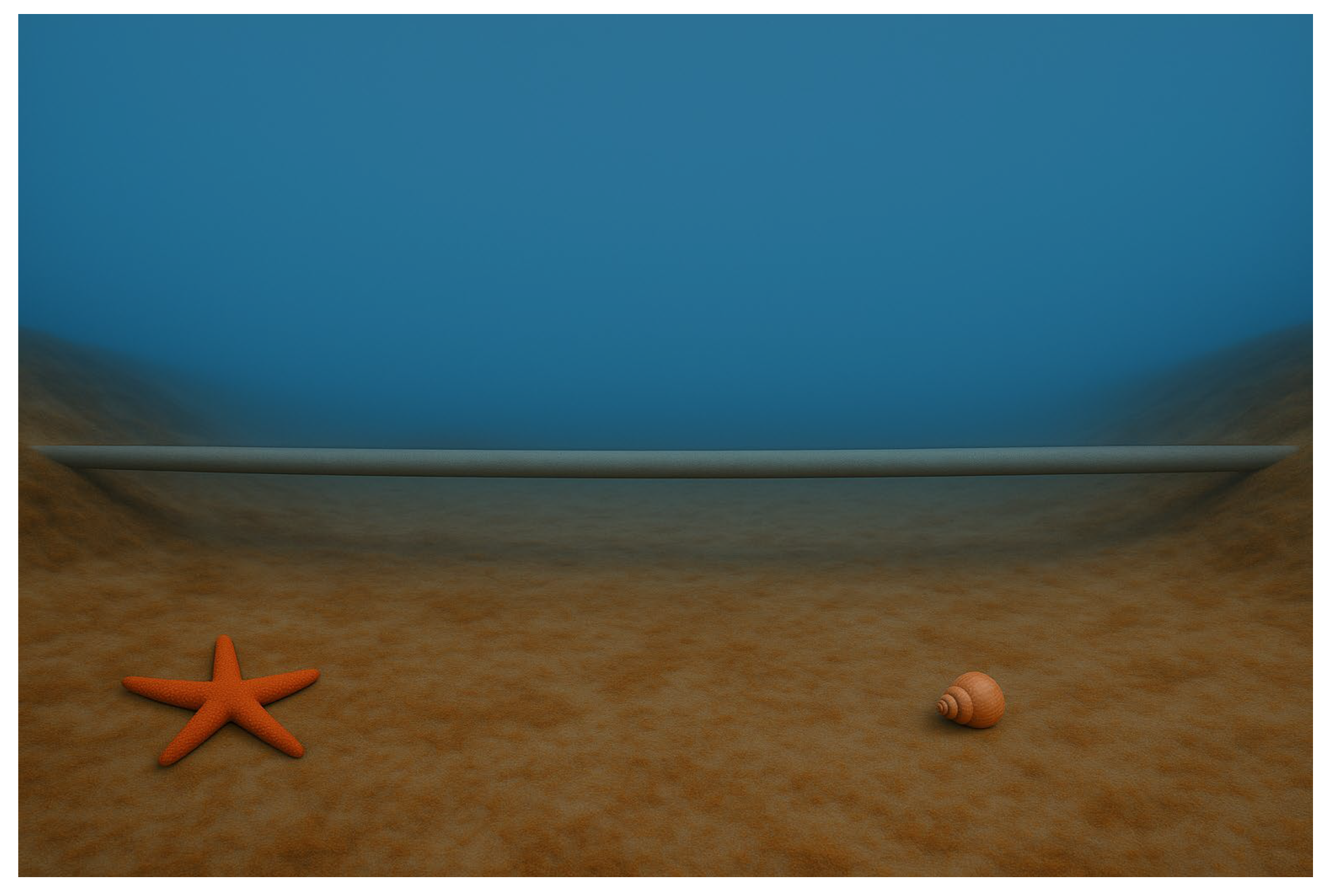
Figure 2.
Dimensionless universal free span threshold relationships for typical mass ratio, m* = 3. V* is defined in Equation 4. Left of each respective curve is No-VIV, right is a potential VIV.
Figure 2.
Dimensionless universal free span threshold relationships for typical mass ratio, m* = 3. V* is defined in Equation 4. Left of each respective curve is No-VIV, right is a potential VIV.
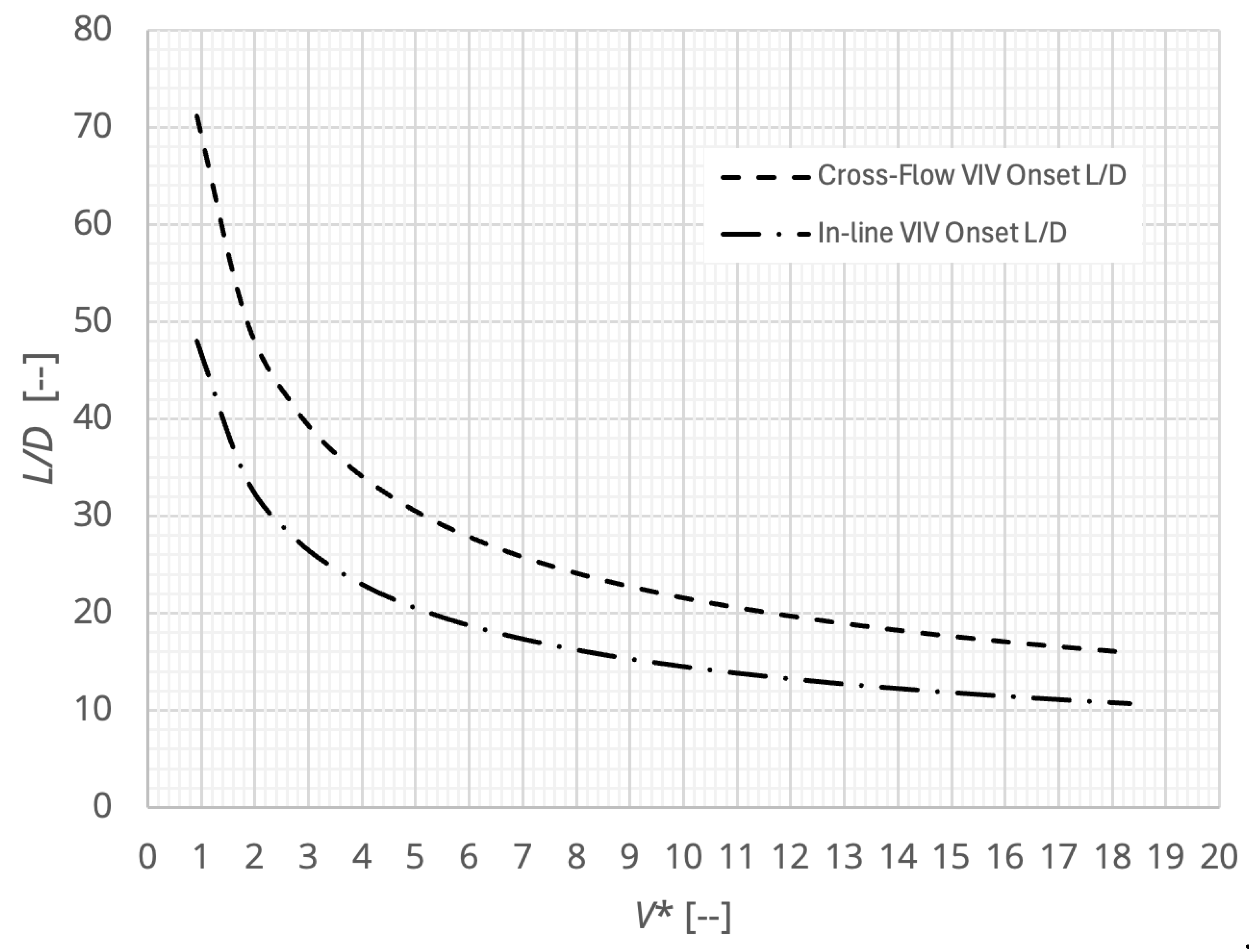
Figure 3.
In-line VIV onset (L/D)IL vs V* for a range of mass ratio values. V* is defined in Equation 4.
Figure 3.
In-line VIV onset (L/D)IL vs V* for a range of mass ratio values. V* is defined in Equation 4.
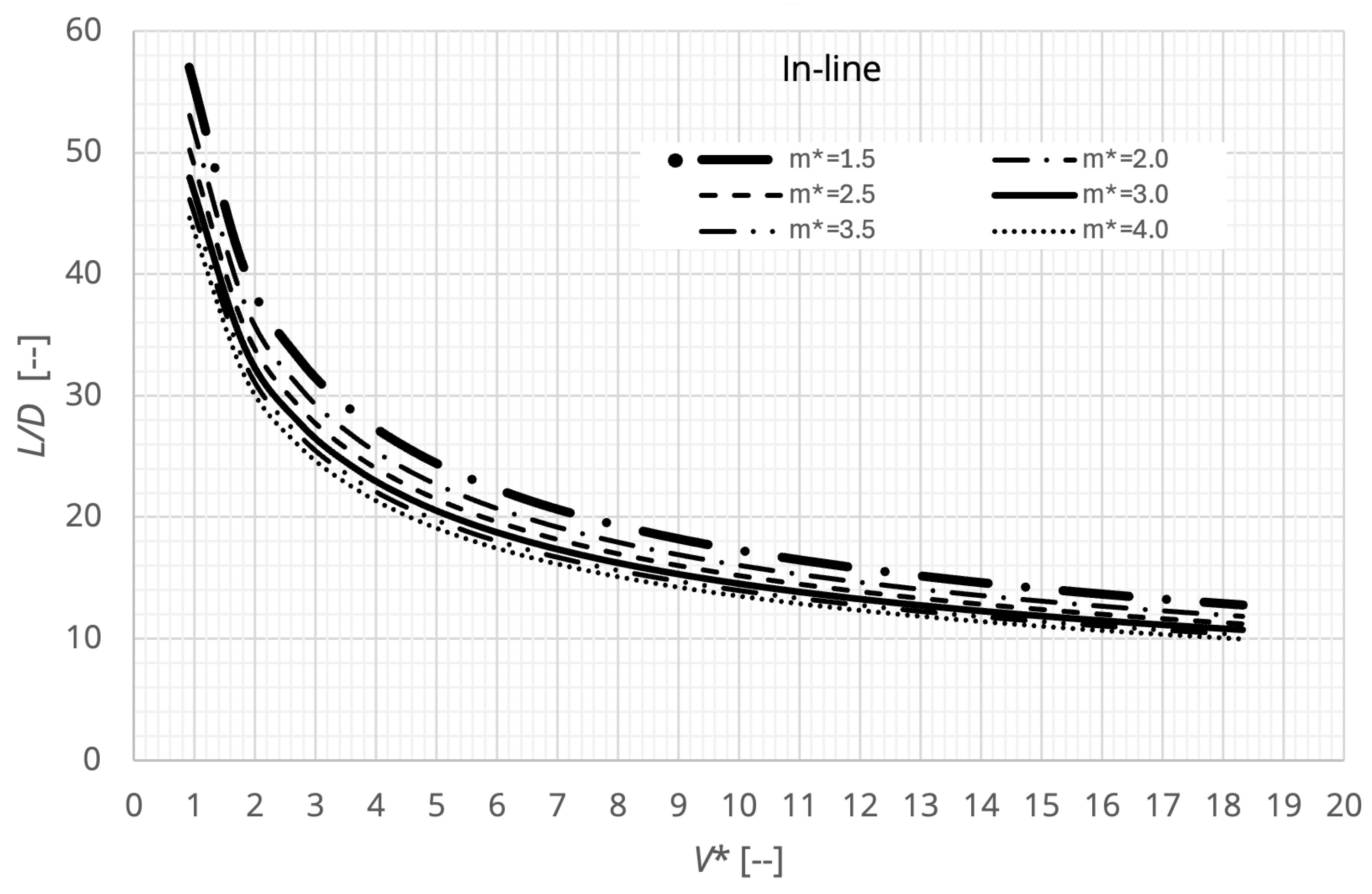
Figure 4.
Cross-flow VIV onset (L/D)CF vs V* for a range of mass ratio values. V* is defined in Equation 4.
Figure 4.
Cross-flow VIV onset (L/D)CF vs V* for a range of mass ratio values. V* is defined in Equation 4.
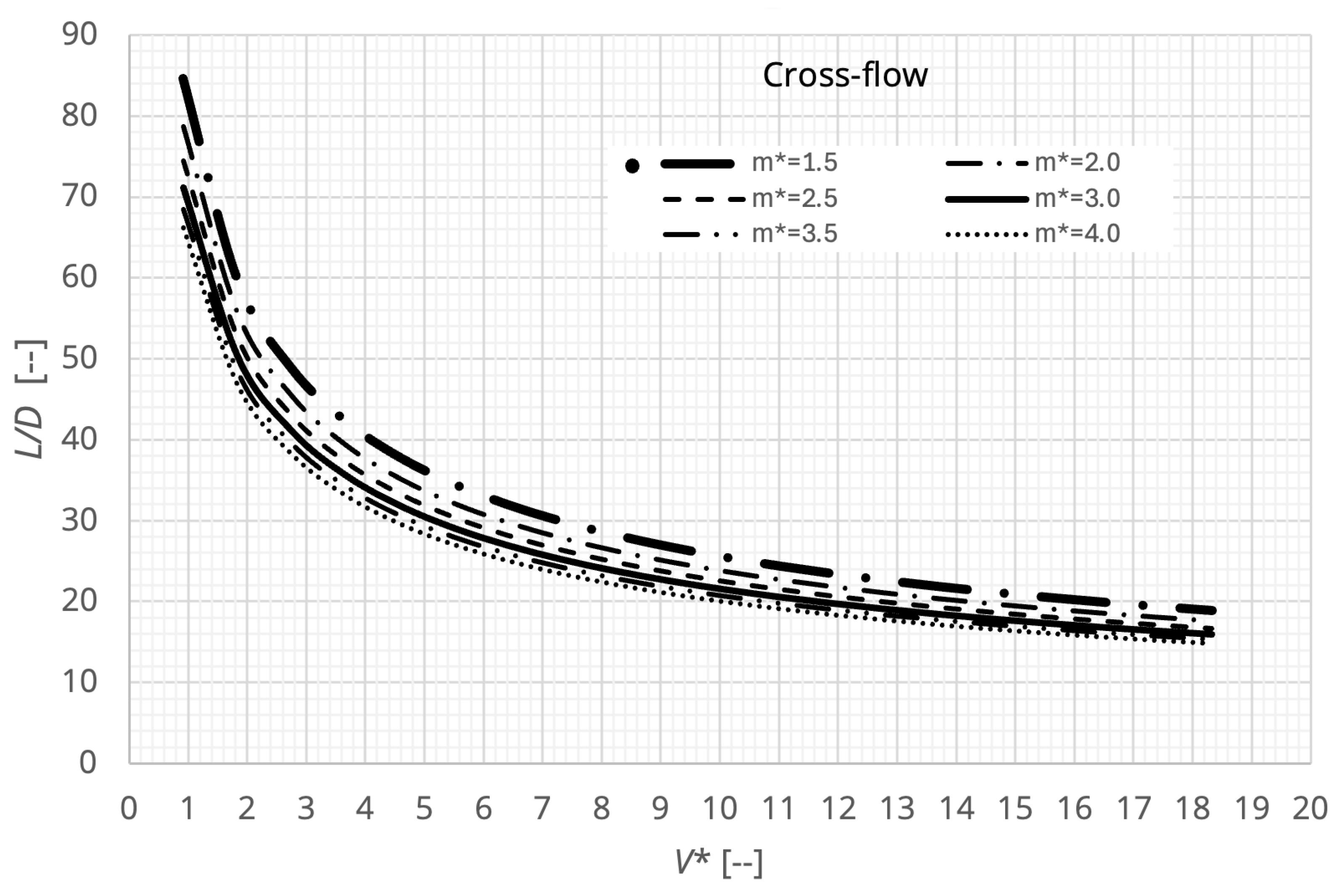
Figure 5.
VIV free span growing over time with sand erosion (AI generated illustration).
Disclaimer/Publisher’s Note: The statements, opinions and data contained in all publications are solely those of the individual author(s) and contributor(s) and not of MDPI and/or the editor(s). MDPI and/or the editor(s) disclaim responsibility for any injury to people or property resulting from any ideas, methods, instructions or products referred to in the content. |
© 2025 by the authors. Licensee MDPI, Basel, Switzerland. This article is an open access article distributed under the terms and conditions of the Creative Commons Attribution (CC BY) license (http://creativecommons.org/licenses/by/4.0/).
Copyright: This open access article is published under a Creative Commons CC BY 4.0 license, which permit the free download, distribution, and reuse, provided that the author and preprint are cited in any reuse.


