
Submitted:
12 June 2025
Posted:
16 June 2025
You are already at the latest version
Abstract
This work examines dynamic models for describing the viscoelastic behaviour of short-fibre reinforced plastics in tensile tests. The creep behaviour of reinforced PBT GF30 compared to unreinforced PBT GF0 is investigated on the basis of experimental data. Two different modelling approaches are compared: a generalised Maxwell model based on the prony series and a model with fractional derivatives. The experimental data show that glass fibres significantly reduce the deformation under constant load, as they stiffen the polymer matrix and inhibit creep deformation. Parameters can be determined for both models using machine learning methods. However, the Prony-Maxwell based model requires three parameters to accurately represent the data, whereas the fractional model only requires two parameters. The results clearly show the advantages of fractional model for the description of the long time series behaviour: on the one hand, fewer parameters are required and on the other hand, additional knowledge can be gained through the interpretation of the parameters obtained. The experimental data as well a the open-source software developed to learn the model is published alongside this work.
Keywords:
short fiber-reinforced composite
; viscoelasticity
; FDE solver
; Prony series
; fractional derivative
; tensile creep test
1. Introduction
Short Fibre-Reinforced Composites (SFRCs) are widely used in various engineering fields like aerospace and automotive industries. Their mechanical properties including high stiffness and strength, together with their suitability for cheap, large-scale automated production recently increased the interest in SFRC [1,2,3,4,5,6].
SFRC materials consist of two or more different materials that are combined during a mold injection process [7,8]. While thermoplastic Polybutylene Terephthalate (PBT) is serving as matrix material, the short glass fibres reinforce the structure leading to increased stiffness and strength. However, polymer-based composites, such as PBT GF30, show time-dependent deformation when subjected to sustained loads, which is commonly referred to as viscoelasticity or creep. Typically creep is caused by the matrix material [9,10,11]. To predict the long-term performance of components, it is important to accurately characterise the creep behaviour, especially for the automotive, aerospace, and electronics industries [1,2,3,4,5].
Viscoelastic behaviour of SFRC is typically described using the generalised Maxwell model [12], which combines springs and dampers to represent elastic and viscous elements [12,13]. The Maxwell model is standardised and widely used in commercial Finite Element Method (FEM) software packages [14,15]. Its implementation in FEM relies on the Prony series [12,16,17], where the Prony series reflect the solution of an Ordinary Differential Equation (ODE), which results from the combination of springs and dampers. As these elements are typically considers to be linear, the ODE solution can be modelled as a sum of exponential functions. The effectiveness of this approach requires a large number of parameters to capture the full spectrum of material behaviour on varying time scales. This increases the complexity of parameter identification as well as computational cost [16,17,18].
While Prony based models approximate the non-local nature of creep effects by superposition of several spring and damper elements, fractional derivate models inherently can model this behaviour. A fractional derivate model, also referred as fractional element, describes dynamics that lie between a spring and a damper [12,19,20]. However, practical application of fractional models remain challenging: Normally these models are solved indirectly by transforming them into the Fourier domain to fit experimental data. While established, this approach requires more complex data collection setups as the material behaviour has to be measured across different frequencies in the frequency domain. This makes simple tensile tests insufficient for data collection. Furthermore, Fourier analysis is limited to linear models, which complicates the representation of non-linear behaviour [21,22].
Recent advances in machine learning (ML) have enabled to learn fractional dynamics directly from data. Coelho et al. [23] introduced Neural Fractional Differential Equations (NFDEs). NFDEs combine a solver for Fractional Dynamical Equations (FDEs) with Neural Nets (NN) to learn the underlying FDE from arbitrary data. Building on this foundation, Zimmering et al. [24] improved the solver in accuracy and resource efficiency, enabling to use the solver in real-world scenarios
In this study we overcome the need for special experiments that capture the frequency spectrum of SFRC to fit a fractional element model. We utilize the optimised NFDE solver of Zimmering et al. to fit parametric fractional models directly to experimental data from tensile tests. The solver’s general capability to fit arbitrary dynamical models (including NNs) additionally offers flexibility in capturing non-linear creep behaviour from arbitrary data in future studies.
Following this, our contributions are:
- First we compare the accuracy of fractional element in describing the creep behaviour of PBT GF0 and PBT GF30 with the generalized Maxwell model. This comparison aims to determine the to which extend fractional derivative models can effectively capture the viscoelastic response of such materials over time.
- Second we study practical methodologies to efficiently learn the parameters of fractional element models. We seek to identify computational techniques that enable a stable parameter identification process while maintaining accuracy.
- Third we discuss the advantages that fractional derivative models may offer over the Prony models for SFRC. We evaluate if fractional models provide improved predictive capabilities and enhance representation and interpretability of material properties over extended time scales.
This paper is structured as follows: Section 2 outlines the theoretical framework for modelling creep behaviour as well as the data fitting methods for the Prony fractional model. Section 3 details the experimental setup for the data acquisition methods. In Section 4 the results are presented. Here we focus on the determination of Prony coefficients and coefficients derived from fractional models. Finally, in Section 5, we discuss the comparative performance of the models and draw conclusions about their practical applications in material characterization.
The developed software is based on Python and open-source software libraries and available along with the experimental data at https://github.com/zimmer-ing/PBTGF-Creep. This allows others to reproduce the results, apply the presented methods in their own work.
2. Materials & Methods
2.1. Theoretical Framework for Creep Behavior
Creep is a time-dependent deformation process that occurs under constant load and temperature, involving both elastic and viscous contributions. This phenomenon is particularly relevant in polymer-based materials, which exhibit viscoelastic behaviour, which combines time-independent elasticity and time-dependent viscous flow.
2.1.1. Viscoelastic Effect
Creep occurs when a material undergoes time-dependent deformation under constant load and temperature. This effect occurs in polymer-based materials, which has both elastic and viscous behaviour, commonly referred to as viscoelastic behaviour [12,17,25,26]. In general, creep deformation typically occurs in three stages: primary, secondary, and tertiary creep, as illustrated in Figure 1, where the strain over time t is shown schematically.
The primary creep stage is characterised by a deceleration in the strain rate. It occurs immediately after stress application, with the initial strain representing the elastic response [27]. The secondary creep stage is marked by a constant strain rate and is crucial to evaluating long-term material behaviour. It is typically the longest stage. In the tertiary creep stage, the strain accelerates rapidly until material failure.
The total strain over time of the sample under constant loads, as schematically presented in Figure 1, can be expressed additively as
Here, represents the immediate strain response upon the application of stress, following Hooke’s law for linear elasticity. This component remains constant over time and does not contribute to the time-dependent deformation behaviour of the material. However, the creep deformation accounts for the viscoelastic deformation that evolves over time under sustained loading including all three stages. In this work, the focus is on the primary and secondary stages, because capturing the tertiary stage is time consuming and experimentally challenging.
In addition to creep, viscoelastic materials show relaxation behaviour, which is another fundamental time-dependent property. Relaxation occurs under conditions of constant strain, where the initial applied stress decreases over time as the material redistributes internal stresses to balance its elastic and viscous components. Stress relaxation provides crucial insights into the ability of the material to maintain integrity under sustained deformation[12,25].
The mathematical models are derived using rheological elements that describe the stress-strain relations for the linear viscoelastic behaviour [12,28]. These elements are shown in Figure 2, where the spring element represents Hooke’s law with stiffness . A dashpot represents a purely viscous material according to Newton’s law characterised with dynamic viscosity . The fractional element is described by parameters C and .
Generally, there are two equivalent approaches to characterise the mathematical relationships between stress and deformation in linear viscoelastic materials [12,17,25,26,27]. One approach employs integral formulations to establish these relationships, while the other uses first-order ODE to connect stresses and strains. The integral formulation is where Boltzmann first articulated the superposition principle, commonly referred to as the Boltzmann superposition principle [12,29]. This integral formulation for linear viscoelastic materials describes the response to strain as a function of past stresses and a function of material stiffness. It is written as [12]
where represents the creep stiffness. If the roles of stress and strain are reversed, Equation (2) can be rewritten as
where denotes the creep compliance. Equation (2) can be read as follows: The strain at the specific time t is composed of all past stresses , multiplied by the corresponding stiffness , known as material function. The time interval measures the duration since the stress was applied. The material function depends on the material and can be obtained experimentally. The corresponding differential equations for viscoelastic materials will be introduced in the next section. In the context of experimentally measured creep data, the creep stiffness can be determined as follow
where is the sustained load, and gives the measured time-dependent creep elongation.
2.1.2. Generalized Maxwell Model and Prony-Series
The basic Maxwell model, shown in Figure 3 a), consists of a spring and a dashpot connected in series. This approach is able to represent simple viscoelastic behaviour, however it cannot fully capture the complex time-dependent response of materials. To overcome this limitation, multiple Maxwell models are arranged in parallel with an additional spring , as shown in Figure 3b). This extended configuration is known as the generalized Maxwell model [17,30,31]. This model is able to capture the viscoelastic properties of materials, including their memory effects and time-dependent creep behaviour. Each individual Maxwell element is governed by a first-order ODE [17,31].
The total stress is modelled as the sum of the contributions of the Maxwell elements N, each representing a viscoelastic branch of the material. The constitutive behaviour of the i -th Maxwell element is governed by a first-order differential equation that relates stress and strain through elastic and viscous parameters. The governing equation for the i -th branch is given by [30,32]
where represents the stress contribution of the i-th Maxwell element, is the elastic modulus of the i-th spring, and is the relaxation time of the i -th Maxwell element, defined as , with being the viscosity of the dashpot. The initial condition for each Maxwell element is given by , indicating the initial stress in the element, while the initial strain is generally assumed to be zero , in creep experiments. The total stress is expressed as the sum of the stresses of all the i-th Maxwell elements
where are fitting coefficients representing the contribution of each Maxwell element [31]. This formulation is known as the Prony-series [12,31].
For the generalized Maxwell model, as detailed in [12,17,25,31,32,33], the stress-strain relationship for viscoelastic materials in the form of a differential equation is formulated as follows
This differential equation (7) effectively models the viscoelastic response of complex materials, encompassing both stress relaxation and creep behaviour [32].
A widely used approach to describe the time-dependent viscoelastic response is the Prony series, which can be derived by applying the Laplace transform to the differential formulation of the generalized Maxwell model, such as Equation 7 [12]. The Prony series allows for precise fitting to experimental data by expressing the material stiffness as a sum of exponential terms, each representing a Maxwell element with a specific relaxation time and modulus. The Prony series effectively describes the time-dependent deformation behaviour of materials, which is written as [12]
The relaxation function characterises the time-dependent decrease in material stiffness due to viscoelastic effects. Each exponential term corresponds to a Maxwell element with a distinct relaxation time , capturing different rates of stiffness relaxation [28,30].
In practical applications, the Prony series parameters , and are determined by fitting the Prony series to experimental data. This fitting process typically involves optimisation techniques to minimise the deviation between model predictions and observations, yielding a viscoelastic model tailored to the material under investigation.
2.1.3. From the Generalized Maxwell Model to the Fractional Viscoelastic Element
The generalised Maxwell model is limited in its ability to model continuous memory effects. To overcome this limitation, fractional derivatives are introduced, leading to the definition of the fractional viscoelastic element.
The governing equation for the fractional viscoelastic element is obtained by replacing the integer-order derivative in the Maxwell model with a fractional derivative:
where denotes the Caputo fractional derivative of order , is the elastic modulus, is the stress, and is the strain in the material at time t. The initial condition represents the initial strain.
The Caputo fractional derivative is defined as
where is the gamma function, defined as for . For , the Caputo derivative reduces to the classical first-order derivative, recovering the classical Maxwell model. For , the fractional derivative acts as the identity operator, describing purely elastic behaviour (i.e. a spring).
The fractional differential equation can be expressed as
where represents the model of the system dynamics, parametrised by (e.g. C). is not restricted to linear functions as in the case of the fractional element equation (9).
To solve the fractional differential equation, one formulates the corresponding Initial Value Problem (IVP)
This IVP can typically only be solved numerically by fractional differential equation solvers [34]. Implementations in modern computational frameworks [24], are employed to solve this equation, allowing the estimation of model parameters like , C. This approach enables the fractional viscoelastic model to capture the complex, continuous memory nature of creep processes in viscoelastic materials.
2.2. Parameter Fitting Approach
As described in the previous sections we use experimental data of tensile tests to learn parameters for two models capturing the long-term deformation of SFRCs:
- Model 1: A Maxwell model where the models solution is represented with by a Prony series. Here we use a classical approach with numerical approximated gradients to fit the Prony series to the data.
- Model 2: A fractional derivative-based model where we use the NFDE solver of Zimmering et al. [24]. This solver supports exact gradient computation and can thus be used within an optimisation procedure to fit the models parameters to the data.
We first review the general procedure for parameter fitting and explain the underlying optimisation concepts used in this study. This is followed by the specific approaches for the Prony series and fractional model. Lastly, we highlight the differences between the approaches used for the Prony series and fractional derivative models.
2.2.1. General Procedure and Concept of Optimisation
Parameter fitting in viscoelastic modelling is an optimisation problem where the objective is to identify a set of model parameters that minimises the differences between experimental measurements and predictions generated by the model. Let
represent the experimentally measured strain values at discrete time points . Furthermore, let be a model which is parametrised by a parameter vector and outputs predictions
During the fitting process of , an objective (i.e. the loss) function L is minimised. Often L is defined as the sum of squared errors
Gradients of the parameters which provide information about the direction and magnitude of the steepest decrease in guide the optimisation. The gradient vector is defined as
where represents the model parameters.
In the simplest case, the parameters of the models are updated according to
where is the learning rate, controlling the step size. The choice of optimisation strategy depends on the model complexity as well as the amount of parameters to be optimised.
Gradient Computation Approaches. In this work we employ two complementary strategies for obtaining gradient information:
-
Numerical Gradient Approximation: We estimate gradients using finite-difference methods, as described by Nocedal and Wright [35]: a partial derivative with respect to the i-th parameter can be approximated by perturbing only that parameter by a small step size , i.e.This procedure is used in many standard libraries (e.g. scipy.optimize in Python). It is efficient when the number of parameters is moderate or when closed-form expressions for the equations are available.
- Exact Gradient Computation: We also compute gradients via Automatic Differentiation (AD). AD is implemented in ML frameworks such as PyTorch [36]. It generalises backpropagation by systematically applying the chain rule [37]. Compared to other methods, it enables highly accurate gradients for complex or high-dimensional models (e.g. fractional differential solvers and/or neural networks). A good introduction into AD, also discussing its distinction to alternative approaches can be found in Baydin et al. [38].
While both methods are able to be used in gradient based optimisation, numerical approximations are better suited for simpler models, where the model equations are evaluated in closed form (e.g. Model 1: Prony Series). For Model 2, the fractional derivative model, AD suits better as a numerical solver and is therefore integrated in the gradient computation. For such a scenario, AD enables more robust and accurate gradient estimation.
2.2.2. Parameter Fitting for Model 1 (Prony Series)
As introduced in Section 2.1.1, the Prony series expresses creep stiffness as a sum of exponential terms. Here each term is characterised by a stiffness contribution , a relaxation time , and an equilibrium stiffness . To obtain the experimentally measured stiffness , we apply
Next, we define an initial guess for the parameter vector . Let
and set
We distribute among n exponential terms using descending weights, ensuring that larger values correspond to earlier terms
Each relaxation time is initialised by a simple heuristic such as
which spreads relaxation timescales over several orders of magnitude and helps avoid unphysical parameter values.
We then fit the model by minimising the weighted least-squares loss function
Here, we use to assign a high initial weight, to control the decay rate, and as the baseline weight for later times. This weighting shifts attention to the early-time data, as the initial creep behaviour is of high importance.
To ensure physically meaningful parameter values, we employ simple box constraints on all parameters
We then use the bounded variant of the Limited-memory Broyden–Fletcher–Goldfarb–Shanno method (L-BFGS-B) [35,39] to minimize loss function shown above. For problems of moderate dimension as ours, we take advantage of its low memory requirements and efficient convergence properties. By combining a well-chosen initial guess with a direct, closed-form model and physically reasonable parameter constraints, this approach yields a plausible and fast approximation of the underlying parameters.
2.2.3. Parameter Fitting for Model 2 (Fractional Derivative Model)
As introduced in Section 2.1.3, fractional derivatives generalise integer-order derivatives and thus capture long-term memory effects. We solve the IVP corresponding to the FDE given in Equation (9) numerically using the open-source library FDEint[24]. This PyTorch-based [36] solver supports AD and can thus be used to optimise and C.
Here employ the same weighting function as used for the first model
with , , and . In distinction to the first model, a two-stage optimisation process is used.
We first perform a global optimisation over all samples simultaneously. We minimise the weighted least-squares loss
where M is the total number of data points, is the experimentally measured strain and is the model prediction. We use L-BFGS-B to find well-scaled initial estimates of and C.
In a second step we adopt our model to the individual sample characteristics. We fine-tune and C with sample-specific optimization by minimising
for each sample j, where N is the number of data points in that sample. In this stage the Adam optimiser [40] is used. It needs fewer model evaluations as L-BFGS-B and is more robust to local parameter variations. Each sample-specific fit is initialised with the globally optimised parameters which ensures stable convergence. This combination of global and sample-specific optimisation balances general behaviour across all datasets with the local adaptability needed for each individual sample.
To enforce physical plausibility during optimisation, we reparametrise C and using transformations that constrain their values to be positive. We optimise over instead of C, and over the inverse sigmoid of , defined as
such that during training,
where denotes the sigmoid function. This ensures and at all times.
2.2.4. Comparing the Two Approaches
The Prony series approach uses a closed-form expression for creep stiffness. It allows gradients to be computed via numerical approximations and being optimised by the L-BFGS-B optimiser. While our work is implemented in python, this approach is also available in Matlab. The optimiser is computationally efficient for parametric model and a standard implementation in many tools. These properties make it well-suited for engineering applications.
As the fractional derivative model requires solving a fractional differential equation, AD has to be used for gradient computation. To ensure this the FDEint solver is used in a PyTorch-based optimisation setup. AD computes exact gradients through the solver, enabling stable gradients and efficient optimisation but at a higher computational cost. Compared to Model 1, which already is the solution of an ODE, this approach is not limited in model complexity. Hence, the fractional model provides a powerful mechanism for capturing long-term memory effects but demands more extensive computational resources and a more involved implementation strategy.
2.3. Trend Analysis Using Master Curve and Its Standard Deviation
To analyse the trend of creep behaviour of the samples, a master curve is calculated from the creep curves. For each material, all samples are averaged along the time axis. The master curve allows to check general trends and analyse the shape of the creep curves as noise is reduced. As all time values of the measured curves are consistent within the data set, the average at each discrete time step is computed. Formally, the master curve is written as
where are the experimental values at each discrete time for the j-th measurement. Averaging these values across all measurements for each , the mean value is obtained.
Additionally we analyse the the standard deviation for each . The standard deviation is defined as
Here measures the deviation of individual data points from the mean value . This metric quantifies experimental variability.
This two additional metrics help to characterise the general material behaviour as well as the experimental quality.
3. Experimental Setup
This section details the experimental investigation conducted to characterise the creep behaviour of unreinforced and SFRC under controlled sustained loading. The specimen preparation as well as the experimental setup are also presented here.
In this work, standardised tensile test specimens according to DIN EN ISO 527-2 type 1A were used. Figure 4 illustrates the schematic configuration of these specimens, highlighting the measurement of creep behaviour within a gauge length of 75 . The matrix material is a thermoplastic PBT, representing the primary component, marketed under the trade name ULTRADUR B 4520, supplied by BASF. The reinforcing component of the composite is E-Glass, designated as FGCS 3540 and provided by STW. All specimens were manufactured using an injection molding process at Kunststoff-Zentrum-Leipzig gGmbH. Two types of material were investigated, each with 20 specimens, as detailed below.
- Specimen without fibres (PBT GF0);
- Specimen with fibre mass fraction of 30 % (PBT GF30);
In the case of the PBT GF30 samples, the fibres were introduced during a compounding process performed before the injection molding process [41,42]. During compounding, matrix material and fibres were combined and processed into uniform pellets containing the 30% fibre mass fraction. Subsequently, these compounded pellets were used in the injection molding process to produce the final tensile test specimens with fibres.
Tensile creep experiments were conducted according to the DIN EN ISO 899-1 standard, which ensures consistency and reliability in creep testing. As specified in the standard, the full force must be applied within 1 to 5 to ensure consistency in initial loading conditions. For PBT GF0 samples, a force of 300 was applied, while PBT GF30 specimens, with higher stiffness, required a force of 1025 . This adjustment ensures comparable elongation between materials, facilitating meaningful comparisons. For both materials, the force was fully applied within 3 . The creep behaviour test was measured over 300 at room temperature under controlled conditions (see Table 1).
The creep behaviour of the specimens was measured using the ARAMIS 3D digital image correlation (DIC) system. The experimental setup is depicted in Figure 5. This optical measuring system is specifically designed for a non-contact, full-field deformation analysis. The setup used two high-resolution 12 MP cameras positioned with 700 in the specimen. The force was applied and controlled using the ZWICK / ROELL Z050 tensile test machine.
The ARAMIS system uses a non-contact optical technique to analyse the displacement of a stochastic speckle pattern applied to the surface of the sample, as depicted in Figure 6. The speckle pattern enables the ARAMIS system to track the deformation in the measurement area [43,44]. For this study, the surface preparation involved a high-contrast speckle pattern. The surface is first coated with a white base layer, followed by a fine mist of black paint to generate the stochastic distribution. This speckle pattern provides a distinct texture that allows the system to capture surface displacements with high spatial resolution.
The distribution of strain () on the surface of the PBT GF0 specimen under a sustained load of is visualised in Figure 6 (c). The strain distribution is calculated from the displacement field using correlation algorithms that track changes in the position of the speckle features between the reference state (unloaded) and the deformed state (loaded) [44,45]. This experimental setup was designed to accurately capture the time-dependent deformation behaviour of both material types under sustained loading.
This comprehensive experimental setup enables the precise characterisation of the time-dependent deformation behaviour of both unreinforced and fibre-reinforced thermoplastics, forming the basis for subsequent analyses.
4. Results
This section presents the results of the experimental investigation of creep behaviour for unreinforced (PBT GF0) and fibre-reinforced (PBT GF30) specimens under sustained loading. The experimental setup and conditions are summarised in Table 1. Additionally, the predictive performance of two modelling approaches, the Prony series and the fractional derivative method, is evaluated to approximate the experimental data.
4.1. Experimental Results of Creep behaviour
The creep behaviour of PBT GF0 and PBT GF30 under sustained load conditions was analysed using data from 20 samples per material type. The results shown in Figure 7 provide a comparative analysis of the time-dependent deformation characteristics of these two materials. In all samples tested, the initial deformation at the beginning of the creep lies in a comparable range of around %. This indicates a consistent elastic response prior to viscoelastic deformation. The creep response of primary and secondary creep stages, as discussed in Section 2.1.1, are observed in both materials exhibits characteristics. However, the second stage cannot clearly be separated from the tertiary stage of creep. Clear indicators such as an accelerating strain rate or failure are missing. However, a detailed classification of creep stages or associated mechanisms lies beyond the scope of this study and is therefore not pursued further.
The master curves in Figure 8 of the total strain and Figure 9, where the creep strain is shown, indicate that PBT GF0 exhibits a slightly higher strain rate compared to PBT GF30. These master curves, which are introduced in detail in Section 2.3, provide more detail on the general trend of deformation compared to the results in Figure 7. These findings align with previous studies [46,47,48], which reported similar trends in the viscoelastic behaviour of unreinforced and fibre-reinforced materials. The viscoelastic behaviour is governed primarily by the matrix material rather than the reinforcing fibres [47,49,50].
In particular, the master curves in Figure 9 show a slightly steeper creep rate for PBT GF0. This suggests a reduced resistance to time-dependent deformation in the absence of fibre reinforcement. Furthermore, the standard deviation associated with the PBT GF0 samples is higher across the measured time domain. This reflects greater variability in the microstructural response of the unreinforced polymer matrix. In contrast, the inclusion of short glass fibres in PBT GF30 appears to contribute not only to lower creep rates but also to a more homogeneous material response. This is reflected by the lower standard deviation of the master curves. These differences clearly show the influence of fibre reinforcement on the mean creep response and its statistical properties.
4.2. Prony Series Coefficients for PBT GF0 and PBT GF30
The viscoelastic properties of the PBT GF0 and PBT GF30 materials are characterised by fitting their experimental creep data to the Prony series model, using a different number of branches with respect to the Equation (8). The coefficients , , and were determined using the fitting procedure detailed in Section 2.2. The resulting coefficients for each specimen are summarised in Table A3, Table A4, and Table A5, respectively.
The mean values and standard deviations of the Prony series coefficients for both materials are presented in Table 2, Table 3, and Table 4. The total stiffness derived from the Prony series representations in these tables corresponds to the effective stiffness experimentally determined in accordance with the DIN EN ISO 527-1 standard. This total stiffness characterises the initial elastic response of the materials and serves as a reference for calibrating Prony series models with varying numbers of branches, specifically , , and . The corresponding Young’s moduli, determined in accordance with the DIN EN ISO 527-1 standard, were obtained from tensile tests on 10 samples per material, yielding mean values of for PBT GF0 and for PBT GF30.
Significant differences in the mean Prony series coefficients between PBT GF0 and PBT GF30 underscore the role of fibre reinforcement in the modification of viscoelastic properties. Although the matrix material primarily governs time-dependent deformation, the presence of fibres considerably enhances the overall stiffness and resistance to creep. As noted above, the mean relaxation time and the stiffness distribution (see Table 2) for PBT GF30 are higher compared to PBT GF0, further supporting the non-parallel nature of the master curves shown in Figure 9. These observations are consistent with findings reported in the literature [46,47,48], which similarly demonstrated the influence of fibre reinforcement on the viscoelastic behaviour of the polymer.
A comparative evaluation of experimental creep data with two predictive modelling approaches, the classical Prony series model and the fractional viscoelastic model, is presented in Figure 10 for PBT GF0 and in Figure 11 for PBT GF30. These diagrams highlight the ability of each model to reproduce the experimentally observed viscoelastic behaviour over the measured time domain.
For both materials, it is evident that the Prony model with a single branch () does not capture experimental trends with sufficient accuracy. This is particularly apparent in the early and intermediate time regimes, where deviations from the measured data are most pronounced. In contrast, the fractional viscoelastic model provides a significantly improved fit across the full time range, especially for low-order Prony approximations. This can be attributed to the inherent capacity of fractional models to represent broad relaxation spectra with fewer parameters.
However, as the number of branches in the Prony series increases, the model’s ability to replicate the experimental data improves notably. From onward, Prony-based predictions show a better agreement with the measured curves compared to the accuracy of the fractional model. This trend is consistently observed for both material systems, demonstrating the flexibility of the Prony approach when extended with sufficient model complexity. Nevertheless, the trade-off lies in the increased number of fitting parameters and the potential risk of over-fitting or loss of physical interpretability.
In summary, while the fractional model yields an excellent initial approximation of the experimental data with a compact formulation, the Prony series model achieves superior accuracy when configured with multiple branches. This highlights the importance of selecting a modelling strategy based on the required fidelity, parameter efficiency, and application context.
4.3. Fractional Model Coefficients for PBT GF0 and PBT GF30
The results for the fractional element in Eq. (9) and fitted according to the methodology in Section 2.2.3 can be found in Table 5.
Here C describes the immediate response of the corresponding material, similar to in the the previous chapter. While rises by times for PBT GF30, C rises by 6,65 times which is significantly higher.
The fractional derivate reflects the mix of elastic () and viscous () behaviour. Its mean values are slightly higher for PBT GF30, but in a similar range. As the corresponding values overlap, due to high standard deviation, it can not clearly stated that PBT GF30 shows more viscous behaviour than PBT GF0. The slight increase could be explained by additional micro-slip or friction of the fibres inside the matrix material. Since clear evidence is missing either more samples or an improved experimental setting is necessary to study the effect in detail.
In summary, the results show that the immediate response C significantly increases for the fibre enhanced material while the ratio between elastic and viscous behaviour remains similar.
5. Discussion
The measured creep behaviour of fibre reinforced polymers (PBT GF30) and unreinforced polymers (PBT GF0) is in line with expectations. It confirms that fibre reinforcement plays a role in modulating viscoelastic responses. The PBT-GF30 samples deform less under sustained load than the unreinforced PBT-GF0 samples, an expected effect as shown in Figure 9, as the glass fibres stiffen the matrix and inhibit creep strain [46,47,48]. The master curves shown in Figure 8 indicate that, while both the fractional derivative model and the Prony series provide reasonable approximations of the creep response, there are notable differences in terms of accuracy and parameter stability.
For single-term Prony models (), the approximation of the creep behaviour is less accurate than the fractional model. The fractional model provides a smoother representation of the viscoelastic response. When additional terms are added to the Prony series (), the accuracy improves. This increased number of parameters increases potential over-fitting. The higher standard deviations of the Prony coefficients suggest more variability, which alsi indicates that the Prony coefficients lack robustness. This variability challenges the physical interpretability of the Prony model, as over-fitting becomes a concern with higher N. In contrast, the fractional derivative model demonstrates better approximation accuracy with a lower number of required parameters. The fractional order parameter () shows stability in different material compositions. This underscores the suitability of fractional calculus-based models to provide a compact and accurate representation of creep behaviour. However, similarly to the Prony series model, greater standard deviations of the parameters C are observed.
Determining the parameters of fractional derivative models presents a challenge due to the complexity of fractional differential equations. The study explores optimisation techniques such numerical and automatic differentiation based frameworks to efficiently fit experimental data. While the Prony series benefits from a closed-form solution that simplifies parameter fitting, the fractional model requires solving fractional differential equations numerically, increasing computational demands. To mitigate these challenges, gradient-based optimisation methods are employed, ensuring stable parameter convergence across multiple datasets. Moreover, the application of data-driven techniques, such as NFDE solvers, offers a promising alternative for parameter identification.
One of the key challenges in viscoelastic modelling is to determine the model parameters efficiently. The Prony series requires multiple relaxation times and corresponding stiffness coefficients, increasing the complexity of parameter identification. As the number of branches in the Prony model increases, over-fitting becomes a concern, leading to large standard deviations in the model coefficients. In contrast, the fractional derivative model requires fewer parameters, making it computationally more efficient.
The results suggest that existing numerical optimisation techniques, such as gradient-based or evolutionary algorithms, could be refined to improve the robustness of parameter identification for both models. The need for an improved fitting procedure is evident, as the high variability in Prony coefficients indicates the sensitivity of experimental noise data.
The findings of this study confirm that both the fractional derivative model and the generalised Maxwell model based on the Prony series are viable approaches to modelling the creep behaviour of fibre-reinforced and unreinforced materials. However, the results highlight a critical issue in parameter estimation, particularly for the Prony series model, which exhibits a high standard deviation in parameter values due to over-fitting. The fractional derivative model emerges as a promising alternative, providing a more compact reparametrisation while maintaining accuracy in long-term creep predictions.
This underscores the need for a better or more robust fitting procedure that ensures accuracy while preserving physical interpretability, mitigates over-fitting, and enhances the predictive capability of viscoelastic models. Future research should focus on refining optimisation algorithms, improving the consistency of experimental data, and exploring hybrid modelling approaches that integrate the advantages of both methodologies.
Appendix A. Time-Dependent Loss Weighting
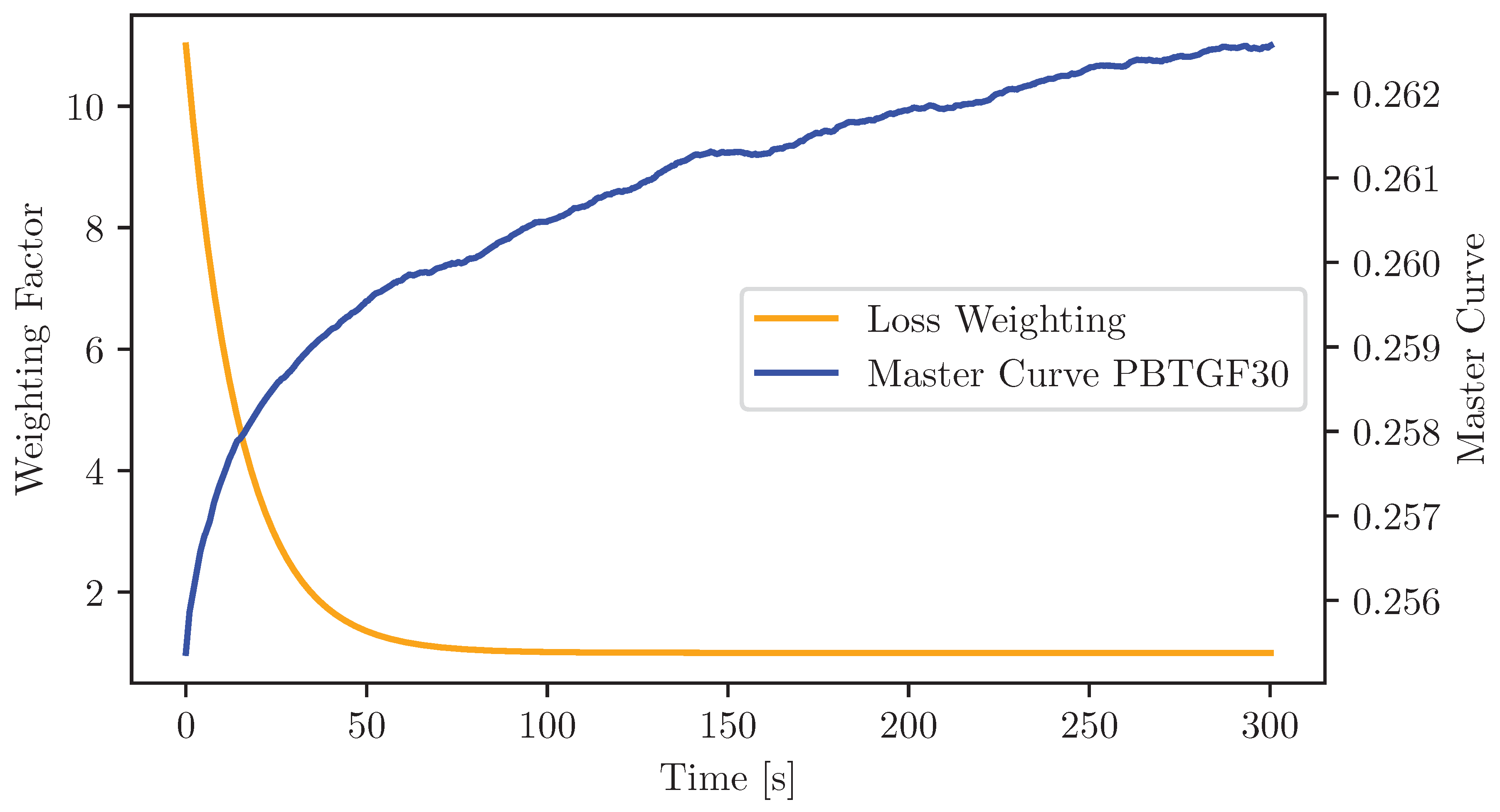
The weighting functions introduced in Section 2.2 applied during the parameter identification of the Prony series and the fractional viscoelastic models are illustrated in Figure A1 and Figure A2. Both diagrams show that the weighting factor is initially high and decreases rapidly within the first 50-70 seconds of the experimental time range. This reflects the higher sensitivity of the fitting process to the early creep stage. For reference, the experimental master curves are plotted on the secondary axis, providing visual context for the time-dependent deformation behavior.
Figure A1.
Loss weighting function together with the master curves representing the average experimental creep behavior of PBT GF0 specimens.
Figure A1.
Loss weighting function together with the master curves representing the average experimental creep behavior of PBT GF0 specimens.

Figure A2.
Loss weighting function together with the master curves representing the average experimental creep behavior of PBT GF0 specimens.
Figure A2.
Loss weighting function together with the master curves representing the average experimental creep behavior of PBT GF0 specimens.
Appendix B. Detailed Results
This section provides the detailed results of the parameter identification procedure for all the investigated specimens. The parameters for each individual sample were determined using the fitting approach described in Section 2.2. The following subsections contain tabulated values for both materials, PBT GF0 and PBT GF30, based on their respective model fits. In addition, a comparison of the mean L1 loss values for both materials is presented to assess the relative fit performance between the Prony series and the fractional viscoelastic models.
Appendix B.1. Detailed Results for PBT GF0

Table A1.
Mean L1 Loss Comparison for PBTGF0
| Smp. | Fractional Damper |
Prony 1 | %diff | Prony 2 | %diff | Prony 3 | %diff |
|---|---|---|---|---|---|---|---|
| 0 | 4.51e-04 | 6.50e-04 | 44.2% | 2.35e-04 | -47.9% | 2.14e-04 | -52.5% |
| 1 | 4.06e-04 | 6.68e-04 | 64.4% | 2.08e-04 | -48.7% | 1.82e-04 | -55.2% |
| 2 | 3.57e-04 | 6.00e-04 | 68.1% | 1.49e-04 | -58.3% | 1.43e-04 | -59.9% |
| 3 | 3.36e-04 | 7.76e-04 | 130.8% | 3.06e-04 | -9.0% | 2.53e-04 | -24.8% |
| 4 | 3.97e-04 | 8.16e-04 | 105.5% | 1.97e-04 | -50.4% | 1.97e-04 | -50.4% |
| 5 | 3.37e-04 | 6.57e-04 | 95.1% | 2.22e-04 | -34.0% | 2.02e-04 | -39.9% |
| 6 | 2.98e-04 | 8.18e-04 | 174.5% | 1.87e-04 | -37.2% | 1.87e-04 | -37.2% |
| 7 | 2.47e-04 | 6.44e-04 | 161.4% | 2.28e-04 | -7.7% | 1.91e-04 | -22.5% |
| 8 | 2.32e-04 | 5.60e-04 | 141.0% | 1.64e-04 | -29.5% | 1.57e-04 | -32.5% |
| 9 | 3.45e-04 | 7.97e-04 | 130.7% | 1.52e-04 | -56.1% | 1.52e-04 | -56.1% |
| 10 | 2.73e-04 | 5.90e-04 | 116.2% | 1.47e-04 | -46.2% | 1.47e-04 | -46.2% |
| 11 | 4.39e-04 | 5.48e-04 | 24.8% | 2.34e-04 | -46.8% | 2.06e-04 | -53.1% |
| 12 | 4.78e-04 | 6.12e-04 | 28.0% | 1.63e-04 | -65.9% | 1.63e-04 | -65.9% |
| 13 | 3.02e-04 | 6.31e-04 | 109.0% | 1.99e-04 | -34.0% | 1.73e-04 | -42.8% |
| 14 | 3.44e-04 | 5.67e-04 | 64.8% | 2.54e-04 | -26.1% | 2.41e-04 | -29.9% |
| 15 | 3.39e-04 | 7.14e-04 | 110.3% | 3.44e-04 | 1.3% | 1.79e-04 | -47.2% |
| 16 | 5.21e-04 | 6.25e-04 | 19.9% | 2.72e-04 | -47.7% | 1.79e-04 | -65.7% |
| 17 | 3.09e-04 | 9.01e-04 | 191.6% | 1.93e-04 | -37.5% | 1.81e-04 | -41.4% |
| 18 | 4.16e-04 | 5.25e-04 | 26.0% | 1.65e-04 | -60.3% | 1.65e-04 | -60.3% |
| 19 | 4.73e-04 | 5.85e-04 | 23.7% | 1.90e-04 | -59.9% | 1.80e-04 | -61.9% |
| Average | 3.65e-04 | 6.64e-04 | 91.5% | 2.10e-04 | -40.1% | 1.85e-04 | -47.3% |
Table A2.
Parameters for FractionalDamper - PBTGF0
| Sample | C | |
|---|---|---|
| 0 | 7.93e+05 | 0.44 |
| 1 | 4.19e+05 | 0.32 |
| 2 | 5.70e+05 | 0.35 |
| 3 | 4.59e+05 | 0.35 |
| 4 | 4.16e+05 | 0.32 |
| 5 | 4.60e+05 | 0.34 |
| 6 | 4.35e+05 | 0.32 |
| 7 | 4.19e+05 | 0.31 |
| 8 | 8.57e+05 | 0.41 |
| 9 | 6.31e+05 | 0.39 |
| 10 | 6.99e+05 | 0.39 |
| 11 | 5.19e+05 | 0.35 |
| 12 | 4.85e+05 | 0.35 |
| 13 | 6.11e+05 | 0.37 |
| 14 | 4.60e+05 | 0.31 |
| 15 | 2.55e+05 | 0.24 |
| 16 | 3.34e+05 | 0.29 |
| 17 | 3.55e+05 | 0.31 |
| 18 | 7.73e+05 | 0.42 |
| 19 | 7.31e+05 | 0.42 |
Table A3.
Parameters for Prony 1 - PBTGF0
| Sample | ||||
|---|---|---|---|---|
| 0 | 2644 | 97 | 46 | 2741 |
| 1 | 2625 | 84 | 27 | 2709 |
| 2 | 2638 | 75 | 32 | 2713 |
| 3 | 2534 | 88 | 38 | 2623 |
| 4 | 2614 | 83 | 25 | 2697 |
| 5 | 2622 | 87 | 35 | 2710 |
| 6 | 2610 | 82 | 29 | 2692 |
| 7 | 2653 | 77 | 38 | 2730 |
| 8 | 2602 | 77 | 51 | 2679 |
| 9 | 2604 | 87 | 35 | 2691 |
| 10 | 2544 | 74 | 45 | 2618 |
| 11 | 2600 | 83 | 37 | 2683 |
| 12 | 2583 | 87 | 34 | 2671 |
| 13 | 2642 | 83 | 42 | 2725 |
| 14 | 2625 | 70 | 27 | 2695 |
| 15 | 2637 | 79 | 21 | 2716 |
| 16 | 2579 | 86 | 25 | 2665 |
| 17 | 2593 | 90 | 28 | 2683 |
| 18 | 2587 | 83 | 44 | 2670 |
| 19 | 2619 | 93 | 43 | 2712 |
Table A4.
Parameters for Prony 2 - PBTGF0
| Sample | ||||||
|---|---|---|---|---|---|---|
| 0 | 2627 | 89 | 120 | 34 | 8 | 2749 |
| 1 | 2609 | 64 | 116 | 44 | 7 | 2716 |
| 2 | 2622 | 60 | 127 | 37 | 8 | 2719 |
| 3 | 2516 | 82 | 118 | 36 | 5 | 2634 |
| 4 | 2572 | 77 | 279 | 53 | 10 | 2703 |
| 5 | 2609 | 75 | 99 | 36 | 5 | 2720 |
| 6 | 2589 | 71 | 137 | 43 | 6 | 2703 |
| 7 | 2638 | 71 | 110 | 33 | 4 | 2742 |
| 8 | 2579 | 76 | 174 | 30 | 10 | 2685 |
| 9 | 2568 | 84 | 216 | 46 | 10 | 2698 |
| 10 | 2522 | 67 | 180 | 33 | 13 | 2622 |
| 11 | 2591 | 69 | 88 | 30 | 7 | 2690 |
| 12 | 2564 | 62 | 156 | 48 | 14 | 2675 |
| 13 | 2627 | 76 | 119 | 31 | 6 | 2734 |
| 14 | 2593 | 63 | 252 | 43 | 10 | 2700 |
| 15 | 2630 | 66 | 50 | 42 | 2 | 2738 |
| 16 | 2571 | 67 | 64 | 37 | 4 | 2675 |
| 17 | 2569 | 79 | 138 | 47 | 6 | 2695 |
| 18 | 2574 | 72 | 113 | 30 | 9 | 2675 |
| 19 | 2587 | 79 | 223 | 50 | 17 | 2716 |
Table A5.
Parameters for Prony 3 - PBTGF0
| Sample | ||||||||
|---|---|---|---|---|---|---|---|---|
| 0 | 2606 | 86 | 245 | 37 | 29 | 21 | 4 | 2750 |
| 1 | 2571 | 81 | 416 | 41 | 23 | 25 | 4 | 2718 |
| 2 | 2618 | 59 | 164 | 38 | 12 | 8 | 1 | 2722 |
| 3 | 2478 | 99 | 337 | 38 | 20 | 22 | 2 | 2637 |
| 4 | 2572 | 77 | 279 | 0 | 10 | 53 | 10 | 2703 |
| 5 | 2596 | 72 | 180 | 39 | 15 | 17 | 1 | 2725 |
| 6 | 2589 | 71 | 137 | 0 | 10 | 43 | 6 | 2703 |
| 7 | 2575 | 106 | 623 | 35 | 39 | 28 | 3 | 2743 |
| 8 | 2500 | 122 | 1000 | 36 | 85 | 27 | 9 | 2685 |
| 9 | 2568 | 84 | 216 | 0 | 24 | 46 | 10 | 2698 |
| 10 | 2522 | 67 | 180 | 0 | 67 | 33 | 13 | 2622 |
| 11 | 2571 | 65 | 242 | 46 | 20 | 15 | 1 | 2696 |
| 12 | 2564 | 62 | 156 | 7 | 14 | 42 | 14 | 2675 |
| 13 | 2612 | 75 | 215 | 30 | 22 | 18 | 3 | 2735 |
| 14 | 2507 | 141 | 1000 | 44 | 17 | 15 | 1 | 2708 |
| 15 | 2615 | 53 | 169 | 39 | 14 | 34 | 1 | 2741 |
| 16 | 2560 | 53 | 155 | 48 | 15 | 20 | 1 | 2681 |
| 17 | 2562 | 80 | 177 | 13 | 1 | 42 | 9 | 2698 |
| 18 | 2574 | 72 | 113 | 0 | 69 | 30 | 9 | 2675 |
| 19 | 2480 | 172 | 964 | 58 | 26 | 8 | 3 | 2718 |
Appendix B.2. Detailed Results for PBT GF30
Table A6.
Mean L1 Loss Comparison for PBTGF30
| Smp. | Fractional Damper |
Prony 1 | %diff | Prony 2 | %diff | Prony 3 | %diff |
|---|---|---|---|---|---|---|---|
| 0 | 3.65e-04 | 5.44e-04 | 48.8% | 1.40e-04 | -61.7% | 1.39e-04 | -61.8% |
| 1 | 2.79e-04 | 3.67e-04 | 31.4% | 1.19e-04 | -57.4% | 1.18e-04 | -57.6% |
| 2 | 2.18e-04 | 5.52e-04 | 153.9% | 1.51e-04 | -30.8% | 1.51e-04 | -30.8% |
| 3 | 2.06e-04 | 3.87e-04 | 87.8% | 1.26e-04 | -38.8% | 1.23e-04 | -40.6% |
| 4 | 2.96e-04 | 3.82e-04 | 29.3% | 1.61e-04 | -45.5% | 1.61e-04 | -45.5% |
| 5 | 2.06e-04 | 3.14e-04 | 52.1% | 2.17e-04 | 5.3% | 2.03e-04 | -1.7% |
| 6 | 3.23e-04 | 3.85e-04 | 19.2% | 1.54e-04 | -52.5% | 1.54e-04 | -52.3% |
| 7 | 2.36e-04 | 4.47e-04 | 89.1% | 1.51e-04 | -36.3% | 1.51e-04 | -36.3% |
| 8 | 3.54e-04 | 3.83e-04 | 8.1% | 2.41e-04 | -31.8% | 2.15e-04 | -39.4% |
| 9 | 2.10e-04 | 3.74e-04 | 77.7% | 1.49e-04 | -29.0% | 1.49e-04 | -29.0% |
| 10 | 2.06e-04 | 5.77e-04 | 179.6% | 1.52e-04 | -26.2% | 1.46e-04 | -29.4% |
| 11 | 3.62e-04 | 5.83e-04 | 61.2% | 1.60e-04 | -55.8% | 1.60e-04 | -55.8% |
| 12 | 2.41e-04 | 3.73e-04 | 54.6% | 1.31e-04 | -45.6% | 1.31e-04 | -45.7% |
| 13 | 2.32e-04 | 4.75e-04 | 104.3% | 1.43e-04 | -38.5% | 1.29e-04 | -44.5% |
| 14 | 3.10e-04 | 5.17e-04 | 66.5% | 1.70e-04 | -45.1% | 1.68e-04 | -45.8% |
| 15 | 2.62e-04 | 3.17e-04 | 21.3% | 2.05e-04 | -21.8% | 1.83e-04 | -30.3% |
| 16 | 2.51e-04 | 4.60e-04 | 83.6% | 1.59e-04 | -36.4% | 1.59e-04 | -36.4% |
| 17 | 2.59e-04 | 5.80e-04 | 124.1% | 2.15e-04 | -16.8% | 1.94e-04 | -25.0% |
| 18 | 2.50e-04 | 3.73e-04 | 49.6% | 2.28e-04 | -8.5% | 2.28e-04 | -8.5% |
| 19 | 2.67e-04 | 5.01e-04 | 87.5% | 1.91e-04 | -28.6% | 1.61e-04 | -39.9% |
| Average | 2.67e-04 | 4.44e-04 | 71.5% | 1.68e-04 | -35.1% | 1.61e-04 | -37.8% |
Table A7.
Parameters for FractionalDamper - PBTGF30
| Sample | C | |
|---|---|---|
| 0 | 2.33e+06 | 0.35 |
| 1 | 3.89e+06 | 0.40 |
| 2 | 2.95e+06 | 0.37 |
| 3 | 3.55e+06 | 0.39 |
| 4 | 4.84e+06 | 0.44 |
| 5 | 3.84e+06 | 0.38 |
| 6 | 4.27e+06 | 0.44 |
| 7 | 5.16e+06 | 0.47 |
| 8 | 2.94e+06 | 0.38 |
| 9 | 5.83e+06 | 0.46 |
| 10 | 2.53e+06 | 0.35 |
| 11 | 3.13e+06 | 0.42 |
| 12 | 4.38e+06 | 0.44 |
| 13 | 2.77e+06 | 0.37 |
| 14 | 2.76e+06 | 0.37 |
| 15 | 2.92e+06 | 0.36 |
| 16 | 3.25e+06 | 0.39 |
| 17 | 2.63e+06 | 0.36 |
| 18 | 4.41e+06 | 0.40 |
| 19 | 2.64e+06 | 0.35 |
Table A8.
Parameters for Prony 1 - PBTGF30
| Sample | ||||
|---|---|---|---|---|
| 0 | 9203 | 232 | 26 | 9435 |
| 1 | 9463 | 197 | 39 | 9660 |
| 2 | 9311 | 209 | 36 | 9520 |
| 3 | 9259 | 198 | 46 | 9456 |
| 4 | 9295 | 196 | 47 | 9491 |
| 5 | 9201 | 171 | 68 | 9372 |
| 6 | 9320 | 228 | 49 | 9548 |
| 7 | 9262 | 222 | 53 | 9485 |
| 8 | 9225 | 224 | 49 | 9449 |
| 9 | 9340 | 198 | 59 | 9538 |
| 10 | 9231 | 206 | 36 | 9436 |
| 11 | 9290 | 263 | 38 | 9553 |
| 12 | 9312 | 221 | 54 | 9533 |
| 13 | 9212 | 213 | 38 | 9425 |
| 14 | 9316 | 230 | 34 | 9546 |
| 15 | 9285 | 203 | 52 | 9487 |
| 16 | 9236 | 216 | 43 | 9452 |
| 17 | 9348 | 219 | 38 | 9567 |
| 18 | 9370 | 174 | 48 | 9544 |
| 19 | 9300 | 201 | 35 | 9501 |
Table A9.
Parameters for Prony 2 - PBTGF30
| Sample | ||||||
|---|---|---|---|---|---|---|
| 0 | 9123 | 177 | 214 | 148 | 11 | 9448 |
| 1 | 9373 | 184 | 276 | 112 | 16 | 9668 |
| 2 | 9231 | 201 | 199 | 106 | 9 | 9539 |
| 3 | 9226 | 183 | 113 | 67 | 6 | 9477 |
| 4 | 8965 | 408 | 1000 | 123 | 23 | 9496 |
| 5 | 9160 | 186 | 154 | 52 | 4 | 9398 |
| 6 | 9148 | 280 | 436 | 128 | 21 | 9556 |
| 7 | 9197 | 222 | 172 | 82 | 10 | 9502 |
| 8 | 9196 | 196 | 107 | 69 | 10 | 9461 |
| 9 | 9102 | 345 | 609 | 99 | 21 | 9546 |
| 10 | 9174 | 195 | 143 | 95 | 5 | 9464 |
| 11 | 9200 | 232 | 200 | 137 | 12 | 9568 |
| 12 | 9246 | 208 | 187 | 90 | 15 | 9544 |
| 13 | 9179 | 191 | 102 | 83 | 5 | 9453 |
| 14 | 9244 | 191 | 185 | 125 | 12 | 9560 |
| 15 | 9268 | 195 | 83 | 56 | 2 | 9520 |
| 16 | 9176 | 204 | 158 | 91 | 9 | 9471 |
| 17 | 9213 | 256 | 298 | 115 | 10 | 9584 |
| 18 | 9338 | 166 | 122 | 62 | 5 | 9566 |
| 19 | 9262 | 176 | 113 | 87 | 6 | 9525 |
Table A10.
Parameters for Prony 3 - PBTGF30
| Sample | ||||||||
|---|---|---|---|---|---|---|---|---|
| 0 | 9105 | 187 | 265 | 13 | 1 | 149 | 12 | 9454 |
| 1 | 9356 | 181 | 355 | 22 | 100 | 110 | 16 | 9668 |
| 2 | 9231 | 179 | 199 | 23 | 198 | 106 | 9 | 9539 |
| 3 | 9218 | 179 | 132 | 63 | 10 | 22 | 1 | 9483 |
| 4 | 8965 | 408 | 1000 | 0 | 17 | 123 | 23 | 9496 |
| 5 | 8929 | 341 | 1000 | 80 | 71 | 48 | 3 | 9398 |
| 6 | 9141 | 233 | 535 | 57 | 226 | 125 | 20 | 9556 |
| 7 | 9197 | 151 | 172 | 71 | 171 | 82 | 10 | 9502 |
| 8 | 8976 | 330 | 764 | 139 | 31 | 32 | 1 | 9477 |
| 9 | 9047 | 322 | 926 | 78 | 342 | 99 | 21 | 9546 |
| 10 | 9151 | 202 | 196 | 80 | 10 | 37 | 2 | 9470 |
| 11 | 9200 | 217 | 200 | 15 | 197 | 137 | 12 | 9568 |
| 12 | 9193 | 234 | 320 | 106 | 23 | 17 | 2 | 9550 |
| 13 | 9162 | 177 | 147 | 58 | 19 | 59 | 3 | 9456 |
| 14 | 9215 | 204 | 262 | 120 | 16 | 24 | 4 | 9563 |
| 15 | 9082 | 248 | 1000 | 138 | 54 | 52 | 2 | 9521 |
| 16 | 9176 | 160 | 160 | 44 | 152 | 91 | 9 | 9471 |
| 17 | 8888 | 560 | 1000 | 122 | 16 | 27 | 1 | 9597 |
| 18 | 9338 | 123 | 122 | 42 | 121 | 62 | 5 | 9566 |
| 19 | 9235 | 173 | 188 | 76 | 16 | 46 | 3 | 9530 |
Author Contributions
Conceptualization, Eduard Klatt, Bernd Zimmering, Oliver Niggemann and Natalie Rauter; methodology, Eduard Klatt and Bernd Zimmering; software, Bernd Zimmering and Eduard Klatt; validation, Eduard Klatt and Bernd Zimmering; formal analysis, Bernd Zimmering and Eduard Klatt; investigation, Eduard Klatt; resources, Natalie Rauter and Oliver Niggemann; data curation, Bernd Zimmering and Eduard Klatt; writing—original draft preparation, Eduard Klatt and Bernd Zimmering; writing—review and editing, Eduard Klatt, Bernd Zimmering, Oliver Niggemann and Natalie Rauter; visualization, Eduard Klatt and Bernd Zimmering; supervision, Natalie Rauter and Oliver Niggemann; project administration, Natalie Rauter and Oliver Niggemann; funding acquisition, Natalie Rauter and Oliver Niggemann; All authors have read and agreed to the published version of the manuscript.
Funding
This publication has been funded by the Open-Access-Publication-Fund of the Helmut-Schmidt-University/University of the Federal Armed Forces Hamburg.
Data Availability Statement
All code and data necessary to reproduce the results of this study are available at the following anonymous repository: https://anonymous.4open.science/r/PBTGF_Creep-4D5A. This link has been anonymized for peer review and will be replaced by a non-anonymous link to a GitHub repository upon acceptance. License under which the data set is made available (CC BY-NC-SA 4.0)
Acknowledgments
During the preparation of this manuscript, the authors used ChatGPT-4o for the purpose of improving English language, grammar, and style. The authors take full responsibility for the content of this publication.
Conflicts of Interest
The authors declare no conflicts of interest.
Abbreviations
The following abbreviations are used in this manuscript:
| AD | Automatic Differentiation |
| L-BFGS-B | Limited Memory Broyden–Fletcher–Goldfarb–Shanno Method |
| DIC | Digital image correlation |
| FEM | Finite Element Method |
| IVP | Initial value Problem |
| NFDE | Neural Fractional Differential Equation |
| ODE | Ordinary Differential Equation |
| PBT | Polybutylene terephthalate (thermoplastic material) |
| PBT GF0 | Polybutylene terephthalate without fibre content |
| PBT GF30 | Polybutylene terephthalate with 30% fibre mass fraction |
| SFRC | Short fibre-reinforced composite |
References
- Osswald, T.A.; Menges, G. Materials science of polymers for engineers; Carl Hanser Verlag GmbH Co KG, 2012. [CrossRef]
- Mark, J. Physical Properties of Polymers Handbook; Springer New York, 2007.
- Tomar, N.; Maiti, S.N. Mechanical properties of PBT/ABAS blends. Journal of Applied Polymer Science 2007, 104, 1807–1817. [Google Scholar] [CrossRef]
- Domininghaus, H. Kunststoffe: Eigenschaften und Anwendungen; Springer Berlin Heidelberg, 2012. [CrossRef]
- Schürmann, H. Konstruieren mit Faser-Kunststoff-Verbunden; Springer, 2007. [CrossRef]
- Li, Q. Three Dimensional Numerical Simulation of Melt Filling Process in Mold Cavity with Insets. Procedia Engineering 2015, 126, 496–501. [Google Scholar] [CrossRef]
- von Bradsky, G.J.; Bailey, R.S.; Cervenka, A.J.; Zachmann, H.G.; Allan, P.S. Characterization of finite length composites: Part IV - Structural studies on injection moulded composites (Technical Report). Pure and Applied Chemistry 1997, 69, 2523–2540. [Google Scholar] [CrossRef]
- Huang, C.T.; Chen, X.W.; Fu, W.W. Investigation on the Fiber Orientation Distributions and Their Influence on the Mechanical Property of the Co-Injection Molding Products. Polymers 2020, 12. [Google Scholar] [CrossRef]
- Kaliske, M. A formulation of elasticity and viscoelasticity for fibre reinforced material at small and finite strains. Computer Methods in Applied Mechanics and Engineering 2000, 185, 225–243. [Google Scholar] [CrossRef]
- Chen, Y.; Zhao, Z.; Li, D.; Guo, Z.; Dong, L. Constitutive modeling for linear viscoelastic fiber-reinforced composites. Composite Structures 2021, 263, 113679. [Google Scholar] [CrossRef]
- Cruz-González, O.; Ramírez-Torres, A.; Rodríguez-Ramos, R.; Otero, J.; Penta, R.; Lebon, F. Effective behavior of long and short fiber-reinforced viscoelastic composites. Applications in Engineering Science 2021, 6, 100037. [Google Scholar] [CrossRef]
- Tschoegl, N.W. The phenomenological theory of linear viscoelastic behavior: an introduction; Springer Berlin, Heidelberg, 1989. [CrossRef]
- Wineman, A.; Rajagopal, K. Mechanical Response of Polymers: An Introduction; Mechanical Response of Polymers: An Introduction, Cambridge University Press, 2000.
- COMSOL. Structural Mechanics Module User’s Guide. Stockholm, Sweden, 2023.
- Dassault Systèmes. Abaqus 6.14 Analysis User’s Guide. Providence, RI, USA, 2014.
- Effinger, V.M. Finite nichtlinear viskoelastische Modellierung offenzelliger Polymerschäume. PhD thesis, Stuttgart: Institut für Baustatik und Baudynamik, Universität Stuttgart, 2016.
- Gutierrez-Lemini, D. Engineering Viscoelasticity; SpringerLink : Bücher, Springer US, 2013.
- Endo, V.T.; de Carvalho Pereira, J.C. Linear orthotropic viscoelasticity model for fiber reinforced thermoplastic material based on Prony series. Mechanics of Time-Dependent Materials 2017, 21, 199–221. [Google Scholar] [CrossRef]
- Bhangale, N.; Kachhia, K.B.; Gómez-Aguilar, J.F. Fractional viscoelastic models with Caputo generalized fractional derivative. Mathematical Methods in the Applied Sciences 2023, 46, 7835–7846. [Google Scholar] [CrossRef]
- Chen, W.; Sun, H.; Li, X.; et al. Fractional derivative modeling in mechanics and engineering; Springer, 2022.
- Xu, Y.; Dong, Y.; Huang, X.; Luo, Y.; Zhao, S. Properties Tests and Mathematical Modeling of Viscoelastic Damper at Low Temperature With Fractional Order Derivative. Frontiers in Materials 2019, 6. [Google Scholar] [CrossRef]
- Kontou, E.; Katsourinis, S. Application of a fractional model for simulation of the viscoelastic functions of polymers. J. Appl. Polym. Sci. 2016, 133, https. [Google Scholar] [CrossRef]
- Coelho, C.; P. Costa, M.F.; Ferrás, L. Neural fractional differential equations. Applied Mathematical Modelling 2025, 144, 116060. [CrossRef]
- Zimmering, B.; Coelho, C.; Niggemann, O. Optimising Neural Fractional Differential Equations for Performance and Efficiency. In Proceedings of the Proceedings of the 1st ECAI Workshop on "Machine Learning Meets Differential Equations: From Theory to Applications"; Coelho, C.; Zimmering, B.; Costa, M.F.P.; Ferrás, L.L.; Niggemann, O., Eds. PMLR, 20 Oct 2024, Vol. 255, Proceedings of Machine Learning Research, pp. 1–22.
- Lakes, R.S. Viscoelastic solids; Vol. 9, CRC press, 1998.
- Phan-Thien, N. Understanding Viscoelasticity - Basics of Rheology; Springer Science & Business Media: Berlin Heidelberg, 2013.
- Haddad, Y.M. Viscoelasticity of engineering materials; Springer, 1995.
- Drozdov, A.D. Finite Elasticity and Viscoelasticity; WORLD SCIENTIFIC, 1996;[https://www.worldscientific.com/doi/pdf/10.1142/2905]. [CrossRef]
- Boltzmann, L. Sitzungsber. Kgl. Akad. Wiss. Wien, Math. Naturw. Classe A 1874, 2, 70–275. [Google Scholar]
- Ferry, J.D. Viscoelastic properties of polymers; John Wiley & Sons, 1980.
- Christensen, R. Theory of Viscoelasticity: Second Edition; Dover Civil and Mechanical Engineering, Dover Publications, 2013.
- Kreider, D.; Kuller, R.; Ostberg, D. Elementary Differential Equations; Addison-Wesley series in mathematics, Addison-Wesley Publishing Company, 1968.
- Findley, W.N.; Lai, J.S.; Onaran, K. Creep and relaxation of nonlinear viscoelastic materials, with an introduction to linear viscoelasticity, 1976.
- Diethelm, K.; Ford, N.J.; Freed, A.D. A Predictor-Corrector Approach for the Numerical Solution of Fractional Differential Equations. Nonlinear Dynamics 2002, 29, 3–22. [Google Scholar] [CrossRef]
- Nocedal, J.; Wright, S.J. Numerical Optimization; Springer Series in Operations Research and Financial Engineering, Springer New York, 2006. [CrossRef]
- Paszke, A.; Gross, S.; Massa, F.; Lerer, A.; Bradbury, J.; Chanan, G.; Killeen, T.; Lin, Z.; Gimelshein, N.; Antiga, L.; et al. PyTorch: An Imperative Style, High-Performance Deep Learning Library. In Advances in Neural Information Processing Systems; Curran Associates Inc.: Red Hook, NY, USA, 2019.
- Rumelhart, D.E.; Hinton, G.E.; Williams, R.J. Learning Representations by Back-Propagating Errors. Nature 1986, 323, 533–536. [Google Scholar] [CrossRef]
- Baydin, Atilim Gunes and Pearlmutter, Barak A and Radul, Alexey Andreyevich and Siskind, Jeffrey Mark. Automatic Differentiation in Machine Learning: A Survey. Journal of machine learning research 2018, 18.
- Nocedal, J. Updating Quasi-Newton Matrices with Limited Storage. Mathematics of Computation 1980, 35, 773–782. [Google Scholar] [CrossRef]
- Kingma, D.P.; Ba, J. Adam: A Method for Stochastic Optimization. CoRR 2014, abs/1412.6980.
- Chung, D.D.L. Composite Materials, 2 ed.; Engineering Materials and Processes, Springer, 2010.
- Vaidya, U.K.; Chawla, K.K. Processing of fibre reinforced thermoplastic composites. International Materials Reviews 2008, 53, 185–218. [Google Scholar] [CrossRef]
- Szalai, S.; Dogossy, G. Speckle pattern optimization for DIC technologies. Acta Technica Jaurinensis 2021, 14, 228–243. [Google Scholar] [CrossRef]
- Reu, P. Introduction to Digital Image Correlation: Best Practices and Applications. Experimental Techniques 2012, 36, 3–4. [Google Scholar] [CrossRef]
- Schreier, H.; Orteu, J.J.; Sutton, M.A. Image Correlation for Shape, Motion and Deformation Measurements: Basic Concepts, Theory and Applications; Springer US, 2009. [CrossRef]
- Obaid, N.; Kortschot, M.T.; Sain, M. Understanding the Stress Relaxation Behavior of Polymers Reinforced with Short Elastic Fibers. Materials 2017, 10. [Google Scholar] [CrossRef] [PubMed]
- Drozdov, A.; Al-Mulla, A.; Gupta, R. The viscoelastic and viscoplastic behavior of polymer composites: polycarbonate reinforced with short glass fibers. Computational Materials Science 2003, 28, 16–30. [Google Scholar] [CrossRef]
- Kutty, S.K.N.; Nando, G.B. Short kevlar fiber–thermoplastic polyurethane composite. Journal of Applied Polymer Science 1991, 43, 1913–1923. [Google Scholar] [CrossRef]
- Fliegener, S.; Hohe, J. An anisotropic creep model for continuously and discontinuously fiber reinforced thermoplastics. Composites Science and Technology 2020, 194, 108168. [Google Scholar] [CrossRef]
- Burgarella, B.; Maurel-Pantel, A.; Lahellec, N.; Bouvard, J.L.; Billon, N.; Moulinec, H.; Lebon, F. Effective viscoelastic behavior of short fibers composites using virtual DMA experiments. Mechanics of Time-Dependent Materials 2019, 23, 337–360. [Google Scholar] [CrossRef]
Figure 1.
Schematic representation of the typical behaviour of creep strain divided into three distinct stages, while constant load and temperature T are applied to a specimen.
Figure 1.
Schematic representation of the typical behaviour of creep strain divided into three distinct stages, while constant load and temperature T are applied to a specimen.
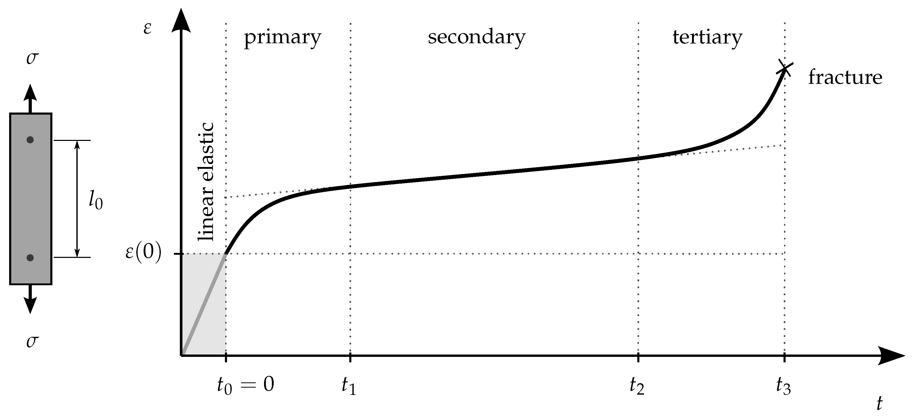
Figure 2.
Elementary rheological models of viscoelasticity.
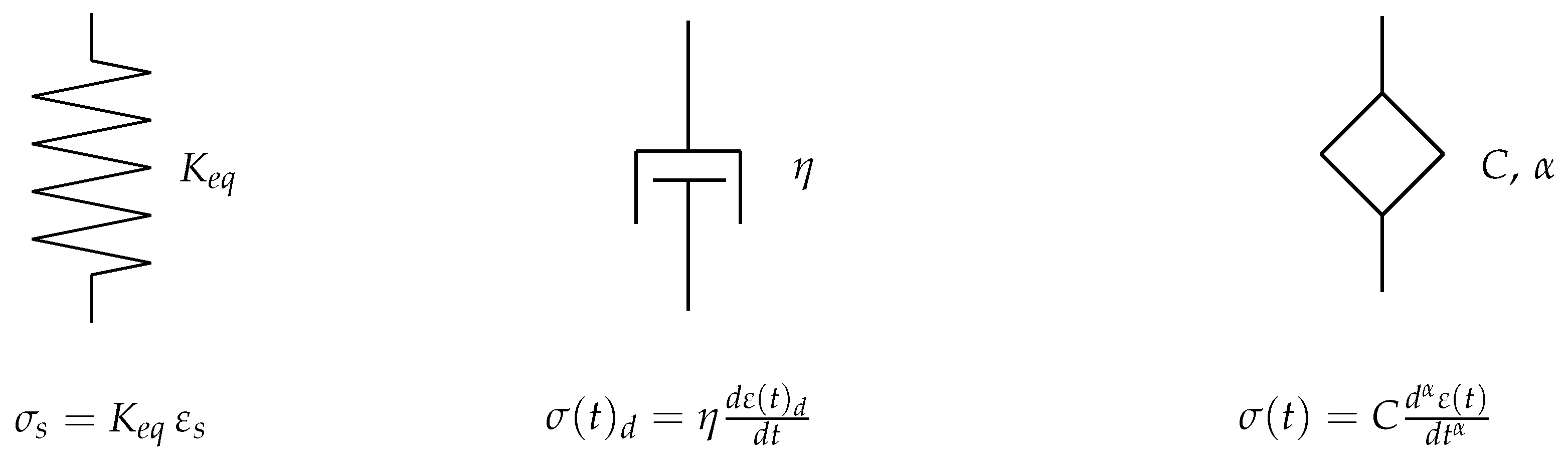
Figure 3.
Schematic representation of rheological models for viscoelasticity: (a) basic Maxwell model and (b) generalized Maxwell model.
Figure 3.
Schematic representation of rheological models for viscoelasticity: (a) basic Maxwell model and (b) generalized Maxwell model.
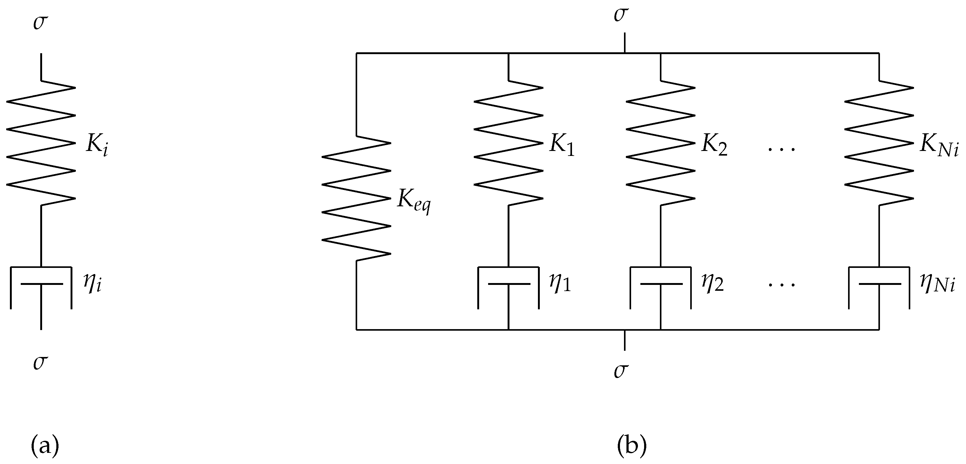
Figure 4.
Schematic representation of tensile test specimen according to DIN EN ISO 527-2 Type 1A, with maximum dimensions of .
Figure 4.
Schematic representation of tensile test specimen according to DIN EN ISO 527-2 Type 1A, with maximum dimensions of .
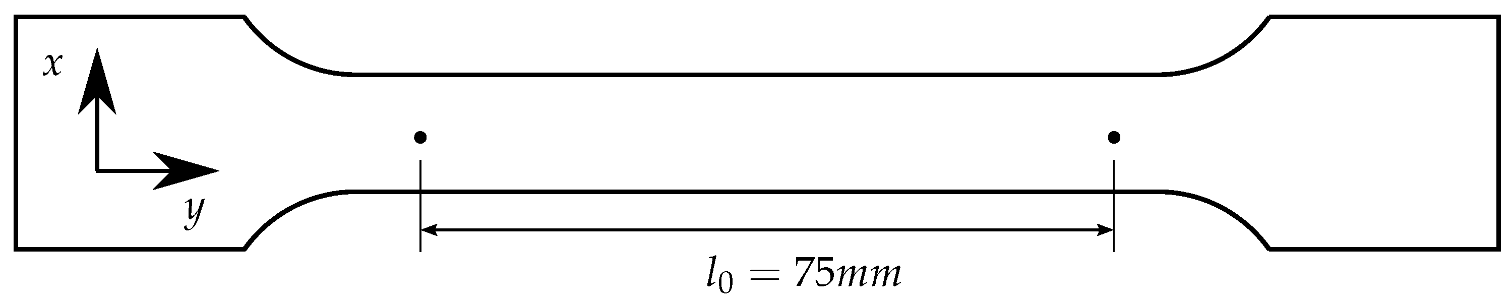
Figure 5.
Experimental setup with the ARAMIS digital image correlation system.
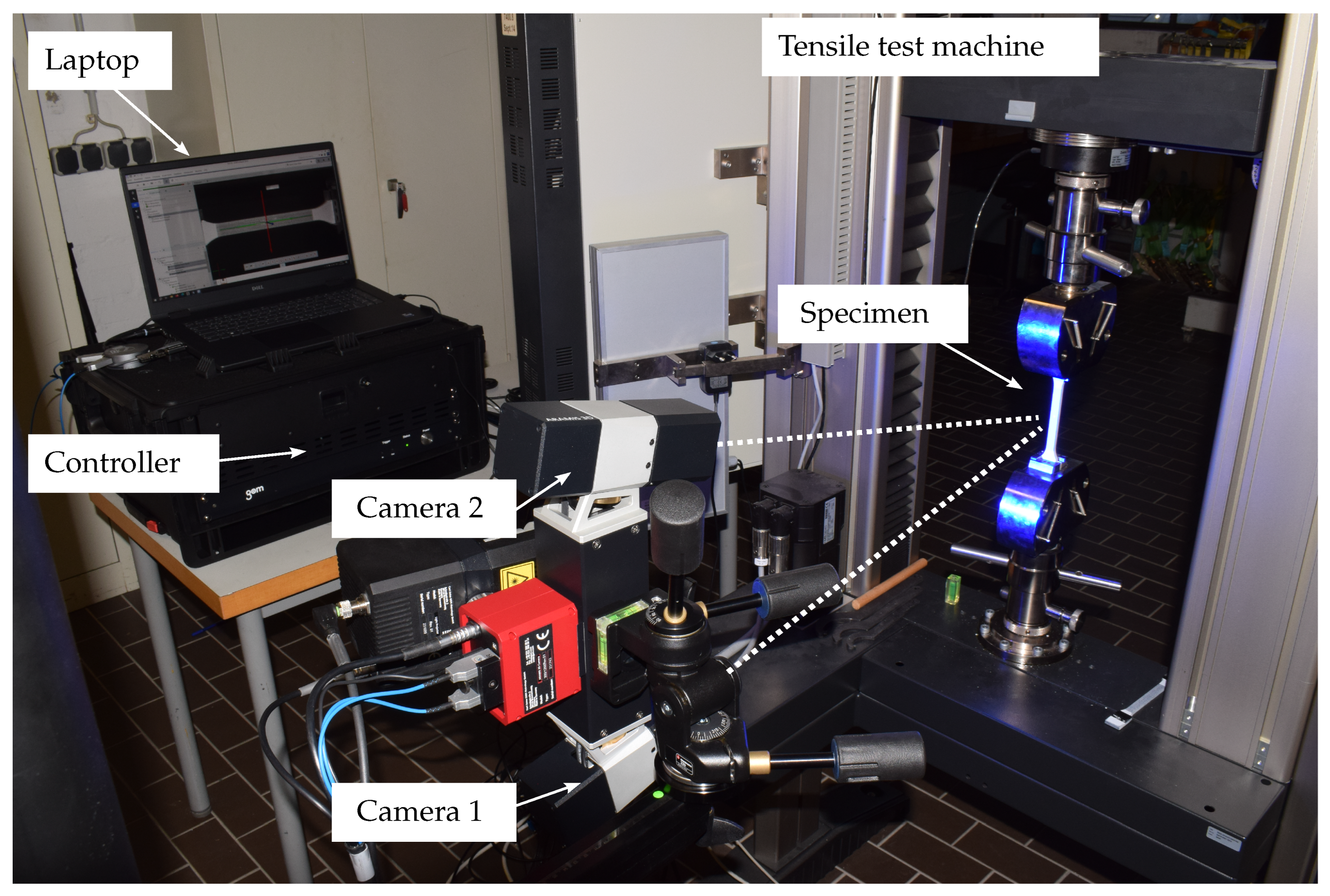
Figure 6.
Visualisation of the strain distribution of the PBT GF0 specimen under a sustained load of . (a) Speckle stochastic pattern on the specimens surface, (b) the tensile test specimen mounted in the tensile testing machine, and (c) the strain distribution () over the pre-marked surface in the x-y plane.
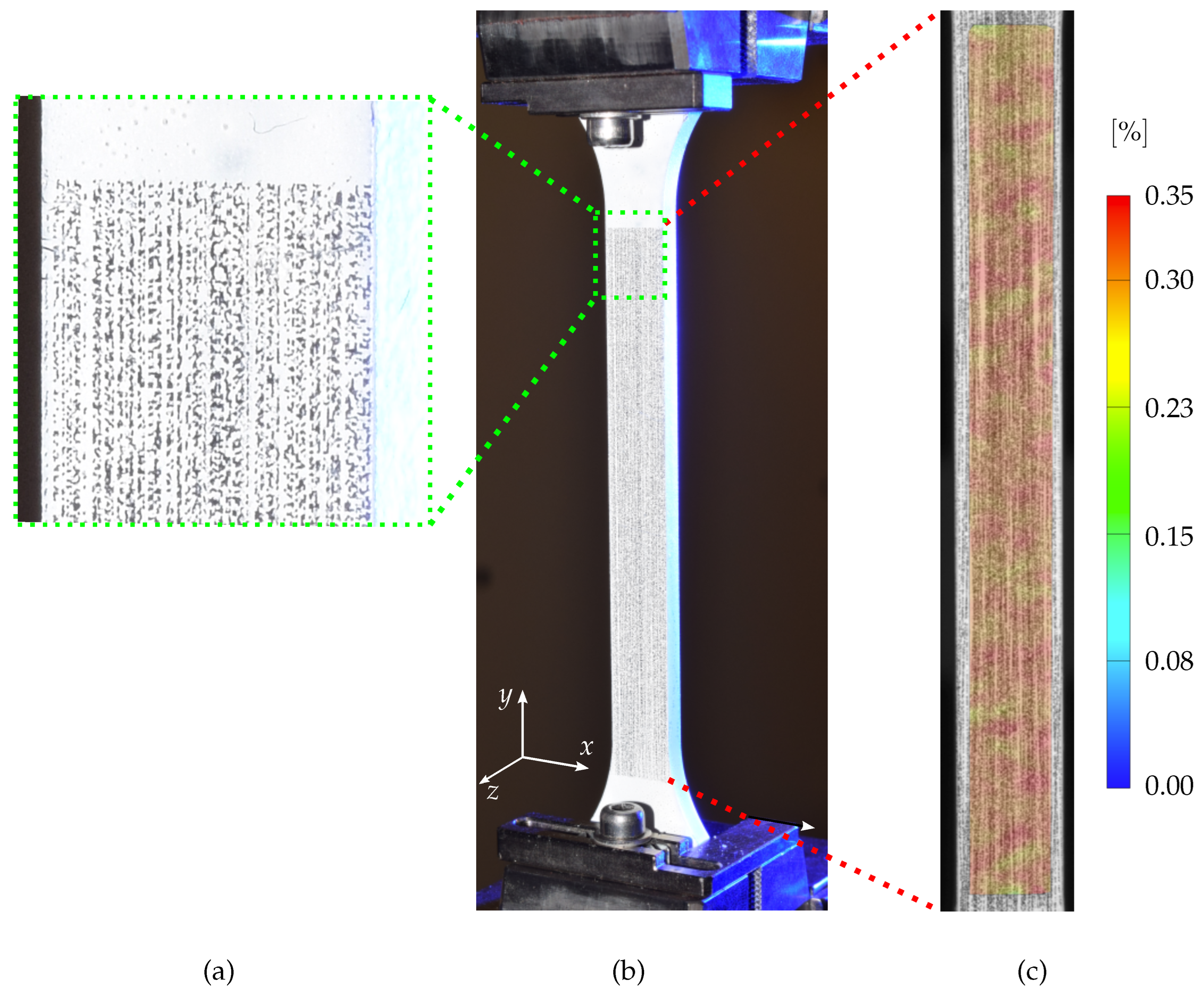
Figure 7.
Experimental creep behavior of the total strain results for 20 specimens of PBT GF0 and PBT GF30 over the test duration.
Figure 7.
Experimental creep behavior of the total strain results for 20 specimens of PBT GF0 and PBT GF30 over the test duration.
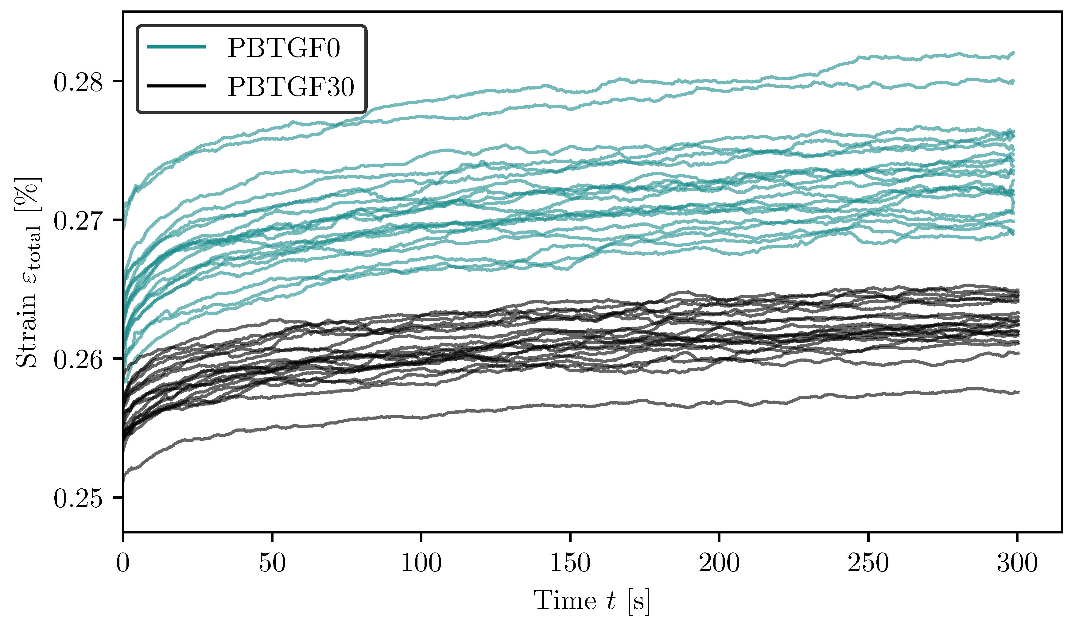
Figure 8.
Master curves representing the average experimental creep behaviour of the PBT GF0 and PBT GF30 samples.
Figure 8.
Master curves representing the average experimental creep behaviour of the PBT GF0 and PBT GF30 samples.
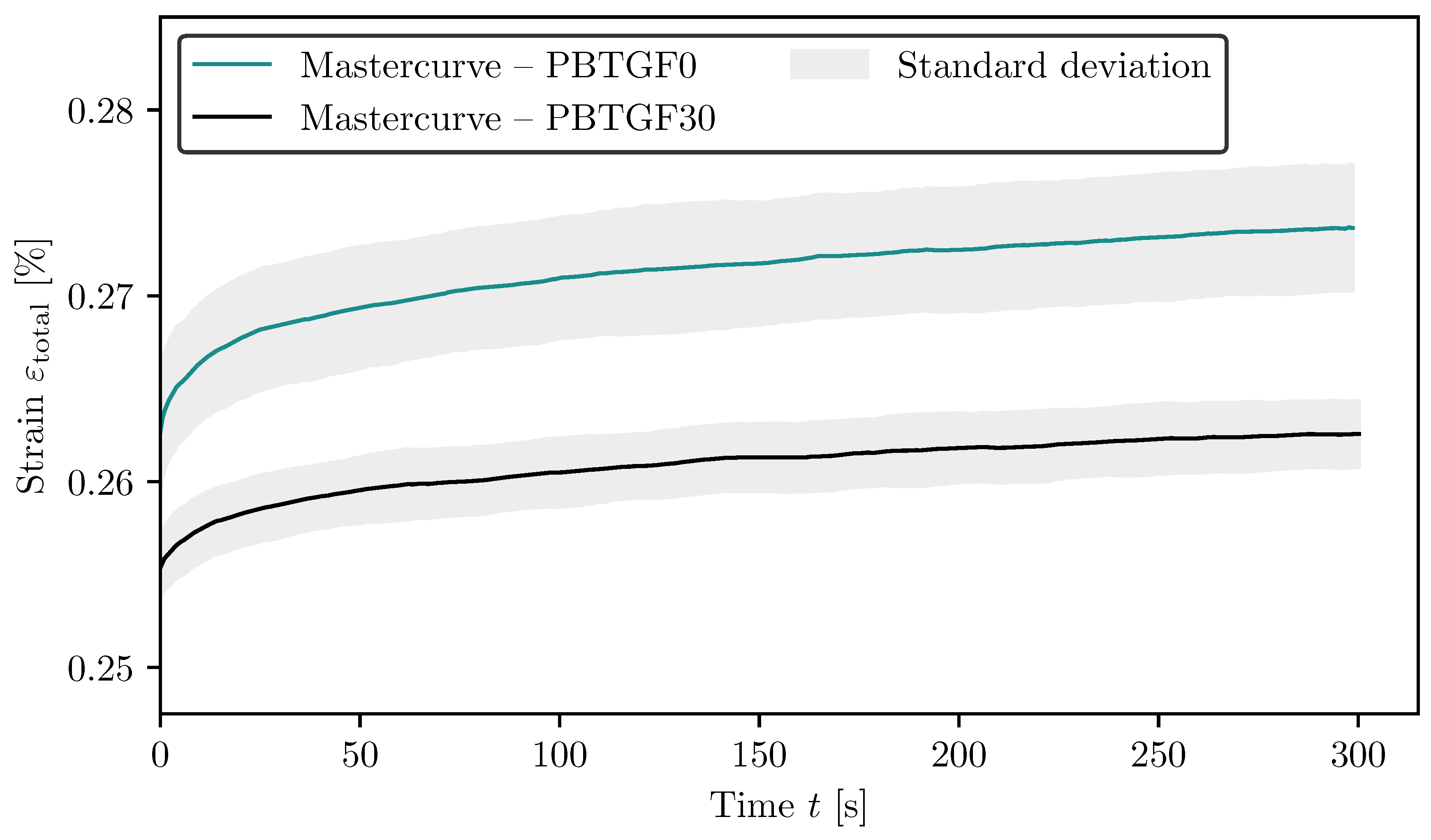
Figure 9.
Master curves representing the average experimental creep behavior according to Equation (1) of the PBT GF0 and PBT GF30 samples.
Figure 9.
Master curves representing the average experimental creep behavior according to Equation (1) of the PBT GF0 and PBT GF30 samples.
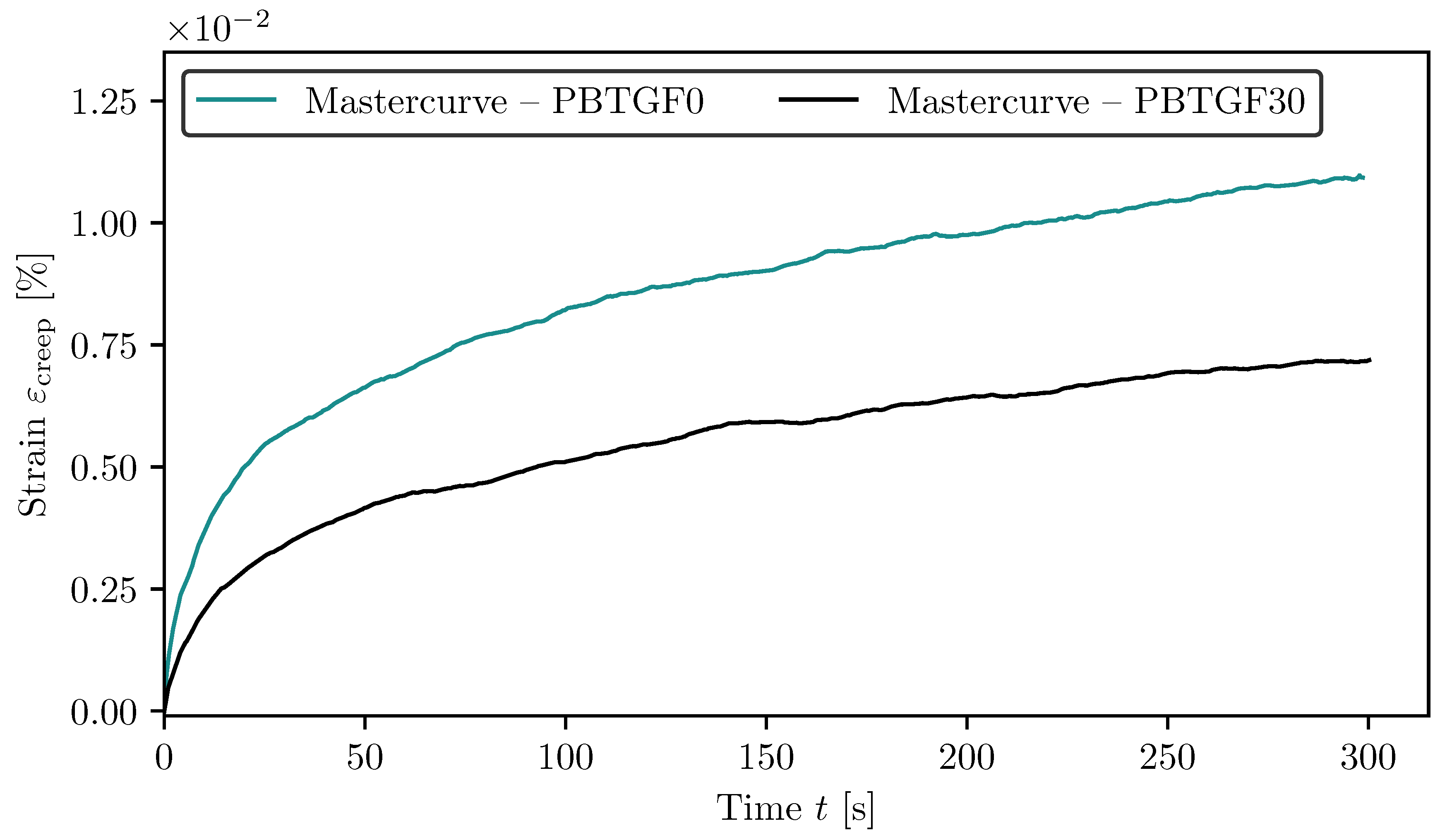
Figure 10.
Master curves representing the average experimental creep behaviour of PBT GF0 specimens. The prediction models include the Prony series model ()) with mean values from Table 2, Table 3, and Table 4 and the fractional model with mean values from Table 5.
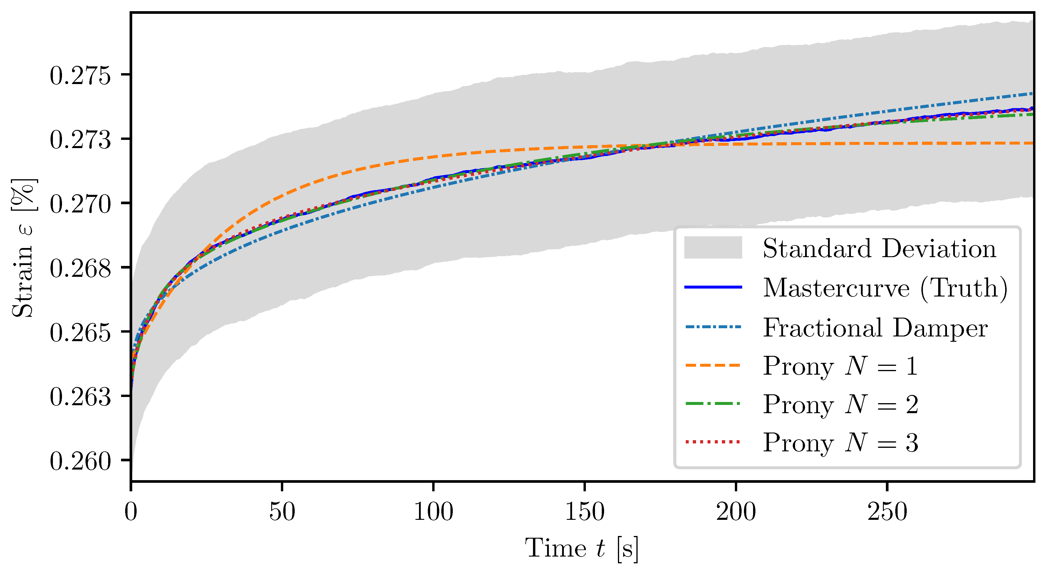
Figure 11.
Master curves representing the average experimental creep behaviour of PBT GF30 specimens. The prediction models include the Prony series model () with mean values from Table 2, Table 3, and Table 4 and the fractional model with mean values from Table 5.
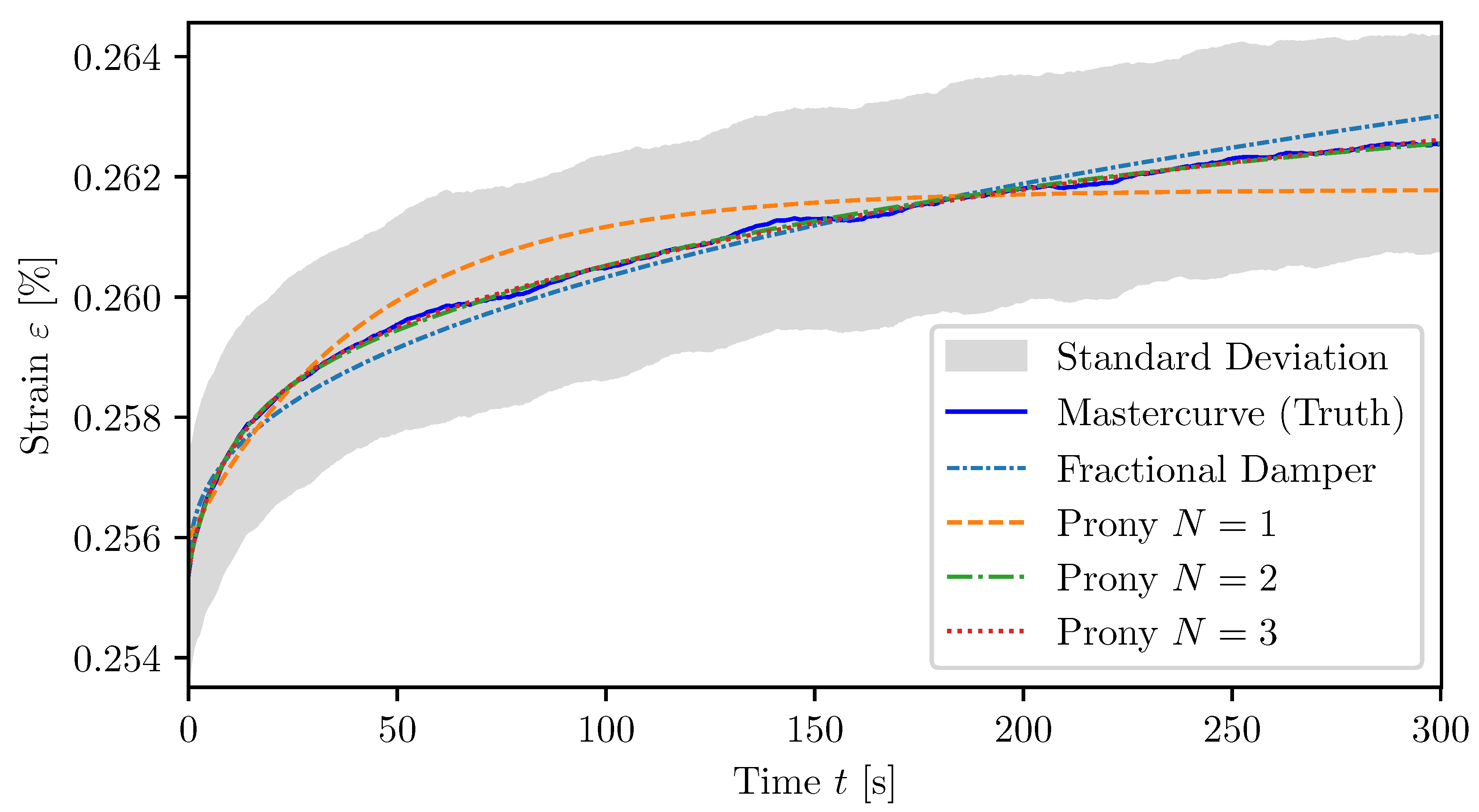
Table 1.
Summary of experimental conditions for creep behaviour testing of PBT GF0 and PBT GF30 specimens.
Table 1.
Summary of experimental conditions for creep behaviour testing of PBT GF0 and PBT GF30 specimens.
| Type of Material | Force [] | Time to Apply the Force [] | Duration of Creep Measurement [] |
|---|---|---|---|
| PBT GF0 | 300 | 3 | 300 |
| PBT GF30 | 1025 | 3 | 300 |
Table 2.
Mean values and standard deviations (Mean ± StdDev) of Prony-series coefficients for Prony 1 with 1 terms.
Table 2.
Mean values and standard deviations (Mean ± StdDev) of Prony-series coefficients for Prony 1 with 1 terms.
| Parameter | PBTGF0 | PBTGF30 |
|---|---|---|
Table 3.
Mean values and standard deviations (Mean ± StdDev) of Prony-series coefficients for Prony 2 with 2 terms.
Table 3.
Mean values and standard deviations (Mean ± StdDev) of Prony-series coefficients for Prony 2 with 2 terms.
| Parameter | PBTGF0 | PBTGF30 |
|---|---|---|
Table 4.
Mean values and standard deviations (Mean ± StdDev) of Prony-series coefficients for Prony 3 with 3 terms.
Table 4.
Mean values and standard deviations (Mean ± StdDev) of Prony-series coefficients for Prony 3 with 3 terms.
| Parameter | PBTGF0 | PBTGF30 |
|---|---|---|
Table 5.
Mean values and standard deviations (Mean ± StdDev) of Fractional Element parameters.
| Parameter | PBTGF0 | PBTGF30 |
|---|---|---|
| C | ||
Disclaimer/Publisher’s Note: The statements, opinions and data contained in all publications are solely those of the individual author(s) and contributor(s) and not of MDPI and/or the editor(s). MDPI and/or the editor(s) disclaim responsibility for any injury to people or property resulting from any ideas, methods, instructions or products referred to in the content. |
© 2025 by the authors. Licensee MDPI, Basel, Switzerland. This article is an open access article distributed under the terms and conditions of the Creative Commons Attribution (CC BY) license (http://creativecommons.org/licenses/by/4.0/).
Copyright: This open access article is published under a Creative Commons CC BY 4.0 license, which permit the free download, distribution, and reuse, provided that the author and preprint are cited in any reuse.


