
Submitted:
09 June 2025
Posted:
10 June 2025
You are already at the latest version
Abstract
The current distribution of grassland vegetation in the Colombian Orinoquia is presented and discussed through the application of machine learning techniques to multidimen-sional imagery and an empirical-statistical modeling framework. This model was devel-oped by integrating 281 vegetation surveys grouped into 18 phytosociological alliances, environmental complexes, a geomorphological gradient, bioclimatic factors, and a multi-sensor image composed of Landsat-8 bands from the visible and infrared portions of the electromagnetic spectrum, along with dual-polarization Sentinel-1 bands. Approximately 73.74% of the region still retains some form of natural vegetation, with 32.19% corre-sponding to forests and 41.55% to natural grasslands. The most prevalent alliances are Paspalo pectinati–Axonopodion aurei and Axonopodo aurei–Trachypogonion spicati, covering 6.02% and 4.37% of the area, respectively. Additionally, the ecogeographical distribution of the syntaxa and the dominance of C4 Poaceae species are discussed. Notably, Rhynchosporo barbatae–Andropogonion virgati and Sipaneo pratensis–Axonopodion purpusi stand out due to the marked dominance of C4 Poaceae among their characteristic species (50% and 60%, respectively). These findings underscore the relevance of integrating environmental complexes with bioclimatic, floristic, and physiological attributes to enhance the spatial interpretation of ecogeographical vegetation patterns at a regional scale.
Keywords:
remote sensing and vegetation mapping
; ecology of neotropical grasslands
; bioclimate and environmental gradients
; vegetation of the Colombian Orinoquia
1. Introduction
Landscape-scale studies have shown that the distribution of plant communities is correlated with soil nutrients influenced by climate and geomorphology [1,2]. Bioclimatic indices, derived from quantitative temperature and precipitation data, are valuable tools for identifying thresholds associated with climatic events that induce hydric and thermal stress, thereby affecting vegetation patterns [3, 4]. Likewise, geomorphological factors are key determinants in vegetation modeling [5, 6, 7, 8]. Together with mesoclimatic patterns, these factors constitute the main predictors of the geographical distribution of vegetation along environmental gradients [9, 10, 11, 12, 13]. Mechanistic models that integrate spectral data with climatic variables such as temperature, solar radiation, and humidity have proven effective in the spatial characterization of vegetation [14]. This approach enables a better understanding of the ecogeographical ranges of plant communities, their responses to underlying environmental conditions, historical land-use changes, and intrinsic attributes such as floristic composition, characteristic species dominance, and autoecological traits, among others.
Grasslands occupy approximately 40% of the Earth's surface, making them one of the most extensive vegetation formations globally [15]. Their environmental characteristics and biotic composition provide key ecological, economic, and cultural services [16]. However, in recent decades, significant degradation processes linked to human activities have been documented, resulting in drastic alterations in species richness, floristic composition, and the structure of original plant communities [17].
The types of vegetation present respond to variables operating at three levels: (i) environmental factors or magnitude ranges—such as climate and topography—where phytocoenoses may establish; (ii) the assemblage of plant populations present, depending on their physiological responses; and (iii) the structural and functional characteristics of vegetation types [8]. Environmental complexes also influence the ecogeographic distribution of biodiversity in three main ways: (i) by acting as limiting or regulatory factors on the ecophysiology of organisms; (ii) through disturbances that modify environmental conditions; and (iii) as sources of assimilable resources or components [18, 19].
In this context, environmental and bioclimatic gradients are considered direct drivers, as they influence species physiology and, consequently, community metabolism. C3 and C4 grasses, for instance, exhibit significant differences in their distributional patterns along ecological, climatic, edaphic, and hydric gradients, due to substantial divergences in their physiology, biochemistry, anatomy, ultrastructure, and environmental requirements [20, 21, 22]. Topographic gradients, although considered indirect factors, are nonetheless strongly correlated with vegetation distribution, despite having a lesser direct influence on some biota [23, 24, 25, 26]. As a result, accurately representing the geographical distribution of phytocoenoses remains a persistent challenge, owing to their high spatial heterogeneity at multiple scales and their differential responses to climatic, geomorphological, and anthropogenic factors [27, 28].
This article presents a characterization of the current geographical distribution of grassland vegetation in the Colombian Orinoquia, based on the integration of data from: (i) georeferenced phytosociological alliances obtained from field surveys; (ii) the environmental complex, defined by the geomorphological gradient and limiting bioclimatic factors; and (iii) multisensor imagery, composed of Landsat-8 bands from the visible and infrared portions of the electromagnetic spectrum, along with dual-polarization Sentinel-1 bands. The aim is to improve the interpretation of these vegetation types in support of the development and implementation of conservation and sustainable management strategies.
2. Materials and Methods
2.1. Study Area
The Colombian-Venezuelan Llanos represent the second-largest expanse of Neotropical savannas, covering approximately 532,000 km2 (254,000 km2 in Colombia and 278,000 km2 in Venezuela) [29, 30]. This region is notable for its floristic diversity and ecological complexity. In Colombia, it spans the departments of Arauca, Casanare, Meta, and Vichada, extending from the foothills of the Eastern Cordillera to the Orinoco River, and bounded by the Guaviare and Arauca rivers.
Its geographical boundaries are defined as follows: to the north, the Arauca River and the Venezuelan border; to the east, the Orinoco River; to the south, the Guaviare and Guayabero rivers; and to the west, the Guayabero River basin and the altitudinal limit of the Foothills (Piedemonte), which rises southward due to crustal flexure in the High Plain (Altillanura) [31].
From a geomorphological perspective, two main units are distinguished based on drainage and relief: the well-drained Orinoquia (east of the Meta River, in the departments of Meta and Vichada), characterized by dissected high plains, hills, and terraces; and the poorly drained Orinoquia (west of the Meta River, in Casanare and Arauca), marked by alluvial/eolic plains and alluvial fans [32]. Four physiographic units are recognized: the Foothills, Alluvial/Eolic Plains, High Plain, and La Macarena mountain range [32, 33, 34, 35].
2.2. Physiographic Setting.
The hydrographic zoning of Colombia [36] and the NASA SRTM v.3 digital elevation model (30 m resolution) were used within Google Earth Engine (GEE) to determine elevation ranges [37]. The Foothills zone [32] was delineated based on elevation thresholds by watershed: south of the Meta River (Guamal watershed), 575–350 m; north of the Meta, in the Meta and Pauto watersheds (675–200 m), Casanare (600–200 m), Cravo Sur (425–200 m), and Arauca (375–175 m). Its northern boundary was defined by the Arauca River and its southern boundary by the Ariari River watershed.
La Macarena was delimited by elevation thresholds of 575 m (Guayabero River) and 775 m (Guaviare River), and by the watersheds of the Ariari and Guayabero rivers. The Floodplain was identified to the west of the Foothills, bounded by the Arauca and Meta rivers and the eastern national border. The High Plain were defined as lying between the Foothills and La Macarena (to the west), the Meta River (north), the Orinoco River (east), and the Guaviare River (south) (Figure 1).
2.3. Grassland Phytosociological Framework [38].
The phytosociological classification comprises one class, three orders, and 18 alliances. The class Schizachyrio sanguinei–Trachypogonetea spicati is represented across all physiographic units of the region. It includes three orders: Axonopodo purpusi–Paspaletalia pectinati (comprising seven alliances), Schizachyrio brevifolii–Trachypogonetalia spicati (five alliances), and Axonopodo purpusi–Andropogonetalia virgati (six alliances). Their floristic composition, species richness, and ecological complexity span a wide range of environments—from piedmont foothills and dissected uplands in the high plains to aeolian flats and fluviolacustrine deposits within the alluvial plain.
2.4. Modelling Aproach. Data Sources. Mapping Framework
The adopted methodology follows an empirical–statistical modeling framework, based on the relationship between a multidimensional stack of predictor variables and grassland types as the response variable. The dataset consisted of 281 grassland relevés from the Colombian Orinoquia, compiled by Minorta-Cely et al., [38] and Rangel-Ch. et al., [39]. To model current distribution patterns, both unsupervised classification (K-means) and supervised classification (Random Forest) algorithms were applied. The former was used to define training areas, while the latter was used to predict spatial distribution. The modeling was supported by field data and integrated geomorphological variables, bioclimatic factors influencing vegetation distribution, and satellite imagery from Landsat-8 (optical) and Sentinel-1 (C-band SAR) sensors.
Bioclimatic variables were sourced from the WorldClim repository, which provides global interpolated temperature and precipitation data at 1 km resolution, derived from over 60,000 meteorological stations for the period 1970–2000 [40].
Figure 2 presents the methodological synopsis used to model the current distribution of vegetation. The input variables considered were: i) Geomorphology, which influences vegetation through factors such as solar exposure and the availability of water and nutrients; ii) Adjusted potential evapotranspiration, used as an indicator of thermal and hydric balance; iii) Annual ombrothermic index, which estimates water availability;
iv) Ombrothermic index for the driest quarter, which relates precipitation and temperature during that period; v) Thermicity index, which accounts for the influence of extreme temperatures; vi) C-band SAR data, which reflect physiognomic characteristics such as vegetation height and density; and vii) Optical sensor data, which capture the differential spectral response of grasslands in the visible and infrared ranges. The following section describes the cartographic layers used in the spatial modeling.
2.4. Data sources. Grassland Mapping
Geomorphology. Cartographic layer depicting the spatial distribution of regional-scale geomorphological units, derived from a model integrating key terrain descriptors: (i) HH/HV polarizations from an annual ALOS-PALSAR mosaic; (ii) NASA SRTM v.3 Digital Elevation Model (DEM); (iii) slope; (iv) aspect; (v) convexity; and (vi) roughness [32].
Adjusted Potential Evapotranspiration. Cartographic layer representing the maximum amount of water that can be evaporated from a vegetated soil under ideal conditions, adjusted by monthly insolation. Its calculation involved: (i) monthly mean temperature; (ii) annual heat index derived from monthly values, as a measure of accumulated thermal energy; (iii) the parameter a as a function of the heat index, recognized as an estimator of moisture retention in the air; and (iv) monthly solar radiation index calculated based on latitude and topographic characteristics derived from the NASA SRTM v.3 DEM, slope, and aspect.
Ombrothermic Index. Cartographic layer estimating annual water availability. The calculation incorporated: (i) annual positive precipitation and (ii) annual positive temperature.
Dry Quarter Ombrothermic Index. Cartographic layer estimating water availability during the driest quarter of the year, based on: (i) positive precipitation during the driest quarter, and (ii) positive temperature for the same period.
Thermicity Index. Cartographic layer quantifying the intensity of extreme temperatures. It was calculated using: (i) annual mean temperature; (ii) mean minimum temperature of the coldest month; and (iii) mean maximum temperature of the coldest month.
Sentinel-1 Mosaic. The Sentinel-1 SAR GRD collection provides dual-polarization C-band radar imagery, preprocessed, calibrated, and orthorectified using the Sentinel-1 Toolbox. This includes ground range detection, thermal noise removal, radiometric calibration, topographic correction using SRTM (30 m), and conversion to logarithmic decibel units [41]. Processing of 2022 imagery in Google Earth Engine (GEE) involved: (i) selection of the interferometric wide-swath mode as SAR source; (ii) filtering by ascending, descending, or both orbit directions depending on topography; (iii) filtering by VV and VH polarizations; (iv) selection of 10 m spatial resolution data; (v) clipping to the area of interest uploaded as an Asset in GEE; (vi) alternating selection of VV and VH bands; (vii) full-year temporal filtering; (viii) mosaic composition from both bands; and (ix) application of a 50 m circular focal mean filter to reduce speckle noise.
Landsat-8 Mosaic. This mosaic consists of 2022 images from the USGS Landsat 8 Surface Reflectance Tier 1 collection, which includes bands from the visible spectrum (RGB), near-infrared (NIR), and shortwave infrared (SWIR), useful for vegetation differentiation [42, 43, 44]. The collection [45] contains data atmospherically and thermally corrected using the OLI/TIRS sensor and LaSRC software. Cloud and shadow masking was applied using the QA band, and the mosaic was generated using the pixel-wise median. NDVI was calculated from red and NIR bands and incorporated into the model to reduce the effects of illumination, topographic heterogeneity, and soil reflectance [46]. The GEE processing steps included: (i) application of a cloud and shadow masking function using the QA band; (ii) calculation of the median of unmasked pixels; and (iii) NDVI computation and stacking with the remaining bands.
Image Processing and Classification in GEE. Google Earth Engine (GEE) allows for analysis without the need for explicit scale or projection definitions, as these are either automatically inferred or determined by the output data [47]. However, to avoid inconsistencies in multi-source mosaics, both projection and scale were defined manually. The procedure included: (i) reprojection to 30 m resolution based on native Landsat-8 data; and (ii) stacking of 12 bands into a multidimensional image: one geomorphological unit layer, four bioclimatic variables, two radar bands (VV + VH), and five optical bands (RGB, NIR, and NDVI).
Training Area Definition. Training areas were delineated using an unsupervised classification approach with the K-means algorithm, based on stacked image data and the spatial location of vegetation alliances identified during field surveys. K-means partitions the dataset into k clusters by assigning each observation to its nearest centroid [48]. The procedure included: (i) pixel sampling according to geometry, scale, and desired quantity; (ii) algorithm training with the number of vegetation alliances plus four general land cover types (forest, agricultural use, urban areas, and water bodies); (iii) classification of the multidimensional image into a single-band raster containing cluster identifiers; and (iv) export at a spatial resolution of 30 m.
The classified image was generalized in GIS software by reclassifying non-vegetated covers as “NoData” and aggregating pixels into minimum mapping units (MMUs) of 5 hectares. This involved: (i) thematic aggregation using a majority focal filter (2x2 window); (ii) clumping of contiguous pixels by class; and (iii) iterative elimination of areas smaller than 5 ha by reassigning them to the dominant neighboring class. The final raster was vectorized and spatially linked to vegetation survey points.
Random Forest Classifier Configuration. The configuration of the Random Forest classifier was based on the optimal number of decision trees and training variables. While increasing the number of trees generally improves model accuracy, it also raises computational costs [49]. The tuning process involved: (i) sample extraction from the multidimensional image and training polygons; (ii) division of the dataset into 70% for training and 30% for validation [50]; (iii) iterative testing with varying numbers of trees to optimize accuracy while avoiding overfitting [51, 52]; (iv) classifier configuration using the optimal tree count; (v) training with 70% of the data and classification using numerical attributes and stacked bands; (vi) validation with the remaining 30%, including confusion matrix computation and accuracy plots as a function of tree number. The final classification employed the optimal number of trees and the same set of training variables [53]. The result was exported as a raster at 30 m resolution, generalized to 5 ha MMUs, and vectorized. Accuracy metrics were computed, including the confusion matrix, overall accuracy, producer’s and user’s accuracies, and the Kappa coefficient.
2.5. Grassland Ecological Atributes
For each phytosociological alliance, two intrinsic components were considered: (i) the classification of photosynthetic pathways (C3 or C4) of its characteristic grasses, which was addressed from a foliar anatomical perspective, based on observations using optical microscopy (OM) and scanning electron microscopy (SEM). Analyses were performed on transverse sections of mature leaves and paradermal views of leaf fragments [21, 54, 55]. (ii) Dominance Ratio (DRi), defined as the cardinal proportion of dominance based on the following premise: the ratio between the number of dominant taxa (i) and the total number of taxa comprising the alliance. Let the following sets be defined:
S: the total set of taxa present in a given alliance.
D ⊆ S: the subset of dominant taxa within the alliance.
Then: |S|: the total number of taxa i (i.e., the cardinality of set S).
|D|: the number of dominant taxa i (i.e., the cardinality of subset D).
Thus: DRi = (|D| / |S|) * 100. Where DRi represents the percentage of dominant taxa relative to the total taxa constituting the alliance, expressed as a percentage within the range [0, 100].
3. Results
The results indicate that 73.74% of the territory retains some form of natural vegetation. Of this proportion, 32.19% corresponds to forests, while 41.55% comprises 18 phytosociological alliances of natural grasslands. The most extensive alliances include Paspalo pectinati–Axonopodion aurei (6.02%), Axonopodo aurei–Trachypogonion spicati (4.37%), and Rhynchosporo barbatae–Axonopodion ancepitis (4.44%). In contrast, the alliances Sipaneo pratensis–Axonopodion purpusi, Rhynchosporo corymbosae–Schyzachyrion brevifolii, and Schizachyrio brevifolii–Tibouchinion asperae collectively account for less than 2% of the total area (Table 1).
3.1. Foothills Graslands
13.94% of the unit preserves natural vegetation, with 12.51% corresponding to forests and 1.43% to natural grassland formations (Figure 3). Five phytosociological alliances were recorded, notably Eleochario interstinctae–Rhynchosporion barbatae (1.05% cover) and Trichanthecio cyanescentis–Andropogonion virgati (0.33%), both located on accumulation terraces along the eastern margin of the physiographic unit, bordering the Orinoquia Floodplain.
The transformation of 86.06% of the natural vegetation in this unit is primarily due to human activities, particularly extensive cattle ranching and agro-industrial crops, especially African oil palm (Elaeis guineensis Jacq.) and rice [56]. The physiographic conditions—gentle slopes and sediment inputs from the Andes—have facilitated the expansion of agricultural and livestock activities over denudational and fluvial environments. In particular, agriculture has expanded through the establishment of oil palm plantations on sub-recent terraces, while mining, concentrated in Floodplain areas, is focused on fluvial gravel extraction. Areas with the highest anthropogenic impact, such as urban infrastructure and road networks, are concentrated on alluvial fans, taking advantage of their accessibility and proximity to agricultural lands [32].
3.2. La Macarena Grasslands
60.62% of the unit retains natural vegetation, with 55.22% corresponding to forest and the remainder to open vegetation. The alliance Paspalion carino-pectinati covers 3.88% of the area and is primarily distributed across dissected hill systems in the lower Ariari River basin, near the boundary with the High Plain (Figure 4). The remaining 39.38% of the area has been transformed, mainly due to extensive cattle ranching on low-fertility soils, which has driven deforestation and land concentration in areas with poor agricultural suitability. Other anthropogenic pressures contributing to this transformation include subsistence farming, illicit crops, agricultural frontier expansion, burning practices, and human settlements in high-risk zones—trends indicative of deficient territorial planning [57, 58]. These pressures particularly affect non-flooded forests and vulnerable hydrographic networks, which are preferred for agricultural use due to their well-drained soils and lower acidity [59].
3.3. Floodplain grasslands
66.14% of the unit maintains natural vegetation, of which 10.95% corresponds to forest and 55.20% to natural grasslands (Figure 5). Seven syntaxa were recorded, with Rhynchosporo barbatae–Axonopodion ancepitis being the most widespread (19.79%), primarily associated with aeolian geomorphological units located along the eastern margin. Other notable alliances include Eleochario interstinctae–Rhynchosporion barbatae, common on terraces and denudational plains in the central and southern sectors; Trichanthecio cyanescentis–Andropogonion virgati, found on terraces adjacent to eolic landscapes; and Steinchismo laxae–Andropogonion bicornis, located in complex fluvial environments in the northwestern region, where denudational plains converge with floodplains. Less representative grassland types include Rhynchosporo barbatae–Andropogonion virgati, Andropogono virgati–Axonopodion ancepitis, and Caperonio palustris–Leersion hexandrae, located on terraces and aeolian formations along the western margin of this unit.
Human activities have altered 33.86% of the natural vegetation in this unit. Agricultural zones, including subsistence crops and introduced pastures, are concentrated in low-lying areas (bajos/bajíos), floodplains (vegas), and seasonally flooded savannas (vegones) associated with the Lipa, Ele, and Cravo Norte rivers and their tributaries, where soils exhibit lower acidity and reduced aluminum content compared to those of the terraces [60].
3.4. High Plain Grasslands
86.45% of this unit retains natural vegetation, with 39.30% corresponding to forest and 47.15% to open vegetation (Figure 6). Eleven grassland alliances were identified, the most representative being Paspalo pectinati–Axonopodion aurei (9.94%), which is distributed across peneplains and gently undulating plains between the Meta, Muco, Tomo, and Bita rivers, as well as north of the Tuparro River. It is followed by Axonopodo aurei–Trachypogonion spicati, which occurs on dissected hill systems south of the Cumaral stream, along the eastern margin of the Manacacías River, and in the Upper Vichada region on collinated plains associated with the Tomo, Bita, and Tuparro rivers.
Hyptio confertae–Schizachyrion brevifolii has a broad but fragmented distribution, except in the southern portion of the Vichada River basin, where forest cover predominates. Paspalion carino–pectinati is common in the western sector, particularly in highly dissected hills between tributaries of the Manacacías and Guaviare rivers, and in the northern part of the upper Vichada basin. Xyrio savanensis–Coletaenion caricoides occurs in deeply dissected hills near the Yucao River, in the middle Vichada basin, and in denudational zones influenced by the Tomo and Bita rivers.
Rhynchosporo corymbosae–Schyzachyrion brevifolii is prevalent in hill systems near the Manacacías and Vichada rivers. Other alliances with lower representativity and scattered distributions include Hyptio brachiatae–Trachypogonion spicati, Sacciolepio angustissimatis–Rhynchanterion bracteatae, Schizachyrio brevifolii–Tibouchinion asperae, Sipaneo pratensis–Axonopodion purpussi, and Hyptio lantanifoliae–Ichthyotherion terminalis.
The remaining 13.55% of the area has been transformed by human activities, particularly in fluvial environments where chemical reduction processes decrease soil acidity and improve fertility, thus favoring the expansion of agricultural and livestock activities [61].
3.5. Ecogeographical Considerations
3.6. Dominance Ratio (DRi)
The phytocoenoses are composed, on average, of 51 diagnostic species and eight characteristic species, meaning that approximately 20% of their species exhibit significant dominance values (DRi). The ratio of Poaceae dominance relative to other characteristic plant families (DRP) ranges from 16.7% (Hyptio lantanifoliae–Ichthyotherion terminalis) to 75% (Paspalo pectinati–Axonopodion aurei). Only Eleochario interstinctae–Rhynchosporion barbatae lacks characteristic Poaceae species. Table 2.
3.8. Photosynthetic Dominance
There is a clear dominance of Poaceae species with C4 photosynthetic pathways. Rhynchosporo barbatae–Andropogonion virgati and Sipaneo pratensis–Axonopodion purpusi are particularly noteworthy, as they not only show a marked dominance of Poaceae among their characteristic species (50% and 60%, respectively), but all of these are C4 species.
4. Discussion
Multisensor applications facilitate the development of novel technological approaches and overcome inherent technical limitations [62]. The integration of field data with satellite imagery helps bridge the gap between remote sensing and ecological research, promoting efficient methods for large-scale, continuous, and detailed biodiversity assessments [63, 64, 65, 66]. The integration of multisource and multitemporal data was crucial for discriminating vegetation types, as it provided complementary information on the geometry and texture of vegetation units, thereby reducing the uncertainty associated with structural and spectral similarities [67, 68, 69, 70].
4.1. On the Catographic Model
The spatial discrimination of grassland vegetation was enhanced through the integration of data from diverse sensors and thematic layers, which provided complementary information on the geometry and texture of alliances. This integration reduced uncertainty caused by structural and spectral similarities [67, 68, 69, 70]. The accuracy of classification depends on the quality of the training samples, which must adequately represent the spectral and landscape variability of the grasslands [71, 72]. Balanced samples across thematic classes increase classification accuracy by reducing commission and omission errors [46, 73]. The expansion of spectral and thematic resolution through multidimensional imagery improved overall accuracy and reduced classification variance [74, 75]. The use of the annual per-pixel median mosaic mitigated phenological effects related to seasonal alternation, thereby enhancing classification precision [72].
Random Forest models were used to classify stacked images into discrete units according to the pre-delimited grassland alliances. Optimal tree parameterization ranged from 90 (Foothills) to 160 (High Plain), yielding overall accuracies between 0.870 and 0.790. These values indicate a 79–87% match between classified pixels and reference categories. Confusion matrices were employed to evaluate classification accuracy by examining the agreement along the main diagonals, error distribution, and the presence of non-random pixel assignments. Maximum omission and commission errors were 25% and 31%, respectively, and were primarily associated with the High Plains region. The Kappa coefficient, which measures the agreement between automated and random classifications [76, 77], reached minimum values of 0.91, indicating a high probability of correct classification. This digital approach enhances consistency and reproducibility, avoiding the subjectivity inherent in visual classifications [64, 69].
Although K-means proved useful in defining representative training areas, future research could adopt stratified sampling schemes that select balanced training data based on updated thematic maps. This approach would improve the accurate inclusion of training areas without relying on their spatial extent [72, 73, 78]. Additionally, Random Forest could be employed to rank variables based on their discriminative contribution, facilitating the refinement or incorporation of new input variables [51, 72, 79].
4.2. Dominance Ratio (DRi) and Photosynthetic Pathways of Poaceae
C4 grasses are more diverse in tropical lowlands and tend to dominate open habitats, reaffirming their prominence in terms of both species richness and cover within phytocoenoses. This marked presence of C4 species is directly related to their functional and physiological traits. In general, these species are characterized by a low atmospheric CO₂ compensation point, rapid growth rates, low rates of photorespiration and water loss per unit of biomass produced, a broad optimal temperature range, a high light saturation point, and a foliar Kranz-type anatomy. In contrast, C3 grasses exhibit a high CO₂ compensation point, elevated photorespiration rates, an optimal temperature range between 10 and 25 °C, a substantially lower light saturation point than C4 species, and non-Kranz-type leaf anatomy [54].
These traits help explain, at least in part, the dominance of C4 species in various environments of the Orinoquia region and the limited presence of C3 grasses. The low richness and ecological representation of C3 grasses in the Orinoquia is notable, as the few species exhibiting this photosynthetic pathway in the region are almost exclusively found in shaded habitats (e.g., understories and ecotones between forests and open habitats, or aquatic environments). This distribution correlates with one of the characteristic limitations of C3 species—their lower light saturation point.
As such, C4 plants hold a competitive advantage over C3 species in environments with high light intensity, elevated temperatures, high atmospheric O₂ concentrations, and low CO₂ concentrations. Conversely, the higher energy cost associated with the C4 metabolic pathway, compared to the C3 pathway, excludes C4 species from shaded environments and reduces their competitive advantage in colder habitats. Therefore, the distribution of C4 grasses is largely climate-driven and corresponds primarily to open habitats [20].
The absence of C4 grasses in closed vegetation may be due to insufficient evolutionary time for this photosynthetic pathway to adapt to such environments. The C4 pathway evolved relatively recently under warm, and generally arid, conditions. It has been found that C4 photosynthesis developed in tropical-origin grasses during the Miocene, a period in which C4 grasses also expanded through multiple evolutionary originssee references in [20, 54]. Additionally, van Els et al., [80] suggested that temporal estimates for the emergence of tropical grasslands dominated by C₄ grasses range from the early to the late Miocene, with the latter interval being particularly relevant for South America. Neotropical grasslands originated during the Paleogene; however, those dominated by C₃ species began to diversify by the mid-Cenozoic, whereas the expansion of C₄-dominated grasslands occurred later, during the late Neogene which coincides with the geomorphological development of the Orinoquia region.
5. Conclusions
In Colombia, biodiversity conservation is often guided by surrogate indicators, such as land cover maps. Although useful, these proxies can be problematic when their correspondence with the actual distribution of biodiversity is low [81, 82]. Detailed thematic mapping has proven more effective in addressing environmental conflicts and enhancing biodiversity management strategies [1, 64]. Vegetation maps serve as essential inputs for wildlife habitat studies [83], species and community distribution modeling [81, 84, 85], identification of priority areas for conservation [1], and the evaluation of threats and disturbances to biodiversity [86, 87]. They also support the sustainable management of forest resources [88] and the biophysical estimation of environmental supply. Furthermore, they inform ecological restoration and compensation processes by providing accurate information on dominant vegetation composition [28].
The current distribution of grassland vegetation in the Colombian Orinoquia was characterized using machine learning techniques applied to multidimensional imagery, through an empirical-statistical modeling approach based on the relationship between stacked image data (predictor variables) and grassland alliances (response variable). A total of 73.74% of the region still retains some form of natural vegetation. Of this, 32.19% corresponds to forest, while 41.55% comprises 18 natural grassland syntaxa. The main anthropogenic activities impacting natural grasslands include agricultural expansion, subsistence farming, illicit crop cultivation, and the introduction of forage pastures based on introduced or naturalized species.
Author Contributions
Conceptualization, methodology and formal analysis L.N and V.M.-C.; investigation L.N, V.M.-C., J.O.R.-C., D.G.-C. and D.S.-M.; data curation L.N, V.M.-C., J.O.R.-C., D.G.-C. and D.S.-M.; writing—original draft preparation L.N, V.M.-C., J.O.R.-C., D.G.-C. and D.S.-M.; writing—review and editing L.N, V.M.-C., J.O.R.-C., D.G.-C. and D.S.-M.; visualization L.N, V.M.-C., J.O.R.-C., D.G.-C. and D.S.-M. All authors have read and agreed to the published version of the manuscript.
Funding
This research received no external funding.
Data Availability Statement
All data supporting the reported results are included or cited in the paper.
Acknowledgments
We would like to thank Francisco Castro-Lima, Gerardo Aymard and Francisco Mijares for their vegetation plots, as well as their support during fieldwork and the taxonomic identification of species.
Conflicts of Interest
The authors declare no conflicts of interest.
References
- Martin, R. Lessons learned from Spectranomics: Wet tropical forests. In Remote Sensing of Plant Biodiversity; Cavender-Bares, J., Gamon, J., Townsend, P., Eds.; Springer: Cham, 2020; pp 105–120. [Google Scholar] [CrossRef]
- Martín-Sotoca, J.J.; Sanz, E.; Saa-Requejo, A.; Moratiel, R.; Almeida-Ñauñay, A.F.; Tarquis, A.M. Relationship between vegetation and soil moisture anomalies based on remote sensing data: A semiarid rangeland case. Remote Sens. 2024, 16, 3369. [Google Scholar] [CrossRef]
- Londe, V.; Gomes, P.; Martins, F. The role of edaphic differentiation on life zones, vegetation types, β-diversity, and indicator species in tropical dry forests. Plant Soil 2023, 493, 573–588. [Google Scholar] [CrossRef]
- Rivas-Martínez, S.; Rivas, S.; Penas, A. Worldwide bioclimatic classification system. Glob. Geobot. 2011, 1, 1–634. [Google Scholar] [CrossRef]
- Bocco, G.; Mendoza, M.; Velázquez, A. Remote sensing and GIS-based regional geomorphological mapping—A tool for land use planning in developing countries. Geomorphology 2001, 39, 211–219. [Google Scholar] [CrossRef]
- Gopar-Merino, L.; Velázquez, A.; Giménez, J. Bioclimatic mapping as a new method to assess effects of climatic change. Ecosphere 2015, 6, 1–12. [Google Scholar] [CrossRef]
- Pérez, A.; Mas, J.; Velázquez, A. Modeling vegetation diversity types in Mexico based upon topographic features. Interciencia 2008, 33, 88–95. [Google Scholar]
- Whittaker, R. Gradient analysis of vegetation. Biol. Rev. 1967, 42, 207–264. [Google Scholar] [CrossRef]
- Costa, M.; Cegarra, A.; Lugo, L.; Lozada, J.; Guevara, J.; Soriano, P. The bioclimatic belts of the Venezuelan Andes in the State of Merida. Phytocoenologia 2007, 37, 711–738. [Google Scholar] [CrossRef]
- Gavilán, R. The use of climatic parameters and indices in vegetation distribution: A case study in the Spanish Sistema Central. Int. J. Biometeorol. 2005, 50, 111–120. [Google Scholar] [CrossRef]
- Macías, M.; Peinado, M.; Giménez, J.; Aguirre, J.; Delgadillo, J. Clasificación bioclimática de la vertiente del Pacífico Mexicano y su relación con la vegetación potencial. Acta Bot. Mex. 2014, 109, 133–165. [Google Scholar] [CrossRef]
- Navarro, G. Contribución a la clasificación ecológica y florística de los bosques de Bolivia. Rev. Boliv. Ecol. Conserv. Ambient. 1997, 2, 3–37. [Google Scholar]
- Rivas-Martínez, S.; Cantó, P.; Pizarro, J.; Izquierdo, J.; Rivas-Sáenz, S.; Molero, J.; Marfil, J.; Penas, A.; Herrero, L.; Díaz, T.; Del Río, S.; Álvarez, M. Advances in geobotany and new tools in biogeographic and bioclimatic maps: Sierra de Guadarrama National Park. Int. J. Geobot. Res. 2021, 10, 91–110. [Google Scholar] [CrossRef]
- Dymond, C.; Johnson, E. Mapping vegetation spatial patterns from modeled water, temperature and solar radiation gradients. J. Photogramm. Remote Sens. 2002, 57, 69–85. [Google Scholar] [CrossRef]
- Lyu, X.; Li, X.; Dang, D.; Dou, H.; Wang, K.; Gong, J.; Wang, H.; Liu, S. A perspective on the impact of grassland degradation on ecosystem services for the purpose of sustainable management. Remote Sens. 2022, 14, 5120. [Google Scholar] [CrossRef]
- Mousavi, M.; Biney, J.K.M.; Kishchuk, B.; Youssef, A.; Cordeiro, M.R.C.; Friesen, G.; Cattani, D.; Namous, M.; Badreldin, N. A hierarchical machine learning-based strategy for mapping grassland in Manitoba’s diverse ecoregions. Remote Sens. 2024, 16, 4730. [Google Scholar] [CrossRef]
- Qiu, C.; Zhang, C.; Ma, J.; Yang, C.; Wang, J.; Mandakh, U.; Ganbat, D.; Myanganbuu, N. Analysis of grassland vegetation coverage changes and driving factors in China–Mongolia–Russia economic corridor from 2000 to 2023 based on RF and BFAST algorithm. Remote Sens. 2025, 17, 1334. [Google Scholar] [CrossRef]
- Guisan, A.; Thuiller, W. Predicting species distribution: Offering more than simple habitat models. Ecol. Lett. 2005, 8, 993–1009. [Google Scholar] [CrossRef]
- Guisan, A.; Zimmermann, N. Predictive habitat distribution models in ecology. Ecol. Model. 2000, 135, 147–186. [Google Scholar] [CrossRef]
- Giraldo-Cañas, D. Riqueza y distribución altitudinal de gramíneas C3 y C4 en la Guayana Venezolana. Cienc. Desarro. 2014, 5, 77–84. [Google Scholar] [CrossRef]
- Morcote-Ríos, G.; Giraldo-Cañas, D.; Raz, L. Illustrated Catalogue of Contemporary Phytoliths for Archaeology and Paleoecology. I. Amazonian Grasses of Colombia; Instituto de Ciencias Naturales, Universidad Nacional de Colombia: Bogotá, Colombia, 2015; https://repositorio.unal.edu.co/handle/unal/82932. [Google Scholar]
- Crifò, C.; Berrío, J.C.; Boom, A.; Giraldo-Cañas, D.; Bremond, L. A paleothermometer for the Northern Andes based on C3–C4 grass phytoliths. Paleobiology 2023, 49, 414–430. [Google Scholar] [CrossRef]
- Austin, M. Searching for a Model for Use in Vegetation Analysis. Vegetatio 1980, 42, 11–21. [Google Scholar] [CrossRef]
- Austin, M. Continuum Concept, Ordination Methods, and Niche Theory. Annu. Rev. Ecol. Syst. 1985, 16, 39–61. [Google Scholar] [CrossRef]
- Austin, M.; Smith, T. A New Model for the Continuum Concept. Vegetatio 1989, 83, 35–47. [Google Scholar] [CrossRef]
- Guisan, A.; Weiss, S.; Weiss, A. GLM versus CCA Spatial Modeling of Plant Species Distribution. Plant Ecol. 1999, 143, 107–122. [Google Scholar] [CrossRef]
- Running, S. W.; Loveland, T. R.; Pierce, L. L.; Nemani, R. R.; Hunt, E. R. A Remote Sensing Based Vegetation Classification Logic for Global Land Cover Analysis. Remote Sens. Environ. 1995, 51, 39–48. [Google Scholar] [CrossRef]
- Ibarra, G.; González, M.; Martínez, M.; Meave, J. From Vegetation Ecology to Vegetation Science: Current Trends and Perspectives. Bot. Sci. 2022, 100, 137–174. [Google Scholar] [CrossRef]
- Aymard, G. Adiciones a la Flora Vascular de los Llanos de Venezuela: Nuevos Registros y Estados Taxonómicos; BioLlania Edición Especial; UNELLEZ: Venezuela, 2017; Vol. 15, pp 1–296. http://revistas.unellez.edu.ve/index.php/biollania/issue/view/36. [Google Scholar]
- Piraquive-Bermúdez, D.; Behling, H. Holocene Paleoecology in the Neotropical Savannas of Northern South America (Llanos of the Orinoquia Ecoregion, Colombia and Venezuela): What Do We Know and on What Should We Focus in the Future? Front. Ecol. Evol. 2022, 10, 824–873. [Google Scholar] [CrossRef]
- Jaramillo, A.; Rangel-Ch, J. O. Las Unidades del Paisaje y los Bloques del Territorio en la Orinoquia. In Colombia Diversidad Biótica XIV: La Región de la Orinoquia. Rangel-Ch, J. O., Ed.; Universidad Nacional de Colombia: Bogotá, 2014; pp 101–152. [Google Scholar]
- Niño, L.; Jaramillo, A.; Villamizar, V.; Rangel-Ch. , J. O. Geomorphology, Land-Use, and Hemeroby of Foothills in Colombian Orinoquia: Classification and Correlation at a Regional Scale. Pap. Appl. Geogr. 2023. [Google Scholar] [CrossRef]
- Goosen, D. División Fisiográfica de los Llanos Orientales. Rev. Nac. Agric. 1963, 55, 39–41. [Google Scholar]
- Blydenstein, J. Tropical Savanna Vegetation of the Llanos of Colombia. Ecology 1967, 48, 115. [Google Scholar] [CrossRef]
- Rippstein, G. , Amézquita, E., Escobar, G., & Grollier, C. Condiciones naturales de la sabana. In G. Rippstein, G. Escobar, & F. Motta (Eds.), Agroecología y diversidad de las sabanas en los Llanos Orientales de Colombia. Centro Internacional de Agricultura Tropical CIAT. 2001 pp. 1–21.
- IDEAM. Zonificación Hidrográfica de Colombia a Escala 1:100.000; Instituto de Hidrología, Meteorología y Estudios Ambientales (IDEAM): Colombia, 2013; http://www.siac.gov.co/. [Google Scholar]
- Farr, T.; Rosen, P.; Caro, E.; Crippen, R.; Duren, R.; Hensley, S.; Kobrick, M.; Paller, M.; Rodriguez, E.; Roth, L.; Seal, D.; Shaffer, S.; Shimada, J.; Umland, J.; Werner, M.; Oskin, M.; Burbank, D.; Alsdorf, D. The Shuttle Radar Topography Mission. Rev. Geophys. 2007, 45, 1–33. [Google Scholar] [CrossRef]
- Minorta-Cely, V.; Rangel-Ch., J. O.; Castro-L., F.; Aymard, G. Los pastizales de la Orinoquía colombiana. In Colombia Diversidad Biótica. Tipos de Vegetación en las Regiones Naturales de Colombia. Nuevos Aportes; Rangel-Ch., J. O., Ed.; Universidad Nacional de Colombia-Instituto de Ciencias Naturales: Colombia, 2023; Vol. 21, pp 305–412.
- Rangel-Ch., J. O.; Suárez-M., C. A. Memoria Técnica del Mapa de la Vegetación Natural de Colombia; Universidad Nacional de Colombia, Ministerio del Medio Ambiente y Desarrollo Sostenible, Instituto de Investigaciones Ambientales del Pacífico IIAP, Instituto Alexander von Humboldt, Instituto Sinchi, IDEAM: Colombia, 2022; 300 pp.
- Hijmans, R.; Cameron, S.; Parra, J.; Jones, P.; Jarvis, A. Very high resolution interpolated climate surfaces for global land areas. Int. J. Climatol. 2005, 25, 1965–1978. [Google Scholar] [CrossRef]
- Bourbigot, M.; Johnsen, H.; Piantanida, R.; Hajduch, G.; Poullaouec, J. Sentinel-1 Product Definition; Report No. S1-RS-MDA-52–7440, 2016.
- Baeza, S.; Paruelo, J. M.; Altesor, A. Caracterización funcional de la vegetación del Uruguay mediante el uso de sensores remotos. Interciencia 2006, 31, 382–388. [Google Scholar]
- Serbin, S.; Townsend, P. Scaling Functional Traits from Leaves to Canopies. In Remote Sensing of Plant Biodiversity; Cavender-Bares, J., Gamon, J., Townsend, P., Eds.; Springer: Cham, 2020; pp 43–82. [Google Scholar] [CrossRef]
- Singh, A. Spectral Separability of Tropical Forest Cover Classes. Int. J. Remote Sens. 1987, 8, 971–979. [Google Scholar] [CrossRef]
- Sayler, K.; Glynn, T. Landsat 8–9 Collection 2 (C2) Level 2 Science Product (L2SP) Guide, LSDS-1619 Version 4.0; 2022.
- Tsai, Y.; Stow, D.; Chen, J.; Lewison, R.; An, L.; Shi, L. Mapping Vegetation and Land Use Types in Fanjingshan National Nature Reserve Using Google Earth Engine. Remote Sens. 2018, 10, 1–14. [Google Scholar] [CrossRef]
- Google. Google Earth Engine Guides. Projections Guide. 2021. https://developers.google.com/earth-engine/guides/projections (accessed January-May, 2025).
- Arthur, D.; Vassilvitskii, S. k-means++: The Advantages of Careful Seeding. In Proceedings of the 18th Annual ACM-SIAM Symposium on Discrete Algorithms; 2007; pp. 1027–1035. [Google Scholar]
- Probst, P.; Wright, M.; Boulesteix, A. Hyperparameters and Tuning Strategies for Random Forest. WIREs Data Min. Knowl. Discov. 2019, 9, e1301. [Google Scholar] [CrossRef]
- Azzari, G.; Lobell, D. Landsat-Based Classification in the Cloud: An Opportunity for a Paradigm Shift in Land Cover Monitoring. Remote Sens. Environ. 2017, 202, 64–74. [Google Scholar] [CrossRef]
- Belgiu, M.; Drăguţ, L. Random Forest in Remote Sensing: A Review of Applications and Future Directions. ISPRS J. Photogramm. Remote Sens. 2016, 114, 24–31. [Google Scholar] [CrossRef]
- Congalton, R. A Review of Assessing the Accuracy of Classifications of Remotely Sensed Data. Remote Sens. Environ. 1991, 37, 35–46. [Google Scholar] [CrossRef]
- Pal, M. Random Forest Classifier for Remote Sensing Classification. Int. J. Remote Sens. 2005, 26, 217–222. [Google Scholar] [CrossRef]
- Giraldo-Cañas, D. Las Especies del Género Axonopus (Poaceae: Panicoideae: Paspaleae) de Colombia. Rev. Acad. Colomb. Cienc. Exactas Fís. Nat. 2014, 38, 130–176. [Google Scholar] [CrossRef]
- Morcote-Ríos, G.; Giraldo-Cañas, D.; Raz, L. Phytoliths of Amazonian Grasses: Diversity and Applications. Cinchonia 2025, 20, 18–58, https://revistadigital.uce.edu.ec/index.php/CINCHONIA/article/view/8175/10055.56. [Google Scholar]
- Romero-Ruiz, M.; Flantua, S.; Tansey, K.; Berrio, J. Landscape Transformations in Savannas of Northern South America: Land Use/Cover Changes since 1987 in the Llanos Orientales of Colombia. Appl. Geogr. 2012, 32, 766–776. [Google Scholar] [CrossRef]
- Arcila, O. Coca, Guerrilla, Colonización y Narcotráfico en La Macarena. Rev. Univ. Nac. 2009, 21, 75–80. [Google Scholar]
- Sacristán, F. Construyendo Agenda 21 para el Municipio de La Macarena: Una Construcción Colectiva para el Desarrollo Sostenible de la Amazonía Colombiana. In Agenda 21; Salazar, C., Ed.; Instituto Amazónico de Investigaciones Científicas SINCHI: Bogotá, Colombia, 2007. [Google Scholar]
- Niño, L. Zonificación Minera Basada en la Integración de la Evaluación Ambiental Estratégica y Modelado con Múltiples Criterios en la Región de La Macarena, Departamento del Meta, Orinoquía Colombiana. Rev. Biollania 2017, 15, 634–666. [Google Scholar]
- Niño, L. Aproximación Socioeconómica del Territorio Sabanas y Humedales de Arauca, Colombia. In Colombia Diversidad Biótica, Vol. XX: Territorio Sabanas y Humedales de Arauca (Colombia); Rangel-Ch, J. O.; Andrade-C, G.; Jarro-F, C.; Santos-C, G., Eds.; Universidad Nacional de Colombia: Bogotá, Colombia, 2019; pp 761–788 .
- Niño, L. Aproximación Socioeconómica sobre la Serranía de Manacacías (Meta) Orinoquía Colombiana. In Colombia Diversidad Biótica, Vol. XVII: La Región de la Serranía de Manacacías (Meta) Orinoquía Colombiana; Rangel-Ch, J. O., Andrade-C, G., Jarro-F, C., Santos-C, G., Eds.; Universidad Nacional de Colombia: Bogotá, Colombia, 2019; pp 601–628. [Google Scholar]
- Reiche, J.; Lucas, R.; Mitchell, A.; Verbesselt, J.; Hoekman, D.; Haarpaintner, J.; Kellndorfer, J.; Rosenqvist, A.; Lehmann, E.; Woodcock, C.; Seifert, F.; Herold, M. Combining Satellite Data for Better Tropical Forest Monitoring. Nat. Clim. Change 2016, 6, 120–122. [Google Scholar] [CrossRef]
- Féret, J.; Asner, G. Mapping Tropical Forest Canopy Diversity Using High-Fidelity Imaging Spectroscopy. Ecol. Appl. 2014, 24, 1289–1296. [Google Scholar] [CrossRef]
- McNellie, M.; Oliver, I.; Ferrier, S.; Newell, G.; Manion, G.; Griffioen, P.; White, M.; Koen, T.; Somerville, M.; Gibbons, P. Extending Vegetation Site Data and Ensemble Models to Predict Patterns of Foliage Cover and Species Richness for Plant Functional Groups. Landsc. Ecol. 2021, 36, 1391–1407. [Google Scholar] [CrossRef]
- Schweiger, A. Spectral Field Campaigns: Planning and Data Collection. In Remote Sensing of Plant Biodiversity; Cavender-Bares, J., Gamon, J., Townsend, P., Eds.; Springer: Cham, Switzerland, 2020. [Google Scholar] [CrossRef]
- Tuomisto, H.; Poulsen, A.; Ruokolainen, K.; Moran, R.; Quintana, C.; Celi, J.; Cañas, G. Linking Floristic Patterns with Soil Heterogeneity and Satellite Imagery in Ecuadorian Amazonia. Ecol. Appl. 2003, 13, 352–371. [Google Scholar] [CrossRef]
- Meyer, F. Spaceborne Synthetic Aperture Radar: Principles, Data Access, and Basic Processing Techniques. In The SAR Handbook; Flores-Anderson, A., Herndon, K., Thapa, R., Cherrington, E., Eds.; SERVIR Global Science: Huntsville, AL, 2019; pp 21–44. [Google Scholar]
- Souza, P.; Paradella, W. Recognition of the Main Geobotanical Features along the Bragança Mangrove Coast (Brazilian Amazon Region) from Landsat TM and RADARSAT-1 Data. Wetl. Ecol. Manag. 2002, 10, 123–132. [Google Scholar]
- Wiser, S.; McCarthy, J.; Bellingham, P.; Jolly, B.; Meiforth, J.; Kaitiaki, W. Integrating Plot-Based and Remotely Sensed Data to Map Vegetation Types in a New Zealand Warm-Temperate Rainforest. Appl. Veg. Sci. 2022, 25, e12695. [Google Scholar] [CrossRef]
- Yang, Q.; Bader, M.; Feng, G.; Li, J.; Zhang, D.; Long, W. Mapping Species Assemblages of Tropical Forests at Different Hierarchical Levels Based on Multivariate Regression Trees. For. Ecosyst. 2023, 10, 100120. [Google Scholar] [CrossRef]
- Olofsson, P.; Foody, G.; Herold, M.; Stehman, S.; Woodcock, C.; Wulder, M. Good Practices for Estimating Area and Assessing Accuracy of Land Change. Remote Sens. Environ. 2014, 148, 42–57. [Google Scholar] [CrossRef]
- Polyakova, A.; Mukharamova, S.; Yermolaev, O.; Shaykhutdinova, G. Automated Recognition of Tree Species Composition of Forest Communities Using Sentinel-2 Satellite Data. Remote Sens. 2023, 15, 329. [Google Scholar] [CrossRef]
- Jin, H.; Stehman, S.; Mountrakis, G. Assessing the Impact of Training Sample Selection on Accuracy of an Urban Classification: A Case Study in Denver, Colorado. Int. J. Remote Sens. 2014, 26, 217–222. [Google Scholar] [CrossRef]
- Blaes, X.; Vanhalle, L.; Defourny, P. Efficiency of Crop Identification Based on Optical and SAR Image Time Series. Remote Sens. Environ. 2005, 96, 352–365. [Google Scholar] [CrossRef]
- Waske, B.; Braun, M. Classifier Ensembles for Land Cover Mapping Using Multitemporal SAR Imagery. ISPRS J. Photogramm. Remote Sens. 2009, 64, 450–457. [Google Scholar] [CrossRef]
- Plourde, L.; Congalton, R. Sampling Method and Sample Placement: How Do They Affect the Accuracy of Remotely Sensed Maps? Photogramm. Eng. Remote Sens. 2003, 69, 289–297. [Google Scholar] [CrossRef]
- Rosenfield, G.; Fitzpatrick-Lins, K. A Coefficient of Agreement as a Measure of Thematic Classification Accuracy. Photogramm. Eng. Remote Sens. 1986, 52, 223–227. [Google Scholar]
- Shetty, S. Analysis of Machine Learning Classifiers for LULC Classification on Google Earth Engine; University of Twente: Enschede, Netherlands, 2019. [Google Scholar]
- Vega, L.; Hirata, Y.; Ventura, L.; Serrudo, N. Natural Forest Mapping in the Andes (Peru): A Comparison of the Performance of Machine-Learning Algorithms. Remote Sens. 2018, 10, 1–20. [Google Scholar] [CrossRef]
- van Els, P.; Norambuena, H. V.; Etienne, R. S. From Pampa to Puna: Biogeography and Diversification of a Group of Neotropical Obligate Grassland Birds (Anthus: Motacillidae). J. Zool. Syst. Evol. Res. 2019, 57, 485–496. [Google Scholar] [CrossRef]
- Ferrier, S. Mapping Spatial Pattern in Biodiversity for Regional Conservation Planning: Where to from Here? Syst. Biol. 2002, 51, 331–363. [Google Scholar] [CrossRef] [PubMed]
- Vormisto, J.; Phillips, O.; Ruokolainen, K.; Tuomisto, H.; Vázquez, R. A Comparison of Fine-Scale Distribution Patterns of Four Plant Groups in an Amazonian Rainforest. Ecography 2000, 23, 349–359. [Google Scholar] [CrossRef]
- Salovaara, K.; Thessler, S.; Malik, R.; Tuomisto, H. Classification of Amazonian Primary Rain Forest Vegetation Using Landsat ETM+ Satellite Imagery. Remote Sens. Environ. 2005, 97, 39–51. [Google Scholar] [CrossRef]
- Foody, G. Remote Sensing of Tropical Forest Environments: Towards the Monitoring of Environmental Resources for Sustainable Development. Int. J. Remote Sens. 2003, 24, 4035–4046. [Google Scholar] [CrossRef]
- Kerr, J.; Ostrovsky, M. From Space to Species: Ecological Applications for Remote Sensing. Trends Ecol. Evol. 2003, 18, 299–305. [Google Scholar] [CrossRef]
- Díaz, S.; Cabido, M.; Casanoves, F. Plant Functional Traits and Environmental Filters at a Regional Scale. J. Veg. Sci. 1998, 9, 113–122. [Google Scholar] [CrossRef]
- Foody, G.; Cutler, M. Tree Biodiversity in Protected and Logged Bornean Tropical Rain Forests and Its Measurement by Satellite Remote Sensing. J. Biogeogr. 2003, 30, 1053–1066. [Google Scholar] [CrossRef]
- Yang, Q.; Bader, M.; Feng, G.; Li, J.; Zhang, D.; Long, W. Mapping Species Assemblages of Tropical Forests at Different Hierarchical Levels Based on Multivariate Regression Trees. For. Ecosyst. 2023, 10, 100120. [Google Scholar] [CrossRef]
Disclaimer/Publisher’s Note: The statements, opinions and data contained in all publications are solely those of the individual author(s) and contributor(s) and not of MDRI and/or the editor(s). MDRI and/or the editor(s) disclaim responsibility for any injury to people or property resulting from any ideas, methods, instructions or products referred to in the content. |
Figure 1.
Study Area.
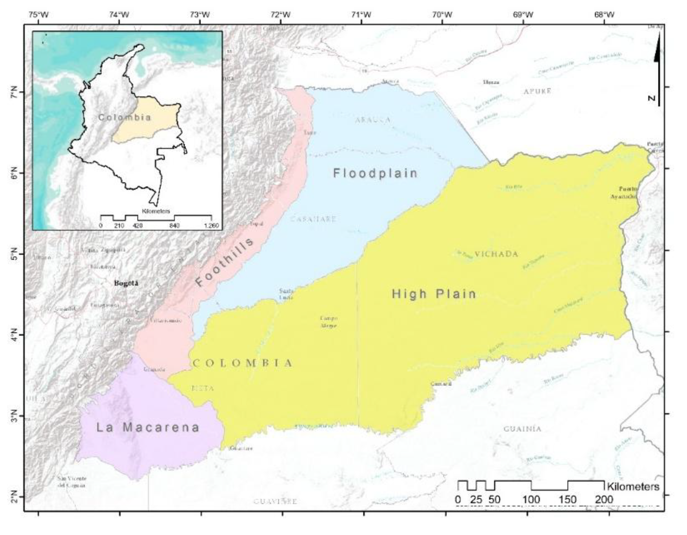
Figure 2.
Methodological and Cartographic Synopsis of Grasslands in the Colombian Orinoquia.
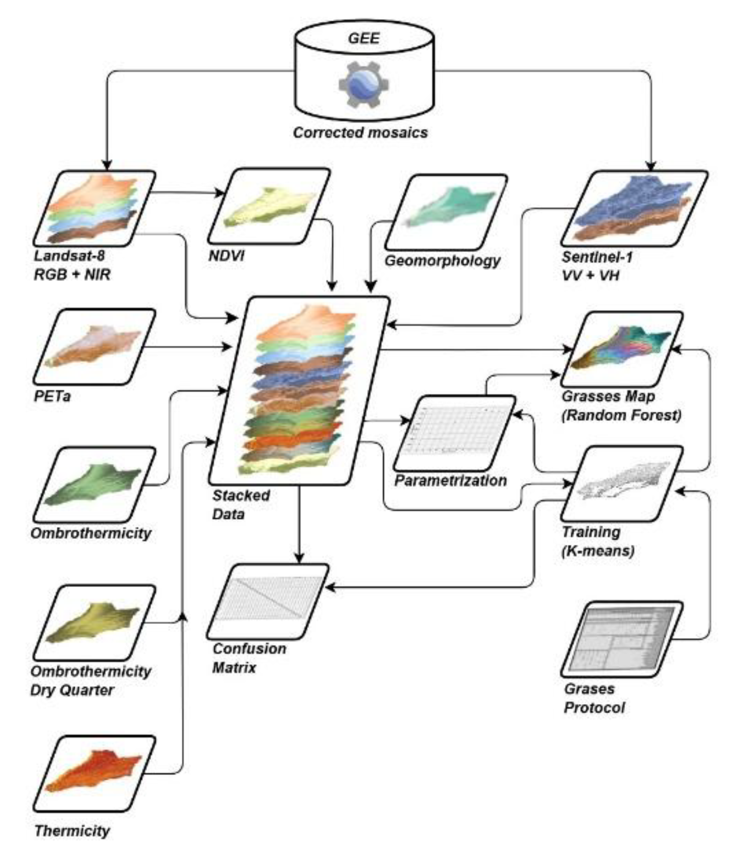
Figure 3.
Geographical distribution of Foothills Grasslands.
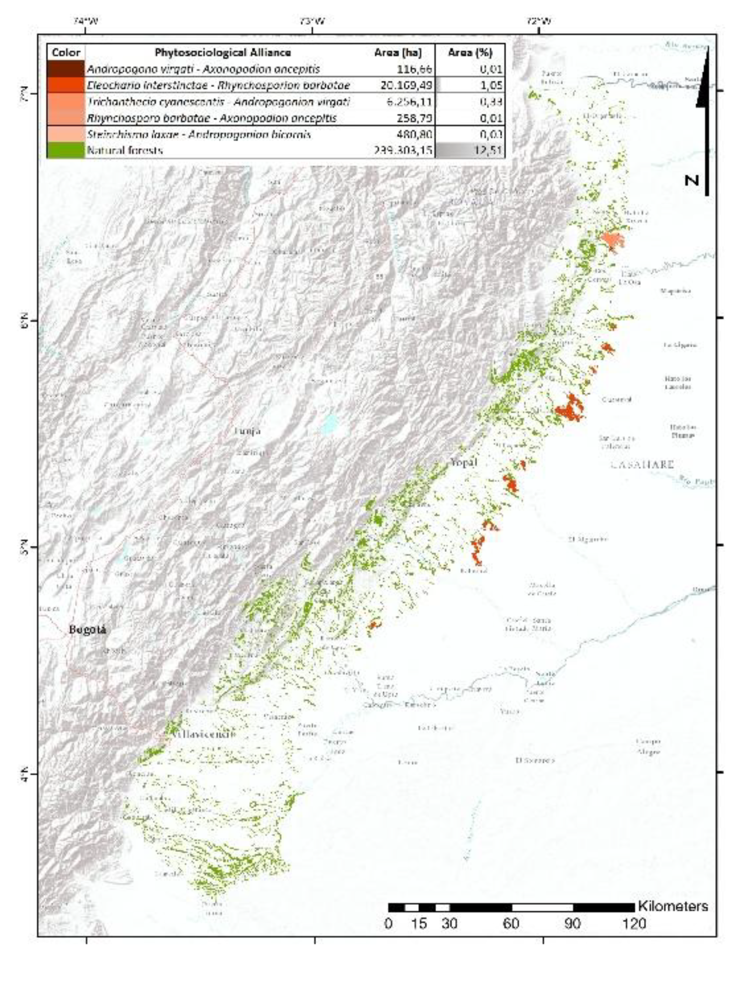
Figure 4.
Geographical distribution of La Macarena Grasslands.

Figure 5.
Geographical distribution of Floodplain Grasslands.
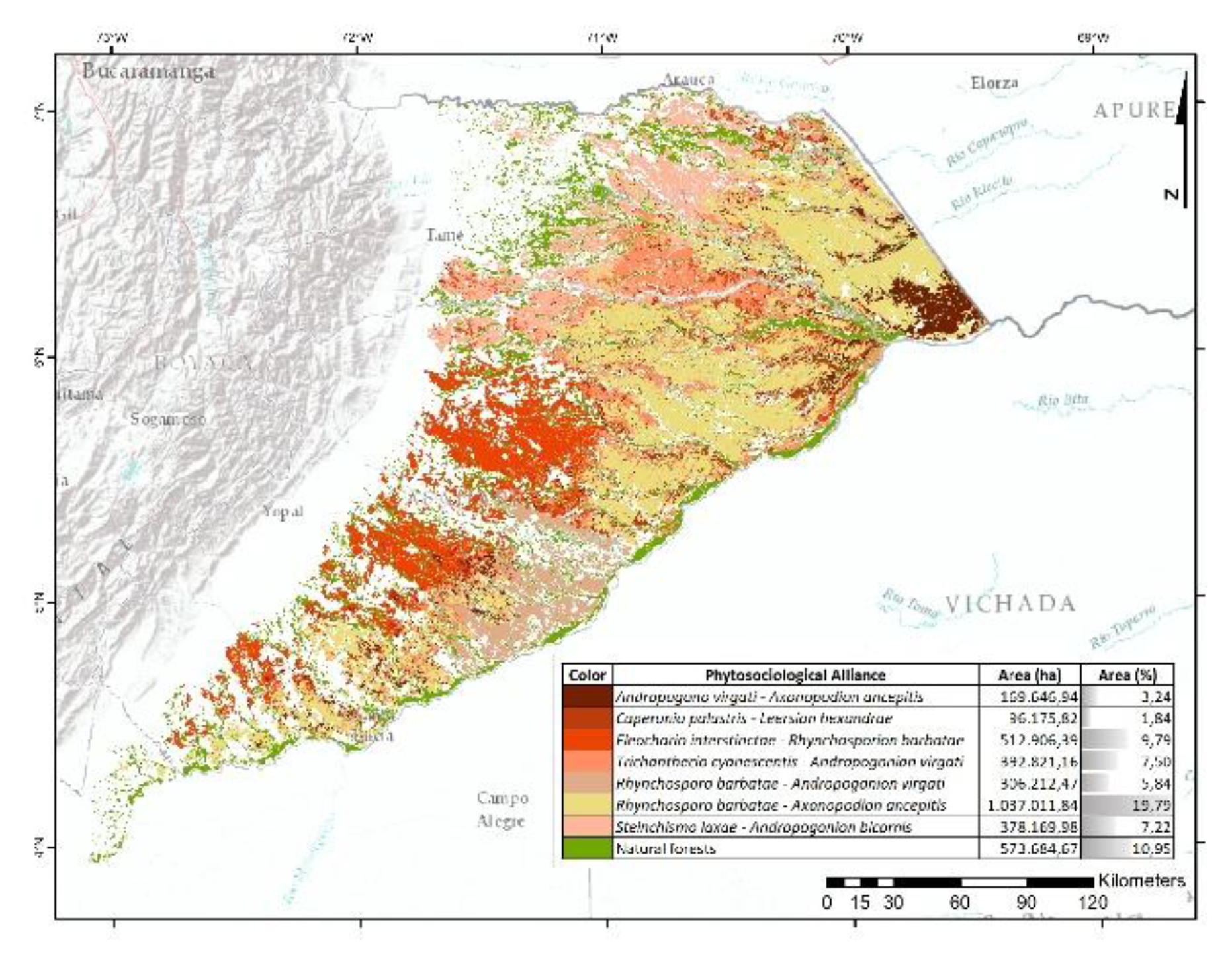
Figure 6.
Geographical distribution of High Plain Grasslands.
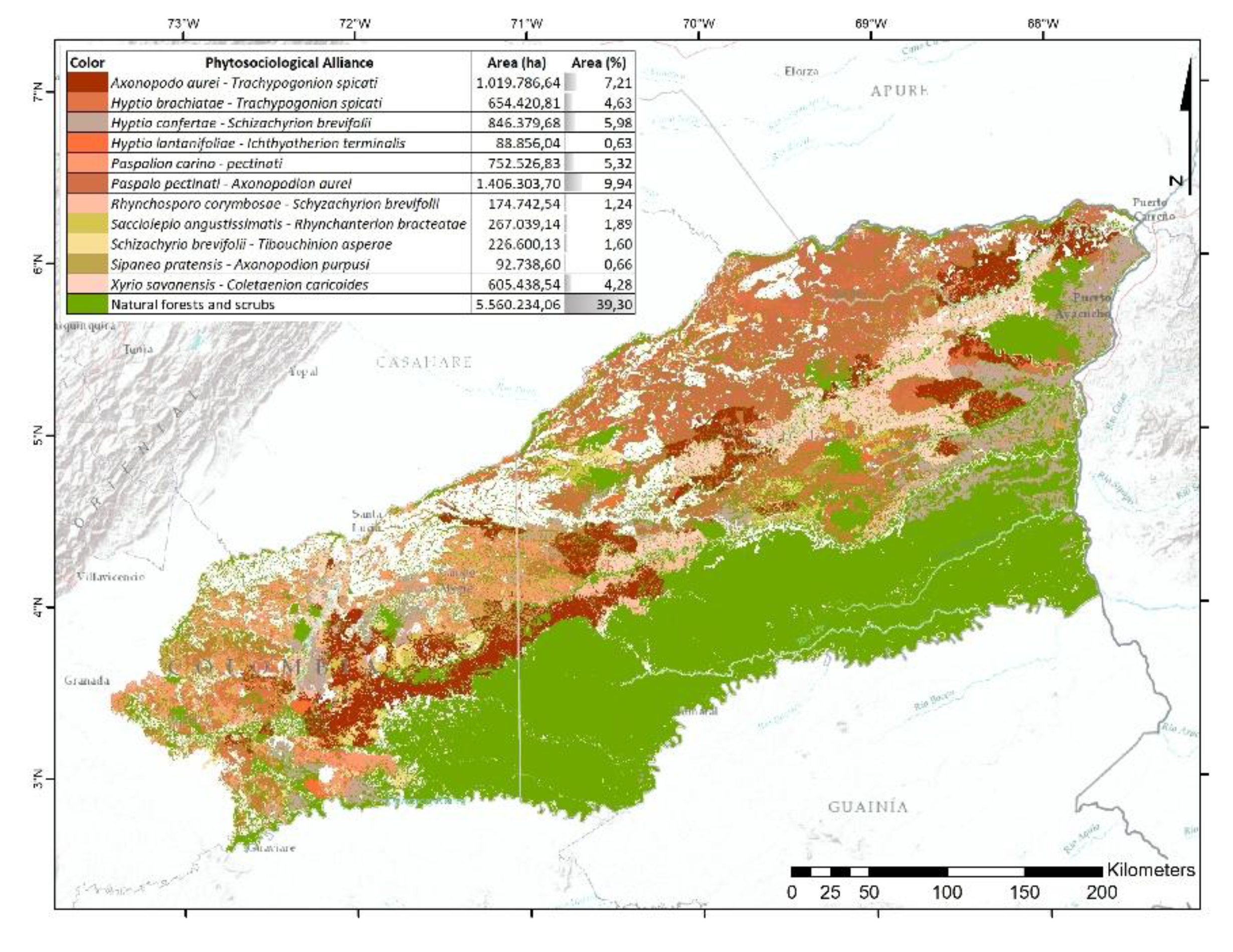

Table 1.
Area of the Orinoquia currently covered by natural grasslands.
| Phytosociological Alliance | Area (ha) | Area (%) |
|---|---|---|
| Axonopodo aurei - Trachypogonion spicati | 1,019,786.64 | 4.37 |
| Andropogono virgati - Axonopodion ancepitis | 169,763.59 | 0.73 |
| Caperonio palustris - Leersion hexandrae | 96,175.82 | 0.41 |
| Eleochario interstinctae - Rhynchosporion barbatae | 533,075.88 | 2.28 |
| Hyptio brachiatae - Trachypogonion spicati | 654,420.81 | 2.80 |
| Hyptio confertae - Schizachyrion brevifoli | 846,379.68 | 3.62 |
| Hyptio lantanifoliae - Ichthyotherion terminalis | 88,856.04 | 0.38 |
| Trichanthecio cyanescentis - Andropogonion virgati | 399,077.26 | 1.71 |
| Paspalion carino - pectinati | 833,054.74 | 3.57 |
| Paspalo pectinati - Axonopodion aurei | 1,406,303.70 | 6.02 |
| Rhynchosporo barbatae - Andropogonion virgati | 306,212.47 | 1.31 |
| Rhynchosporo barbatae - Axonopodion ancepitis | 1,037,270.63 | 4.44 |
| Rhynchosporo corymbosae - Schyzachyrion brevifolii | 174,742.54 | 0.75 |
| Sacciolepio angustissimatis - Rhynchanterion bracteatae | 267,039.14 | 1.14 |
| Schizachyrio brevifolii - Tibouchinion asperae | 226,600.13 | 0.97 |
| Sipaneo pratensis - Axonopodion purpussi | 92,738.60 | 0.40 |
| Steinchismo laxae - Andropogonion bicornis | 378,650.78 | 1.62 |
| Xyrio savanensis - Coletaenion caricoides | 605,438.54 | 2.59 |
Table 2.
With regard to the ecogeographical distribution of the syntaxa, none is common to all physiographic units, nor is any present in three of them. Thirteen phytocoenoses are distributed across two physiographic units. The most prominent axis of continuity is between the Foothills and Floodplain, followed by the High Plains–La Macarena regions, with seven and six alliances, respectively. The High Plains stands out for its singularity, with four alliances restricted exclusively to its territory.Table 2. Ecogeographical distribution, Dominance Ratio (DRi), and photosynthetic pathways (Poaceae) of grassland vegetation in the Colombian Orinoquia.
| Physiography | Phytosociological Alliance | spp. | Char. | DRi | Poaceaei | DRP | C3 | C4 | |
|---|---|---|---|---|---|---|---|---|---|
| Foothills-Floodplain | Andropogono virgati-Axonopodion ancepitis | 58 | 8 | 13,8 | 4 | 50 | 1 | 3 | |
| Foothills-Floodplain | Axonopodo aurei-Trachypogonion spicati | 46 | 8 | 17,4 | 3 | 37,5 | 0 | 3 | |
| Foothills-Floodplain | Caperonio palustris-Leersion hexandrae | 88 | 5 | 5,7 | 2 | 40,0 | 1 | 1 | |
| Foothills-Floodplain | Eleochario interstinctae-Rhynchosporion barbatae | 52 | 10 | 19,2 | 0 | 0,0 | 0 | 0 | |
| Highplain-La Macarena | Hyptio brachiatae–Trachypogonion spicati | 69 | 10 | 14,5 | 1 | 10,0 | 0 | 1 | |
| Highplain-La Macarena | Hyptio confertae-Schizachyrion brevifolii | 35 | 4 | 11,4 | 2 | 50,0 | 0 | 2 | |
| Highplain-La Macarena | Hyptio lantanifoliae–Ichthyotherion terminalis | 55 | 6 | 10,9 | 1 | 16,7 | 0 | 1 | |
| Highplain-La Macarena | Paspalion carino-pectinati | 63 | 17 | 27,0 | 3 | 17,6 | 0 | 3 | |
| Highplain-La Macarena | Paspalo pectinati-Axonopodion aurei | 36 | 4 | 11,1 | 3 | 75,0 | 0 | 3 | |
| Foothills-Floodplain | Rhynchosporo barbatae-Axonopodion ancepitis | 92 | 21 | 22,8 | 6 | 28,6 | 2 | 4 | |
| Highplain | Rhynchosporo corymbosae-Schyzachyrion brevifolii | 43 | 7 | 16,3 | 2 | 28,6 | 0 | 2 | |
| Floodplain | Rhynchosporo barbatae-Andropogonion virgati | 19 | 12 | 63,2 | 6 | 50,0 | 0 | 6 | |
| Highplain | Sacciolepio angustissimatis-Rhynchanterion bracteatae | 34 | 8 | 23,5 | 2 | 25,0 | 1 | 1 | |
| Highplain | Schizachyrio brevifolii-Tibouchinion asperae | 43 | 6 | 14,0 | 2 | 33,3 | 0 | 2 | |
| Highplains-La Macarena | Sipaneo pratensis-Axonopodion purpusi | 38 | 10 | 26,3 | 6 | 60,0 | 0 | 6 | |
| Foothills-Floodplain | Steinchismo laxae-Andropogonion bicornis | 62 | 5 | 8,1 | 3 | 60,0 | 1 | 2 | |
| Foothills-Floodplain | Trichanthecio cyanescentis-Andropogonion virgati | 87 | 8 | 9,2 | 4 | 50,0 | 1 | 3 | |
| Highplain | Xyrio savanensis-Coletaenion caricoides | 25 | 6 | 24,0 | 2 | 33,3 | 0 | 2 |
spp.: Number of species present in the alliance. Char.: Number of characteristic species within the alliance. DRi: Dominance Ratio of the characteristic species in the alliance. Poaceaei: Number of characteristic Poaceae species within the alliance. DRP: Dominance Ratio of Poaceae species relative to the total dominance of characteristic species from all other families in the alliance. C₃: Number of Poaceae species with a C₃ photosynthetic pathway in the alliance. C₄: Number of Poaceae species with a C₄ photosynthetic pathway in the alliance.
Disclaimer/Publisher’s Note: The statements, opinions and data contained in all publications are solely those of the individual author(s) and contributor(s) and not of MDPI and/or the editor(s). MDPI and/or the editor(s) disclaim responsibility for any injury to people or property resulting from any ideas, methods, instructions or products referred to in the content. |
© 2025 by the authors. Licensee MDPI, Basel, Switzerland. This article is an open access article distributed under the terms and conditions of the Creative Commons Attribution (CC BY) license (http://creativecommons.org/licenses/by/4.0/).
Copyright: This open access article is published under a Creative Commons CC BY 4.0 license, which permit the free download, distribution, and reuse, provided that the author and preprint are cited in any reuse.


