
Submitted:
28 December 2023
Posted:
03 January 2024
You are already at the latest version
Abstract
This study assesses the applicability of different-resolution multispectral remote sensing images for mapping and estimating the aboveground biomass (AGB) of Carpobrotus edulis, a prominent invasive species in European coastal areas. The performance of three sets of multispectral images with different resolutions was compared: (i) 2.5 cm Ground Sample Distance (GSD), 5 cm GSD and 10 cm GSD images. The images were classified using the supervised classification algorithm Random Forest and later improved applying a sieve filter. The results show that the three tested image resolutions allow constructing reliable coverage maps of C. edulis, with Overall Accuracy values of 89%, 85% and 88% for the classification of the 2.5 cm, 5 cm and 10 cm GSD images, respectively. Samples were also collected, dried and weighed to estimate AGB using the relationship between the Dry Weight and Vegetation Indices (VI). The regressions were evaluated based on their R² and Normalised RMSE. The best-performing VI-DW regression models achieved: R² = 0.87 and NRMSE = 0.09 for the 2.5 cm resolution; R² = 0.77 and NRMSE = 0.12 for the 5 cm resolution; and, R² = 0.64 and NRMSE = 0.15 for the 10 cm resolution. C. edulis area and total AGB were: 3441.10 m² and 28,327.1 kg (with a Relative Error (RE) = 0.08), for the 2.5 cm resolution; 3070.04 m² and 29,170.8 kg (RE = 0.08), for the 5 cm resolution; and, 2305.06 m² and 22,135.7 kg (RE = 0.11), for the 10 cm resolution. Differences were analysed in detail, spatially, to determine their causes. Final analyses suggest that, for C. edulis, multispectral imagery of up to 5 cm GSD is adequate for the estimation of the species’ distribution and biomass.
Keywords:
Carpobrotus edulis
; Unoccupied Aerial Vehicle
; Above-ground Biomass
; GIS
; QGIS
; Landcover Classification
1. Introduction
In the ever-evolving field of remote sensing (RS), the selection of the appropriate scale to investigate an object plays a central role in the accuracy and relevance of information, as geographical phenomena, distributions, and processes are generally scale-dependent [1]. As new sensors and platforms are developed through new technological advancements, from aeroplanes to drones as observation platforms, from panchromatic to hyperspectral sensors, an RS study overall effectiveness is still strongly related to its images’ Ground Sample Distance (GSD). There is, however, a trade-off between efficiency and accuracy, which are usually inversely proportional, with accuracy depending on image spatial and spectral resolutions, and with high resolutions liked to smaller areas.
Many studies use information from small areas, obtained with high-resolution sensors, to extrapolate the results to more extensive areas surveyed with lower-resolution sensors [2,3,4]. Even though good results can be achieved this way, these studies do not consider the scale effect, i.e. they do not address that, for a given area and object of study, there should be an optimum scale for monitoring [5].
Remote sensing techniques constitute a valuable tool for the management of invasive species. Unoccupied Aerial Systems (UAS) equipped with multispectral sensors have been increasingly used to identify and monitor different invasive species in many ecosystems, and their application can be considered a well-established technique [6,7,8,9]. Adding to that, multispectral UAS have also gained importance in commercial agriculture, where vegetation indices (VI) are used for crop health assessment and yield estimation [10,11,12,13]. Some recent studies of natural habitats have combined a species identification methodology with yield estimations to assess the vegetation’s Above-Ground Biomass (AGB) using multi- or hyperspectral UAS [14,15]. The measurement of AGB of invasive species can play a central role in the planning and execution of removal campaigns.
Original from South Africa, Carpobrotus edulis is a prominent invasive species in Europe, with its genus Carpobrotus, having the largest number of records of control actions in Mediterranean countries [16]. Remote-sensing methods are an obvious choice to facilitate its monitoring and management. This article examines three sets of multispectral images with different spatial resolutions, specifically focusing on the impact each resolution has on the estimation of C. edulis AGB. Data processing, classification algorithms, and the subsequent implications for AGB estimates accuracies were evaluated to gain insights into resolution impacts and improve decision making process on monitoring and removal campaigns.
2. Study Area
The study area was part of the Parque Natural do Litoral Norte (PNLN), administered by the national Nature and Forest Conservation Institute (Instituto da Conservação da Natureza e das Florestas – ICNF) (Figure 1). The park spreads along 16km of the coast, located between the Neiva estuary (41°36'46.56"N, 8°48'32.55"W) and the south border of Apúlia (41°28'10.68"N, 8°46'31.30"O), extending 5 km offshore into the ocean. It covers a total of 8887 ha, of which 7653 ha are marine areas.
The PNLN was created to protect the littoral of Esposende, preserve its natural resources and elements, and promote a rational use of the site. With its mainland consisting essentially of a strip of sandy shores, the park houses 15 different habitats described in the Habitat Directive, four of which being marked as priority habitats: 1150 - Coastal lagoons, 2130 - Fixed coastal dunes with herbaceous vegetation (grey dunes), 2270 - Wooded dunes with Pinus pinea and/or Pinus pinaster, and 91E0 - Alluvial forests with Alnus glutinosa and Fraxinus excelsior (Alno-Padion, Alnion incanae, Salicion albae).
Almost all in-land park terrain is located less than 10 m above mean sea level, with only some dunes between the 10 and 20 m high. There are 240 different vegetation species identified on the NLNP, most of them native to the north Iberic littoral, including some endangered species. This native vegetation is vital for preserving the morphological and biotic characteristics of the ecosystems [17]. However, like many other coastal environments, the dunes of the Cávado Estuary suffer not only from erosion risks but also from the constant pressure of climate change, urbanisation, recreation trampling and invasive species [18]. Twelve invasive species were identified within the flora, with the most prominent ones considered the Acacia longifolia and Carpobrotus edulis, which pose significant pressure on the dunar habitats [19].
3. Materials and Methods
This study was divided into four phases: In situ work (section 3.1), Laboratory Work (section 3.2), Imagery Processing (section 3.3), and C. edulis area and biomass estimation (section 3.4).
3.1. In Situ Work
The in-situ work was developed as follows: (i) marking of Ground Control Points, (ii) Placement of quadrats for sampling delimitation, and (iii) capture of aerial images.
Ground Control Points
Ground Control Points (GCP) were strategically distributed over the study area and marked with spray paint. These points were georeferenced with a GNSS receiver Emlid Reach M2 and a Novatel antenna (Novatel GPS-702-GG) in Real Time Kinematic (RTK) mode, with corrections from RENEP, the Portuguese CORS (Continuously Operating Reference Station) network, and later used to enhance the orthomosaic geometry and geolocation precision during imagery processing.
Sample quadrats
Thirty 50x50 cm² quadrats were placed over areas containing only C. edulis vegetation with different, visually identified biomass and health characteristics (Figure 2a). This distribution was designed to cover a range of conditions, with more or less lush plants and different biomasses per sample, to optimise the Dry Weight (DW) x Vegetation Indices (VI) regression models. The quadrats were also placed with a north-south orientation, which helps to reduce the number of pixels the frames occupy in the RS image and the number of neighbouring pixels affected by reflectance interference.
These quadrats have an essential role in identifying the sample areas; they are georeferenced with the GNSS receiver and, since they can be identified in the aerial images, they are used as visual marks for the samples.
Aerial images
Once the quadrats and ground control points were in place, marked and georeferenced, four different sets of aerial images were acquired using: a built-in RGB sensor from a DJI Phantom 4 to obtain images with 1 cm Ground Sample Distance (GSD); a five-band (R,G,B, RedEdg, NIR) Micasense RedEdge -MX sensor to obtain images with 2.5 cm GSD; and a four-band (R,G,B,NIR) Ultra Cam Falcon f100 M1 to obtain images with 5 and 10 cm GSD.
The RGB camera from the DJI Phantom 4 UAV was only used to provide a very high-resolution RGB orthomosaic to allow a reliable cover identification. The other three sets of images were processed to assess their capability to identify and estimate the AGB of C. edulis.
To avoid the effect of the reflectance interference of the quadrat frames on the VI of the sample areas, only the central part of the quadrats was sampled and analysed. Therefore, after the aerial survey, all the AGB within the central 30x30 cm² of each of the 30 quadrats was collected, bagged, tagged and taken to the lab for biomass determination. To do so, the smaller quadrat was visually positioned in the centre of the 50x50 cm² quadrat, as shown in Figure 2b, and the AGB was cut out with a saw and scissors. After AGB collection, the samples were taken to the lab and processed.
3.2. Laboratory Work
It is essential to address that Carpobrotus edulis has the characteristic of growing in two distinct layers, an upper layer – which absorbs and reflects the sunlight and is visible in the aerial images – and a lower layer composed of older and dryer stems and leaves that are generally not visible from above. The two layers of the collected plant material were therefore separated and weighted separately on a scale to the nearest 0.01g to obtain the wet weight (WW) of each layer for each sample.
After weighing, green and brown parts were placed in the lab stove at 60°C to be dried, being weighed daily until they presented no weight difference between two consecutive weightings. After drying, all samples were weighted on the same scale to the nearest 0.01g. The DW was later used to (i) relate biomass with VIs (section 3.2), (ii) compare DW and WW, and (iii) assess the biomass ratio between the green and brown parts of the plants.
3.3. Image Processing and Analyses
Each set of images, with 2.5, 5 and 10 cm GSD, respectively, was processed according to the following steps: (i) orthomosaic production, (ii) Vegetation Indices calculation and DW-VI empirical modelling for AGB estimation, and (iii) land cover classification, accuracy assessment and error analysis.
Orthomosaics
RGB and multispectral orthomosaics were computed with Agisoft Metashape Professional version 1.8.3 built 14331 (64bit), using the georeferenced sample quadrats and GCP for image orthorectification.
Vegetation Indices and Biomass
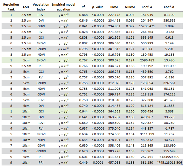
AGB was estimated based on the relationship between vegetation DW and VI derived from the image bands. Based on a previous study, where sixteen VI were evaluated for their ability to estimate the AGB of C. edulis [20], the best performing VI (with DW-VI model R² ≥ 0.75) (Table 1) were selected to compare the performances of the different spatial resolution images in estimating C. edulis AGB. The indices were computed using the QGIS 3.28.3 raster calculator tool, creating VI maps for the study area.
Mean VI values were computed for each AGB sample collection area. Notice that the pixels used coincided with the 30x30 cm collection area square in the centre of the 50x50 quadrats. The obtained VI values were later used to assess their relationship with the sample DW of the plants’ green parts
Each sample’s DW of the green parts (y-axis) was plotted against the mean VI (x-axis) to evaluate the relationship between the two parameters. One linear and three exponential regression models were evaluated to select the best fitting model for each VI and image resolution:
where:
| Linear model (lin) (1) |
| Exponential model 1 (xpo1) (2) |
| Exponential model 2 (xpo2) (3) |
| Exponential model 3 (xpo3) (4) |
Dry Weight
Vegetation Index
coefficient 1
coefficient 2
Only the green parts DW was used because of the limitations of the aerial images, which only capture the reflectance of the top layer of C. edulis. The best fitting regression model was selected based on the R², p-value and a Normalised Root Mean Square Error (NRMSE), calculated dividing the RMSE by the difference between maximum and minimum observed DW of green parts.
Cover Classification
The orthomosaics were classified through a supervised classification with the random forest algorithm. The random forest algorithm, was selected based of its performance in previous studies on identifying C. edulis [20].
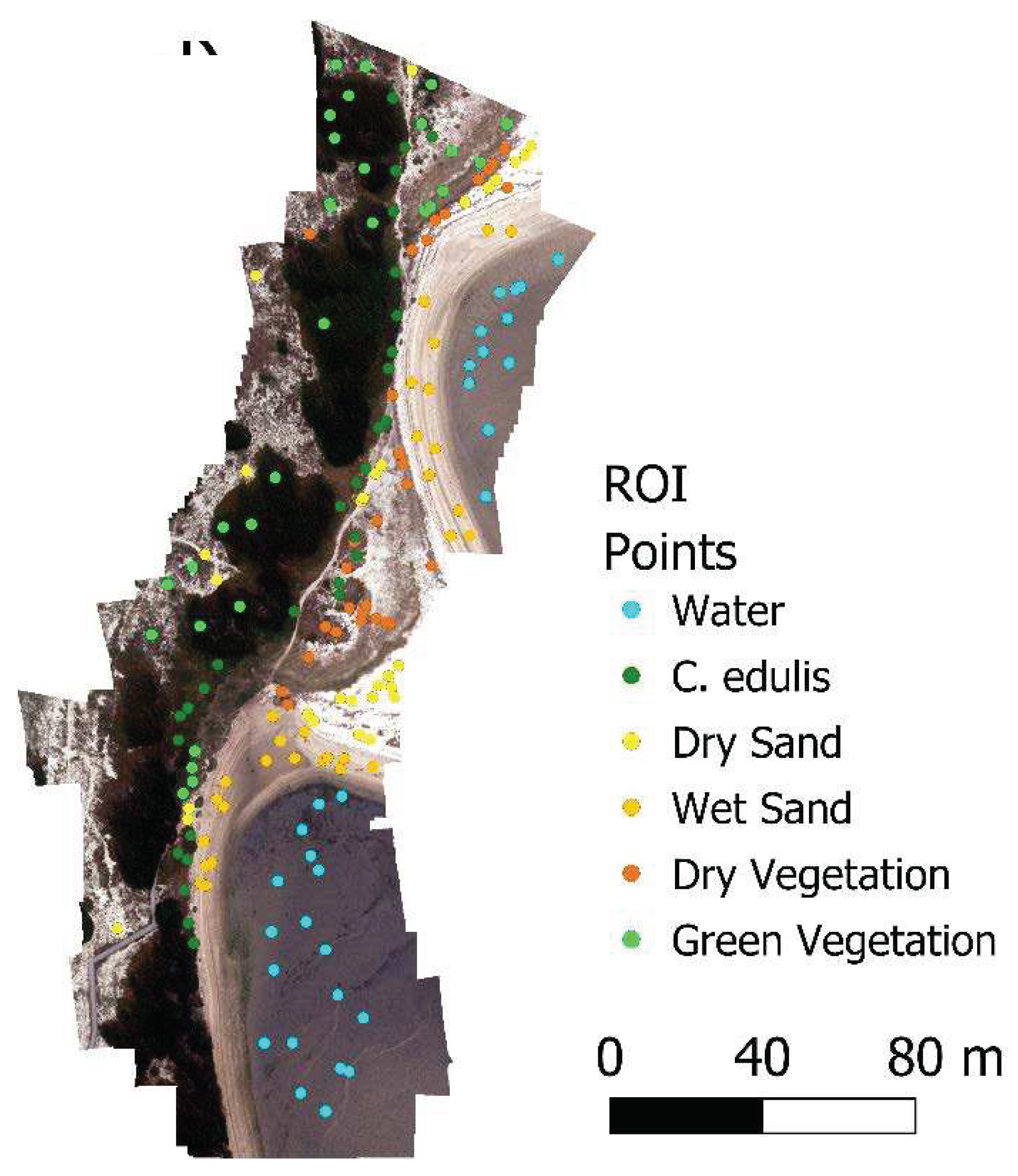
The number of cover classes was determined by visual identification of the most relevant covers in the image, and 30 Regions Of Interest (ROI) of 20x20 cm were selected for each class for the training of the classification, resulting in approximately 13,000 pixels. For the target C. edulis class, the ROIs were created near to the vegetation sampling areas (Figure 3).
Figure 3.
Othomosaic image with 10cm GSD and ROI points marked.
The number of ROI for the different spatial resolutions was defined to approximate 13,000 training pixels (Table 2), a number of pixels that resulted in a satisfactory classification in the previous study [20].

Table 2.
ROIs and training pixels count per resolution.
| GSD (cm) | Individual ROI area (cm) | Pixels per ROI | Number of ROIs per class | Total training pixel count |
|---|---|---|---|---|
| 2.5 | 20 x 20 | 64 – 81 | 30 | 13,269 |
| 5.0 | 20 x 20 | 16 | 120 | 11,520 |
| 10.0 | 20 x 20 | 4 | 460 | 11,524 |
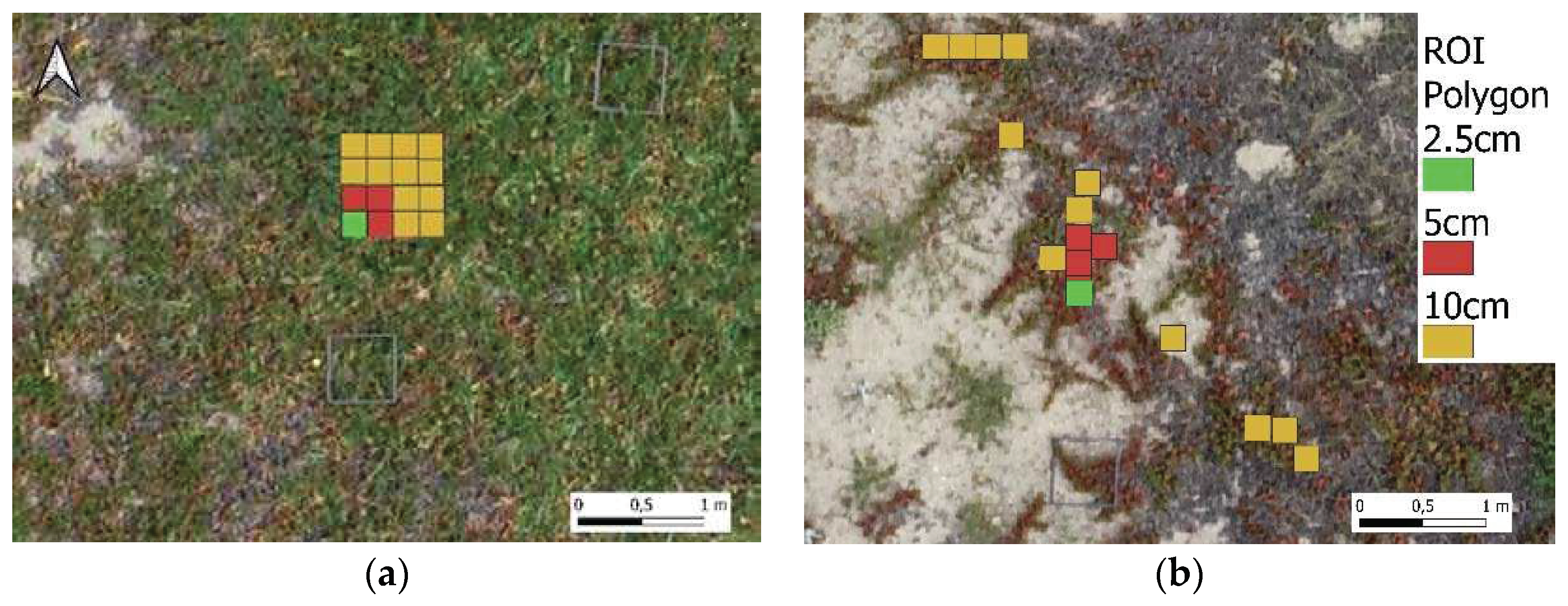
For the lower-resolution orthomosaics, the ROI were positioned as close as possible to the ROI of the 2.5 cm GSD orthomosaic. Notice that the ROI of 2.5 cm is also part of the ROI of 5 cm, which, in turn, is also part of the ROI for the 10 cm GSD orthostatic (Figure 4). Examples of ROI distribution are provided in Figure 4 a) and b), showing 1 ROI for 2.5 cm GSD, 4 ROIs for 5 cm GSD, and 16 ROIs for 10 cm GSD, in order to achieve approximately similar numbers of training pixels.
Figure 4.
ROI for C. edulis when located over a homogeneous area (a), and located over a non-homogeneous area (b).
Figure 4.
ROI for C. edulis when located over a homogeneous area (a), and located over a non-homogeneous area (b).
The accuracy of each classification was assessed based on a large set of randomly selected pixels, from which the ground truth cover class was visually identified in the 1 cm GSD RGB image and compared to the classified class. The number of pixels for the accuracy test was defined based on the proportion of each class and the expected standard deviation of each class [30] according to the following equation.
where:
total number of pixels
mapped area proportion of class I;
standard deviation of stratum I;
expected standard deviation of overall accuracy;
The classifications were evaluated in terms of the F1 score of the C. edulis cover class, i.e. considering a harmonic mean between User Accuracy (UA) and Producer Accuracy (PA).
Sieve filters with progressive strength were applied, using QGIS (3.28), to reduce the number of small patches of possibly incorrectly classified pixels (considered noise), aiming to improve accuracy. Two types of sieve filters were used: a 4-pixel filter, which only considers the pixels on the edges of the target pixel as neighbour pixel; and an 8-pixel filter, which considers all pixels connected to the edges and corners of the target pixel as neighbours. The two filters were used with progressively larger thresholds (i.e. larger areas used to re-calculate the pixel(s)’ class) doubling at every interaction (1, 2, 4, 8, 16, (…), 2048) until the accuracy of the classification stopped increasing and started to fall. The increase in the accuracy with increasing threshold can be linked to classification noise reduction, but as the filter becomes larger, the classification begins to lose information, reducing its accuracy.
3.4. C. edulis Area and Biomass Estimation
For each image resolution, the land cover classification with the highest F1 score was used to obtain the total area of C. edulis (Figure 5).
To estimate the total C. edulis biomass for the classified area, the following information is necessary, (i) C. edulis classified area; (ii) pixel VI values in the C. edulis area; (iii) the regression model correlating the VI value with the DW of the green parts of C. edulis; (iv) the relation between the DW and WW; and (v) the ratio between the WW of green and brown parts.
For the biomass estimation, the pixel VI values were converted to AGB DW using the best-fitting regression model. This allowed calculation of the green-part DW of each pixel classified as C. edulis. After that, the DW was converted to WW, using the previously established WW-DW relationship. Finally, to assess the total weight of C. edulis in the study area, an estimate of the brown-part AGB had to be added, since only the green parts have been accounted for in the regression model. This was achieved using the ratio between the WW of green and brown parts.
There are different errors to be considered using the proposed methodology: (i) geometric distortions, which depend on sensor perspective and motion, platform stability, terrain relief and the curvature and rotation of the earth (less relevant for small surveyed areas); (ii) sensor errors, causing image deformation; (iii) Classification errors; (iv) Regression model errors; (v) the natural variability of the relationship between DW and WW, largely dependent on environmental conditions and plant moisture, which can produce AGB estimation errors; and (vi) the variability in the ratio between green and brown parts, which will depend on the age and development of the vegetation, also contributing to AGB estimation errors. For this study, only the (iii) classification and (iv) regression errors were considered in the final AGB estimation. The classification error (expressed in m²) is directly related to the accuracy evaluation procedure, from which an area Standard Error (SE) and a 95% Confidence Interval (CI) can be extracted. The RMSE (kg/m²) was extracted from the regression model and also considered in the total AGB estimation. The two errors were added for a conservative evaluation of the methodology. Further discussion can be found in section 4.2.
4. Results
4.1. Image Classification Results
Cover Classification
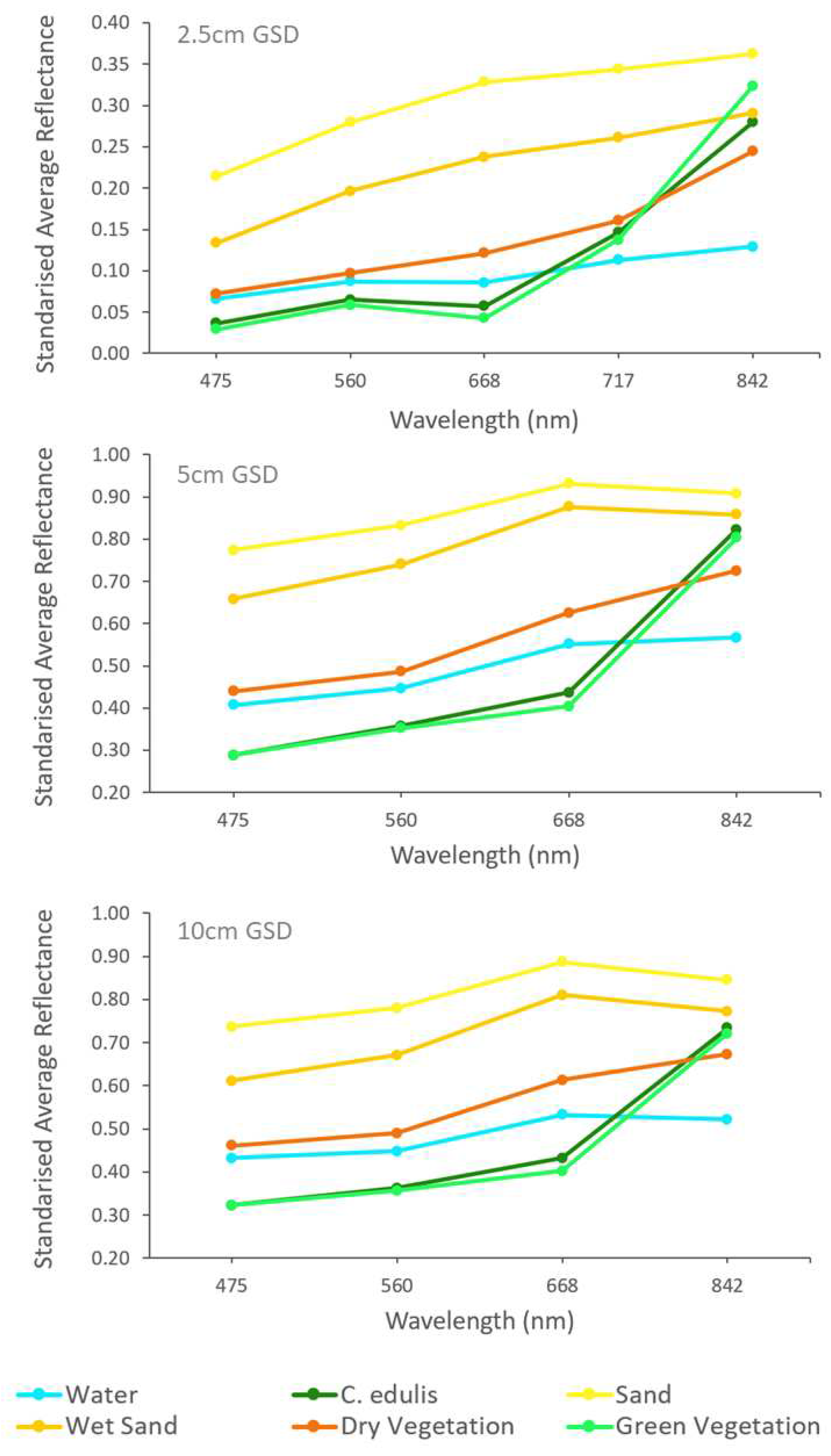
Six most relevant covers could be identified in the orthomosaic: Water, C. edulis, Sand, Wet Sand, Dry Vegetation and Green Vegetation. The Dry Vegetation and Green Vegetation classes included all vegetation species in the study area that were not identified as C. edulis. The mean spectral signatures of the ROI training areas for each class and for the different image resolutions are displayed in figure 6.
Classification Accuracy Assessment
Applying Equation (v) for every classification resolution, while accounting for a class-specific standard deviation of 0.3 and an overall accuracy standard deviation of 0.01, resulted in an accuracy assessment using 780 pixels. An equal distribution was applied with 130 randomly generated pixels for each class, aiming to enhance the reliability of accuracy for C. edulis cover class. The first accuracy assessment presented the following results: 2.5 cm GSD – C. edulis F1 score 72.6 an OA 85.9; 5cm GSD - F1 score 70.6 and OA 87.1; 10 cm GSD – F1 score 75.5 and OA 87.2.
Sieve Filter Effects
When applying the sieve filter, the different resolution classifications presented overall similar behaviour (Figure 8). In general, as the filter threshold increased, the F1 Score for C. edulis increased, while the classification noise decreased, until it dropped significantly, when too much information was lost. This happened at different thresholds for the different imagery resolutions.
Figure 6.
Mean spectral signatures of ROI divided by class and GSD orthomosaic.
The different resolution images resulted in classifications with different cover class distributions (Figure 7), with varying proportions, particularly for the of target class C. edulis and for green vegetation.
Figure 7.
Cover class distribution for the classification results obtained with each spatial resolution.
Figure 7.
Cover class distribution for the classification results obtained with each spatial resolution.
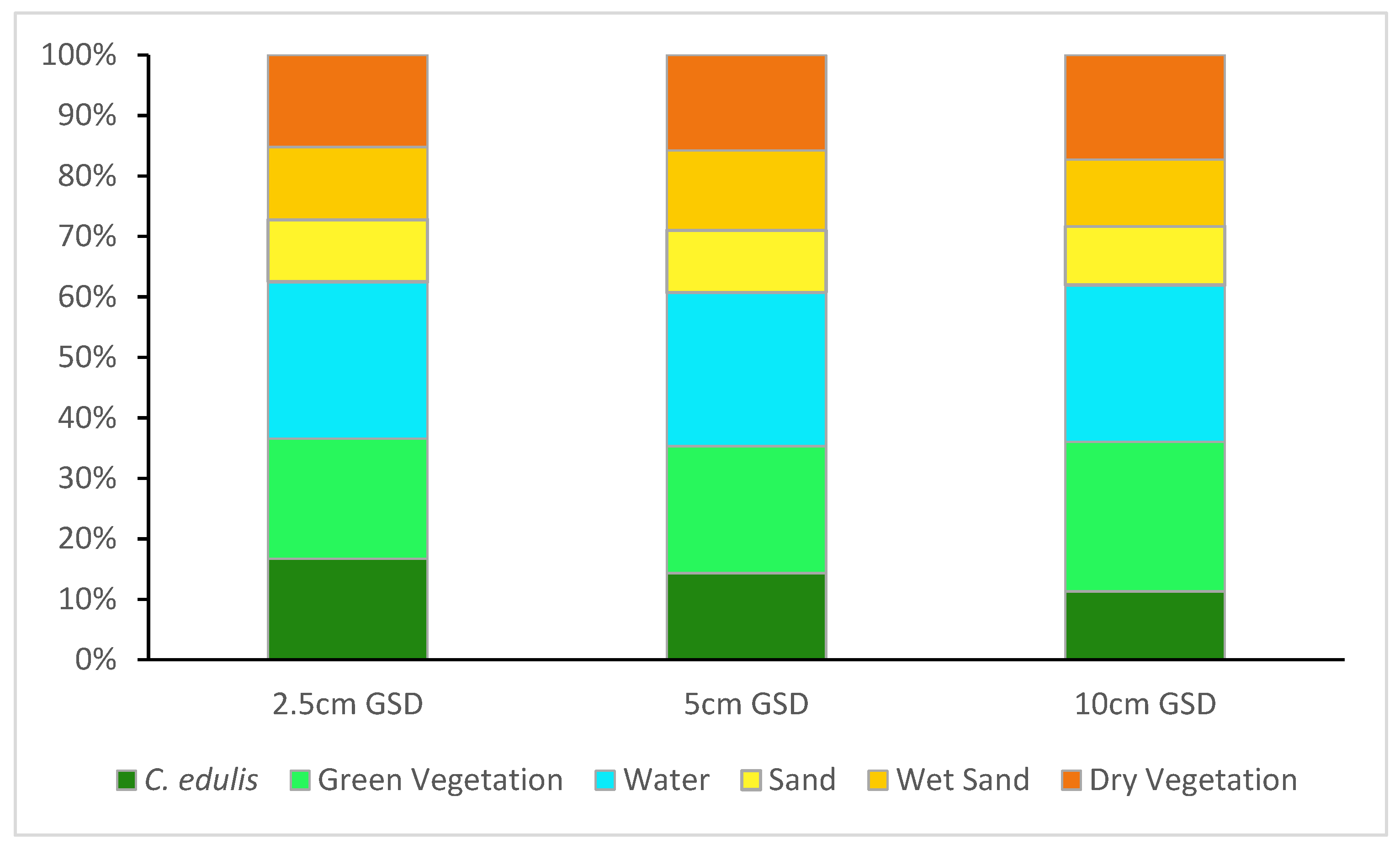
Figure 8.
Comparison of F1 Score for the C. edulis class for different filters (4: 4-pixel filter; 8: 8-pixel filter), thresholds and resolutions. Highest F1 score marked in red.
Figure 8.
Comparison of F1 Score for the C. edulis class for different filters (4: 4-pixel filter; 8: 8-pixel filter), thresholds and resolutions. Highest F1 score marked in red.
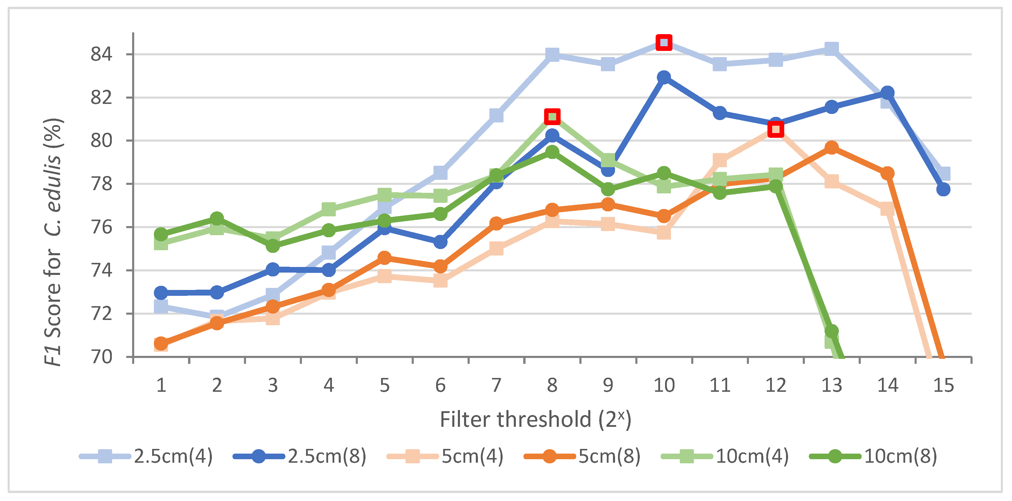
The sieve filter that achieved the highest F1 Score for C. edulis for each survey resolution (identified in Figure 8), was used for the C. edulis area estimation. Given that C. edulis is the target species and its class accuracy is the central object in the present study, the F1 Score was the only criterion considered for the sieve filters selection. However, the overall accuracy (OA) was still relevant and was also analysed.
For 2.5 and 10 cm GSD, the classifications’ OA increased by 4.4% and 1.4% respectively, if compared with the classification with no filter applied. The 5 cm GSD classification presented a 1.8% decline of its OA, but the F1 Score for C. edulis increased 9.9%, which justified the use of the filter.
The best results in terms of F1 scores for all resolutions were achieved using the sieve filter with a connectedness of 4 pixels. However, the threshold was different for every resolution, and each classification resulted in a different final classified C. edulis area (Table 5). A complete area-based classification error matrix of each resolution can be found in Appendix A (Table A1 to A3).
4.2. Biomass Estimation
The samples’ wet and dry weights for the green and brown parts of the collected C. edulis AGB are presented in Table 3. Notice that some samples did not present any brown plant parts.
To estimate the proportions of the WW of the Green (WWgreen) and Brown (WWbrown) plant parts, a simple mean ratio was calculated using all the samples, WWgreen/WWbrown = 15.9. The relationship between the WW and DW of the Green parts resulted in a mean ratio WWgreen/DWgreen = 7.0. The mean ratio considered the mean of the ratio between WWgreen/DWgreen of each sample area.
The best model for the relationship between the sample’s DWgreen and the sample area mean VI values, obtained for each image resolution, are presented in Table 4. All DWgreen—VI regressions were significant (p-value < 0.001). Plots of the best performing empirical regression models can be found in Appendix A (Figure A1 to A3).
Different indices performed best for the different resolution images. The best-performing VI was the Renormalized Difference Vegetation Index (RDVI) for 2.5cm GSD, the Enhanced Normalized Difference Vegetation Index (ENDVI) for 5cm GSD, and the Green Chlorophyll Index (GCI) for 10 cm GSD. These indices were therefore applied to estimate the total biomass of C. edulis in the study area, computing the DWgreen for all pixels classified as C. edulis. Notice that, even though these were the best-performing indices, many of the other indices tested also presented a satisfactory performance. Seven of eight other indices from the 2.5 GSD images presented an R² that was less than 10% lower than the R2 of the best performing index. Likewise, seven of the eight other indices applied to the 5 and 10 cm GSD images presented R² values that were less than 5 % lower than that of the best VI. A complete table with the best-performing regression models for each VI can be found in Appendix A – Table A4.
Notice that, even though the classification accuracy did not decrease much with the increase of the GSD (i.e. decrease in image resolution), the coefficient of determination R2 of the regression model significantly decreased with increasing GSD (Table 5). This is probably due to the amount of information available in the sample areas. For the 2.5 cm GSD there are up to 144 pixels in each sample area, while for 5 and 10 cm GSD there are only 36 and 9 pixels, respectively. The lower amount of information will reduce the efficiency of the regression models.
For each image resolution, C. edulis green-part DW was calculated applying the regression models to the classified area of C. edulis. The resulting values were subsequently converted to WWgreen, using the above-mentioned WW/DW ratio of 7.0. Finally, the area's total AGB of C. edulis was estimated using the WWgreen/WWbrown ratio of 15.9, resulting in values of total AGB for each classification (Table 5).
Table 5.
Classification results, AGB values and Total AGB estimates, considering the classified and estimated areas.
Table 5.
Classification results, AGB values and Total AGB estimates, considering the classified and estimated areas.
| Image resolution | ||||
|---|---|---|---|---|
| 2.5 cm | 5 cm | 10 cm | ||
| Classification | Filter Threshold | 1024 | 4096 | 256 |
| C. edulis Classified Area (m²) | 3441 | 3070 | 2305 | |
| F1 Score C. edulis | 84.5 | 80.5 | 81.1 | |
| Overall Accuracy | 89.5% | 85.3% | 88.6% | |
| Kappa hat | 0.871 | 0.808 | 0.859 | |
| C. edulis Estimated area (m²) | 2982 | 2616 | 2431 | |
| Standard Error of estimated area (m²) | 176 | 160 | 160 | |
| 95% confidence Interval estimated area (m²) | 345 | 314 | 313 | |
|
AGB values (WW) Based on VI empirical models |
RMSE (kg/m²) | 0.23 | 0.30 | 0.36 |
| Highest Value (kg/m²) | 29.13 | 29.18 | 24.50 | |
| Lowest Value (kg/m²) | 1.23 | 1.80 | 3.58 | |
| Mean (kg/m²) | 8.23 | 9.50 | 9.60 | |
| Median (kg/m²) | 7.67 | 9.44 | 9.41 | |
| Standard Deviation (kg/m²) | 3.66 | 3.16 | 2.88 | |
| Total AGB classified area | Total AGB (kg) | 28,327 | 29,170 | 22,135 |
| Regression model error (RMSE * Classified area) (kg) | 782 | 923 | 840 | |
| Classified area error (kg) | 1449 | 1520 | 1537 | |
| Total AGB error (kg) | 2231 | 2443 | 2377 | |
| Relative error | 0.08 | 0.08 | 0.11 | |
| Total AGB Estimated area | Total AGB (kg) | 24,548 | 24,857 | 23,345 |
| Total AGB error (kg) | 2231 | 2443 | 2377 | |
| 95% CI AGB error (kg) | 3518 | 3770 | 3892 | |
| Fractional error (Total AGB error) | 0.09 | 0.10 | 0.10 | |
| Fractional error (95% CI AGB error) | 0.14 | 0.15 | 0.17 | |
In terms of error analysis, the regression model error and the classification error were estimated. The regression error considered the root mean square error of the model, the RMSE (kg/m²), which was multiplied by the total classified area, resulting in an error in kg for the total AGB. The classification error was based on the estimated classified area's Standard Error (SE). A more detailed explanation of the estimated area and its SE can be found in section 4.4 of Olofsson et al. (2014)[30]. Even though the SE is related to the estimated reference area, it is intrinsically linked to the accuracy of the classification. The SE was multiplied by the mean value of AGB to estimate the total error of classified area (Table 5).
5. Discussion
5.1. Image Classification
The present study assessed the cover of the invasive species C. edulis through land cover classification of multispectral imagery (orthomosaics) of different resolutions. The supervised random-forest classification presented satisfactory results in identifying C. edulis (Table 5) for all three analysed resolutions, if compared to similar studies [33,34,35]. However, despite the satisfactory accuracies, the areas classified as C. edulis varied considerably in size. The difference was more prominent for the 10cm GSD image classification, which estimated C. edulis area was 33% and 25% less than the area estimated for the 2.5 cm GSD and the 5 cm GSD image classifications, respectively.
Examination of Table 5 (Classification) indicates that some aspects deserve further investigation, in order to: (i) determine where the differences in the area of C. edulis between classifications occur; (ii) identify the different attributed classes for the different resolutions and investigate the possible reasons for these differences; (iii) assess if the reference raster estimated area can be utilised with the mean vegetation values to estimate total AGB, considering that the estimated C. edulis areas for the reference rasters for all three resolutions were within the 95% confidence intervals of each other.
Notice that, even though all resolutions presented some relevant results, the total biomass of C. edulis obtained from the 2.5 cm GSD images captured by the MicaSense RedEdge-MX was considered the most accurate. This was justified by the higher image spatial resolution, and thus more detailed information available, by the higher number of bands available for classification (5 bands as opposed to the 4 bands from the lower resolution images), which provided more spectral information, probably resulting in better classification results, and the better DW-VI regression model results, which increase the confidence in the total AGB estimation.
To better understand the marked differences between resolutions in the areas classified as C. edulis , the classifications were compared in detail (Tables 6 to 8). A representative area of the orthomosaics cover changes is presented in Figure 9. The comparison between the 2.5 GSD classification and the other imagery classifications showed that the changes from smaller to larger GSD are characterised by the reduction of C. edulis classified cover area (Table 5), replaced mainly by Green and Dry Vegetation. These changes occur in small patches, close to the border of C. edulis areas and inside bigger C. edulis areas (Figure 9). The observed differences may be due to a scale effect of the resolution, an imprecision in the superposition of orthomosaics, a miss-classification due to overlapping spectral signatures or a mixture of these effects. The scale effect can be defined as the influence of spatial resolution on classification accuracy [36].
The different cover classes observed at the border of the C. edulis areas might be attributed to imprecision in the superposition of orthomosaics and to the scale effect. These effects are more relevant at the border of classified cover areas, where the reflectance of C. edulis areas may mix with the reflectance of neighbouring covers due to the larger GSD. As seen in Figure 9, some of these changes are at the border between C. edulis and Green Vegetation cover, which are the two classes with the less distinct spectral signatures. It is also interesting to notice that these differences are distributed on all sides of C. edulis borders, suggesting that these changes cannot be explained by orthomosaic superposition imprecisions alone (as these would produce a lateral shift). Some changes are also on the border between C. edulis and dry sand, where C. edulis pixels (according to the 2.5 cm classification) were classified as green vegetation, also likely due to the scale effect and spectral signature inaccuracy in larger pixels, which are more likely to display mixed cover than smaller pixels.
Larger areas of cover change, especially in the central part of C. edulis classified areas, cannot be explained by superposition imprecision or by the scale effect. These changes are probably related to misclassifications due to overlapping spectral signatures. Figure 6 shows that even though there was sufficient differentiation between the spectral signature of Green Vegetation and of C. edulis to provide a satisfactory classification accuracy, a considerable overlapping of theses signatures must be acknowledged. This overlapping might result in uncertainties and miss classification of C. edulis and Green Vegetation covers.
Mis-classifications may further be accentuated by the lack of the RedEdge band in the plane-based aerial photographs, i.e. the 5 and 10 cm GSD images. Analysing the pairwise comparisons (Tables 6 to 8) it is possible to see that most cover changes occurred between C. edulis and Green Vegetation, which may point to an inaccuracy related to the lower spectral resolutions from the 5 and 10 cm GSD. The extra RedEdge band of the UAS camera seems to provide some additional information that enhances classification accuracy.
A further and deeper investigation may allow identification of the most significant factors influencing cover discrepancies between resolutions in larger areas. An analysis of the classification confidence map for these areas may provide some helpful information.
Table 6.
Comparison of the cover class areas resulting from the 2.5 and 5 cm GSD classifications.
| 5 cm GSD | ||||||||
|---|---|---|---|---|---|---|---|---|
| Water | C. edulis | Dry Sand | Wet Sand | Dry Vegetation | Green Vegetation | Total 2.5cm GSD Area (m²) | ||
| 2.5 cm GSD | Water | 5555 | 3 | 2 | 103 | 298 | 16 | 5979 |
| C. edulis | 0 | 2548 | 9 | 6 | 300 | 574 | 3440 | |
| Dry Sand | 80 | 15 | 1685 | 26 | 504 | 16 | 2328 | |
| Wet Sand | 37 | 9 | 88 | 2349 | 45 | 0 | 2532 | |
| Dry Vegetation | 23 | 143 | 327 | 131 | 3274 | 197 | 4098 | |
| Green Vegetation | 4 | 349 | 23 | 8 | 225 | 3609 | 4221 | |
| Total 5cm GSD area (m²) | 5701 | 3069 | 2138 | 2627 | 4649 | 4416 | 22602 | |
Table 7.
Comparison of the cover class areas resulting from the 5 and 10 cm GSD classifications.
| 10 cm GSD | ||||||||
| Water | C. edulis | Dry Sand | Wet Sand | Dry Vegetation | Green Vegetation | Total 5cm GSD Area (m²) | ||
| 5 cm GSD | Water | 5604 | 0 | 0 | 14 | 85 | 0 | 5704 |
| C. edulis | 1 | 2029 | 5 | 0 | 84 | 946 | 3069 | |
| Dry Sand | 0 | 9 | 1774 | 76 | 263 | 13 | 2138 | |
| Wet Sand | 83 | 10 | 13 | 2187 | 324 | 8 | 2627 | |
| Dry Vegetation | 41 | 79 | 295 | 8 | 3654 | 565 | 4645 | |
| Green Vegetation | 66 | 175 | 6 | 0 | 96 | 4069 | 4413 | |
| Total 10 cm GSD area (m²) | 5798 | 2304 | 2095 | 2287 | 4509 | 5603 | 22599 | |
Table 8.
Comparison of the cover class areas resulting from the 2.5 and 10 cm GSD classifications.
| 10 cm GSD | ||||||||
| Water | C. edulis | Dry Sand | Wet Sand | Dry Vegetation | Green Vegetation | Total 2.5cm GSD Area (m²) | ||
| 2.5 cm GSD | Water | 5564 | 0 | 5 | 30 | 367 | 11 | 5979 |
| C. edulis | 10 | 2075 | 14 | 0 | 143 | 1194 | 3438 | |
| Dry Sand | 80 | 15 | 1772 | 32 | 414 | 12 | 2327 | |
| Wet Sand | 53 | 8 | 36 | 2172 | 256 | 6 | 2532 | |
| Dry Vegetation | 33 | 87 | 252 | 48 | 3204 | 468 | 4093 | |
| Green Vegetation | 52 | 118 | 14 | 3 | 122 | 3909 | 4219 | |
| Total 10 cm GSD area (m²) | 5794 | 2304 | 2094 | 2287 | 4508 | 5602 | 22592 | |
5.2. Biomass Estimation
For the quantification of vegetation through regression models, RDVI, ENDVI and GCI exhibited the best performance for 2.5, 5 and 10 cm GSD respectively. Several previous investigations have achieved promising outcomes when employing NDVI to assess various measurable attributes of vegetation [37,38,39,40,41], consolidating NDVI's status as the predominant index in vegetation research [42]. However, within the context of this study, NDVI occupied a relatively low position as the eighth, seventh and fifth most effective model for DW prediction for 2.5, 5 and 10 cm GSD respectively (Appendix A – Table A4). This corroborates prior research indicating that various vegetation indices (VIs) may exhibit stronger correlations with vegetation AGB and quantitative attributes, compared to the conventional NDVI [40]. Consequently, the development of a specific methodology for evaluating the predictive accuracy of diverse VIs in relation to vegetation attributes still requires investigation. To do so, it is crucial to consider a wide spectrum of variables, including species diversity, topographical features, as well as weather and lighting conditions [34]. Additionally, opposed to commercial crops, the inherent morphological variability among natural vegetation species poses an additional challenge when seeking a universal relationship between image-derived data and quantifiable vegetation attributes. Consequently, a possible relationship between plant AGB and VI must be investigated and modelled case by case [40].
Even though there is a significant difference in C. edulis classified area between resolutions, the total AGB estimated presented similar values for the 2.5 and 5 cm GSD, yet a considerably different value for the 10 cm GSD images. For the above-mentioned reasons, the AGB estimates for the 2.5 cm resolution images were considered the most accurate. In comparison, the 5 cm GSD C. edulis area was 25% smaller but the AGB 3% larger, and the 10 cm GSD area was 33% smaller, with a 22% smaller AGB. These values show that the discrepancy in the results of the classified areas are somewhat compensated by the estimated vegetation densities, obtained from the empirical model, as the AGB per square meter was higher for the aeroplane images than for the UAV images (Table 5).
To investigate alternative calculations for AGB estimation, a comparison was undertaken between the, already presented, total AGB obtained using the VI of individual classified C. edulis pixels and the total AGB derived using the mean VI in conjunction with the reference raster estimated C. edulis area. The results (Table 5) suggest that the mean VI and the reference raster estimated area of C. edulis can reasonably estimate the total AGB in the study area. Even though the errors were higher, since the 95% CI Area was used, relative errors of up to 0.17 show that this method might still provide relevant insights. The final result can be compared with the result using the classified area, with both sharing a relevant overlap considering the errors. However, there is a fundamental difference between these estimations; while the total AGB based on the classified area have a geospatial distribution, meaning that it is possible to locate the C. edulis AGB inside the study area, the total AGB based on the estimated area has no spatiality, it only provides an overall estimate for the total AGB inside the study area.
5.3. Estimation Uncertainties
While this investigation has achieved favourable outcomes in forecasting DWgreen through VI, certain uncertainties persist in the computation of total above-ground biomass (AGB). In addition to the widely acknowledged uncertainties inherent in classification and regression models, it is imperative to account for additional uncertainties that remain unquantifiable. For instance, the WW–DW ratio demonstrates a linear correlation, and employing a mean ratio can be a reasonably accurate approximation. Nevertheless, this approach involves many variables that exhibit spatial and temporal variations. For instance, certain plants may thrive in more humid microenvironments compared to others, and their life stages may also differ, potentially affecting the ratio.
An even higher uncertainty is associated with the morphology of C. edulis, characterised by the presence of two distinct layers: an upper succulent green layer and a drier brown layer. This peculiarity poses a considerable challenge when estimating AGB for a generic location using a model-based approach. Notably, no identifiable correlation was noticed between DWgreen and DWbrown, and all regression models presented p-values greater than 0.05. Consequently, the most viable approach used a mean ratio as the best estimate. This ratio could be influenced by many factors, including plant age, growth rate, decay velocity, seasonality, and availability of water and light.
The ability to distinguish between various vegetation covers may be more or less successful, depending upon the season and the plants' state, with spectral signatures likely varying between seasons and across regions. In the current investigation, data collection occurred during the spring season, specifically prior to flowering. This choice was made based on the belief that flowers could potentially influence on classification outcomes and biomass estimation via vegetation indices. However, a recent study [43], which involved the classification of C. edulis during the flowering season, revealed that flowers do not poses a significant impact on image classification results.
The estimation of C. edulis' AGB plays an important role in the management of invasive species, where the biomass estimates offer critical insights for planning and executing removal campaigns. Nonetheless, the approach adopted in this research holds the potential for broader applications, extending beyond C. edulis and can be reproduced with various low stratum plant species. Furthermore, it can be leveraged for estimating the total carbon content in ecosystems, employing established biomass–carbon correlations.
Moreover, the exploration of the feasibility of constructing a general model for predicting C. edulis DW-VI relationships could be an interesting future investigation. This endeavour requires conducting an array of new tests, mirroring the methodology employed in the current investigation, to recognize potential patterns associating VIs with AGB. These future investigations can also search into the utility of VIs for refining land cover classifications, thus assessing their viability in enhancing the identification of C. edulis. Relevant future research may also include an evaluation of the applicability and precision of this methodology using imagery characterized by even lower resolutions, including satellite-based images. Such assessments can serve to monitor the distribution and biomass of C. edulis in regional scale.
6. Conclusions
In conclusion, the results obtained in this study suggest that multispectral images have a relevant potential for monitoring the invasive species C. edulis. Even though some differences were detected, all three spatial resolutions presented relevant results for monitoring, with the 2.5 and 5cm GSD resolution being the most accurate ones. Still, the 10cm GSD resolution can provide valuable insight on the area and AGB of C. edulis, especially when considering multipurpose samples campaign, which might have larger pixels for monitoring more extensive areas. Regarding the spectral resolution, no significant difference was attributed to the RedEdge band on the 2.5 GSD imagery, with four bands imagery presenting a satisfactory result. Finally, it is interesting to address that the applied methodology has the potential to be applied to a wide variety of coastal (and other) environment monitoring.
Author Contributions
For research articles with several authors, a short paragraph specifying their individual contributions must be provided. The following statements should be used “Conceptualization, M.d.F.M., J.A.G. and A.M.F.B.; methodology M.d.F.M., J.A.G. and A.M.F.B.; software, M.d.F.M., J.A.G. and A.M.F.B.; validation, M.d.F.M. and A.M.F.B.; formal analysis, M.d.F.M. and A.M.F.B.; investigation, M.d.F.M. and A.M.F.B.; resources, J.A.G. and A.M.F.B.; data curation, M.d.F.M.; writing—original draft preparation, M.d.F.M., J.A.G. and A.M.F.B..; writing—review and editing, M.d.F.M., J.A.G. and A.M.F.B.; visualization, M.d.F.M. and A.M.F.B.; supervision, J.A.G. and A.M.F.B.; project administration J.A.G. and A.M.F.B.; funding acquisition, J.A.G. and A.M.F.B.. All authors have read and agreed to the published version of the manuscript.” Please turn to the CRediT taxonomy for the term explanation. Authorship must be limited to those who have contributed substantially to the work reported.
Funding
This research was partially funded by the Ocean3R (NORTE-01-0145-FEDER-000064) and ATLANTIDA (NORTE-01-0145-FEDER-000040) projects, supported by the Norte Portugal Regional Operational Program (NORTE 2020) under the PORTUGAL 2020 Partnership Agreement, and supported by national funds through FCT—Foundation for Science and Technology within the scope of UIDB/04423/2020 and UIDP/04423/2020.
Data Availability Statement
The datasets analysed will be made available (upon request) through the institution’s geographic data server (https://gis.ciimar.up.pt).
Conflicts of Interest
The authors declare no conflict of interest. The funders had no role in the design of the study; in the collection, analyses, or interpretation of data; in the writing of the manuscript; or in the decision to publish the results.
Appendix A
The classification accuracy results for each resolution are detailed from Tables A1 – A3.
Table A1.
- Area-based classification error matrix for the 2.5 cm GSD classification.
| 2.5 cm GSD | Reference | ||||||||
|---|---|---|---|---|---|---|---|---|---|
| Water | C. edulis | Dry Sand | Wet Sand | Dry Vegetation | Green Vegetation | % of Area | Area | ||
| Classified | Water | 0.262 | 0.000 | 0.000 | 0.002 | 0.000 | 0.000 | 26.5% | 5980 |
| C. edulis | 0.000 | 0.120 | 0.000 | 0.000 | 0.002 | 0.030 | 15.2% | 3441 | |
| Dry Sand | 0.000 | 0.000 | 0.091 | 0.000 | 0.010 | 0.002 | 10.3% | 2329 | |
| Wet Sand | 0.002 | 0.000 | 0.002 | 0.108 | 0.000 | 0.000 | 11.2% | 2533 | |
| Dry Vegetation | 0.001 | 0.005 | 0.016 | 0.005 | 0.134 | 0.019 | 18.1% | 4100 | |
| Green Vegetation | 0.000 | 0.006 | 0.000 | 0.000 | 0.002 | 0.179 | 18.7% | 4223 | |
| % of Area | 26.6% | 13.2% | 11.0% | 11.5% | 14.7% | 23.0% | 100.000 | ||
| Area (m²) | 6011 | 2982 | 2478 | 2606 | 3331 | 5198 | 22605 | ||
| SE area | 66 | 176 | 128 | 90 | 177 | 201 | |||
| 95% CI area | 129 | 345 | 252 | 177 | 347 | 393 | |||
| PA | 98.7% | 91.0% | 83.3% | 93.5% | 91.2% | 77.7% | |||
| UA | 99.2% | 78.9% | 88.7% | 96.2% | 74.1% | 95.7% | |||
| Overall accuracy | 89.5% | ||||||||
| Kappa hat | 0.871 | ||||||||
Table A2.
- Area-based classification error matrix for the 5 cm GSD classification.
| 5cm GSD | Reference | ||||||||
|---|---|---|---|---|---|---|---|---|---|
| Water | C. edulis | Dry Sand | Wet Sand | Dry Vegetation | Green Vegetation | % of Area | Area (m²) | ||
| Classified | Water | 0.247 | 0.000 | 0.000 | 0.006 | 0.000 | 0.000 | 25.2% | 5705 |
| C. edulis | 0.000 | 0.101 | 0.002 | 0.000 | 0.002 | 0.030 | 13.6% | 3070 | |
| Dry Sand | 0.000 | 0.000 | 0.083 | 0.001 | 0.010 | 0.001 | 9.5% | 2140 | |
| Wet Sand | 0.001 | 0.000 | 0.005 | 0.107 | 0.003 | 0.001 | 11.6% | 2628 | |
| Dry Vegetation | 0.007 | 0.004 | 0.030 | 0.012 | 0.139 | 0.014 | 20.6% | 4651 | |
| Green Vegetation | 0.000 | 0.011 | 0.002 | 0.000 | 0.006 | 0.177 | 19.5% | 4416 | |
| % of Area | 25.5% | 11.6% | 12.1% | 12.6% | 16.1% | 22.2% | 100.0% | ||
| Area (m²) | 5761 | 2616 | 2727 | 2845 | 3638 | 5023 | 22610 | ||
| SE area | 104 | 160 | 160 | 133 | 200 | 190 | |||
| 95% CI area | 203 | 314 | 313 | 261 | 392 | 372 | |||
| PA | 96.7% | 87.5% | 68.4% | 84.9% | 86.5% | 79.6% | |||
| UA | 97.7% | 74.6% | 87.2% | 91.9% | 67.7% | 90.6% | |||
| Overall accuracy | 85.3% | ||||||||
| Kappa hat | 0.820 | ||||||||
Table A3.
- Area-based classification error matrix for the 10 cm GSD classification.
| 10 cm GSD | Reference | ||||||||
|---|---|---|---|---|---|---|---|---|---|
| Water | C. edulis | Dry Sand | Wet Sand | Dry Vegetation | Green Vegetation | % of Area | Area | ||
| Classified | Water | 0.247 | 0.004 | 0.000 | 0.000 | 0.000 | 0.006 | 25.7% | 5804 |
| C. edulis | 0.000 | 0.085 | 0.000 | 0.000 | 0.003 | 0.014 | 10.2% | 2305 | |
| Dry Sand | 0.000 | 0.000 | 0.090 | 0.000 | 0.003 | 0.000 | 9.3% | 2098 | |
| Wet Sand | 0.000 | 0.000 | 0.003 | 0.099 | 0.000 | 0.000 | 10.1% | 2289 | |
| Dry Vegetation | 0.000 | 0.006 | 0.023 | 0.028 | 0.136 | 0.006 | 20.0% | 4511 | |
| Green Vegetation | 0.000 | 0.013 | 0.000 | 0.000 | 0.005 | 0.230 | 24.8% | 5604 | |
| % of Area | 24.7% | 10.8% | 11.5% | 12.7% | 14.8% | 25.6% | 100.0% | ||
| Area | 5578 | 2431 | 2603 | 2865 | 3339 | 5795 | 22610 | ||
| SE area | 100 | 160 | 123 | 127 | 186 | 176 | |||
| 95% CI area | 196 | 313 | 241 | 248 | 364 | 345 | |||
| PA | 100.0% | 79.0% | 77.8% | 77.9% | 92.3% | 89.8% | |||
| UA | 96.1% | 83.3% | 96.5% | 97.6% | 68.3% | 92.8% | |||
| Overall accuracy | 88.6% | ||||||||
| Kappa hat | 0.859 | ||||||||
The regression models relating C. edulis DW to the best performing VI for each GSD resolution, and their respective residuals plotted are show in Figure A1, A2 and A3.
Figure A1.
Regression model relating C. edulis DW to the best performing VI for the 2.5 cm GSD survey - sample points and regression line with equation (a), and residuals plot (b).
Figure A1.
Regression model relating C. edulis DW to the best performing VI for the 2.5 cm GSD survey - sample points and regression line with equation (a), and residuals plot (b).
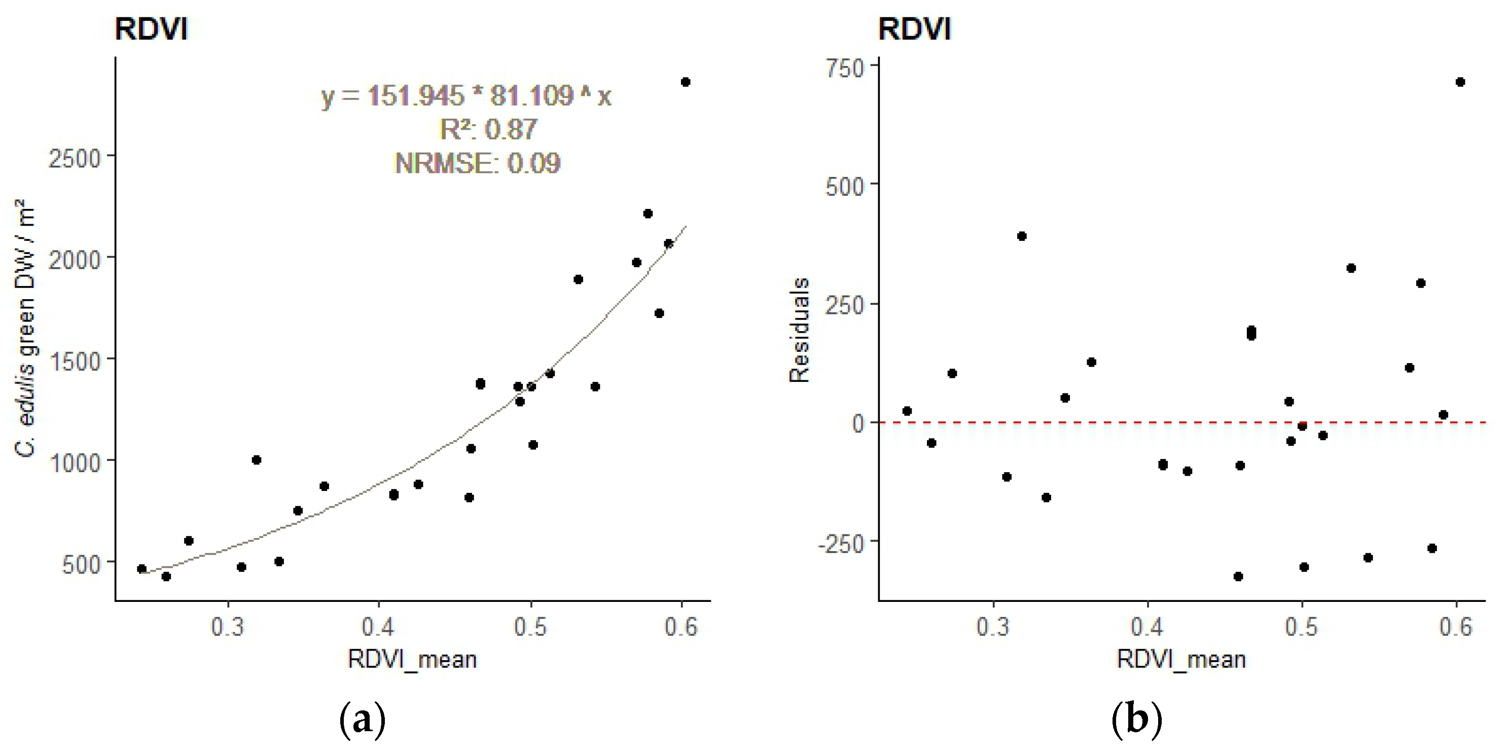
Figure A2.
– Regression model relating C. edulis DW to the best performing VI for the 5 cm GSD survey - sample points and regression line with equation (a), and residuals plot (b).
Figure A2.
– Regression model relating C. edulis DW to the best performing VI for the 5 cm GSD survey - sample points and regression line with equation (a), and residuals plot (b).
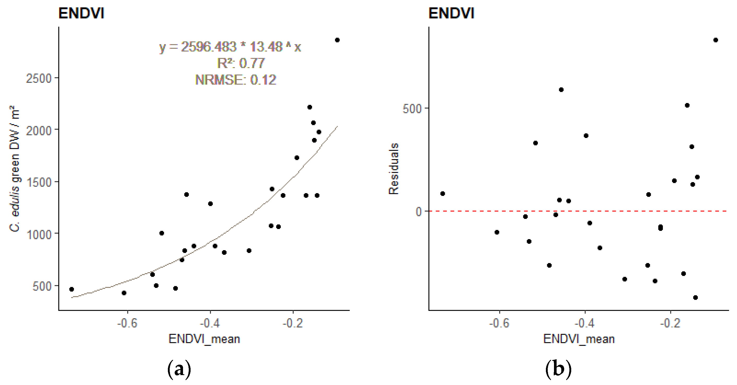
Figure A3.
– Regression model relating C. edulis DW to the best performing VI for the 10 cm GSD survey - sample points and regression line with equation (a), and residuals plot (b)..
Figure A3.
– Regression model relating C. edulis DW to the best performing VI for the 10 cm GSD survey - sample points and regression line with equation (a), and residuals plot (b)..
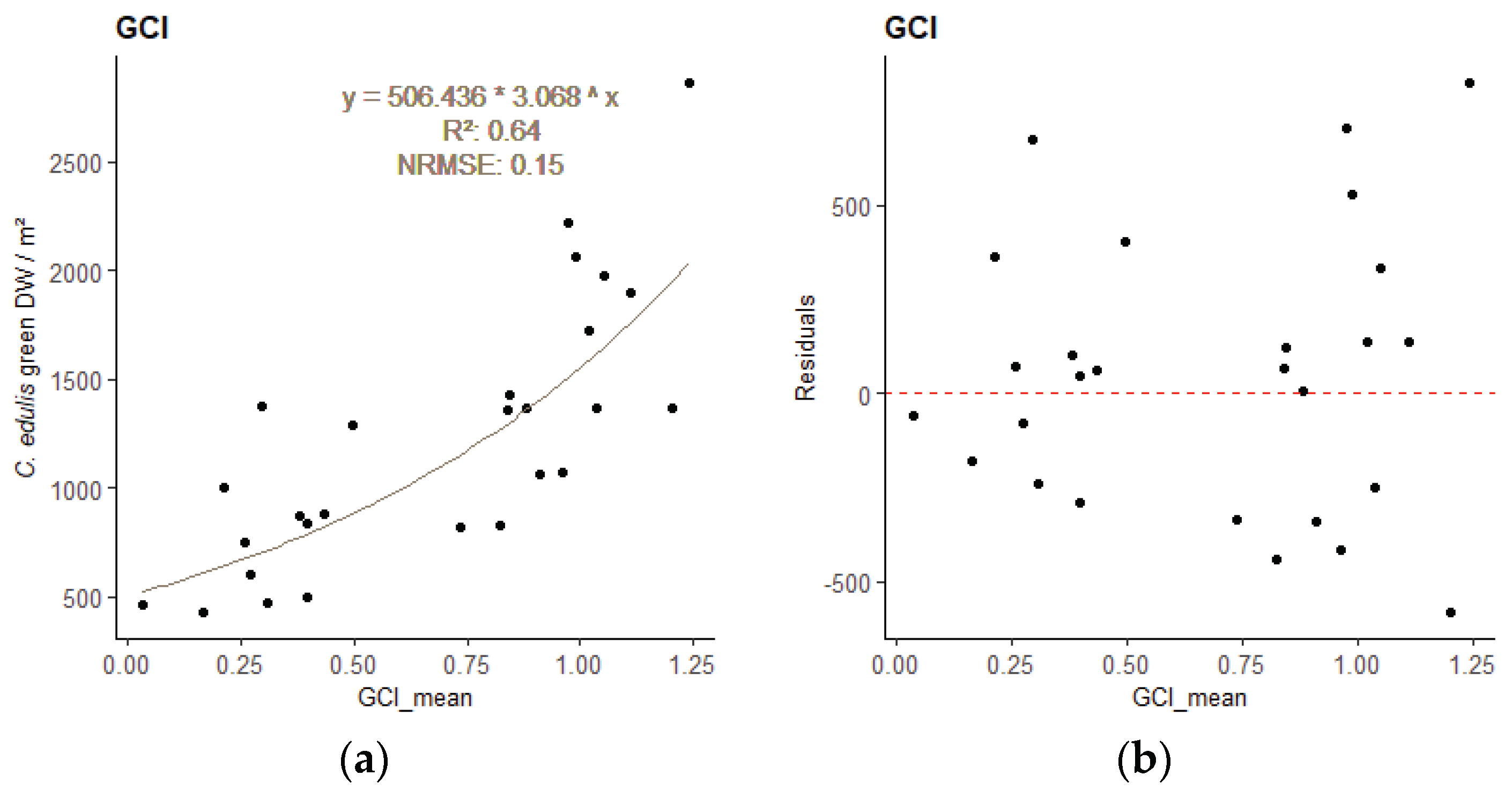
Table A4.
– Vegetation Indices empirical regression results, ordered by R². Best performing indices for each GSD resolution are marked in green.
Table A4.
– Vegetation Indices empirical regression results, ordered by R². Best performing indices for each GSD resolution are marked in green.
 |
References
- Tu, W.; Zhang, Y.; Li, Q.; Mai, K.; Cao, J. Scale Effect on Fusing Remote Sensing and Human Sensing to Portray Urban Functions. IEEE Geosci. Remote Sensing Lett. 2021, 18, 38–42. [CrossRef]
- Stückemann, K.-J.; Waske, B. Mapping Lower Saxony’s Salt Marshes Using Temporal Metrics of Multi-Sensor Satellite Data. International Journal of Applied Earth Observation and Geoinformation 2022, 115, 103123. [CrossRef]
- Doughty, C.L.; Ambrose, R.F.; Okin, G.S.; Cavanaugh, K.C. Characterizing Spatial Variability in Coastal Wetland Biomass across Multiple Scales Using UAV and Satellite Imagery. Remote Sens Ecol Conserv 2021, 7, 411–429. [CrossRef]
- Zhou, Z.; Yang, Y.; Chen, B. Estimating Spartina Alterniflora Fractional Vegetation Cover and Aboveground Biomass in a Coastal Wetland Using SPOT6 Satellite and UAV Data. Aquatic Botany 2018, 144, 38–45. [CrossRef]
- Guo, M.; Li, J.; Sheng, C.; Xu, J.; Wu, L. A Review of Wetland Remote Sensing. Sensors 2017, 17, 777. [CrossRef]
- Gonçalves, C.; Santana, P.; Brandão, T.; Guedes, M. Automatic Detection of Acacia Longifolia Invasive Species Based on UAV-Acquired Aerial Imagery. Information Processing in Agriculture 2022, 9, 276–287. [CrossRef]
- Mallmann, C.L.; Zaninni, A.F.; Filho, W.P. Vegetation Index Based In Unmanned Aerial Vehicle (Uav) To Improve The Management Of Invasive Plants In Protected Areas, Southern Brazil. In Proceedings of the 2020 IEEE Latin American GRSS & ISPRS Remote Sensing Conference (LAGIRS); IEEE: Santiago, Chile, March 2020; pp. 66–69.
- Abeysinghe, T.; Simic Milas, A.; Arend, K.; Hohman, B.; Reil, P.; Gregory, A.; Vázquez-Ortega, A. Mapping Invasive Phragmites Australis in the Old Woman Creek Estuary Using UAV Remote Sensing and Machine Learning Classifiers. Remote Sensing 2019, 11, 1380. [CrossRef]
- Huete, A.; Lyon, J.G.; Thenkabail, P.S. Hyperspectral Remote Sensing of Vegetation; Second Edition.; CRC Press: New York, NY, 2016; ISBN 978-1-4398-4538-7.
- Bian, C.; Shi, H.; Wu, S.; Zhang, K.; Wei, M.; Zhao, Y.; Sun, Y.; Zhuang, H.; Zhang, X.; Chen, S. Prediction of Field-Scale Wheat Yield Using Machine Learning Method and Multi-Spectral UAV Data. Remote Sensing 2022, 14, 1474. [CrossRef]
- Yang, S.; Hu, L.; Wu, H.; Ren, H.; Qiao, H.; Li, P.; Fan, W. Integration of Crop Growth Model and Random Forest for Winter Wheat Yield Estimation From UAV Hyperspectral Imagery. IEEE J. Sel. Top. Appl. Earth Observations Remote Sensing 2021, 14, 6253–6269. [CrossRef]
- Li, B.; Xu, X.; Zhang, L.; Han, J.; Bian, C.; Li, G.; Liu, J.; Jin, L. Above-Ground Biomass Estimation and Yield Prediction in Potato by Using UAV-Based RGB and Hyperspectral Imaging. ISPRS Journal of Photogrammetry and Remote Sensing 2020, 162, 161–172. [CrossRef]
- Santos, L.M.; Ferraz, G.A.S.; Diotto, A.V.; Barbosa, B.D.S.; Maciel, D.T.; Andrade, M.T.; Ferraz, P.F.P.; Rossi, G. Coffee Crop Coefficient Prediction as a Function of Biophysical Variables Identified from RGB UAS Images. 2020, 566.5Kb. [CrossRef]
- Wengert, M.; Wijesingha, J.; Schulze-Brüninghoff, D.; Wachendorf, M.; Astor, T. Multisite and Multitemporal Grassland Yield Estimation Using UAV-Borne Hyperspectral Data. Remote Sensing 2022, 14, 2068. [CrossRef]
- Wijesingha, J.; Astor, T.; Schulze-Brüninghoff, D.; Wachendorf, M. Mapping Invasive Lupinus Polyphyllus Lindl. in Semi-Natural Grasslands Using Object-Based Image Analysis of UAV-Borne Images. PFG 2020, 88, 391–406. [CrossRef]
- Brunel, S.; Brundu, G.; Fried, G. Eradication and Control of Invasive Alien Plants in the M Editerranean B Asin: Towards Better Coordination to Enhance Existing Initiatives. EPPO Bulletin 2013, 43, 290–308. [CrossRef]
- Gomes, P.T.; Botelho, A.A.; Soares de Carvalho, G. Sistemas dunares do litoral de Esposende; Universidade do Minho: Braga, 2002; ISBN 978-972-9027-16-1.
- Soares, C.; Granja, H.; P., G.; E., L.; Renato, H.; I., R.; L., C.; RIBEIRO New Data and New Ideas Concerning Recent Geomorphological Changes in the NW Coastal Zone of Portugal.; January 2002.
- Conser, C.; Connor, E.F. Assessing the Residual Effects of Carpobrotus Edulis Invasion, Implications for Restoration. Biol Invasions 2009, 11, 349–358. [CrossRef]
- Meyer, M.D.F.; Gonçalves, J.A.; Cunha, J.F.R.; Ramos, S.C.D.C.E.S.; Bio, A.M.F. Application of a Multispectral UAS to Assess the Cover and Biomass of the Invasive Dune Species Carpobrotus Edulis. Remote Sensing 2023, 15, 2411. [CrossRef]
- Gitelson, A.A. Remote Estimation of Canopy Chlorophyll Content in Crops. Geophys. Res. Lett. 2005, 32, L08403. [CrossRef]
- Richardson, A.D.; Duigan, S.P.; Berlyn, G.P. An Evaluation of Noninvasive Methods to Estimate Foliar Chlorophyll Content. New Phytologist 2002, 153, 185–194. [CrossRef]
- Tucker, C.J.; Elgin, J.H.; McMurtrey, J.E.; Fan, C.J. Monitoring Corn and Soybean Crop Development with Hand-Held Radiometer Spectral Data. Remote Sensing of Environment 1979, 8, 237–248. [CrossRef]
- Rasmussen, J.; Ntakos, G.; Nielsen, J.; Svensgaard, J.; Poulsen, R.N.; Christensen, S. Are Vegetation Indices Derived from Consumer-Grade Cameras Mounted on UAVs Sufficiently Reliable for Assessing Experimental Plots? European Journal of Agronomy 2016, 74, 75–92. [CrossRef]
- Gitelson, A.A.; Kaufman, Y.J.; Merzlyak, M.N. Use of a Green Channel in Remote Sensing of Global Vegetation from EOS-MODIS. Remote Sensing of Environment 1996, 58, 289–298. [CrossRef]
- Rouse, J.W.; Haas, R.H.; Deering, D.W.; Schell, J.A.; Harlan, J.C. Monitoring the Vernal Advancement and Retrogradation (Green Wave Effect) of Natural Vegetation. [Great Plains Corridor].; 1973.
- Gamon, J.A.; Peñuelas, J.; Field, C.B. A Narrow-Waveband Spectral Index That Tracks Diurnal Changes in Photosynthetic Efficiency. Remote Sensing of Environment 1992, 41, 35–44. [CrossRef]
- Roujean, J.-L.; Breon, F.-M. Estimating PAR Absorbed by Vegetation from Bidirectional Reflectance Measurements. Remote Sensing of Environment 1995, 51, 375–384. [CrossRef]
- Pearson, R.L.; Miller, L.D.; Program, U.S.I.B. Remote Mapping of Standing Crop Biomass for Estimation of the Productivity of the Shortgrass Prairie, Pawnee National Grasslands, Colorado; IBP Grassland Biome; Department of Watershed Sciences, College of Forestry and Natural Resources, Colorado State University, 1972;
- Olofsson, P.; Foody, G.M.; Herold, M.; Stehman, S.V.; Woodcock, C.E.; Wulder, M.A. Good Practices for Estimating Area and Assessing Accuracy of Land Change. Remote Sensing of Environment 2014, 148, 42–57. [CrossRef]
- Karasiak, N. Dzetsaka Qgis Classification Plugin 2016.
- Congedo, L. Semi-Automatic Classification Plugin: A Python Tool for the Download and Processing of Remote Sensing Images in QGIS. JOSS 2021, 6, 3172. [CrossRef]
- Papp, L.; van Leeuwen, B.; Szilassi, P.; Tobak, Z.; Szatmári, J.; Árvai, M.; Mészáros, J.; Pásztor, L. Monitoring Invasive Plant Species Using Hyperspectral Remote Sensing Data. Land 2021, 10, 29. [CrossRef]
- Sabat-Tomala, A.; Raczko, E.; Zagajewski, B. Comparison of Support Vector Machine and Random Forest Algorithms for Invasive and Expansive Species Classification Using Airborne Hyperspectral Data. Remote Sensing 2020, 12, 516. [CrossRef]
- Michez, A.; Piégay, H.; Jonathan, L.; Claessens, H.; Lejeune, P. Mapping of Riparian Invasive Species with Supervised Classification of Unmanned Aerial System (UAS) Imagery. International Journal of Applied Earth Observation and Geoinformation 2016, 44, 88–94. [CrossRef]
- Li, R.; Gao, X.; Shi, F.; Zhang, H. Scale Effect of Land Cover Classification from Multi-Resolution Satellite Remote Sensing Data. Sensors 2023, 23, 6136. [CrossRef]
- Guan, S.; Fukami, K.; Matsunaka, H.; Okami, M.; Tanaka, R.; Nakano, H.; Sakai, T.; Nakano, K.; Ohdan, H.; Takahashi, K. Assessing Correlation of High-Resolution NDVI with Fertilizer Application Level and Yield of Rice and Wheat Crops Using Small UAVs. Remote Sensing 2019, 11, 112. [CrossRef]
- Hassan, M.A.; Yang, M.; Rasheed, A.; Yang, G.; Reynolds, M.; Xia, X.; Xiao, Y.; He, Z. A Rapid Monitoring of NDVI across the Wheat Growth Cycle for Grain Yield Prediction Using a Multi-Spectral UAV Platform. Plant Science 2019, 282, 95–103. [CrossRef]
- Pandey, P.C.; Anand, A.; Srivastava, P.K. Spatial Distribution of Mangrove Forest Species and Biomass Assessment Using Field Inventory and Earth Observation Hyperspectral Data. Biodivers Conserv 2019, 28, 2143–2162. [CrossRef]
- Huang, S.; Tang, L.; Hupy, J.P.; Wang, Y.; Shao, G. A Commentary Review on the Use of Normalized Difference Vegetation Index (NDVI) in the Era of Popular Remote Sensing. J. For. Res. 2021, 32, 1–6. [CrossRef]
- Tenreiro, T.R.; García-Vila, M.; Gómez, J.A.; Jiménez-Berni, J.A.; Fereres, E. Using NDVI for the Assessment of Canopy Cover in Agricultural Crops within Modelling Research. Computers and Electronics in Agriculture 2021, 182, 106038. [CrossRef]
- Xu, Y.; Yang, Y.; Chen, X.; Liu, Y. Bibliometric Analysis of Global NDVI Research Trends from 1985 to 2021. Remote Sensing 2022, 14, 3967. [CrossRef]
- Innangi, M.; Marzialetti, F.; Di Febbraro, M.; Acosta, A.T.R.; De Simone, W.; Frate, L.; Finizio, M.; Villalobos Perna, P.; Carranza, M.L. Coastal Dune Invaders: Integrative Mapping of Carpobrotus Sp. Pl. (Aizoaceae) Using UAVs. Remote Sensing 2023, 15, 503. [CrossRef]
Figure 1.
Location of study area (red) in Iberian Peninsula (a); study area (b).
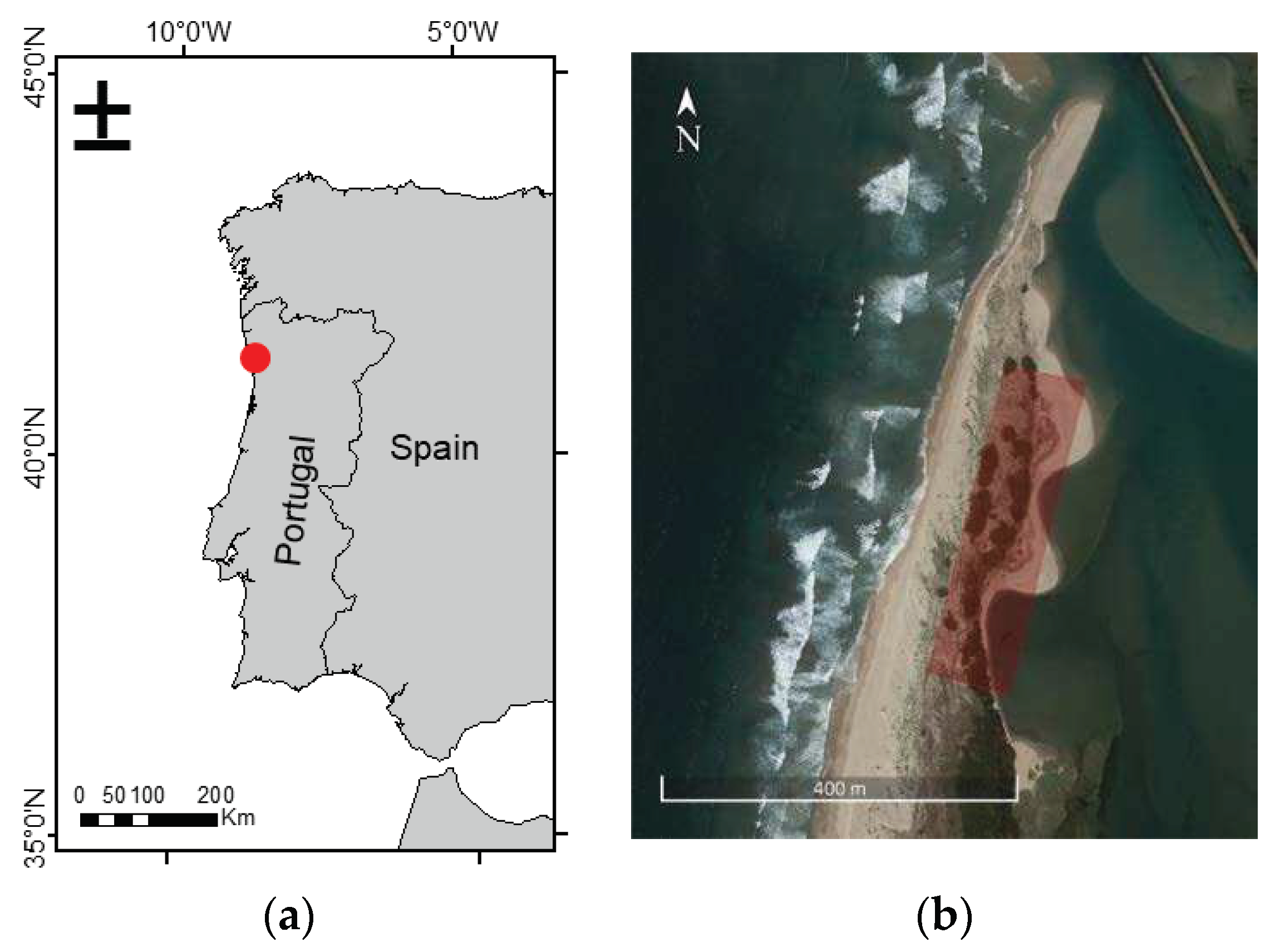
Figure 2.
placement of a quadrat on a C. edulis patch, with other vegetation covers visible to the left (various herbaceous species) and in the back (acacia) (a); delimitation of the central 30 × 30 cm2 area within a quadrat for AGB removal (b); brown layer of C. edulis after removal of the top green layer (c).
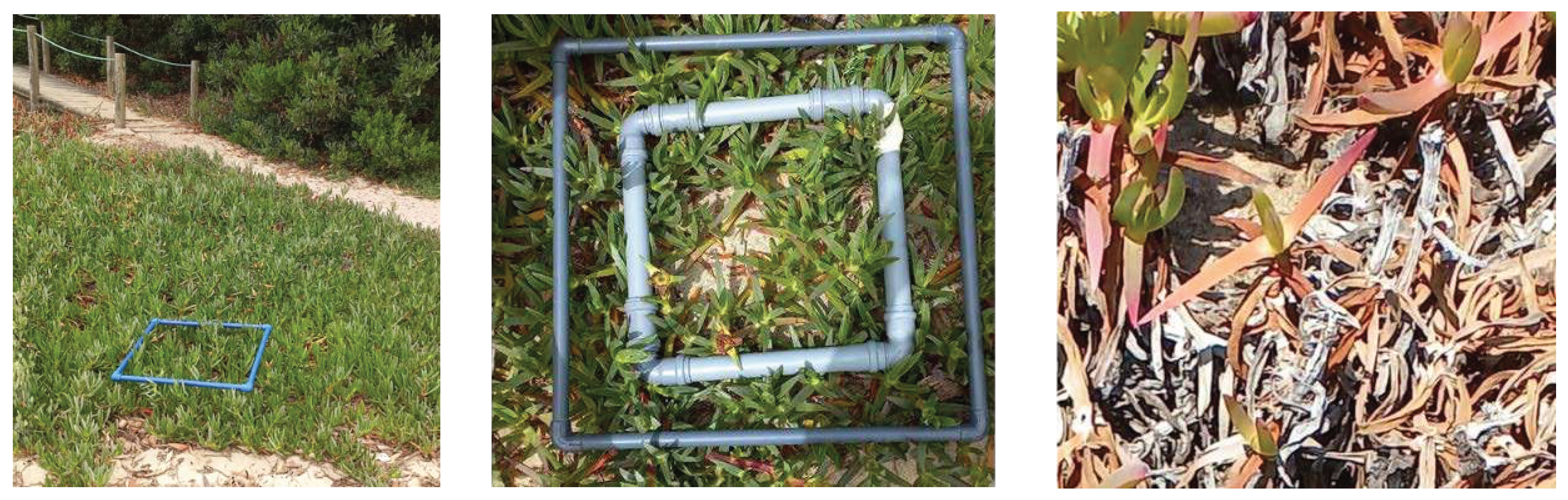
Figure 5.
Representative area of the Land Cover Classification for each of the resolutions.
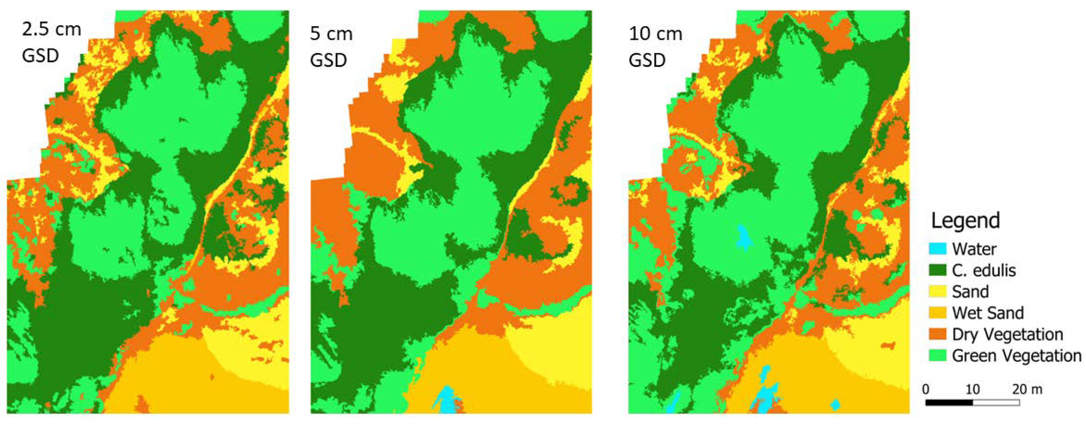
Figure 9.
Orthomosaic cover changes comparison between resolutions, for the areas classified as C. edulis using the 2.5cm GSD imagery.
Figure 9.
Orthomosaic cover changes comparison between resolutions, for the areas classified as C. edulis using the 2.5cm GSD imagery.
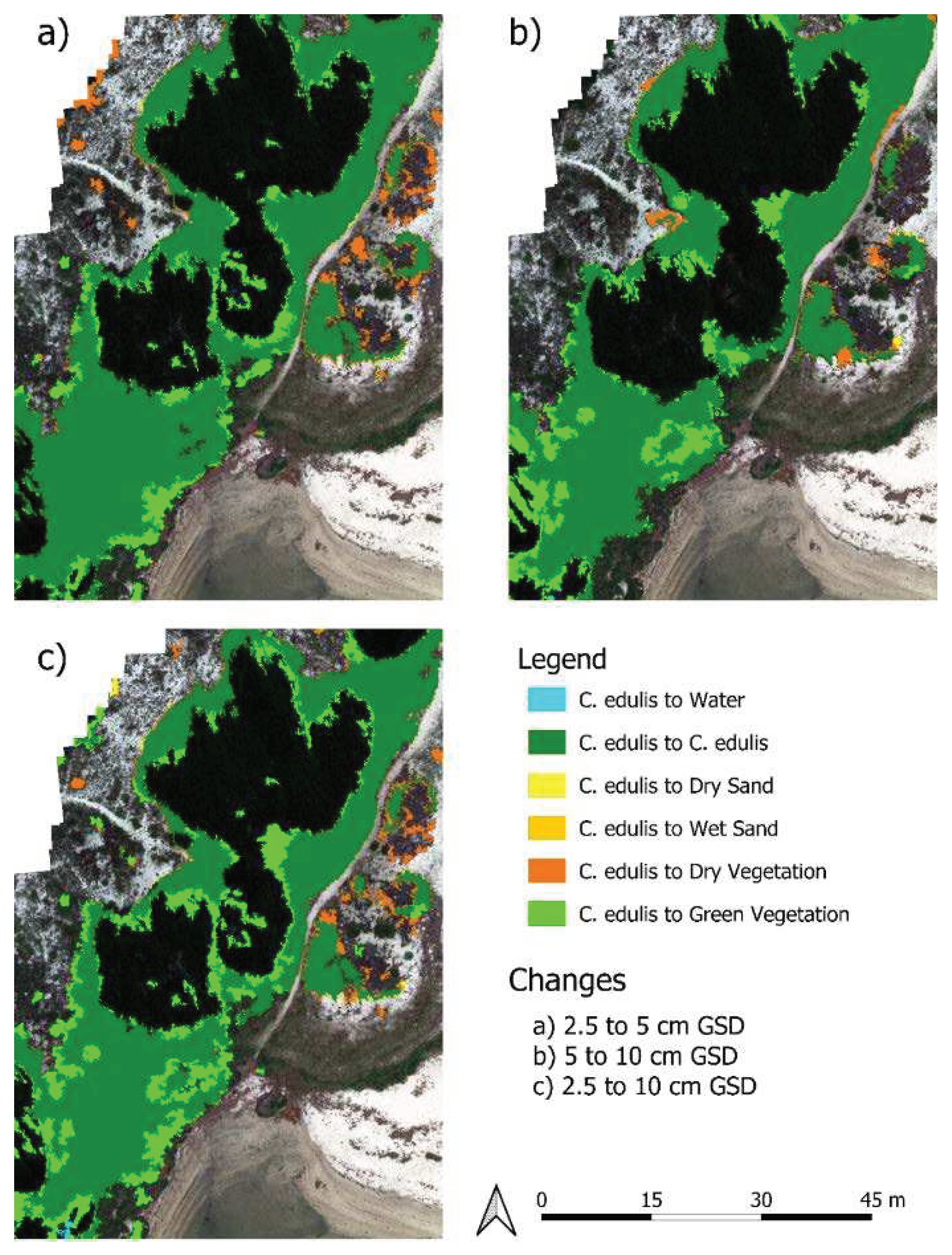
Table 1.
Vegetation indices formulas used in this work. Bands: Blu—Blue; Gre—Green; RDG—Red Edge; NIR—Near Infrared.
Table 1.
Vegetation indices formulas used in this work. Bands: Blu—Blue; Gre—Green; RDG—Red Edge; NIR—Near Infrared.
| Index | Formula | Reference |
|---|---|---|
| Green Chlorophyll Index (GCI) | [21] | |
| Difference Vegetation Index (DVI) | [22] | |
| Green Difference Vegetation Index (GDVI) | [23] | |
| Enhanced Normalized Difference Vegetation Index (ENDVI) | [24] | |
| Green Normalized Difference Vegetation Index (GNDVI) | [25] | |
| Normalized Difference Vegetation Index (NDVI) | [26] | |
| Photochemical Reflectance Index (PRI) | [27] | |
| Renormalized Difference Vegetation Index (RDVI) | [28] | |
| Ratio Vegetation Index (RVI) | [29] |
Table 3.
Summary statistics of C. edulis sample wet weights (WW) and dry weights (DW) for the plants’ green and brown parts (SD: standard deviation).
Table 3.
Summary statistics of C. edulis sample wet weights (WW) and dry weights (DW) for the plants’ green and brown parts (SD: standard deviation).
| GREEN | BROWN | |||
| WW (kg/m²) | DW (kg/m²) | WW (kg/m²) | DW (kg/m²) | |
| Highest | 27.12 | 2.86 | 3.65 | 2.64 |
| Lowest | 2.09 | 4.66 | 0 | 0 |
| Mean | 9.68 | 1.27 | 1.01 | 0.62 |
| Median | 8.16 | 1.07 | 0.51 | 0.29 |
| SD | 6.43 | 0.71 | 1.13 | 0.73 |
Table 4.
Best DWgeen – VI regression model for each resolution with respective R², RMSE, NRMSE, model and respective coefficients a and b.
Table 4.
Best DWgeen – VI regression model for each resolution with respective R², RMSE, NRMSE, model and respective coefficients a and b.
| GSD (cm) | Index | R² | RMSE | NRMSE | Model | Coef a | Coef b |
|---|---|---|---|---|---|---|---|
| 2.5 | RDVI | 0.87 | 227.18 | 0.09 | 151.94 | 81.11 | |
| 5 | ENDVI | 0.77 | 300.67 | 0.12 | 2596.48 | 13.48 | |
| 10 | GCI | 0.64 | 364.55 | 0.15 | 506.44 | 3.07 |
Disclaimer/Publisher’s Note: The statements, opinions and data contained in all publications are solely those of the individual author(s) and contributor(s) and not of MDPI and/or the editor(s). MDPI and/or the editor(s) disclaim responsibility for any injury to people or property resulting from any ideas, methods, instructions or products referred to in the content. |
© 2024 by the authors. Licensee MDPI, Basel, Switzerland. This article is an open access article distributed under the terms and conditions of the Creative Commons Attribution (CC BY) license (http://creativecommons.org/licenses/by/4.0/).
Copyright: This open access article is published under a Creative Commons CC BY 4.0 license, which permit the free download, distribution, and reuse, provided that the author and preprint are cited in any reuse.


