Preprint
Article

This version is not peer-reviewed.

Estimating Biomass and Above-Ground Carbon in Wetlands: Influence of Plot Size and Sample Data Treatment in a Model Based on Remote Sensing and Random Forest

A peer-reviewed article of this preprint also exists.

Submitted:

21 February 2025

Posted:

24 February 2025

You are already at the latest version

Abstract

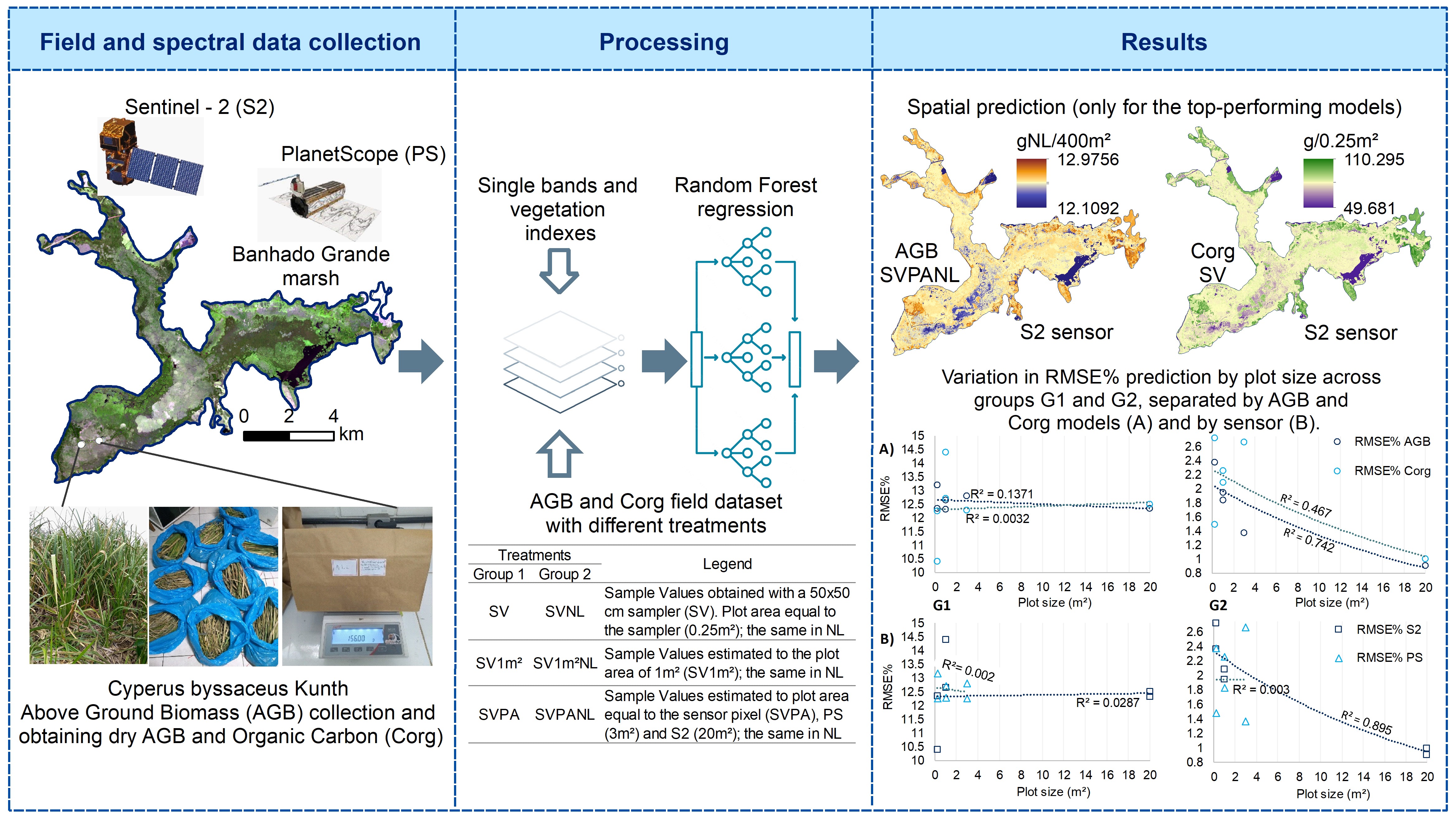
Wetlands are essential carbon sinks in the global ecosystem, absorbing CO2 in their biomass and soils and mitigating global warming. Accurate above-ground biomass (AGB) and organic carbon (Corg) estimation is crucial for wetland carbon sink research. Remote sensing (RS) data effectively estimates and maps AGB and Corg in wetlands using various techniques, but there is still room to improve the efficiency of Machine Learning (ML) based approaches. This study examined how different sample data treatments and plot sizes impact a Random Forest model’s performance based on RS for AGB and Corg prediction. The model was trained with samples of emergent vegetation collected in a palustrine wetland in southern Brazil and spectral variables (single bands and Vegetation Indices — VI) from medium and high-resolution optical images, Sentinel 2 and PlanetScope, respectively. The treatments involve the AGB and Corg values dimensioned for three different plot sizes (Group 1) and the same subjected to the Natural Logarithmic normalization — NL (Group 2). Therefore, six AGB and Corg models were created for each sensor. Models and sensor performances and spectral variable importance were compared. In our results, NL-normalized sample data RF models proved more accurate. Larger plots produced smaller prediction errors with S2 models, indicating the influence of plot size on the reliability of the estimate. S2 surpassed PS in AGB/Corg prediction, but PS was superior in mapping spatial variability. The VI CO2Flux and S2’s SWIR, Blue, Green, and RE bands 6 and 7, were more importance for AGB/Corg prediction. The innovation of this study is that, in addition to optimizing RF model parameters, optimizing the AGB and Corg dataset collected in the field, i.e., evaluating normalization and plot sizes, is crucial to obtain more accurate estimates with RS and ML-based models. This approach, integrated with Sentinel 2’s medium-resolution data and the combination of VIs and bands, enhances AGB/Corg stock estimation and monitoring in wetlands, and the highlighted predictors can act as spectral indicators of these ecological functions.

Keywords: 
;  ;  ;  ;  

1. Introduction

Due to the unique biogeochemical processes of wetland ecosystems, their structure, and location, they possess valuable ecological functions that provide ecosystem services to human populations [1,2,3], with high economic values [4]. Wetlands act as significant carbon reservoirs and play an important process in the global carbon cycle [5]. The above-ground biomass of wetland vegetation (AGB) is a critical indicator of the capacity for carbon dioxide assimilation and organic carbon (Corg) storage [5,6]. Research on carbon storage in wetland vegetation and the precise spatial estimation of AGB and Corg are important for studying their influence on the global carbon cycle, especially in relation to climate change [6,7] and meeting the main global goals of reducing greenhouse gas (GHG) emissions.
Data obtained through remote sensing (RS) are utilized to characterize, estimate, and monitor these ecosystem functions of wetlands [8,9]. They provide biophysical indicators [10] linked to the ecological processes of vegetation, such as photosynthesis, primary productivity, biomass, and carbon fluxes, drivers for various functions [11]. As biophysical indicators, spectral indices such as the Normalized Difference Vegetation Index (NDVI) and the Enhanced Vegetation Index (EVI), among others, are conceptually linked to the aforementioned vegetative processes [12].
Predictive models for AGB and Corg based on RS employ in situ data or allometric equations to “train” algorithms and create rules from satellite imagery, including physical, statistical, and Machine Learning (ML) approaches. Statistical methods such as simple and multiple Linear Regression (LR) are practical to compute; however, they must meet basic assumptions like data normality and variance homogeneity, among others. The results are satisfactory with few field samples and various spectral variables, which makes them quite popular [13,14,15]. Nonetheless, they do not effectively describe the complex non-linear relationship between AGB, Corg, and RS data [16].
ML methods such as Random Forest Regression (RF), decision tree-based (DT), K-Nearest Neighbors (KNN), Artificial Neural Network (ANN), and Support Vector Machine (SVM) enhance the non-linear estimates of AGB and Corg in wetlands from RS data. Algorithms like RF and Gradient Boosting perform excellently in modeling these variables [7,16,17].
One of the advantages of ML methods such as RF is that it is not necessary to formulate hypotheses regarding data distribution or assumptions that need to be met [18]. Being a distribution-free method, it allows the integration of data from different sources without transformations or normalization and achieves an excellent relationship with the target variable [18,19]. Previous research utilized linear and ML models and applied Normalized Logarithmic transformation only to the linear models [20,21] while others applied them to both models [22,23]. The influence of data normalization on the performance of RF and others ML models has been empirically studied in datasets from the business, health, and agriculture [24], showing that data normalization contributes to more accurate modeling. However, its influence on the performance of RF and RS-based models in estimating of AGB and Corg remains unexplored to date.
Regardless of the employed model, errors, and uncertainties in predicting AGB and Corg in wetlands can arise from various sources, primarily including sample design and field data collection methods, such as sample size variation [13], plot size [22,25], collection frequency [26], differences between field sampling scales and satellite images, the timing of field data and image acquisition, and image data extraction protocols [27].
The treatment of field-collected data and its use in models also varies. Some directly use the AGB value collected at each point [27,28]; sample data expressed in different area units [14,15]; the sample value estimated to the plot area [22]; the average of values collected in N plots [29,30]. The influence of sample plot size on the accuracy of AGB and Corg estimation models has been well explored in ecosystems with dense vegetation, such as forests and mangroves [22,31,32,33]. These studies demonstrate that larger plots contribute to more accurate predictions. However, similar studies in wetlands are rare and non-existent in herbaceous marshes. The absence of research on optimal plot size for remote monitoring and predictive models in wetlands impacts the consistency of predictions with the alike vegetation. Therefore, this study jointly examines the research gaps on the influence of different input data treatments and plot sizes on the accuracy of remote AGB and Corg estimation in wetlands using a ML model. This research aims to enhance remote estimation methods for AGB and Corg, expanding their application to wetland ecosystems, especially herbaceous wetlands.
Therefore, this study aims to answer (a) whether different sampling treatments and plot sizes affect the performance of a predictive model of AGB and Corg based on remote sensing and ML and the importance of the spectral variables used; (b) which sensors and spectral variables obtained, respectively, the most accurate estimate and the greatest predictive importance. We aim to explore these research gaps, with a special interest in improving RF models for the prediction and spatialization of AGB and Corg in wetlands. To this end, we utilized data from Sentinel 2A and PlanetScope sensors and field-collected data in a palustrine wetland in southern Brazil. The results, although based on species-specific models, provide a foundation for enhancing predictive ML models in wetlands. They offer crucial insights for AGB and Corg prediction models, with the potential to drive standardization in the collection and processing of input data for predictive models with the aim of ensuring consistent predictions in inventories and monitoring. In addition, it contributes to the understanding of these ecological processes in wetlands, especially in light of the difficulties of access and collections.

2. Data and Methods

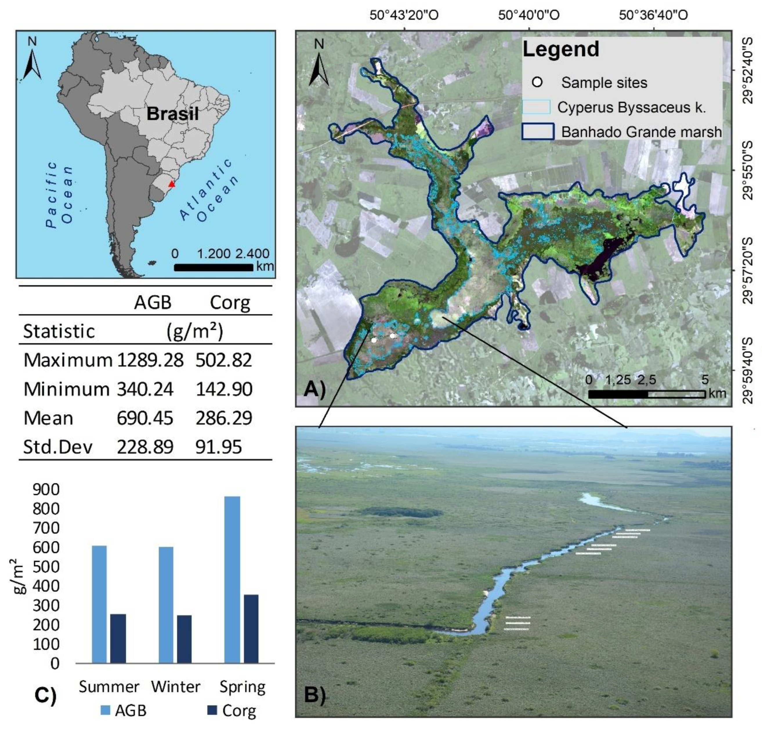
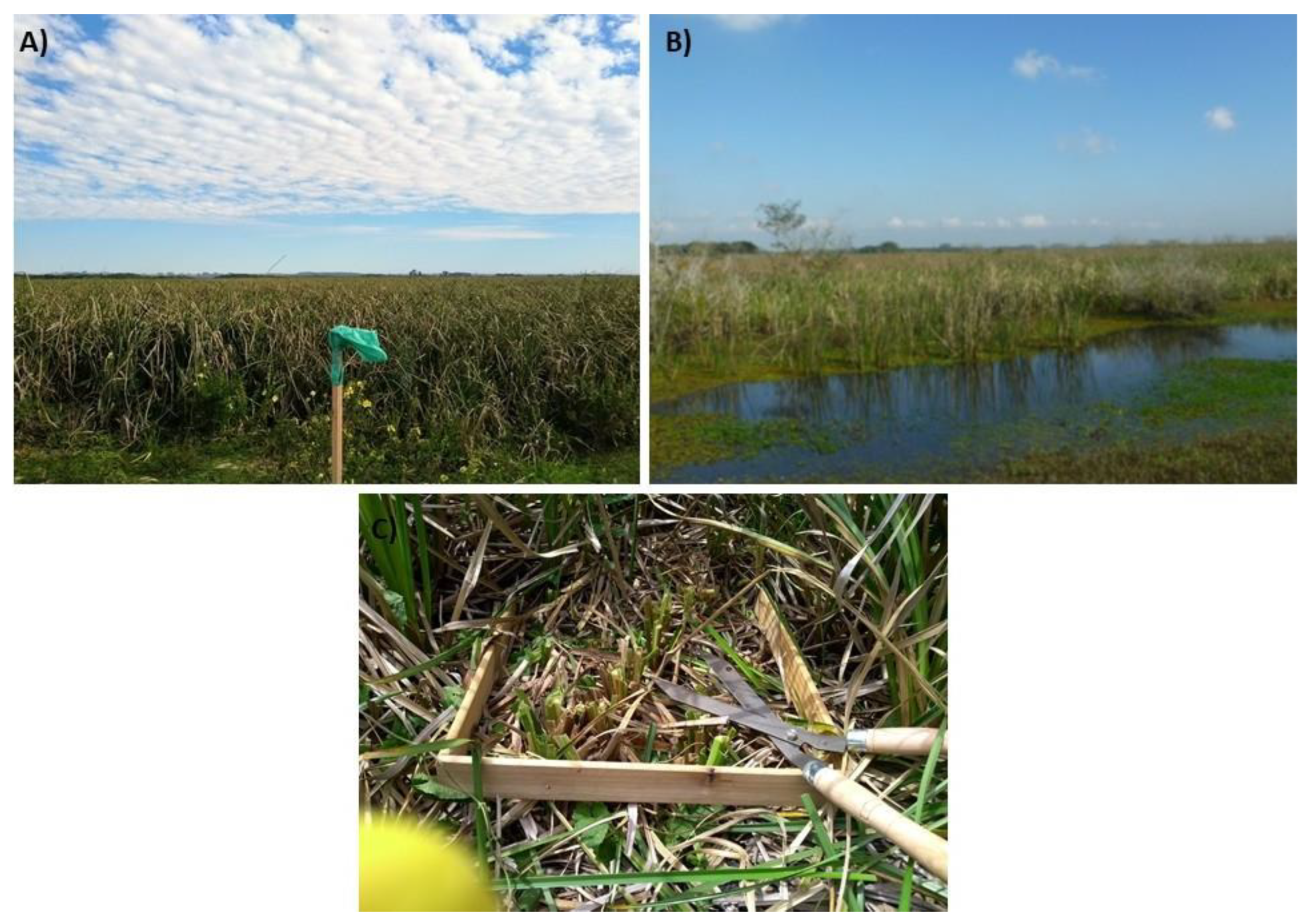
2.1. Study Area and Field Data Collection

Banhado Grande (BG) was used as a case study (29°57'S – 50°41'W, 5,591 ha) in the east of the state of Rio Grande do Sul (RS), in the geomorphological region of the Inner Coastal Plain, in a flat area with altimetry of up to 20 m (Figure 1). BG forms the Gravataí River and acts as a natural flow regulator, it is a palustrine environment integrated with the Banhado Grande Environmental Protection Area (EPABG) for sustainable use, comprising marsh areas, flood plains, and rice fields that become connected in periods of large flooding pulses [34].
The lithology is predominantly sedimentary environments of heterogeneous active peats, interconnected by floodplain deposits, interconnected by floodplain deposits composed of silt-clay sand [35,36]. The study area is located in a subtropical humid climate zone, with no defined rainy season [37].
The vegetation cover is dominated by macrophytes with heterogeneous distribution patterns, comprising the emerging species Scirpus giganteus, recently appointed as Cyperus byssaceus Kunth [38] with the most representative area and coverage in monodominance in the marsh, extending for ∼1,507 ha [39], represented by the light blue polygon (Figure 1A) and it occurs in areas with a presence of active peat bogs [40].
The species is caespitose perennial, between 80-170 cm tall, is widely distributed in the south of South America, in freshwater and silted marshes and along the banks of creeks and small streams, with an emergent and amphibious biological form [38,41,42], (Figure 2A and 2B). The flooding regime in the area where Cyperus byssaceus occurs is intermittent or only saturated soils [34].
The summarized methodological flow is described in the Graphical Abstract of the research, and further details are provided in this section. The field campaign was carried out throughout one annual cycle in 2018, at the end of the summer, winter, and spring (Table 1), periods characterized by low rainfall. The sampling survey was designed so that each plot corresponded to a transect similar to a 20m × 20m Sentinel pixel. Nine plots were fixed with stakes, spaced at least 40m apart (Figure 1B). The center position of the plots was recorded using Global Positioning System (GPS) equipment, Etrex Legend model, with a margin of error of 3m. The plots were positioned in an extensive area with a monospecific predominance of Cyperus byssaceus so that the collection of reflectance data in the images would not occur outside the areas with the desired plants, due to possible positioning errors by the GPS and the sensors.
In each plot, three samples were collected at random, totaling 27 AGB samples, according to the sampling guidelines [43,44]. A 50 cm × 50 cm square (0.25 m²) was used to collect the vegetation on the soil surface (Figure 2C). The samples were packed and dried in an oven at 60 °C until they reached a constant weight. The dried AGB was then measured on a precision scale to obtain the dry weight expressed in grams.
The Corg concentration was obtained using the Walkley Black wet combustion method, which returns the organic carbon content (%) in 100 g of dry weight of AGB, converted to Corg stocks based on direct proportion [44,45]. In general, the average AGB and Corg was 690 g/m² and 286 g/m², with the highest values observed in spring (Figure 1C) when new leaves are seen in greater quantity. During the campaign of field, no preferential periods of senescence were observed.

2.2. Remote Sensing Datasets

The Sentinel-2A images were obtained from the Sentinel Scientific Data Hub (ESA) in the 13 bands of the multispectral instrument (MSI) sensor. The visible (Blue, Green, and Red) and near-infrared (NIR) bands have a spatial resolution of 10 m; the Red Edge (RE5, RE6, RE7, and RE8A) and shortwave infrared (SWIR1 and SWIR2) bands have a spatial resolution of 20 m. Band 1 (coastal aerosol), Band 9 (water vapor), and Band 10 (cirrus) were excluded and not considered in this research.
The product is already orthorectified, georeferenced, and radiometrically calibrated into top-of-atmosphere (ToA) reflectance data, with pre-processing level 1C. The images were pre-processed to level 2A to remove atmospheric effects and convert pixel values to surface reflectance using Sen2Cor standalone tool [46], but can be processed alternatively in the S2A Toolbox of the Sentinel Application Platform (SNAP). The bands with resolutions of 10 m were downscaled to 20 m to ensure that all channels were concatenated with aligned pixels, using the nearest neighbor method, in the SNAP geometric operation tool.
Sentinel-2A and PlanetScope data were obtained as close as possible to the vegetation collection dates (Table 1).
Among the PlanetScope satellite constellation, we used data from the Planetscope-0, sometimes called Dove data, which detects the Blue, Green, Red, and NIR spectral bands. The Ortho Scene PlanetScope product was made available to the research team through the Planet Research and Education Program on the Planet Explorer website, with atmospherically corrected Level 3B surface reflectance and 3 m spatial resolution. The Ortho Scene product is distributed in images with radiance values (Planet Analytic product) and reflectance values (Planet Surface Reflectance-SR).
The SR product is derived from the Planet Analytic product, and the bands are co-acquired, orthorectified and georeferenced, with radiometric calibration in surface reflectance derived using the 6S radiative transfer code, assuming a continental aerosol model and using the closest available MODIS aerosol optical depth spatially and temporally, which guarantees consistency in all climatic conditions, minimizing the uncertainty of the spectral response in time and location [47].
In addition to the single-band information, we derived Vegetation indices (VIs) based on the band mathematics of the sensors’ reflectance images. The VIs were computed as indicated in Table 2.
These IVs were chosen because they are conceptually linked to the aforementioned vegetative processes and considered effective in characterizing and predicting AGB and Corg [12,51]. IVs Among the VIs, NDVI is often used successfully to estimate vegetation biomass in Wetlands [7,54] and in studies related to photosynthesis, carbon stocks and other plant-related processes [55]. Moreover, we use specific VIs adapted for wetlands, which are versions of the NDVI and EVI, such as the Normalized Difference Aquatic Vegetation Index (NDAVI) and the Water Adjusted Vegetation Index (WAVI).
To estimate Corg, the indices of Photochemical Reflectance (sPRI) and Integrated index (CO2Flux) are sensitive to changes in carotenoid pigments in leaves, indicative of the efficiency of the use of photosynthetic light related to the level of carbon dioxide stored by vegetation and vigor vegetation [56]. CO²flux is an integrated index, formed by the sPRI and NDVI VIs. A modified CO²flux index, replacing the traditional NDVI with NDVI adapted for wetlands (NDAVI) was also used. The spectral values of the bands and VIs were obtained from the pixels corresponding to the points of each sample site on Banhado Grande, from automatic extraction.

2.3. Development of the Prediction Models

A RF machine learning algorithm was used as the regression approach for this study. The RF is an efficient bagging-based ensemble learning method developed for improving the regression and classification tree by combining multiple decision trees [57].
The RF regression was implemented through Scikit-learn packages [58] in Python 3. The input sets were the single-bands and VIs of each sensor and the AGB and Corg samples separated as follows: the samples collected at each point with a 0.25m² sampler were proportionally estimated for plots of varying sizes (Group 1, Table 3). These were subjected to the Normalized Natural Logarithmic transformation— NL statistical treatment (Group 2, Table 3). The plot sizes were defined based on the most commonly used sizes in studies estimating biomass and above-ground carbon in wetlands using remote sensing. These sizes include: sampler size, sensor pixel size, or resized size, and this was determined following an extensive literature review."
In this manner, we generated six AGB and Corg models per sensor to compare accuracy in relation to treatments and plot sizes. Due to the characteristics of whole AGB and Corg values, the NL transformation is applied to strengthen the relationship with spectral data [13,59]. For each decision tree in RF, we utilized the bootstrapping method (random sampling with replacement) to select the original dataset. At each bootstrap resampling step, 2/3 of the data (in-bag) were selected to build the decision tree without pruning. The other 1/3 of the data (out-of-bag — OOB) were used as evaluation data and to calculate the OOB error as an unbiased estimate of prediction error [60].
The RF estimates the importance of predictors by calculating the total reduction in impurity (heterogeneity) brought about by these predictors. It is also known as the Gini importance. These variable importance values are then used to rank the predictors in terms of the strength of their relationship with the dependent variables (Breiman, 2001; Pedregosa et al., 2011) of AGB and Corg.
Finding the best combination of parameters is critical to the optimization of the model. To find the number of trees (Ntree) that best predicts AGB and Corg in each model, the Ntree parameter was optimized based on lower RMSE [18,28]. The test with the lowest RMSE and the lowest number of trees provides the optimal number of decision trees in the RF for a good compromise between accuracy and computational time [61]. The Ntree values were tested from 50 to 1000 with an interval of 50, while the number of predictor variables (bands and IVs) tested at each node (Mtry) and the standard node size were accepted throughout the analysis, which allows the regression trees to grow to their maximum size without pruning, based on the selection of predictor vectors that reduce the impurity of each node. The final regression model is based on the average value of all the results from the individual trees.

2.4. Evaluation of Models

The performance of the models was assessed using the best value of the R² parameters to assess the reliability of AGB predictions modelled by remote sensing [62], and Root Mean Square Error for in bag dates (RMSE) and % RMSE (relative), defined as the RMSE divided by the mean values of the field observations in the treatment. Typically, a higher R² score and a lower RMSE% value signify a model's ability to estimate information more accurately.
We also use the OOB data to generate predictions and to carry out an internal cross-validation technique for estimating of model prediction error by calculating the OOB Error [28,60,63]. The predictions from the OOB samples were used to compute RMSEOOB and RMSE%OOB.
The OOB estimate of error is considered to be a reliable assessment of predictive accuracy since the OOB data did not form part of the bootstrapped data sample as the inputs to the model [28,60]. Researches highlights that it is not necessary to have an independent validating dataset [57,64], and this is of particular interest regarding wetland areas, since data collection is difficult due to areas poor accessibility [28]. In the final stage of the study, the AGB and Corg maps were generated for the study area using the Rasterio Python library in Python 3.

3. Results

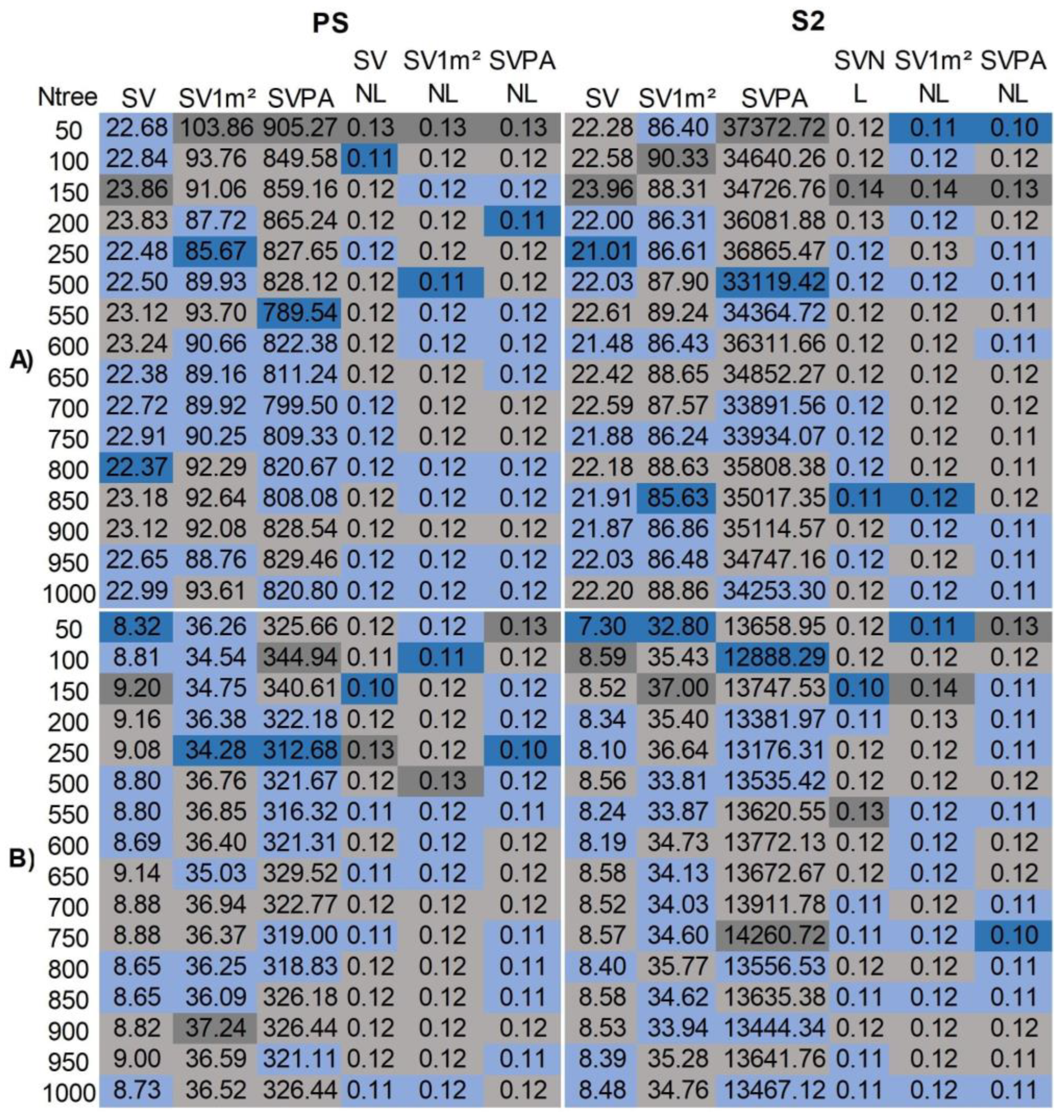
3.1. Optimization of Regression Model Parameters

RF algorithm was run repeatedly to obtain the optimum Ntree values. To optimize bagging trees, we varied the number of trees (Ntree) in the ensemble by adding 50 trees at a time and then recorded the resulting RMSE up to a maximum of 1000 trees. The optimal Ntree that produced the lowest RMSE in each model is highlighted in dark blue and the highest RMSEs in dark gray (Figure 3).
In general, the best accuracies occurred between low and medium Ntree values (up to 550) with PS sensor data and up to 850 with the S2 sensor. The results indicated that changes in Ntree parameters result in changes in RMSE, especially for models with treatments that are not normalized. It also indicates that exceeding the optimal Ntree does not improve the model's accuracy. Therefore, we selected the Ntree value with the lowest RMSE in each model to run the optimized regressions and will be presented these results in the next section.

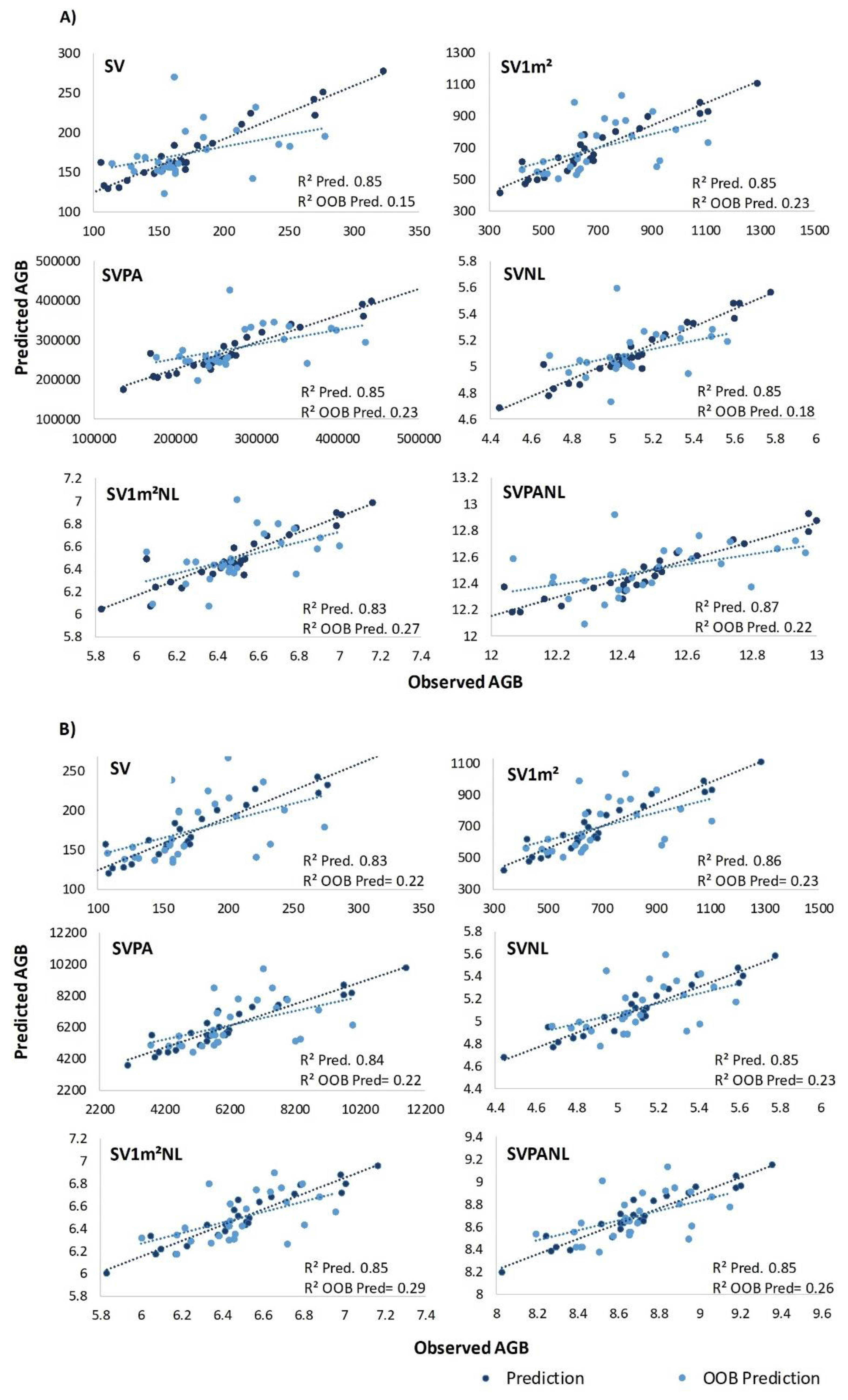
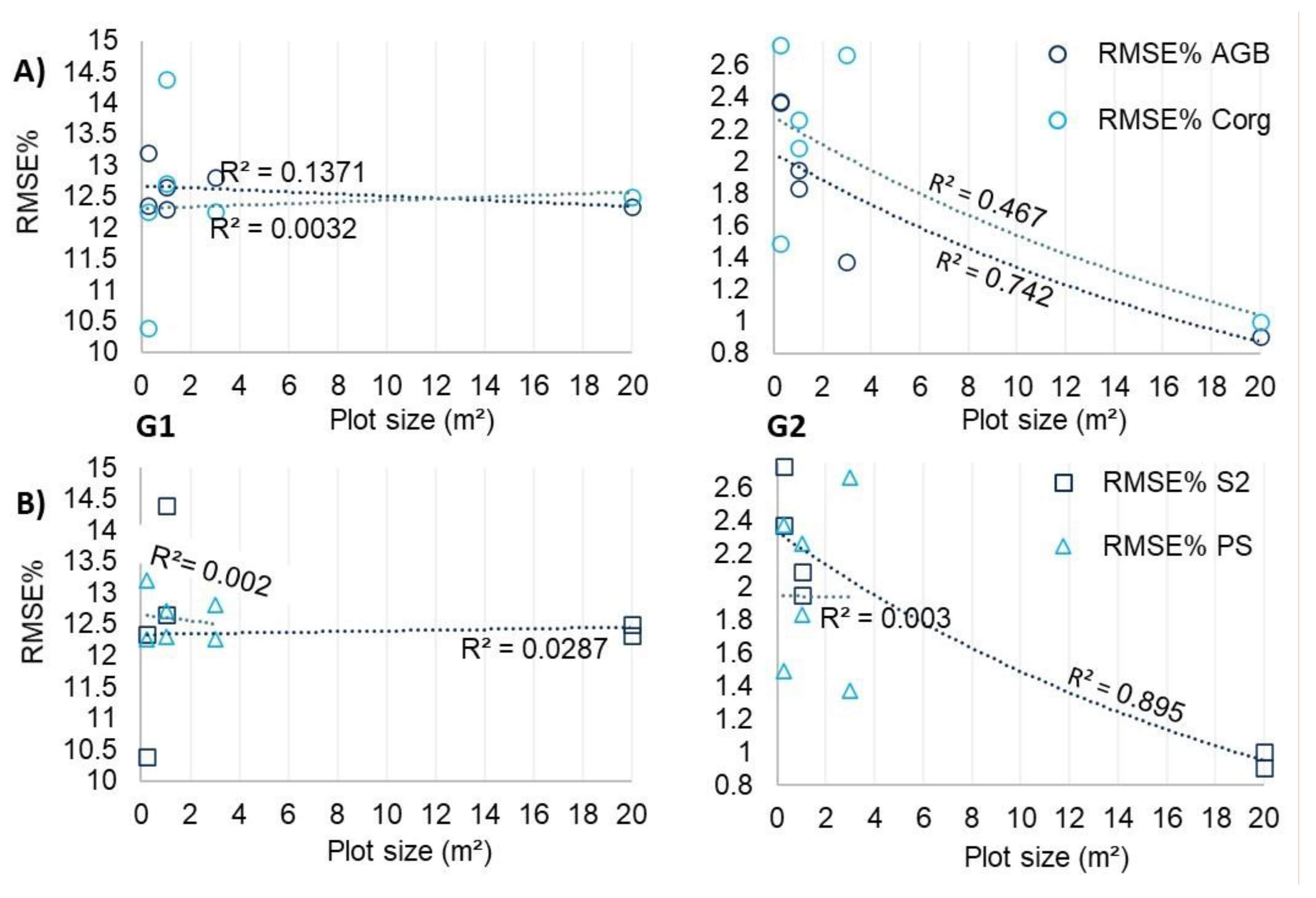
3.2. Predictive Performance of the RF Models

The performance of models could be explained by the Table 4 and by the scatterplots (Figure 4), which show the relationship between the observed AGB values and predicted AGB values in bag and OOB. The predictive performance of the models was assessed based on the lowest %RMSE OOB and %RMSE, in that order, and the highest R² between sensors and treatments in the same group. The model with the best AGB and Corg prediction performance was highlighted in bold in Table 4.
The best model among the sensors was that of S2 using treatments SVPANL for AGB (R² 0.87) and SV for Corg (R² 0.89). Their higher R² values better explained the variability of observed AGB and Corg, and %RMSE and %RMSE OOB showed less relative dispersion of predicted values in relation to observed values, compared to the best PS sensor models.
The treatment that was repeated the most with the best fit (3x) in group 2 and among all the models were SVPANL. In group 1 there was no predominance of the best performing treatment, but the model with SV treatment was repeated 2x and achieved the best R² (0.89) of all the models. In general, the models with treatments estimated to sensor Pixel Area prevailed with the best fits in predicting AGB and the models with treatments Sample Values prevailed with the best fits in predicting Corg para o sensor S2. No treatment prevailed between groups with the PS datasets, but SV1m² had the highest R² of 0.86.
Although the models achieved a good fit, they had moderate to low predictive accuracy when using the OOB dataset, with %RMSEOOB around 1x higher compared to the training dataset. All the models showed a tendency to overestimate, which can be seen when comparing the mean values observed versus predicted (Table 5). Note that even with a low R², the average AGB and Corg predicted with OOB data were very close to the average observed and training values.
We found a good fit between models performance and plot area variations under G2 treatments (Figure 5A), with distinct sensor relationships (Figure 5B). The AGB and Corg model errors (RMSE%) with G2 treatments show an exponential decay as plot size increases. Conversely, the models with G1 treatments and with PS sensor data do not explain the effect of plot size variation on model performance, indicated by low R² values. Unlike, the S2 models with G2 treatments were substantially better (R² = 0.89).

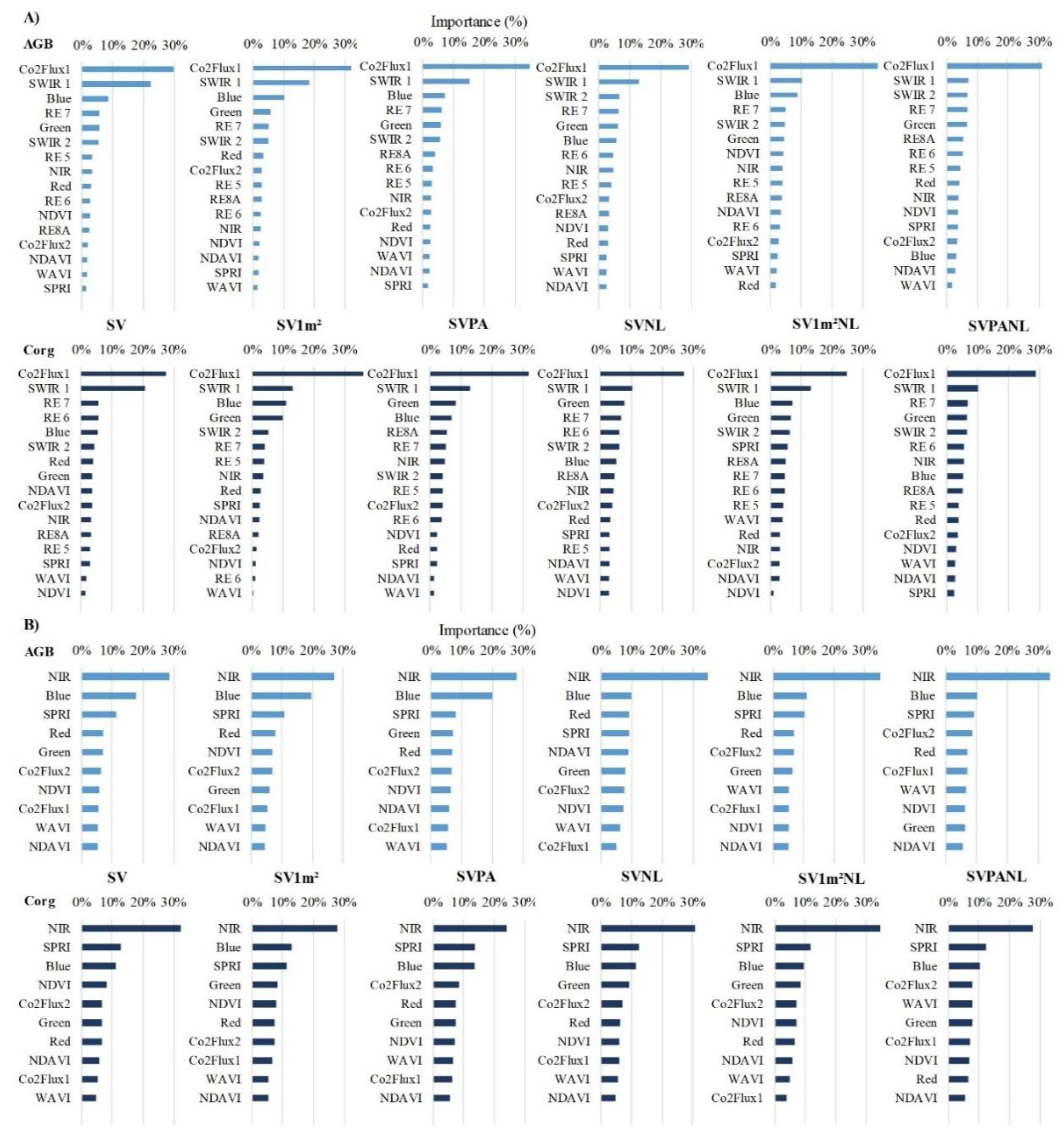
3.3. Importance of Predictor Variables

Figure 6 shows the importance of predictor variables for the final optimized models. We expected the VIs to predominate as the most important variables for the models in both sensors, but our results were different. Although at least one VI was present among the five most important variables in all the models, the single-bands were present in greater quantity, indicating that they have abundant information to the performance of models in estimating AGB and Corg.
The two most important variables in the S2 models were VI CO²Flux1, followed by the band SWIR and this order of importance was maintained in all the AGB and Corg models. For the PS models, the band NIR was the most important variable, followed by Blue band in the AGB models and VI SPRI in the Corg models.
For both sensors, the models with Group 2 treatments (NL) inclined to centralize the importance in the first variable, while the Group 1 models (without NL) better divided the importance between the first five variables. As a result, this set of the 5 most important variables has higher importance values in the Group 1 models (from 65% to 74%) than in Group 2 (57% to 71%). We also found that these most important variables differed in the AGB and Corg models and between the respective treatments.
Spatial modeling of AGB and Corg was performed for the top-performing models per sensor (Figure 7) and for all models in the in the Supplementary Figures (Figure S1 and S2). RF predictions using S2 and PS data showed divergent spatial distribution trends. In the area highlighted in Figure 7, where sampling occurred, AGB and Corg values were similar for S2 and PS across treatments, with comparable spatial distribution. However, in the central Cyperus boundary area, characterized by less human disturbance and higher moisture, predicted values were lower with S2 data (Figure S1 and S2), with little spatial heterogeneity (range: AGB 758 to 907 g/m², Corg 293 to 381 g/m²), while for PS (range: AGB 643 to 954 g/m², Corg 270 to 403 g/m²). The PS models’ highest values are found in areas with woody and shrub species, transition zones, and wet fields, while in the S2 models, they are found in cultivated areas. The lowest values are observed in regions with higher moisture or open water.
Despite the maximum values of AGB and Corg being higher in the S2 models, the ranges of predicted values within the same treatment were greater with PS data (Figure S1 and S2). For instance, in the SV and SV1m² treatments, the range values were 10 g and 41 g higher for AGB, respectively.

4. Discussion

4.1. AGB and Corg Estimation Accuracy and Efficiency of Sensors

The most accurate estimates were achieved with the S2 models, with RMSE OOB (validation) between 19.7% and 22.7% of the mean observed data, while the PS models ranged between 21% and 35.9%. The best S2 AGB and Corg models achieved R² of 0.87 and 0.89 and RMSE% OOB of 1.71% and 19.71%, respectively. These mean validation error values are similar to those achieved in recent studies using RF and Sentinel 2 in predicting AGB of wetlands with similar herbaceous vegetation: 15% [16], 25% [15], and 22.35% [65] for Mangrove vegetation.
When compared to a study who used the same sensors and Linear Multiple Regression to estimate AGB and Corg of Scirpus giganteus in Banhado Grande [39] (respectively R² = 0.46 and 0.45; RMSE = 166.73 g/m² and 67.47 g/m²), the RF results were better with S2 data (R² = 0.85 and 0.79; RMSE = 157.26 g/m² and 57.38 g/m²). This can be attributed to its ability to capture complex non-linear relationships between vegetation and RS information [16], and in general, ML methods have shown better performance than linear methods in wetlands [7,16,18,29].
Wetlands research has not yet extensively utilized the PS sensor. Among these, linear regressions was used to estimate mangrove biomass [66], finding S2 and PS sensors produced models with R² of 0.89 and 0.80, respectively. The authors suggest that PS’s lower VIs may have reduced model accuracy compared to RapidEye and S2 sensors. Lower VIs for PS are also reported in other studies [39], this may have contributed to the lower performance of our PS RF models. S2’s superior accuracy in assessing Spartina alterniflora phenological heterogeneity [67], though both satellites had comparable metrics (R² 0.63), the PS providing greater spatial detail in phenology and biomass.
Although PS images provide fine detail in VIs and biomass, the complexity of VIs trajectories can lead to greater errors in models [8]. The Figure 7 and Supplementary Figures (S1 and S2) illustrate PS models’ clearer AGB and Corg variations compared to S2, yet S2 surpasses in prediction accuracy. Performance metrics are similar, but S2’s are superior. Spectral prediction model differences may stem from variations in radiometric quality, pixel size, and bandwidth, that is, band range in nm [68]. The spectral consistency between sensors improves with greater between band wavelength overlap [69]. Here, S2’s Blue and NIR bands are broader than PS’s, and S2 includes additional SWIR and Red edge bands.
Studies comparing PS and S2 sensors, among others, with different spatial resolutions for predicting AGB and Corg, indicate that spectral and temporal information is more relevant than high spatial resolution. Thus, images with larger pixels provide more accurate estimates [70,71] because they capture a larger area of reflectance, reducing variations in climate, angle of incidence and other sources of potential error between satellites [68].
The R² values, although high during model training (between 0.80 and 0.89), decreased in the OOB datasets (between 0.15 and 0.29), suggesting a need for additional input variables to understand generalization. Nonetheless, our OOB R² values exceed those for validation sets from similar RF regression studies in wetlands. An R² of 0.14 was reported for the validation dataset using bands and VIs [65], which in-creased to 0.74 using their mean, median, and percentile values. Incorporating these metrics could thus enhance RF model precision for AGB and Corg estimation in marshes with scarce field data.

4.2. The Effect of Treatments and Plots Size on Model Performance and Importance of Spectral Variables

Our tests with prediction models using different treatments indicated that the transformation of the data into a NL (G2) contributed to an improvement in the performance of the models. The models with G2 treatments achieved, in sum, R² values slightly higher (0.08) than the untransformed ones (G1), Table 4. The transformation of the data also reflected on the effect of the variation of the plot size on the performance of the models, explaining between 46% and 89% of the variation between the root mean square error percentage (RMSE%) and plot size (Figure 5). It also tended to centralize importance on the most important spectral variable, this indicates that G2 models depend heavily on one or a few predictors, while G1 models allow the distribution of importance to a wider range of variables.
An NL transformation was applied to soil Corg for input into prediction models, including RF [23]. This reduces the variability of the data for more stable training. The NL transformation is effective when proportional variations of the dependent variable produce linear variations of the independent variable [72], aligning with the AGB-Corg relationship and PS and S2 predictors [15,39].
Additionally, in estimating AGB and Corg content in mangrove species, was observed that the NL transformation mitigates the increasing AGB variance with increasing tree size or canopy structure, thus reducing heteroscedasticity [73]. By evaluating linear models with and without NL transformation, the author found that NL models more accurately reflect the biomass-independent variable relationship, supporting with [74] and our findings.
Regarding the effects of plot size on model performance, generally, treatments estimated to the sensor Pixel Area performed better in AGB predictions and Sample Value treatments performed better in Corg predictions. By normalizing the data and mitigate the variance, the treatments in G2 revealed the hidden relationship in G1 between plot size and model performance. This made it noticeable that the prediction errors (RMSE%) of the models decrease with the increase in the plot size with the S2 sensor data. In the models with PS data, the test with larger plots did not have the same effect (Figure 5).
Research on AGB and Corg prediction has shown that plot size and sample number affect model performance, particularly in forest ecosystems, planted forests, and mangroves with use of Lidar and other sensors, is noted for reducing model errors as plot size increases [22,31,32,33,75]. As factors that may contribute to this observation, larger plots mitigate co-registration errors due to increased spatial overlap, enhancing resilience to GPS positioning errors and reducing spatial variance among plots [25,33].
The way in which plot and sample sizes affect RF model accuracy was examined using Pléiades sensor data (spatial resolution from 50 cm to 2 m) in plantation forests in Iran [76]. Larger plots (300 m² and 500 m²) yielded marginally higher accuracies (RMSE% ~ 0.51 to 0.65) compared to 100 m² plots (RMSE% ~ 0.59 to 0.70). However, factors like sample size and total area sampled had a more pronounced impact on performance. These results do not suggest a clear advantage of preferred plot size for precise AGB estimates, though, they propose us for exploring additional factors to enhance PS model performance.
Without comparable studies on plot size effects in wetland AGB and Corg models with herbaceous vegetation, our results align to those based on forest and other vegetation cover estimates. Larger plots improve S2 model performance (Figure 5A and 5B), suggesting that smaller plots may compromise the reliability of estimates.
Predictor variables’ importance varied across treatments on the same sensor, indicating that their correlations with the dependent variables differ between treatments. Nonetheless, a consistent pattern was observed in the top five variables, involving bands and VIs (Figure 6). CO2Flux VI and SWIR bands 1 and 2, Blue, Green, and RE 6 and 7 (for S2 data), along with NIR, Blue, Red, Green bands, and SPRI and CO2Flux VIs (for PS data), were the most effective predictors for precise AGB and Corg models.
CO2Flux, traditionally linked with hyperspectral data, has been successfully applied to multispectral images by substituting the bands centered on 531 nm and 570 nm with blue and green bands, as shown in various studies [77,78,79]. The CO2Flux, when adapted to PS and S2 images, reliably provides a carbon flux estimate comparable to hyperspectral sensors [78].
The CO2Flux was utilized in the context of extreme wetland events with S2 data to evaluate ecosystem service losses in hailstorm-affected mangroves [77]. The authors confirmed the VI’s effectiveness in gauging storm impact on carbon storage. Similarly, the SPRI’s effectiveness was validated in measuring Corg storage under drought-induced water stress [80].
Carbon flux-related VIs, specifically CO2Flux 1 and 2 and SPRI, have surpassed traditional indices like NDVI and NDAVI in importance. The SPRI to be more sensitive to daily and seasonal carbon flux changes in mangroves, while NDVI proved to be stable in perennial mangroves [54]. The spectral mixing’s impact on CO2Flux, since SPRI were lower in high-resolution sensors, such as PlanetScope and AisaFENIX, underscoring CO2Flux’s importance with S2 data [78]. Additionally, CO2Flux2’s importance in PS models can be attributed to NDAVI’s resistance to background influences (moist soil and litter) [49], greater in PS for the vegetation studied [39].
SWIR bands effectively capture vegetation signals and are at the top of the important variables in ML models for AGB and Corg in wetlands, as evidenced by S2 data [81], Landsat OLI [18], and others [82]. These sensors discern vegetation and soil moisture content [83], showing a positive correlation with vegetation and a negative one with soil moisture [84]. Spatial predictions (Figure 7, S1 and S2 in the Supplementary Figures) show lower AGB and Corg with S2, likely due to SWIR’s humidity sensitivity, yet without compromising S2 model accuracy.
Visible bands (Blue/Red for PS, Blue/Green for S2) and red edge (RE6 and 7) were important due to their absorption by vegetation pigments like carotenoids, xanthophylls and chlorophyll, indicating photosynthetic activity [51,52]. This absorption inversely relates to NIR spectral response, which rises with AGB [85]. These bands, including in VIs, correlate strongly with AGB and Corg in herbaceous wetlands [15,16,29].
This study initially explored important research gaps in the modeling of AGB and Corg in herbaceous wetlands. We examined the influence of data normalization on the performance of RF models in estimating AGB and Corg, an area not previously explored, and found that models with normalized input data had lower estimation errors in the majority. The NL transformation is frequently utilized in allometric equations for AGB and Corg inventories [22,86]. Pixel values of AGB and Corg in NL can be used for these purposes and others mentioned, with an option to revert to original values via the exponential inverse function.
In light of the absence of research on the influence of sample plot size on the accuracy of AGB and Corg estimation models in herbaceous marshes, we made progress in addressing this issue and found that the estimation errors decrease as the S2 model plot size increases. Our findings also show that OOB estimates are efficient for validation, yielding average prediction errors similar to those of validation sets in reference studies. This can reduce the need for extensive collection, addressing the challenges of access and collecting enough wetland biomass for the test and validation set, emphasizing that this was a significant difficulty in study.
These findings have the potential to guide the standardization of input data collection and treatment in predictive models based on RS and ML in wetlands, aiming for consistency in predictions for herbaceous wetland inventories and monitoring.
While these are important findings, validation is necessary for other wetland types and RS data types. Additional factors, such as the number of samples and total area sampled, can be explored to further improve the estimation model's performance. Multi-source data fusion, including climatic and elevation data, can refine the model's predictive capabilities [17]. We therefore encourage further studies on this subject.

5. Conclusions

We utilized an optimized RF regression model based on PS and S2 optical sensor data and field collection to estimate in a wetland AGB and Corg in southern Brazil. Model efficacy was assessed against field data treatments, including variations in plot size and data normalization. Sensors accuracy and key spectral indicators for AGB and Corg were also evaluated. Our results lead to the following conclusions:
  • Regarding RF parameters, different Ntrees impacted model errors, notably in non-normalized treatments, enhancing RF model precision. Thus, optimized RF models provide more accurate estimates. OOB estimates served effectively for validation, with average prediction errors within the limits found in validation sets in reference studies. This result is useful amidst wetland data collection challenges;
  • Normalized sample data treatments enhanced RF model accuracy for AGB and Corg prediction. Estimation errors decrease as S2 model plot size increased, indicating smaller plots may compromise estimate reliability with S2;
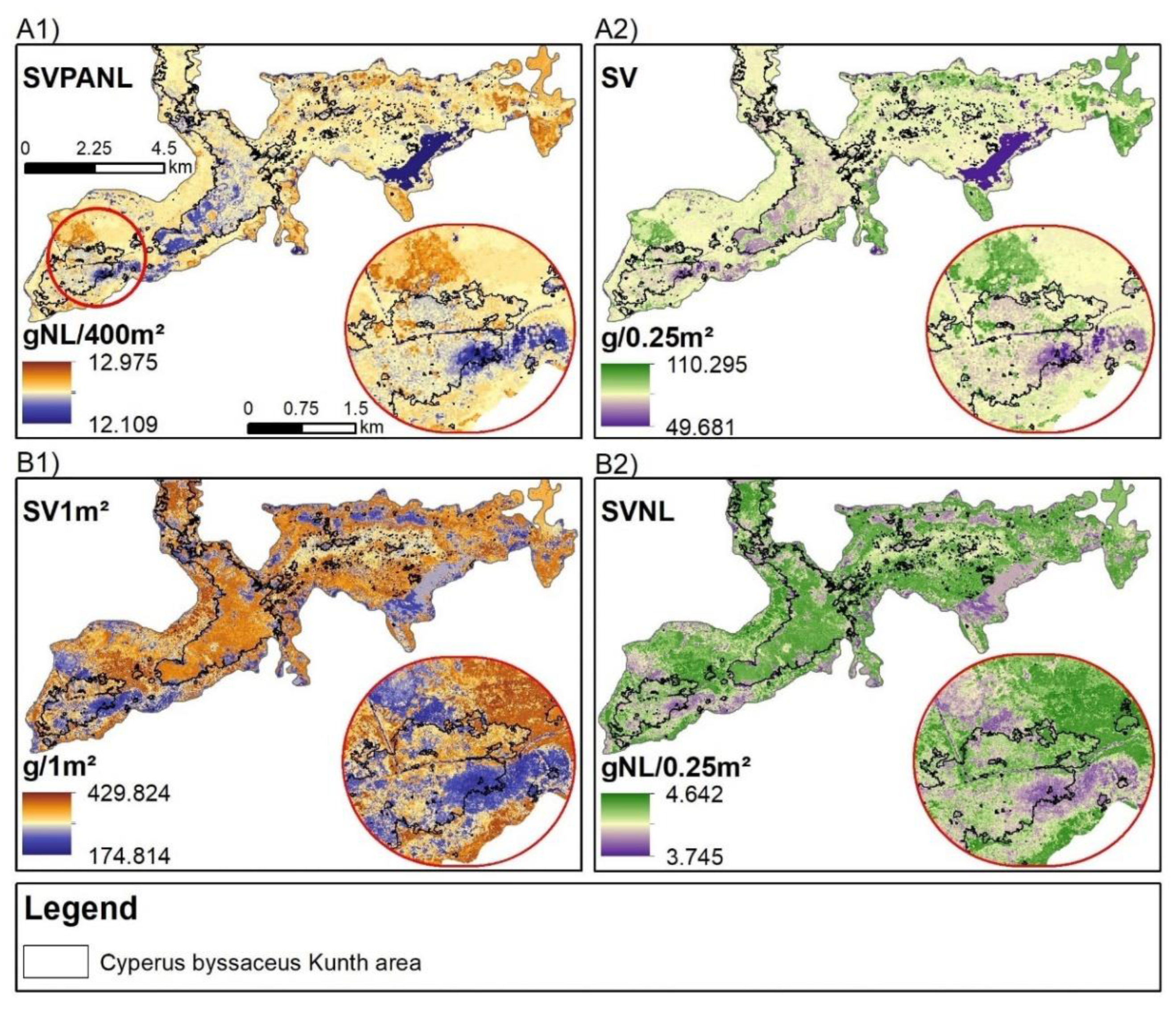
  • Utilizing S2 and PS sensors underscored, respectively, the value of medium spatial resolution satellite data for enhancing estimate accuracy and high-resolution data for delineating AGB and Corg spatial variability in wetlands. Sensors performance were close, however, S2 was more efficient;
  • The RF method, employing the combination of VI CO2Flux and S2’s SWIR, Blue, Green, and RE bands 6 and 7 as predictors, excelled in AGB and Corg prediction. Leveraging an ML algorithm with VI and bands indicative of carbon fluxes and biomass changes proved beneficial, and these predictors serve as spectral indicators of these ecological functions;
  • In addition to optimizing the parameters of the RF model, optimizing the input set of AGB and Corg collected in the field, i.e., evaluating normalization and plot sizes, has contributed to more accurate estimates. This approach holds promise for improved monitoring of the ecological processes of AGB and Corg storage in wetlands and for contributing to the understanding of these ecosystems as carbon sinks, vital for offsetting emissions and meeting national and global GHG reduction targets;
  • We encourage future work that compares the effects of different plot sizes, sample data normalization methods, sensors, and VIs in RF models and other ML approaches on the accuracy of AGB and Corg estimates in marshes, as well as in other wetlands with emergent herbaceous vegetation, such as salt marshes and peatlands. This will contribute to the continued advancement of knowledge on improving the modeling of AGB and Corg in wetlands.

Supplementary Materials

The following supporting information can be downloaded at the website of this paper posted on Preprints.org.

Author Contributions

Tássia Belloli: Writing: Original Draft, Conceptualization, Methodology, Investigation, Formal analysis, Visualization. Laurindo Guasselli: Conceptualization; Writing - Review & Editing, Supervision, Funding acquisition. Diniz Arruda: Methodology and software, Writing - Review & Editing, Carina Korb and Christhian Cunha: Writing - Review & Editing.

Data Availability Statement

The datasets analyzed in this study can be found in Copernicus Open Access Hub and Planet Research and Education Programme on the Planet Explorer website. Further inquiries about the data can be directed to the corresponding author.

Acknowledgments

The authors would like to thank the Gravataí Municipal Environment Foundation for Support to the field work and the aerial photos granted. This study was financed in part by the Coordenação de Aperfeiçoamento de Pessoal de Nível Superior – Brasil (CAPES) – Finance Code 001, Award no. 88887.488339/2020-00, and Rio Grande do Sul state Foundation for Research Support (FAPERGS).

Conflicts of Interest

The authors declare no conflict of interest.

References

  1. Barbier, E.B.; Hacker, S.D.; Kennedy, C.; Koch, E.W.; Stier, A.C.; Silliman, B.R. The Value of Estuarine and Coastal Ecosystem Services. Ecol. Monogr. 2011, 81, 169–193. [Google Scholar] [CrossRef]
  2. Hiraishi, T.; Krug, T.; Tanabe, K.; Srivastava, N.; Baasansuren, J.; Fukuda, M.; Troxler, T.G. 2013 Supplement to the 2006 IPCC Guidelines for National Greenhouse Gas Inventories: Wetlands. IPCC Switz. 2014, Available online: https://tinyurl.com/5c4xm8rp.
  3. Webb, E.L.; Friess, D.A.; Krauss, K.W.; Cahoon, D.R.; Guntenspergen, G.R.; Phelps, J. A Global Standard for Monitoring Coastal Wetland Vulnerability to Accelerated Sea-Level Rise. Nat. Clim. Change 2013, 3, 458–465. [Google Scholar] [CrossRef]
  4. Rice, J.; Seixas, C.; Elena, M.; Bedoya, M.; Valderrama, N.; Anderson, C. Resumen Para Los Responsables de La Formulación de Políticas Del Informe de Evaluación Regional Sobre Diversidad Biológica y Servicios de Los Ecosistemas Para Las Américas de La Plataforma Intergubernamental Científico-Normativa Sobre Diversidad Biológica. Plataforma Intergub. Científico-Norm. Dobre Divers. Biológica Serv. Los Ecosistemas 2018, 34, Available online: https://tinyurl.com/4seyyrds.
  5. Poulter, B.; Fluet-Chouinard, E.; Hugelius, G.; Koven, C.; Fatoyinbo, L.; Page, S.E.; Rosentreter, J.A.; Smart, L.S.; Taillie, P.J.; Thomas, N.; et al. A Review of Global Wetland Carbon Stocks and Management Challenges. In Geophysical Monograph Series; Krauss, K.W., Zhu, Z., Stagg, C.L., Eds.; Wiley, 2021; pp. 1–20 ISBN 978-1-119-63928-2. [CrossRef]
  6. Byrd, K.B.; Ballanti, L.; Thomas, N.; Nguyen, D.; Holmquist, J.R.; Simard, M.; Windham-Myers, L. A Remote Sensing-Based Model of Tidal Marsh Aboveground Carbon Stocks for the Conterminous United States. ISPRS J. Photogramm. Remote Sens. 2018, 139, 255–271. [Google Scholar] [CrossRef]
  7. Ren, Y.; Mao, D.; Li, X.; Wang, Z.; Xi, Y.; Feng, K. Aboveground Biomass of Marshes in Northeast China: Spatial Pattern and Annual Changes Responding to Climate Change. Front. Ecol. Evol. 2022, 10, 1043811. [Google Scholar] [CrossRef]
  8. Dronova, I.; Taddeo, S.; Hemes, K.S.; Knox, S.H.; Valach, A.; Oikawa, P.Y.; Kasak, K.; Baldocchi, D.D. Remotely Sensed Phenological Heterogeneity of Restored Wetlands: Linking Vegetation Structure and Function. Agric. For. Meteorol. 2021, 296, 108215. [Google Scholar] [CrossRef]
  9. Campbell, A.D.; Temilola Fatoyinbo, L.; Charles, S.; Bourgeau-Chavez, L.L. A Review of Carbon Monitoring in Wet Carbon Systems Using Remote Sensing. Environ. Res. Lett. 2022, 17, 025009. [Google Scholar] [CrossRef]
  10. Requena-Mullor, J.M.; Reyes, A.; Escribano, P.; Cabello, J. Assessment of Ecosystem Functioning from Space: Advancements in the Habitats Directive Implementation. Ecol. Indic. 2018, 89, 893–902. [Google Scholar] [CrossRef]
  11. Cabello, J.; Fernández, N.; Alcaraz-Segura, D.; Oyonarte, C.; Piñeiro, G.; Altesor, A.; Delibes, M.; Paruelo, J.M. The Ecosystem Functioning Dimension in Conservation: Insights from Remote Sensing. Biodivers. Conserv. 2012, 21, 3287–3305. [Google Scholar] [CrossRef]
  12. Alcaraz-Segura, D.; Lomba, A.; Sousa-Silva, R.; Nieto-Lugilde, D.; Alves, P.; Georges, D.; Vicente, J.R.; Honrado, J.P. Potential of Satellite-Derived Ecosystem Functional Attributes to Anticipate Species Range Shifts. Int. J. Appl. Earth Obs. Geoinformation 2017, 57, 86–92. [Google Scholar] [CrossRef]
  13. Miller, G.J.; Morris, J.T.; Wang, C. Estimating Aboveground Biomass and Its Spatial Distribution in Coastal Wetlands Utilizing Planet Multispectral Imagery. Remote Sens. 2019, 11, 2020. [Google Scholar] [CrossRef]
  14. Warwick-Champion, E.; Davies, K.P.; Barber, P.; Hardy, N.; Bruce, E. Characterising the Aboveground Carbon Content of Saltmarsh in Jervis Bay, NSW, Using ArborCam and PlanetScope. Remote Sens. 2022, 14, 1782. [Google Scholar] [CrossRef]
  15. Zhao, Y.; Mao, D.; Zhang, D.; Wang, Z.; Du, B.; Yan, H.; Qiu, Z.; Feng, K.; Wang, J.; Jia, M. Mapping Phragmites Australis Aboveground Biomass in the Momoge Wetland Ramsar Site Based on Sentinel-1/2 Images. Remote Sens. 2022, 14, 694. [Google Scholar] [CrossRef]
  16. Li, C.; Zhou, L.; Xu, W. Estimating Aboveground Biomass Using Sentinel-2 MSI Data and Ensemble Algorithms for Grassland in the Shengjin Lake Wetland, China. Remote Sens. 2021, 13, 1595. [Google Scholar] [CrossRef]
  17. Cai, F.; Tang, B.-H.; Ji, X.; Huang, L.; Fu, Z.; Fan, D. Predicting Carbon Storage in the Yunnan-Kweichow Plateau Wetlands Using a Fusion of Multi-Source Remote Sensing Data and Machine Learning. In Proceedings of the IGARSS 2024 - 2024 IEEE International Geoscience and Remote Sensing Symposium; July 2024; pp. 4806–4809. [Google Scholar] [CrossRef]
  18. Wan, R.; Wang, P.; Wang, X.; Yao, X.; Dai, X. Modeling Wetland Aboveground Biomass in the Poyang Lake National Nature Reserve Using Machine Learning Algorithms and Landsat-8 Imagery. J. Appl. Remote Sens. 2018, 12, 046029. [Google Scholar] [CrossRef]
  19. Cutler, D.R.; Edwards Jr., T. C.; Beard, K.H.; Cutler, A.; Hess, K.T.; Gibson, J.; Lawler, J.J. Random Forests for Classification in Ecology. Ecology 2007, 88, 2783–2792. [Google Scholar] [CrossRef]
  20. Da Silva, J.V.S. Aprendizado de Máquinas Por “Random Forest” Para a Modelagem Da Altura de Árvores de Seringueira. Term paper, Universidade Federal de Mato Grosso do Sul: Mato Grosso do Sul, 2023, Available online:https://repositorio.ufms.br/handle/123456789/8264.
  21. Nishiwaki, A.A.M. Uso do LIDAR e a potencialidade de geração de renda mediante pagamento por serviço ambiental de sequestro de carbono em floresta tropical sazonalmente seca. Doctoral dissertation, Federal University of Pernambuco: Pernambuco, 2023, Available online: https://repositorio.ufpe.br/handle/123456789/52100.
  22. Rocha de Souza Pereira, F.; Kampel, M.; Gomes Soares, M.L.; Estrada, G.C.D.; Bentz, C.; Vincent, G. Reducing Uncertainty in Mapping of Mangrove Aboveground Biomass Using Airborne Discrete Return Lidar Data. Remote Sens. 2018, 10, 637. [Google Scholar] [CrossRef]
  23. Chan, C.K.; Gomez, C.A.; Kothikar, A.; Baiz-Villafranca, P.M. Satellite-Based Carbon Estimation in Scotland: AGB and SOC. Land 2023, 12, 818. [Google Scholar] [CrossRef]
  24. Mahmud Sujon, K.; Binti Hassan, R.; Tusnia Towshi, Z.; Othman, M.A.; Abdus Samad, M.; Choi, K. When to Use Standardization and Normalization: Empirical Evidence From Machine Learning Models and XAI. IEEE Access 2024, 12, 135300–135314. [Google Scholar] [CrossRef]
  25. Frazer, G.W.; Magnussen, S.; Wulder, M.A.; Niemann, K.O. Simulated Impact of Sample Plot Size and Co-Registration Error on the Accuracy and Uncertainty of LiDAR-Derived Estimates of Forest Stand Biomass. Remote Sens. Environ. 2011, 115, 636–649. [Google Scholar] [CrossRef]
  26. Dai, X.; Yang, G.; Liu, D.; Wan, R. Vegetation Carbon Sequestration Mapping in Herbaceous Wetlands by Using a MODIS EVI Time-Series Data Set: A Case in Poyang Lake Wetland, China. Remote Sens. 2020, 12, 3000. [Google Scholar] [CrossRef]
  27. Sun, S.; Wang, Y.; Song, Z.; Chen, C.; Zhang, Y.; Chen, X.; Chen, W.; Yuan, W.; Wu, X.; Ran, X.; et al. Modelling Aboveground Biomass Carbon Stock of the Bohai Rim Coastal Wetlands by Integrating Remote Sensing, Terrain, and Climate Data. Remote Sens. 2021, 13, 4321. [Google Scholar] [CrossRef]
  28. Adam, E.; Mutanga, O.; Abdel-Rahman, E.M.; Ismail, R. Estimating Standing Biomass in Papyrus (Cyperus Papyrus L.) Swamp: Exploratory of in Situ Hyperspectral Indices and Random Forest Regression. Int. J. Remote Sens. 2014, 35, 693–714. [Google Scholar] [CrossRef]
  29. Mutanga, O.; Adam, E.; Cho, M.A. High Density Biomass Estimation for Wetland Vegetation Using WorldView-2 Imagery and Random Forest Regression Algorithm. Int. J. Appl. Earth Obs. Geoinformation 2012, 18, 399–406. [Google Scholar] [CrossRef]
  30. Naidoo, L.; van Deventer, H.; Ramoelo, A.; Mathieu, R.; Nondlazi, B.; Gangat, R. Estimating above Ground Biomass as an Indicator of Carbon Storage in Vegetated Wetlands of the Grassland Biome of South Africa. Int. J. Appl. Earth Obs. Geoinformation 2019, 78, 118–129. [Google Scholar] [CrossRef]
  31. Zolkos, S.G.; Goetz, S.J.; Dubayah, R. A Meta-Analysis of Terrestrial Aboveground Biomass Estimation Using Lidar Remote Sensing. Remote Sens. Environ. 2013, 128, 289–298. [Google Scholar] [CrossRef]
  32. Wang, D.; Wan, B.; Liu, J.; Su, Y.; Guo, Q.; Qiu, P.; Wu, X. Estimating Aboveground Biomass of the Mangrove Forests on Northeast Hainan Island in China Using an Upscaling Method from Field Plots, UAV-LiDAR Data and Sentinel-2 Imagery. Int. J. Appl. Earth Obs. Geoinformation 2020, 85, 101986. [Google Scholar] [CrossRef]
  33. Qiu, B.; Li, S.; Cao, J.; Zhang, J.; Yang, K.; Luo, K.; Huang, K.; Jiang, X. Uncertainty Analysis of Forest Aboveground Carbon Stock Estimation Combining Sentinel-1 and Sentinel-2 Images. Forests 2024, 15, 2134. [Google Scholar] [CrossRef]
  34. Simioni, J.P.D.; Guasselli, L.A.; Etchelar, C.B. Connectivity among Wetlands of EPA of Banhado Grande, RS. RBRH 2017, 22. [Google Scholar] [CrossRef]
  35. Accordi, I.; Hartz, S.; ohlweiler, Adalberto, O. O Sistema Banhado Grande Como Uma Área Úmida de Importância Internacional.; Simpósio de áreas protegidas, Pelotas, Brazil, September 1 2003, Available online: https://tinyurl.com/79aeekcv.
  36. Serviço Geológico Do Brasil - CPRM - GeoSGB. Available online: https://geoportal.sgb.gov.br/geosgb/ (accessed on 17 January 2025).
  37. Rossato, M.S. Os Climas Do Rio Grande Do Sul: Uma Proposta de Classificação Climática. Entre-Lugar 2020, 11, 57–85. [Google Scholar] [CrossRef]
  38. Pereira-Silva, L.; Trevisan, R.; Rodrigues, A.C.; Larridon, I. Combining the Small South American Genus Androtrichum into Cyperus (Cyperaceae). Plant Ecol. Evol. 2020, 153, 446–454. [Google Scholar] [CrossRef]
  39. Belloli, T.F.; Guasselli, L.A.; Kuplich, T.M.; Ruiz, L.F.C.; de Arruda, D.C.; Etchelar, C.B.; Simioni, J.D. Estimation of Aboveground Biomass and Carbon in Palustrine Wetland Using Bands and Multispectral Indices Derived from Optical Satellite Imageries PlanetScope and Sentinel-2A. J. Appl. Remote Sens. 2022, 16, 034516–034516. [Google Scholar] [CrossRef]
  40. Frantz, D.S.; Carraro, C.C.; Verdum, R.; Garcia, M. Caracterização de Ambientes Paludais Da Planície Costeira Do Rio Grande Do Sul Em Imagens Orbitais TM/Landsat 5.; Manaus, Brazil, 1990; Vol. 6, pp. 408–418. Available online: https://tinyurl.com/34hp6zej.
  41. Irgang, B.E.; Júnior, G.; de Senna Gastal Jr, C.V. Macrófitas Aquáticas Da Planície Costeira Do RS; UFRGS, 1996.
  42. Pratolongo, P.; Kandus, P. Dinámica Biomasa Aérea En Pajonales Scirpus Giganteus Juncales Schoenoplectus Californicus En Zona Front. Bajo Delta Río Paraná Argent. Ecotrópicos. 2005, 18, 30–37. [Google Scholar]
  43. Howard, J.; Hoyt, S.; Isensee, K; Telszewski, M; Pidgeon, E Coastal Blue Carbon: Methods for Assessing Carbon Stocks and Emissions Factors in Mangroves, Tidal Salt Marshes, and Seagrass Meadows; Arlington, Virginia, USA, 2014.
  44. Pompêo, M.L.M.; Moschini, C.V. Biomassa Das Macrófitas Aquáticas: O Método Do Quadro; RiMa São Carlos, SP, 2003.
  45. Sifleet, S.; Pendleton, L.; Murray, B.C. State of the Science on Coastal Blue Carbon: A Summary for Policy Makers. Available online: https://nicholasinstitute.duke.edu/sites/default/files/publications/state-of-science-coastal-blue-carbon-paper.pdf (accessed on 17 January 2025).
  46. Main-Knorn, M.; Pflug, B.; Louis, J.; Debaecker, V.; Müller-Wilm, U.; Gascon, F. Sen2Cor for Sentinel-2. Proc. SPIE 2017, 10427, 1042704. [Google Scholar] [CrossRef]
  47. Planet Imagery Product Specification. Available online: https://assets.planet.com/docs/Planet_Combined_Imagery_Product_Specs_letter_screen.pdf (accessed on 17 January 2025).
  48. Rouse, J.W.; Haas, R.H.; Deering, D.W.; Schell, J.A.; Harlan, J.C. Monitoring the Vernal Advancement and Retrogradation (Green Wave Effect) of Natural Vegetation; Texas A&M Univ. College Station, TX, United States, 1974; Available online: https://ntrs.nasa.gov/citations/19750020419.
  49. Villa, P.; Laini, A.; Bresciani, M.; Bolpagni, R. A Remote Sensing Approach to Monitor the Conservation Status of Lacustrine Phragmites Australis Beds. Wetl. Ecol. Manag. 2013, 21, 399–416. [Google Scholar] [CrossRef]
  50. Villa, P.; Bresciani, M.; Braga, F.; Bolpagni, R. Comparative Assessment of Broadband Vegetation Indices Over Aquatic Vegetation. IEEE J. Sel. Top. Appl. Earth Obs. Remote Sens. 2014, 7, 3117–3127. [Google Scholar] [CrossRef]
  51. Gamon, J.A.; Serrano, L.; Surfus, J.S. The Photochemical Reflectance Index: An Optical Indicator of Photosynthetic Radiation Use Efficiency across Species, Functional Types, and Nutrient Levels. Oecologia 1997, 112, 492–501. [Google Scholar] [CrossRef]
  52. Rahman, A.F.; Gamon, J.A.; Fuentes, D.A.; Roberts, D.A.; Prentiss, D. Modeling Spatially Distributed Ecosystem Flux of Boreal Forest Using Hyperspectral Indices from AVIRIS Imagery. J. Geophys. Res. Atmospheres 2001, 106, 33579–33591. [Google Scholar] [CrossRef]
  53. Baptista, G. Validação Da Modelagem de Seqüestro de Carbono Para Ambientes Tropicais de Cerrado, Por Meio de Dados AVIRIS e Hyperion. In Proceedings of the Anais XI SBSR; INPE: Belo Horizonte, 2003; pp. 1037–1044. [Google Scholar]
  54. Zhu, X.; Song, L.; Weng, Q.; Huang, G. Linking In Situ Photochemical Reflectance Index Measurements With Mangrove Carbon Dynamics in a Subtropical Coastal Wetland. J. Geophys. Res. Biogeosciences 2019, 124, 1714–1730. [Google Scholar] [CrossRef]
  55. Mohanty, P.C.; Shetty, S.; Mahendra, R.S.; Nayak, R.K.; Sharma, L.K.; Rama Rao, E.P. Spatio-Temporal Changes of Mangrove Cover and Its Impact on Bio-Carbon Flux along the West Bengal Coast, Northeast Coast of India. Eur. J. Remote Sens. 2021, 54, 525–537. [Google Scholar] [CrossRef]
  56. Liu, Y.; Wu, C.; Tian, F.; Wang, X.; Gamon, J.A.; Wong, C.Y.S.; Zhang, X.; Gonsamo, A.; Jassal, R.S. Modeling Plant Phenology by MODIS Derived Photochemical Reflectance Index (PRI). Agric. For. Meteorol. 2022, 324, 109095. [Google Scholar] [CrossRef]
  57. Breiman, L. Random Forests. Mach. Learn. 2001, 45, 5–32. [Google Scholar] [CrossRef]
  58. Pedregosa, F.; Pedregosa, F.; Varoquaux, G.; Varoquaux, G.; Org, N.; Gramfort, A.; Gramfort, A.; Michel, V.; Michel, V.; Fr, L.; et al. Scikit-Learn: Machine Learning in Python. J. Mach. Learn. Res. 2011, 12, 2825–2830. [Google Scholar]
  59. Guerini Filho, M.; Kuplich, T.M.; Quadros, F.L.F.D. Estimating Natural Grassland Biomass by Vegetation Indices Using Sentinel 2 Remote Sensing Data. Int. J. Remote Sens. 2020, 41, 2861–2876. [Google Scholar] [CrossRef]
  60. Morris, J.D.; Daood, S.S.; Nimmo, W. Machine Learning Prediction and Analysis of Commercial Wood Fuel Blends Used in a Typical Biomass Power Station. Fuel 2022, 316, 123364. [Google Scholar] [CrossRef]
  61. Xing, J.; Luo, K.; Wang, H.; Fan, J. Estimating Biomass Major Chemical Constituents from Ultimate Analysis Using a Random Forest Model. Bioresour. Technol. 2019, 288, 121541. [Google Scholar] [CrossRef]
  62. Valbuena, R.; Hernando, A.; Manzanera, J.A.; Görgens, E.B.; Almeida, D.R.A.; Silva, C.A.; García-Abril, A. Evaluating Observed versus Predicted Forest Biomass: R-Squared, Index of Agreement or Maximal Information Coefficient? Eur. J. Remote Sens. 2019, 52, 345–358. [Google Scholar] [CrossRef]
  63. Mauya, E.W.; Madundo, S. Modelling Above Ground Biomass Using Sentinel 2 and Planet Scope Data in Dense Tropical Montane Forests of Tanzania. Tanzan. J. For. Nat. Conserv. 2022, 91, 132–153. [Google Scholar]
  64. Lawrence, R.L.; Wood, S.D.; Sheley, R.L. Mapping Invasive Plants Using Hyperspectral Imagery and Breiman Cutler Classifications (randomForest). Remote Sens. Environ. 2006, 100, 356–362. [Google Scholar] [CrossRef]
  65. Ghosh, S.M.; Behera, M.D.; Jagadish, B.; Das, A.K.; Mishra, D.R. A Novel Approach for Estimation of Aboveground Biomass of a Carbon-Rich Mangrove Site in India. J. Environ. Manage. 2021, 292, 112816. [Google Scholar] [CrossRef]
  66. Baloloy, A.B.; Blanco, A.C.; Candido, C.G.; Argamosa, R.J.L.; Dumalag, J.B.L.C.; Dimapilis, L.L.C.; Paringit, E.C. Estimation of Mangrove Forest Aboveground Biomass Using Multispectral Bands, Vegetation Indices and Biophysical Variables Derived from Optical Satellite Imageries: Rapideye, Planetscope and Sentinel-2. ISPRS Ann. Photogramm. Remote Sens. Spat. Inf. Sci. 2018, IV–3, 29–36. [Google Scholar] [CrossRef]
  67. Han, X.; Wang, Y.; Ke, Y.; Liu, T.; Zhou, D. Phenological Heterogeneities of Invasive Spartina Alterniflora Salt Marshes Revealed by High-Spatial-Resolution Satellite Imagery. Ecol. Indic. 2022, 144, 109492. [Google Scholar] [CrossRef]
  68. Swoish, M.; Da Cunha Leme Filho, J.F.; Reiter, M.S.; Campbell, J.B.; Thomason, W.E. Comparing Satellites and Vegetation Indices for Cover Crop Biomass Estimation. Comput. Electron. Agric. 2022, 196, 106900. [Google Scholar] [CrossRef]
  69. Padró, J.-C.; Muñoz, F.-J.; Ávila, L.Á.; Pesquer, L.; Pons, X. Radiometric Correction of Landsat-8 and Sentinel-2A Scenes Using Drone Imagery in Synergy with Field Spectroradiometry. Remote Sens. 2018, 10, 1687. [Google Scholar] [CrossRef]
  70. Naik, P.; Dalponte, M.; Bruzzone, L. Prediction of Forest Aboveground Biomass Using Multitemporal Multispectral Remote Sensing Data. Remote Sens. 2021, 13, 1282. [Google Scholar] [CrossRef]
  71. Mao, P.; Ding, J.; Jiang, B.; Qin, L.; Qiu, G.Y. How Can UAV Bridge the Gap between Ground and Satellite Observations for Quantifying the Biomass of Desert Shrub Community? ISPRS J. Photogramm. Remote Sens. 2022, 192, 361–376. [Google Scholar] [CrossRef]
  72. Rohlf, F.J.; Sokal, R.R. Biometry : The Principles and Practice of Statistics in Biological Research; 2nd ed.; W. H. Freeman, 1981.
  73. Santos, H.V.S. Estimativa de biomassa aérea e teor de carbono da espécie Rhizophora mangle L. Thesis dissertation, Universidade Federal de Sergipe, 2012. Available online: https://ri.ufs.br/handle/riufs/6642.
  74. Hossain, M.; Othman, S.; Bujang, J.S.; Kusnan, M. Net Primary Productivity of Bruguiera Parviflora (Wight & Arn.) Dominated Mangrove Forest at Kuala Selangor, Malaysia. For. Ecol. Manag. 2008, 255, 179–182. [Google Scholar] [CrossRef]
  75. Goetz, S.; Dubayah, R. Advances in Remote Sensing Technology and Implications for Measuring and Monitoring Forest Carbon Stocks and Change. Carbon Manag. 2011, 2, 231–244. [Google Scholar] [CrossRef]
  76. Hosseini, Z.; Latifi, H.; Naghavi, H.; Bakhtiarvand Bakhtiari, S.; Fassnacht, F.E. Influence of Plot and Sample Sizes on Aboveground Biomass Estimations in Plantation Forests Using Very High Resolution Stereo Satellite Imagery. For. Int. J. For. Res. 2021, 94, 278–291. [Google Scholar] [CrossRef]
  77. Silva, M.A.S. da; Faria, A.L.L. de Índice CO2 flux para avaliar perdas de serviços ecossistêmicos em mangues impactados por tempestade de granizo no Sudeste do Brasil. GEOUSP 2023, 27, e. [Google Scholar] [CrossRef]
  78. Della-Silva, J.L.; da Silva Junior, C.A.; Lima, M.; Teodoro, P.E.; Nanni, M.R.; Shiratsuchi, L.S.; Teodoro, L.P.R.; Capristo-Silva, G.F.; Baio, F.H.R.; de Oliveira, G.; et al. CO2Flux Model Assessment and Comparison between an Airborne Hyperspectral Sensor and Orbital Multispectral Imagery in Southern Amazonia. Sustainability 2022, 14, 5458. [Google Scholar] [CrossRef]
  79. Rossi, F.S.; de Araújo Santos, G.A.; de Souza Maria, L.; Lourençoni, T.; Pelissari, T.D.; Della-Silva, J.L.; Oliveira Júnior, J.W.; Silva, A. de A. e; Lima, M.; Teodoro, P.E.; et al. Carbon Dioxide Spatial Variability and Dynamics for Contrasting Land Uses in Central Brazil Agricultural Frontier from Remote Sensing Data. J. South Am. Earth Sci. 2022, 116, 103809. [Google Scholar] [CrossRef]
  80. Lu, Y.; Zhu, X. Response of Mangrove Carbon Fluxes to Drought Stress Detected by Photochemical Reflectance Index. Remote Sens. 2021, 13, 4053. [Google Scholar] [CrossRef]
  81. Pham, T.D.; Yokoya, N.; Xia, J.; Ha, N.T.; Le, N.N.; Nguyen, T.T.T.; Dao, T.H.; Vu, T.T.P.; Pham, T.D.; Takeuchi, W. Comparison of Machine Learning Methods for Estimating Mangrove Above-Ground Biomass Using Multiple Source Remote Sensing Data in the Red River Delta Biosphere Reserve, Vietnam. Remote Sens. 2020, 12, 1334. [Google Scholar] [CrossRef]
  82. Byrd, K.B.; O’Connell, J.L.; Di Tommaso, S.; Kelly, M. Evaluation of Sensor Types and Environmental Controls on Mapping Biomass of Coastal Marsh Emergent Vegetation. Remote Sens. Environ. 2014, 149, 166–180. [Google Scholar] [CrossRef]
  83. Chen, J.M.; Pavlic, G.; Brown, L.; Cihlar, J.; Leblanc, S.G.; White, H.P.; Hall, R.J.; Peddle, D.R.; King, D.J.; Trofymow, J.A.; et al. Derivation and Validation of Canada-Wide Coarse-Resolution Leaf Area Index Maps Using High-Resolution Satellite Imagery and Ground Measurements. Remote Sens. Environ. 2002, 80, 165–184. [Google Scholar] [CrossRef]
  84. Nandy, S.; Singh, R.; Ghosh, S.; Watham, T.; Kushwaha, S.P.S.; Kumar, A.S.; Dadhwal, V.K. Neural Network-Based Modelling for Forest Biomass Assessment. Carbon Manag. 2017, 8, 305–317. [Google Scholar] [CrossRef]
  85. Ponzoni, F.J.; Shimabukuro, Y.E.; Kuplich, T.M. Sensoriamento remoto da vegetação; Oficina de Textos, 2015; ISBN 978-85-7975-211-7.
  86. Vorster, A.G.; Evangelista, P.H.; Stovall, A.E.L.; Ex, S. Variability and Uncertainty in Forest Biomass Estimates from the Tree to Landscape Scale: The Role of Allometric Equations. Carbon Balance Manag. 2020, 15, 8. [Google Scholar] [CrossRef]
Figure 1. Location of the study area. (A) Sampling site, (B) simplified plot projection, (C) histogram with average values collected in each field campaign and general statistics.
Preprints 150207 g001
Figure 2. Biological form of vegetation: A) emergent; B) amphibious. Collection of the vegetation: C) image after the vegetation cut. Source: The author, 2018.
Preprints 150207 g002
Figure 3. Optimization of RF parameters. Ntree versus RMSE for six models in PS and S2. The lowest RMSE in each model is highlighted in dark blue and the highest RMSEs in dark gray. RMSE in grams per treatment area variation: SV (0,25m²), SV1m² (1m²), SVPA (400m²) and the same in NL. A) AGB; B) Corg.
Preprints 150207 g003
Figure 4. The predicted results of S2 models (A) and PS (B) with different treatments. Values in grams per treatment area variation: SV (0,25m²), SV1m² (1m²), SVPA (S2=400m² and PS = 9m²) and the same in NL. The best-fitting models have a higher R², a lower slope of the OOB Prediction line in relation to Prediction and less dispersion of the points.
Preprints 150207 g004
Figure 5. Variability of the prediction error RMSE% related to plot size in the two treatment groups (G1 and G2), differentiated by AGB and Corg models (A) and by sensor (B). The highest R² better explains the effect of plot size variation on performance of G2 models, with NL data.
Preprints 150207 g005
Figure 6. Importance of predictor variables for the final optimized S2 models (A) and PS models (B) and their treatment sets. A higher value of these measures means a more important predictor variable.
Preprints 150207 g006
Figure 7. Spatial modeling of AGB (1) and Corg (2) for the top-performing models per sensor (A) S2 and (B) PS. The highlighted areas show the differences in the spatial heterogeneity of the estimate.
Preprints 150207 g007
Table 1. Image acquisition and field data collection dates.
Sensor March/2018 August/2018 November/2018
Sentinel-2A Mar 11 Aug 28 Nov 16
PlanetScope Mar 13 Aug 17 Nov 21
Field data collection Mar 14 Aug 17 Nov 22
Table 2. Vegetation indices used in the study.
Vegetation Indices Equation References
NDVI – Normalized Difference N D V I = ( ρ N I R ρ R e d ) ( ρ N I R + ρ R e d ) [48]
NDAVI – Aquatic by Normalized Difference N D A V I = ( ρ N I R ρ B l u e ) ( ρ N I R + ρ B l u e ) [49]
WAVI – Adjusted to Water W A V I = ( 1 + L )   ( ρ N I R ρ B l u e ) ( ρ N I R + ρ B l u e + L ) [50]
sPRI – Photochemical Reflectance P R I = ρ B l u e ρ G r e e n ρ B l u e + ρ G r e e n
s P R I = ( P R I + 1 ) 2
[51]
CO²Flux1– Integrated C O 2 F l u x = ( N D V I   X   s P R I ) [52,53]
CO²Flux2 – Integrated NDAVI C O 2 F l u x N D A V I = ( N D A V I   X   s P R I ) [39]
ρNIR = Near infrared reflectance; ρRE = Red edge reflectance; ρBlue = Blue reflectance; ρGreen = Green reflectance; ρRed = Red reflectance. Value assumed by the algorithm: WAVI: L= 0.5.
Table 3. Treatments of the field sample dataset for input into the RF models.
Treatments Legend
Group 1 Group 2
SV SVNL Sample Values obtained with a 50x50 cm sampler (SV). Plot area equal to the sampler (0.25m²); the same in NL
SV1m² SV1m²NL Sample Values estimated to the plot area of 1m² (SV1m²); the same in NL
SVPA SVPANL Sample Values estimated to plot area equal to the sensor pixel (SVPA), PS (3m²) and S2 (20m²); the same in NL
Table 4. Performance of models for prediction of Cyperus byssaceus AGB and Corg from S2 and PS data using different treatments.
AGB
Group Sensor Treatment R2 RMSE RMSE% RMSE OOB RMSE OOB%
G1 S2 SV 0.85 21.46 12.35 39.60 22.75
SV1m² 0.85 87.55 12.65 157.26 22.58
SVPA 0.85 34246.41 12.33 58938.28 20.98
PS SV 0.83 22.89 13.19 62.74 35.93
SV1m² 0.86 85.19 12.31 163.32 23.49
SVPA 0.84 804.33 12.81 1502.88 23.67
G2 S2 SVNL 0.85 0.12 2.37 0.21 4.04
SV1m²NL 0.83 0.13 1.95 0.22 3.34
SVPANL 0.87 0.11 0.91 0.21 1.71
PS SVNL 0.85 0.12 2.37 0.22 4.24
SV1m²NL 0.85 0.12 1.83 0.21 3.17
SVPANL 0.85 0.12 1.37 0.21 2.41
Corg
G1 S2 SV 0.89 7.41 10.39 16.17 19.71
SV1m² 0.79 41.83 14.39 57.38 22.41
SVPA 0.84 14228.77 12.50 24846.43 21.73
PS SV 0.85 8.79 12.26 16.54 21.83
SV1m² 0.84 36.51 12.71 63.21 21.88
SVPA 0.84 318.91 12.27 573.27 23.02
G2 S2 SVNL 0.86 0.12 2.73 0.21 5.08
SV1m²NL 0.85 0.12 2.09 0.23 4.06
SVPANL 0.86 0.12 1.00 0.20 1.70
PS SVNL 0.86 0.11 1.49 0.21 2.72
SV1m²NL 0.83 0.13 2.26 0.21 3.69
SVPANL 0.85 0.12 2.67 0.21 5.02
The best AGB and Corg prediction performance was highlighted in bold.
Table 5. Comparison of observed and estimated average AGB and Corg values.
AGB
Sensor Treatment. μObs μPred μOOB
G1 S2 SV 172.61 173.78 174.05
SV1m² 658.32 660.43 664.10
SVPA 276178.96 277714.74 280909.88
PS SV 172.61 173.51 174.64
SV1m² 658.32 660.09 663.16
SVPA 6214.03 6278.38 6349.69
G2 S2 SVNL 5.102 5.103 5.106
SV1m²NL 6.488 6.502 6.504
SVPANL 12.480 12.489 12.500
PS SVNL 5.102 5.107 5.116
SV1m²NL 6.488 6.493 6.497
SVPANL 8.686 8.687 8.693
Corg
G1 S2 SV 71.54 71.31 72.15
SV1m² 273.82 278.26 278.69
SVPA 114456.71 113874.3 114321.65
PS SV 71.54 71.69 71.87
SV1m² 273.82 274.76 276.37
SVPA 2575.28 2599.82 2625.71
G2 S2 SVNL 4.223 4.222 4.221
SV1m²NL 5.61 5.616 5.634
SVPANL 11.601 11.605 11.616
PS SVNL 4.223 4.236 4.253
SV1m²NL 5.61 5.618 5.636
SVPANL 7.807 7.814 7.824
Average values in grams per treatment area variation: SV (0,25m²), SV1m² (1m²), SVPA (S2=400m² and PS = 9m²) and the same in NL. The average AGB and Corg predicted with OOB data were very close to the average observed and training values.
Disclaimer/Publisher’s Note: The statements, opinions and data contained in all publications are solely those of the individual author(s) and contributor(s) and not of MDPI and/or the editor(s). MDPI and/or the editor(s) disclaim responsibility for any injury to people or property resulting from any ideas, methods, instructions or products referred to in the content.
Copyright: This open access article is published under a Creative Commons CC BY 4.0 license, which permit the free download, distribution, and reuse, provided that the author and preprint are cited in any reuse.
Prerpints.org logo

Preprints.org is a free preprint server supported by MDPI in Basel, Switzerland.

Subscribe

Disclaimer

Terms of Use

Privacy Policy

Privacy Settings

© 2025 MDPI (Basel, Switzerland) unless otherwise stated