
Submitted:
18 March 2025
Posted:
18 March 2025
You are already at the latest version
Abstract
Remote sensing approaches can be cost-effective for estimating forest structural attributes. This study aims to assess the robustness of multispectral satellite imagery and topographic attributes derived from airborne LiDAR data to predict the density of three vegetation layers in a wet eucalypt forest at the Warra Supersite in Tasmania, Australia. We deployed multiple variables derived from airborne LiDAR data, medium-resolution Landsat-8 Operational Land Imager (OLI) surface reflectance, and high-resolution WorldView-3 satellite imagery. These datasets were combined with topographic attributes extracted from resampled LiDAR data and validated with vegetation density layers extracted from high-density LiDAR. Using spectral bands, indices, texture features, a geology layer, and topographic attributes as predictor variables, we evaluated the predictive power of 13 data schemes at three different pixel sizes (1.6 m, 7.5 m, and 30 m). The schemes of the 30 m Landsat-8 (OLI) dataset provided better model accuracy than the WorldView-3 dataset across all three pixel sizes (R2 values from 0.15 to 0.65) and all three vegetation layers. For predicting the density of the overstorey vegetation, spectral indices (R2 = 0.48) and texture features (R2 = 0.47) were useful, and when both were combined, they produced higher model accuracy (R2 = 0.56) than either dataset alone. Model prediction improved further when all five data sources were included (R2 = 0.65). The best models for mid-storey (R2 = 0.46) and understorey (R2 = 0.44) vegetation had lower predictive capacity than for the overstorey. The models validated using an independent dataset confirmed the robustness. The model accuracies increased with an increase in the number of predictor variables. The spectral indices and texture features derived from the Landsat data products integrated with the low-density LiDAR data can provide valuable information on the forest structure of larger geographical areas for sustainable management and monitoring of forest landscape.
Keywords:
Airborne LiDAR
; multispectral satellite imagery
; wet eucalypt forest
; vertical forest structure
; Random Forest regression modelling
1. Introduction
Vertical forest structure (VFS) is an essential component of ecological processes [1], habitat quality and biodiversity [2,3]. Knowledge about VFS is helpful in relation to timber production and carbon sequestration [4,5,6], the habitat requirements of different organisms [7], and the distribution of fuels and fire behaviour [8,9,10]. Detailed knowledge of VFS is required to manage forests for estimating forest water storage capacity [11], wildlife habitat management, wildfire mitigation [4,10,12], and understanding habitat restoration plans [13]. However, measuring VFS directly in the field is an ongoing challenge for forest managers [14] and is expensive, time-consuming, and even logistically difficult [15,16]. Thus, ecologically meaningful and robust measures of VFS for remote, inaccessible, and large geographical areas have been lacking [3,17] and require further research, in particular for sub-canopy metrics [4].
Remote Sensing satellite data have been used for modelling and mapping forest structural attributes in large geographical areas [16,18,19]). Mapping forest structure attributes using remotely sensed data has been a topic of research studies for over four decades [18,20]. Although aerial photographs were previously used for mapping forest stands, those techniques were highly subjective, time-consuming, and depended on the experience of the interpreter [20,21]. With the advancements in technologies, automated image analysis techniques were explored to retrieve forest stand structural attributes [20], and satellite imagery was found to meet the needs of spatially contiguous information about forests over large geographical areas [22,23]. Although traditional passive remote sensing techniques have demonstrated the potential to provide useful information on forest structure attributes based on spectral reflectance and derived vegetation indices [24], these techniques are not currently sufficient to predict and map three-dimensional (3D) VFS for forestry and ecological applications [25]. Also, the successful application of remote sensing data depends on identifying the optimum spatial resolution [26] for monitoring multiscale biodiversity attributes [27]. To date, the assessment of optimum spatial resolution remains an area of active research, especially for heterogeneous ecosystems [28].
As an alternative to passive remote sensing techniques, Light Detection and Ranging (LiDAR), an active remote sensing technology, can directly measure the 3D vegetation structure characteristics by penetrating through canopy gaps [4,29,30,31], and provide valuable information for the ecological and forestry applications [16]. This technology has been widely used in ecological studies [32] and provides a valuable tool in forest inventory [8,9,33]. In addition, LiDAR has been used for the assessment of structure response to a range of bushfire events [12,34], wildlife-habitat relationships [35], and bird species richness [36,37]. LiDAR is the most popular approach to survey VFS and can bridge the gap between satellite and field data [38,39]. The increasing capabilities of LiDAR technology allow researchers to characterise forest structure [16,40] and could also be used to quantify structural diversity at multiple scales [41].
LiDAR can capture VFS even in high biomass forests, where optical multispectral satellite data tend to be saturated [18,42,43] and cannot provide information about the vegetation strata underneath the canopy cover [44]. Although LiDAR point clouds can capture VFS, their application to large geographical areas is challenging due to logistical, cost, and data volume constraints [38]. High-resolution LiDAR is likely to be cost-prohibitive for broadscale applications. So, there is considerable interest in integrating operational resolution LiDAR and multispectral satellite data by natural resource managers and the forest industry to retrieve forest structural attributes [8,14,45]. Considering the different aspects of VFS, no single sensor can exhibit all the required information relevant to forest managers, and the integration of multispectral satellite imagery and LiDAR data could advance the prediction and mapping of forest structure characteristics [42].
Topography plays a significant role in the development of VFS, affecting abiotic conditions, i.e., microclimate and edaphic factors [46,47] that can influence the structure, function, and dynamics of ecological communities [46]. Topographic attributes provide a basis for understanding ecological relationships with vegetation, landforms, and soils [48].
There is relatively limited research into predicting VFS from LiDAR-derived topographic attributes with other sources of remote sensing satellite data, especially in mixed-species forests [8,49]. Due to the complex forest structure as well as topographic variations, stratifying a complex forest on a large geographical area is still challenging [50]. This study aims to evaluate the robustness of predicting vertical forest strata in a wet eucalypt forest (Tasmania, Australia) based on multispectral satellite imagery combined with topographic attributes derived from a digital terrain model (DTM). Moreover, this study assesses whether selected vegetation indices and image texture features improve the prediction accuracy of the VFS attributes. To provide insights into the different sources of datasets owing to different scales, this study examines the importance of predictor variables and investigates how three different pixel sizes influence model outcomes. Thus, this study addresses data complexities, including multidimensionality and nonlinearity in multisource data, and provides a robust approach for assessing forest structure.
2. Materials and Methods
2.1. Study Site
We conducted this research within a 5 km by 5 km area centred at 43.104° S and 146.656° E, located at the Warra Supersite within the Tasmanian World Heritage Area, Australia. The selected site (Figure 1) is topographically and geologically complex, comprising harvested sites, rivers, and gullies. The ground elevation ranges from 51 m to 648 m above mean sea level according to the 30 m resolution DTM. The Warra site is a member of the Terrestrial Ecosystem Research Network (TERN) Australian Supersite Network [51], which covers the cool, temperate wet forest biome. Mean annual rainfall is 1,707 mm and mean daily temperature ranges are 8.3°C to 19.3°C in January (summer) and 2.5°C to 8.6°C in July (winter) [52].
The Warra Supersite is one of the most productive terrestrial ecosystems in the world, and its management generates a high level of political and social interest. This Supersite has a long history of fire, with several fires since 1850, and ranges from intensively managed to protected forests [53]. There is a general pattern of ecological succession from wet sclerophyll-dominated younger stands to older mixed forests consisting of eucalypts with a rainforest understorey [54]. The forest at the study site is mostly dominated by Eucalyptus obliqua, which forms a tall (~50 m) overstorey overtopping secondary stratum of trees, for example, Acacia dealbata and Acacia melanoxylon, or rainforest trees such as Nothofagus cunninghamii, Atherosperma moschatum and Eucryphia lucida. Understorey tree and shrub species vary from dense Melaleuca squarrosa and Leptospermum lanigerum on soils with impeded drainage to Nematolepis squamea and Pomaderris apetala on well-drained soils [55]. The understorey includes tree ferns (Dicksonia antarctica), Bauera rubioides, the tall sedge Gahnia grandis, and other understorey shrubs and trees of up to ~10 m in height.
2.2. Remote Sensing Data
We used airborne LiDAR point clouds in combination with WorldView-3 and Landsat-8 (OLI) satellite multispectral remote sensing datasets and ancillary data, i.e., a geology map layer [56]. Airborne LiDAR data used in this study was collected by Airborne Research Australia using a Riegl LMS-Q560 laser sensor on Diamond Aircraft HK36TTC ECO-Dimonas. LiDAR data with a spatial resolution of 28.66 points m-2 (horizonal spacing = 0.19 m) and a 1064 nm laser wavelength was collected from a flying height of 500 m above terrain on May 30, 2014. The scan angle rank ranged from -360 to 440. Full-waveform data was collected and discretised up to 7 returns per pulse. The scale factor of the data was 0.01 m.
In this study, the discrete return airborne LiDAR data of 28.66 points m-2 were thinned to reduce the point density to 4.94 points m-2 and spacing of 0.45 m (all returns) to simulate operational low-density LiDAR data typically available for forest surveys. This study did not consider field plot data and used an approach solely depending on remote sensing data, simulating operational LiDAR data from high-density LiDAR data for predicting VFS. Potapov et al. [57] used airborne LiDAR data as a proxy for field surveys and the reference for model calibration and validation. Mäyrä et al. [58] also suggested high-resolution airborne data for training for landscape-level species detection utilising spaceborne data. WorldView-3 satellite imagery acquired on October 05, 2015, was resampled from 1.6 m for the visible near-infrared (VNIR) 8 bands to 7.5 m using pixel aggregation [59] to match the spatial resolution of the shortwave infrared (SWIR) 8 bands of the same WorldView-3 imagery. We then used all 16 bands for further analysis. Similarly, all 16 bands of WorldView-3 imagery were again resampled to 30 m pixels to match the spatial resolution of the Landsat 30 m (OLI) data acquired on October 21, 2014 (See Table 1 for the detailed specifications of multispectral remote sensing data). Landsat-8 (OLI) Collection 2 Level 2 surface reflectance imagery was acquired from the Earth Explorer of the United States Geological Survey (USGS) portal. WorldView-3 imagery was resampled to examine the impact of pixel size and to scale up the VFS models to larger pixel sizes. The underlying rock types of the study site were extracted from a geology data layer based on 1:25,000 scale mapping [56]. This study focused on the fusion of multispectral satellite imagery and DTM derivatives to predict VFS following the workflow presented in Figure 2.
2.3. Data Pre-Processing
The LiDAR data pre-processing included noise removal, derivation of three DTMs, normalisation, and extraction of densities from three vegetation layers for each of the 1.6 m, 7.5 m, and 30 m grid cell sizes matching the spatial resolution of the visible and NIR bands of Worldview-3 (1.6 m), shortwave infrared bands of Worldview-3 (7.5 m) and Landsat OLI imagery (30 m) respectively. WorldView-3 satellite imagery required radiometric calibration, atmospheric correction, and extraction of spectral indices and texture features from each band. Similarly, the spectral indices and texture features were extracted from each band of Landsat-8 (OLI) surface reflectance imagery. To examine the effects of scales on the prediction accuracies, we conducted this study on the three spatial resolutions, combining the derivatives of LiDAR and multispectral satellite imagery, i.e., WorldView-3 and Landsat-8 datasets.
First, we clipped LiDAR point clouds for the study site, classified them into the ground and non-ground classes using lasground, and then normalised them using lasheight of LAStools software. The normalised data was filtered to provide smooth data for further analysis. Finally, we derived height density rasters for three vegetation strata using lascanopy to use them as response variables. For this study, we classified the vertical structure of forest areas into three vegetation layers: understorey or a lower vegetation layer (≥ 2 m to ≤ 10 m), mid-storey or a middle vegetation layer (> 10 m to ≤ 30 m), and overstorey or an upper vegetation layer (> 30 m to ≤ 50 m), based on expert knowledge of the vegetation communities [60,61]. Next, the original LiDAR point clouds were thinned to simulate operational LiDAR data (approximately 5 points m-2), and the three DTMs (1.6 m, 7.50 m, and 30 m) were generated using blast2dem. LiDAR returns below 2 m above the ground layer were discarded, avoiding low ferns, small shrubs, and coarse woody debris [9,62,63].
Like other multispectral remote sensing data, we processed the raw WorldView-3 satellite image to convert from digital number values to top-of-atmosphere spectral radiance and then to surface reflectance before performing further analysis [64]. We performed radiometric calibration using the information given in Table 2. We then performed atmospheric correction on the imagery to achieve the top of atmospheric reflectance by applying a QUick Atmospheric Correction (QUAC) model. No corrections were performed on the Landsat-8 (OLI) surface reflectance imagery, which could be directly used as input to the biophysical models [65]. All the datasets were registered and reprojected to GDA94/MGA zone 55.
2.4. Response and Predictor Variables
We deployed three density grid layers derived from high-density LiDAR data for the response variables, representing the LiDAR point density in the lower vegetation layer (≥ 2 m to ≤ 10 m), a middle vegetation layer (> 10 m to ≤ 30 m), and an upper vegetation layer (> 30 m to ≤ 50 m). The point density values are taken as a proxy for the presence of a forest understorey, mid-storey, and overstorey, respectively. This definition of VFS was motivated by prior research conducted by White [67] using the same high-resolution LiDAR dataset for directly mapping the understorey in our study area. White [67] validated the use of canopy structure as a proxy for understorey type based on 40 field plots (20 m radius) that were located using a stratified random approach to capture the variation in forest structure in the region. White [67] found a strong correlation between LiDAR-derived canopy density values and understorey within the field plots he sampled. White [67] also checked for the potential blocking effect of the overstorey canopy on the understorey data and reported that the canopy had a minimal impact on the density of the understorey data. Our study was conducted on the same LiDAR data and the same study site as White's (2017) study. We, therefore, were able to build on these earlier findings and use point density as a proxy for understorey presence. To limit the potential bias caused by the overstorey, this study used the seven highest-intensity returns discretised from high-density full-waveform LiDAR collected from a low flying height (500 m above ground level), achieving a point density of >28 points m-2. The discretised high-density data ensured that understorey vegetation was captured in sufficient detail.
We tested 13 schemes of different combinations of datasets for the predictor variables combining topographic attributes, texture features, spectral indices, and a geology data layer as listed below. We used twelve topographic attributes, i.e., slope, aspect, catchment area, solar radiation, profile curvature, plan curvature, convergence index, terrain ruggedness index, slope length and steepness (LS) factor, SAGA wetness index, topographic position index, and stream power index, extracted from a DTM. We derived eight texture features (Appendix, Table A1) using the grey-level co-occurrence matrix for each band of multispectral satellite imagery based on their ability to characterise vegetation structure [68,69]. Thus, we derived 128 raster layers of texture features (16 bands × 8) from WorldView-3 of 7.5 m, 64 layers (8 bands × 8) from Worldview-3 of 1.6 m, and 56 layers (7 bands × 8) from Landsat-8 (OLI) 30 m data. We also extracted fifteen spectral indices from both multispectral satellite imagery (Appendix, Table A2). Variable selection is mostly not required in non-parametric modelling [70]; however, as this study dealt with a large number of variables, we applied a variance inflation factor (VIF) to remove the collinear variables using a threshold of 5.0 [71,72]. We selected all the variables based on their appropriateness and their established applications in forestry-related studies [73,74]. The following 13 classification schemes were assessed:
- Spectral bands (B);
- Topographic attributes and geology (A+G);
- Spectral indices (I);
- Spectral bands, topographic attributes, and geology (B+A+G);
- Spectral bands and spectral indices (B+I);
- Topographic attributes, geology, and spectral indices (A+G+I);
- Spectral bands, topographic attributes, geology, and spectral indices (B+A+G+I);
- Texture features (T);
- Spectral bands and texture features (B+T);
- Topographic attributes, geology, and texture features (A+G+T);
- Spectral indices and texture features (I+T);
- Topographic attributes, geology, spectral indices, and texture features (A+G+I+T);
- Spectral bands, topographic attributes, geology, spectral indices, and texture features (B+A+G+I+T).
In this study, we converted raster datasets into points and then sampled randomly from all the datasets without replacement. All the data covering the harvested sites, rivers, roads, and no data were removed. Out of the remaining point values, 10,000-point locations were randomly selected [75,76] and then divided into a model training dataset (50%) and an independent validation dataset (50%). From the training dataset, 70% of point locations were randomly drawn for model training and 30% for cross-validation [4,77,78]. To achieve robust and stable results for the models, the cross-validation was repeated 100 times [79,80] for predicting VFS. The predicted results were finally validated using the independent validation datasets.
2.5. Random Forest Modelling
We used random forest (RF) regression modelling to examine the predictive power of different datasets at different spatial resolutions for VFS. The RF model is capable of efficiently incorporating a large number of continuous and categorical variables [14]. The RF regression algorithm is a bagging technique which employs recursive partitioning to divide the input data into many homogenous subsets called regression trees (ntree) and then averages the results of all trees. Each tree is independently grown to its maximum size based on bootstrap samples from the training dataset (approximately 67%) without pruning. In each tree, RF selects a random subset of variables (mtry) to determine the split at each node [81]. The ensemble predicts the data that is not in the tree (OOB (out of bag data), approximately 33%), and by calculating the difference in the mean square errors between the OOB data and the dataset used to grow the regression trees. The RF algorithm allows us to identify important predictor variables to predict vegetation strata [74]. Variable importance is evaluated based on how much worse the prediction would be if the dataset for that variable were permuted randomly [82], and this can be used in feature selection by determining the importance of each variable in the regression process [83]. In this study, model performance was evaluated using the coefficient of determination (R2) e.g., [84]. Because the R2 from RF modelling is derived from cross-validation, it provides useful comparisons between models with different numbers of predictors, unlike R2 from standard linear models. The RF modelling analysis processes were conducted in the R programming language [85] using libraries randomForest [86], caret, and caTools [87].
We examined the importance of predictor variables to understand the relative importance of those used in this study. We utilised a percentage increase in mean square error (%IncMSE) as a metric for variable importance, which is one of the most widely used scores of importance [88]. The higher the %IncMSE value, the more important the variable [89].
3. Results
3.1. Model Accuracy Assessment
The RF model prediction accuracy for the 30 m pixels of Landsat-8 (OLI) data varied with the inclusion or exclusion of predictor variables, with mean R2 (hereafter R2) values ranging from 0.15 to 0.65. The R2 values increased with the number of predictor variables in most cases (Figure 3). Here, the RF model had the greatest predictive power for the overstorey (R2 = 0.65) followed by the mid-storey (R2 = 0.46), and the understorey vegetation density had the least predictive power (R2 = 0.44). In this study, for the overstorey vegetation density, the combined scheme of B+A+G+I+T (scheme #13) produced the highest R2 (0.65) followed by the scheme A+G+I+T (#12) dataset (R2 = 0.63). Spectral indices (R2 = 0.48) and texture features (R2 = 0.47) were also useful for predicting the density of the overstorey vegetation of wet eucalypt forests. If the textures and spectral indices are combined, this dataset produced a higher model accuracy (I+T; #11; R2 = 0.56) than either dataset alone.
In contrast to the overstorey vegetation density, the R2 values for the mid-storey did not increase with the increase in the number of predictor variables when comparing the scheme B+A+G+I+T (#13; R2 = 0.45) with A+G+I+T (#12; R2 = 0.46) which yielded the highest R2 for the mid-storey vegetation density.
For the understorey vegetation density model, the B+A+G+I+T scheme had equivalent explanatory power to A+G+I+T (both schemes' R2 = 0.44). Overall, the R2 values of combined datasets were mostly greater than for a single dataset. For example, R2 values of spectral indices (I; #1; R2 = 0.17) and texture features (T; #8; R2 = 0.25) were lower compared to the scenarios with combined datasets (I+T; #11; R2 = 0.27), although the gain from combining them was less than for the overstorey vegetation density.
For the models in the schemes with the resampled 30 m WorldView-3 datasets, the R2 values ranged from 0.19 to 0.55 (Figure 4). Unlike the 30 m Landsat-8 data, the mid-storey vegetation density was the least predicted in most scenarios. The scheme of B+A+G+I (#7) explained the greatest percentage of variance (R2 = 0.55) in the overstorey vegetation density, followed by that of B+A+G+I+T (#13; R2 = 0.53), and the model using spectral indices (I) had the lowest explanatory value (R2 = 0.19). For the mid-storey vegetation density, the combined spectral indices and texture features (I+T; #11) explained the highest percentage of variation (R2 = 0.38), whereas the B+A+G+I+T explained the highest variance (R2 = 0.39) in the understory vegetation density, closely followed by B+A+G (#4; R2 = 0.38).
Comparing the schemes of the 30 m Landsat-8 (OLI) with the resampled 30 m WorldView-3 dataset, the WorldView-3 imagery could predict the understorey vegetation density better than the mid-storey vegetation density. In contrast, the schemes with the Landsat-8 (OLI) dataset could better predict the mid-storey vegetation density than the understorey vegetation density. Overall, at a 30 m scale, the Landsat-8 data had better predictive power than the WorldView-3 imagery for all three vegetation strata.
For 7.5 m pixel sizes with WorldView-3 imagery, combining the resampled VNIR bands and original SWIR bands, the predicted R2 values ranged from 0.02 to 0.32 (Figure 5). The overstorey vegetation density had the highest predictive power (R2 = 0.32), followed by the understorey vegetation density (R2 = 0.21), and the mid-storey vegetation density (R2 = 0.14) had the least predictive capacity. Combinations of two or more datasets provided better predictions than any of the individual datasets in this case.
For the 1.6 m pixel size of the original VNIR eight band WorldView-3 imagery and LiDAR-derived topographic attributes, the overall result demonstrated poor predictive power, with R2 values ranging from 0.0 to 0.08 (Figure 6). The overstorey vegetation density had a stronger predictive capacity than the mid-storey and understorey vegetation strata. Thus, we inferred that the WorldView-3 imagery with a pixel size of 1.6 m and their combinations were inappropriate for predicting the vertical strata of wet eucalypt forests.
3.2. Model Validation
We evaluated the prediction model accuracies using an independent validation dataset to confirm the robustness and transferability of the acquired models (Figure 7 for Landsat-8 and Figure 8 for WorldView-3). In this study, the differences between the predicted and validated R2 values (validated–predicted) were small (<5.67%) across all models. We considered two criteria for robustness and transferability: (1) the model with higher prediction and validation accuracies, and (2) the smaller the difference between validated and predicted R2 values, the more robust the model. This study indicates that the developed models are robust and, thus, appropriate for transfer to other areas in the forest landscape.
3.3. Importance of Predictor Variables
We present the top 20 important predictor variables using Landsat-8 (OLI) and WorldView-3 datasets (1.6 m, 7.5 m, and 30 m) combined with topographic attributes, spectral indices, and texture features. For predicting the overstorey vegetation density, the Normalised Difference Water Index (NDWI) (%IncMSE = 104.0) was the most important variable, followed by geology (%IncMSE = 96.3) using the Landsat-8 (OLI) dataset (Figure 9). Surface Water Capacity Index (SWCI) (%IncMSE = 66.4) ranked as the most important predictor variable, followed by Normalised Burn Ratio (NBR) (%IncMSE = 41.5) using the resampled 30 m WorldView dataset (Figure 10). Saga Wetness Index, GNDVI, and LS factor were important predictors for these models. Other variables for the overstorey vegetation density, for example, SWI, CI, SIMI, and SPI using the Landsat-8 (OLI) dataset, and GNDVI, RDVI, TRI, and SIMI using the 30 m WorldView dataset produced lower variable importance scores.
For the mid-storey vegetation density, a variance of band#4 (%IncMSE = 90.2) was the most important predictor, followed by NDWI (%IncMSE = 65.5) and then geology (%IncMSE = 45.0) using Landsat-8 (OLI) dataset. Solar radiation (%IncMSE = 65.9) was the most important predictor variable followed by SATVI (%IncMSE = 28.4) and then SWCI (%IncMSE = 27.9) using the Worldview 30 m dataset. Similarly, for the understorey vegetation density, geology (%IncMSE = 58.0) was the most important predictor, followed by LS factor (%IncMSE = 40.6) and then solar radiation (%IncMSE = 36.7) using Landsat-8 (OLI) dataset. In contrast, SWCI (%IncMSE = 55.5) was the most important predictor variable followed by GARI (%IncMSE = 46.1) and then band#1 (%IncMSE = 29.1) using the Worldview 30 m dataset. For the WorldView dataset of 7.5 m resolution, band#16 (SWIR band#8) (%IncMSE = 46.7) and WorldView band#1 (%IncMSE = 34.7) produced the highest variable importance scores for the overstorey and understorey vegetation strata respectively. The 1.6 m resolution WorldView dataset provided the mean of band#1 (%IncMSE = 27.3) for the understorey, geology (%IncMSE = 15.2) for the overstorey, and again geology (%IncMSE = 8.9) for the mid-storey vegetation density as the most important variables.
4. Discussion
Comparing all the thirteen schemes, the spatial resolution of the freely available 30 m Landsat-8 (OLI) dataset and its combinations with the topographic attributes derived from the resampled LiDAR and geology data produced the best result (R2 = 0.65) for the overstorey vegetation density followed by the mid-storey (R2 = 0.46) and then the understorey vegetation density (R2 = 0.44) (Figure 3). Models based on Landsat-8 (OLI) data combinations were consistently better than those found on the WorldView-3 dataset. The highest performing WorldView-3 model was produced by the 30 m resampled WorldView-3 dataset with topographic attributes and geology (R2 = 0.55) for the overstorey vegetation density (Figure 4). Across datasets, predictive accuracy was generally increased with an increasing number of predictor variables. The models that included pixel-values of spectral bands from the multispectral datasets, topographic attributes derived from the resampled LiDAR data, spectral indices, texture features, and ancillary geology vector data produced the best overall prediction accuracy (R2 = 0.65 for the overstorey vegetation density), providing higher model performance than the combinations with the spectral indices and texture features in isolation. Although the relationships between image texture metrics and forest structure attributes can be used to characterise complex forest structures and enhance vegetation properties, the uses of vegetation indices, particularly in the case of closed canopies, are difficult and challenging [90].
In this study, the spatial resolution of the 1.6 m WorldView-3 dataset was not considered appropriate for modelling vertical forest structure, as the R2 values ranged from 0.0 to 0.08 (Figure 6). The results demonstrate that the resolution of remote sensing datasets was inversely proportional to the prediction accuracy for three vegetation density layers. The poor performance of the 1.6 m resolution WorldView-3 dataset is likely related to the mismatch between the high spatial resolution of the satellite pixels and the spatial scale of the response variables. Since the LDAR points were divided into three canopy layers and the ground, the 1.6 m spatial resolution dataset might have produced the lower prediction accuracy due to lack of LiDAR points. Overstorey, mid-storey, and understorey vegetation layers are difficult to capture and quantify at 1.6 m spatial resolution.
Despite focusing on a different forest type, our results were in broad accordance with those of Latifi, et al. [91], who used RF modelling of Landsat-5 Thematic Mapper (TM) imagery with LiDAR data to predict forest structural attributes. They also reported that accuracy was increased with the number of predictor variables and emphasised the utility of topographic variables derived from LiDAR data over the multispectral satellite data.
The optimal pixel size observed here (30 m) is likely to be related to tree crown size, with Azaele, et al. [92] and Cohen and Spies [45] finding that the spatial resolution of the dataset should match the object to be predicted. Cohen and Spies [45] postulated that the pixel size of Landsat TM data is roughly equivalent in size to the tree crowns. In contrast, a large tree may appear in many pixels if pixel sizes are smaller, for example, 7.5 m or 1.6 m, as tested in this study, and this consequently produced lower model accuracy. Munsamy, et al. [93] tested resolutions from 1 m to up to 9 m and found that coarser spatial resolutions produced the best results for predicting dominant and mean tree height in mature stands in South Africa. Therefore, a study requiring information on individual tree canopies may be expected to require a larger pixel size than studies requiring information on individual branches or smaller plants in lower canopy layers. We infer to do more research on why the 30 m pixel size performed best in our study, presumably due to using indirect predictors, and some of the key predictors were at a coarser scale regardless of the vegetation strata, with individual plants in the mid-storey and understorey layers having canopies far smaller than 30 m in diameter. Kamal, Phinn and Johansen [26] applied original and resampled WorldView-3 data and demonstrated that a pixel size ≤ 2 m was appropriate for mapping inter-canopy features, such as canopy gaps, and a pixel size ≥ 4 m was more suitable for mapping vegetation formation and communities in mangrove forests. In contrast to our results, their prediction accuracy improved as the pixel size decreased. If information is required on forest species composition as well as vertical structure, our previous research has demonstrated the utility of combining LiDAR with hyperspectral data to identify the canopies of overstorey and mid-storey trees [94]. It is important to note that we could not compare direct canopy density estimates for operational LiDAR with those of high-resolution LiDAR. Operational LiDAR was unavailable for much of the study area, and it was deemed inappropriate to compare direct density estimates from the down-sampled high-resolution LiDAR since this subset would have included the same points as for the comparison dataset, artificially inflating their explanatory value. Therefore, this study focused on combining multispectral satellite data and topographic attributes derived from the resampled LiDAR data.
The Landsat-8 (OLI) dataset produced the best overall results for each vegetation layer. However, the 30 m Landsat-8 (OLI) and the 30 m resampled WorldView-3 datasets produced contrasting outcomes for relative abilities to predict the mid-storey and understory vegetation densities. The original and resampled WorldView-3 data could predict understory vegetation density better than the mid-storey vegetation density, whereas Landsat-8 (OLI) data predicted mid-storey vegetation density better than understory vegetation density. This study recommends that when high-density LiDAR data are unavailable, using freely available Landsat-8 imagery combined with geology and DTM derivatives (topographic attributes), texture measures and vegetation indices can be adequate for forest managers and planners to assess the VFS of wet eucalypt forests, to contribute to sustainable management, planning, and monitoring of forests.
In general, the predicted accuracy of the models was compared favourably with those of previous research in other forest systems and confirmed the validity of the approach of this study. A study conducted by Zald, Wulder, White, Hilker, Hermosilla, Hobart and Coops [22] advocated that prediction accuracy depended on structural variable type using derivatives from LiDAR and Landsat data and presented R2 ranging from 0.0 to 0.77, with the highest value for structural variables, including live trees and the lowest for downed wood. They found that metrics derived from Landsat data improved the prediction accuracies of all the structural variables, although those improvements were less than the inclusion of LiDAR data. Similarly, Wallner, et al. [95] stratified forest plots based on forest types and showed R2 values ranging from 0.37 to 0.63 for modelling stand structural attributes using RapidEye data, particularly R2 values of 0.4 for stand density. Kayitakire, Hamel and Defourny [20] reported the model prediction with an R2 value of 0.38 for stand density. Therefore, this research can act as a benchmark for including a broad range of explanatory variables; however, further research is required to translate this approach to other types of forest ecosystems and satellite imagery (e.g., Sentinel-2) with different topography and understorey conditions.
Our study validated the predicted accuracies with promising goodness of fit statistics (differences between the predicted and validated R2 values were <5.67%), suggesting our best models could be applied to larger geographical areas and indicating the capability of LiDAR-derived metrics to predict vertical structural variables with reasonable accuracy. Bolton, White, Wulder, Coops, Hermosilla and Yuan [21] achieved negative model bias (-1.2 to -2.1%) and validated their research in other study systems to examine transferability. They suggested that the structural variability in the new systems might not have been captured in the training plots used in the model development, and the bias varied from -3.9% to –8.0%. Therefore, further research would be required to test the robustness and transferability of our models to other wet forest landscapes, with due consideration given to the forest age structure, management history (our models excluded previously harvested and wildfire-impacted forests), underlying geology, and rainfall.
The best predictor for overstorey density derived from the Landsat-8 (OLI) dataset with topographic attributes, indices, and texture features (scheme #13) was the Normalised Difference Water Index (NDWI) (%IncMSE = 104.0). The second-ranked variable was geology (%IncMSE = 96.3) for the overstorey vegetation density (Figure 9). For mid-storey vegetation density, the variance of band#4 (one of the texture features) ranked first, followed by NDWI. Similarly, SWCI (%IncMSE = 55.5) ranked first, followed by GARI (%IncMSE = 46.1) for the understorey vegetation density.
Li, Li, Li and Liu [72] reported that texture features from Landsat-8 showed a significant correlation with the aboveground biomass, and the variance of Landsat band#4 performed best in predicting biomass. Using spectral indices and textural variables in combination with Landsat bands, Halperin, et al. [96] compared the Landsat-8 (OLI) dataset with RapidEye for canopy cover estimation in Zambia. They found Landsat-8 (OLI) consistently performed better than RapidEye and soil data improved the model accuracy. They inferred that vegetation indices were the most important variables. Nasiri, et al. [97] evaluated predictor variables and reported that vegetation indices were dominant predictors in most of the models. Forest health, foliage density, chlorophyll content, water stress, and tree biomass influenced forest canopy cover, resulting in the determination of important variables [96].
The topographic attributes derived from a DTM could be deployed in combination with Landsat-8 (OLI) datasets, as their contributions were each high in the models, demonstrating the advantage of combining the multispectral data rather than relying solely on topographic attributes derived from a DTM [89]. The freely available Landsat dataset could be used for modelling and mapping larger geographical areas and is easily adopted by forestry professionals, bushfire managers, and ecologists who require stand-level details of VFS.
5. Conclusions
The aim of this study was to predict the density of three vegetation layers in a wet eucalypt forest in Tasmania, Australia, based on multispectral satellite imagery and topographic attributes derived from airborne LiDAR data. We applied a random forest machine learning approach to model the density of the forest understorey, mid-storey, and overstorey based on a range of spectral (15) and texture (8) features per spectral band derived from multispectral satellite data and 12 terrain attributes derived from LiDAR data. We tested the impact of spatial resolution by applying the random forest algorithm at three resolutions: 1.6 m, 7.5 m, and 30 m, corresponding to the visible bands of Worldview-3, the SWIR bands of Worldview-3, and Landsat 8 OLI, respectively.
The fusion of the derivatives from the 30 m Landsat-8 (OLI) satellite imagery and DTM derivatives (topographic attributes) and geology produced the best overall results (R2 = 0.65 for the overstorey layer). The classification schemes utilising Landsat-8 (OLI) datasets outperformed models based on high-resolution WorldView-3 imagery.
Spectral indices and texture features were useful for predicting the overstorey vegetation density of wet eucalypt forests. If the texture features and spectral indices were combined with topographic attributes, the combined dataset produced higher model accuracy than either dataset alone.
The analysed output demonstrated that the resampled 30 m WorldView-3 data showed better model performance than at original pixel sizes of 7.5 m and 1.6 m. The schemes with WorldView-3 datasets with a pixel size of 1.6 m were inappropriate for predicting the density of three vegetation layers of a wet eucalypt forest. Landsat-8 outperformed WorldView-3 imagery for all three-pixel sizes and all three vegetation layers.
The results showed an increase in model accuracies with an increasing number of predictor variables in most schemes, illustrating the merit of combining topographic attributes, geology, texture features, and spectral indices.
The differences between the predicted and validated accuracies were less than 5.7% for all models. This indicates that the developed models are robust and could be transferred to similar forests outside the focal research landscape. Our findings also show that texture features and spectral indices are important variables that can be used for vertical forest structure modelling.
Further work would be required to validate this approach and extend the results to different forest types and age classes since this study was confined to mature wet eucalypt forests. It would be highly valuable to test this approach on the topographic attributes derived from the spaceborne Global Ecosystem Dynamics Investigation (GEDI) LiDAR data (footprints averaging 25 m in diameter) [98] combined with the Landsat-8 (OLI) and Sentinel-2 imagery for predicting and mapping VFS over larger geographic areas. Our study suggests that freely available spatial data, including Landsat, DEM, and geology, could be used as predictor variables, enabling forest managers and planners to adopt the approach presented in this study even where LiDAR data are unavailable.
Author Contributions
Conceptualisation, methodology, and validation, B.K.V.Y., A.L., G.J.J. and S.C.B.; formal analysis and investigation, B.K.V.Y.; data curation, B.K.V.Y. and A.L.; writing—original draft preparation, B.K.V.Y.; writing—review and editing, B.K.V.Y., A.L., G.J.J. and S.C.B.; visualisation, B.K.V.Y; supervision, A.L., G.J.J. and S.C.B. All authors have read and agreed to the published version of the manuscript.
Funding
This study was supported by the Terrestrial Ecosystem Research Network (TERN) and Airborne Research Australia (ARA) for the collection of airborne LiDAR data. This study was partially funded by the Australian Research Council (ARC) Linkage Project LP140100075.
Data Availability Statement
The data that support the findings of this study are available from the corresponding author upon reasonable request.
Acknowledgements
Not applicable
Conflicts of Interest
The authors declare no conflicts of interest.
Abbreviations
The following abbreviations are used in this manuscript:
| LiDAR | Light Detection and Ranging |
| VFS | Vertical forest structure |
| DTM | Digital terrain model |
| VNIR | Visible near-infrared |
| SWIR | Shortwave infrared |
| OLI | Operational Land Imager |
| RF | Random forest |
| VIF | Variance inflation factor |
Appendix A

Table A1.
Selected texture features derived from WorldView-3 and Landsat-8 (OLI) satellite data.
| Texture Feature | Description | Equations | References |
|---|---|---|---|
| Contrast | The grey level of the two pixels of the same image varies | [20] | |
| Correlation | Captures how the pairs of pixels are correlated to other pixel pairs | [20] | |
| Dissimilarity | Two samples vary with the number of grey levels | [99] | |
| Entropy | Captures the amount of variation in the co-occurrence of the grey level distribution | [100] | |
| Homogeneity | measures how close the distribution of elements in the GLCM | [99] | |
| Mean | Mean value of intensities over the image | [100] | |
| Angular second moment | a measure of homogeneity of an image/measures the local uniformity of the grey levels | [100] | |
| Variance | a measure of "roughness" | [20] |
Note: Let is the two compared pixels in the image, one with grey level and the other with a grey level
are the means and standard deviations of and . These eight texture features are widely used in literature and are important variables.
Table A2.
Selected spectral indices derived from WorldView-3 and Landsat-8 (OLI) satellite data.
| Spectral Indices | Acronyms | Equations | Reference |
|---|---|---|---|
| Green Atmospherically Resistant Index | GARI | [101] | |
| Green Normalized Difference Vegetation Index | GNDVI | [102] | |
| Infrared Percentage Vegetation Index | IPVI | [103] | |
| Modified Non-Linear Index | MNLI | [104] | |
| Modified Soil Adjusted Vegetation Index | MSAVI | [105] | |
| Modified Simple Ratio | MSR | [106] | |
| Non-Linear Index | NLI | [107] | |
| Normalised Difference Vegetation Index | NDVI | [108] | |
| Renormalised Difference Vegetation Index | RDVI | [109] | |
| Optimized Soil Adjusted Vegetation Index | OSAVI | [110] | |
| Soil-Adjusted Total Vegetation Index | SATVI | [111,112,113] | |
| Normalized Burn Ratio (not for Landsat (OLI) data | NBR | [114,115] | |
| Normalised Difference Water Index | NDWI | [115,116] | |
| Surface Water Capacity Index | SWCI | [117] | |
| Shortwave Infrared Soil Moisture Index | SIMI | [117] |
References
- Zhou, X.; Li, C. Mapping the vertical forest structure in a large subtropical region using airborne LiDAR data. Ecological Indicators 2023, 154, 110731. [CrossRef]
- Blondeel, H.; Landuyt, D.; Vangansbeke, P.; De Frenne, P.; Verheyen, K.; Perring, M.P. The need for an understory decision support system for temperate deciduous forest management. Forest Ecology and Management 2021, 480, 118634. [CrossRef]
- Dubayah, R.; Blair, J.B.; Goetz, S.; Fatoyinbo, L.; Hansen, M.; Healey, S.; Hofton, M.; Hurtt, G.; Kellner, J.; Luthcke, S.; et al. The Global Ecosystem Dynamics Investigation: High-resolution laser ranging of the Earth’s forests and topography. Science of Remote Sensing 2020, 1. [CrossRef]
- Jarron, L.R.; Coops, N.C.; MacKenzie, W.H.; Tompalski, P.; Dykstra, P. Detection of sub-canopy forest structure using airborne LiDAR. Remote Sensing of Environment 2020, 244. [CrossRef]
- Peng, X.; Zhao, A.; Chen, Y.; Chen, Q.; Liu, H.; Wang, J.; Li, H. Comparison of Modeling Algorithms for Forest Canopy Structures Based on UAV-LiDAR: A Case Study in Tropical China. Forests 2020, 11, 1324. [CrossRef]
- Wei, L.; Gosselin, F.; Rao, X.; Lin, Y.; Wang, J.; Jian, S.; Ren, H. Overstory and niche attributes drive understory biomass production in three types of subtropical plantations. Forest Ecology and Management 2021, 482, 118894. [CrossRef]
- Rutten, G.; Ensslin, A.; Hemp, A.; Fischer, M. Vertical and horizontal vegetation structure across natural and modified habitat types at Mount Kilimanjaro. PLOS ONE 2015, 10, e0138822. [CrossRef]
- Dash, J.P.; Watt, M.S.; Bhandari, S.; Watt, P. Characterising forest structure using combinations of airborne laser scanning data, RapidEye satellite imagery and environmental variables. Forestry 2016, 89, 159-169. [CrossRef]
- Wilkes, P.; Jones, S.D.; Suarez, L.; Haywood, A.; Mellor, A.; Woodgate, W.; Soto-Berelov, M.; Skidmore, A.K.; McMahon, S. Using discrete-return airborne laser scanning to quantify number of canopy strata across diverse forest types. Methods in Ecology and Evolution 2016, 7, 700-712. [CrossRef]
- Furlaud, J.M.; Prior, L.D.; Williamson, G.J.; Bowman, D.M.J.S. Fire risk and severity decline with stand development in Tasmanian giant Eucalyptus forest. Forest Ecology and Management 2021, 502, 119724. [CrossRef]
- Lee, Y.-S.; Lee, S.; Jung, H.-S. Mapping Forest Vertical Structure in Gong-ju, Korea Using Sentinel-2 Satellite Images and Artificial Neural Networks. Applied Sciences 2020, 10, 1666. [CrossRef]
- Taneja, R.; Wallace, L.; Hillman, S.; Reinke, K.; Hilton, J.; Jones, S.; Hally, B. Up-Scaling Fuel Hazard Metrics Derived from Terrestrial Laser Scanning Using a Machine Learning Model. Remote Sensing 2023, 15, 1273.
- Silva, I.; Rocha, R.; López-Baucells, A.; Farneda, F.Z.; Meyer, C.F.J. Effects of Forest Fragmentation on the Vertical Stratification of Neotropical Bats. Diversity 2020, 12. [CrossRef]
- Wilkes, P.; Jones, S.; Suarez, L.; Mellor, A.; Woodgate, W.; Soto-Berelov, M.; Haywood, A.; Skidmore, A. Mapping forest canopy height across large areas by upscaling ALS estimates with freely available satellite data. Remote Sensing 2015, 7, 12563.
- Terryn, L.; Calders, K.; Bartholomeus, H.; Bartolo, R.E.; Brede, B.; D'Hont, B.; Disney, M.; Herold, M.; Lau, A.; Shenkin, A.; et al. Quantifying tropical forest structure through terrestrial and UAV laser scanning fusion in Australian rainforests. Remote Sensing of Environment 2022, 271. [CrossRef]
- Zhou, X.; Li, C. Mapping the vertical forest structure in a large subtropical region using airborne LiDAR data. Ecological Indicators 2023, 154. [CrossRef]
- Culbert, P.; Radeloff, V.; Flather, C.; Kellndorfer, J.; Rittenhouse, C.; Pidgeon, A. The influence of vertical and horizontal habitat structure on nationwide patterns of avian biodiversity. The Auk 2013, 130, 656-665. [CrossRef]
- Masek, J.G.; Hayes, D.J.; Joseph Hughes, M.; Healey, S.P.; Turner, D.P. The role of remote sensing in process-scaling studies of managed forest ecosystems. Forest Ecology and Management 2015, 355, 109-123. [CrossRef]
- Ozdemir, I.; Karnieli, A. Predicting forest structural parameters using the image texture derived from WorldView-2 multispectral imagery in a dryland forest, Israel. International Journal of Applied Earth Observation and Geoinformation 2011, 13, 701-710. [CrossRef]
- Kayitakire, F.; Hamel, C.; Defourny, P. Retrieving forest structure variables based on image texture analysis and IKONOS-2 imagery. Remote Sensing of Environment 2006, 102, 390-401. [CrossRef]
- Bolton, D.K.; White, J.C.; Wulder, M.A.; Coops, N.C.; Hermosilla, T.; Yuan, X. Updating stand-level forest inventories using airborne laser scanning and Landsat time series data. International Journal of Applied Earth Observation and Geoinformation 2018, 66, 174-183. [CrossRef]
- Zald, H.S.J.; Wulder, M.A.; White, J.C.; Hilker, T.; Hermosilla, T.; Hobart, G.W.; Coops, N.C. Integrating Landsat pixel composites and change metrics with LiDAR plots to predictively map forest structure and aboveground biomass in Saskatchewan, Canada. Remote Sensing of Environment 2016, 176, 188-201. [CrossRef]
- Zald, H.S.J.; Ohmann, J.L.; Roberts, H.M.; Gregory, M.J.; Henderson, E.B.; McGaughey, R.J.; Braaten, J. Influence of LiDAR, Landsat imagery, disturbance history, plot location accuracy, and plot size on accuracy of imputation maps of forest composition and structure. Remote Sensing of Environment 2014, 143, 26-38. [CrossRef]
- Gebreslasie, M.T.; Ahmed, F.B.; van Aardt, J.A.N. Predicting forest structural attributes using ancillary data and ASTER satellite data. International Journal of Applied Earth Observation and Geoinformation 2010, 12, S23-S26. [CrossRef]
- Venier, L.A.; Swystun, T.; Mazerolle, M.J.; Kreutzweiser, D.P.; Wainio-Keizer, K.L.; McIlwrick, K.A.; Woods, M.E.; Wang, X. Modelling vegetation understory cover using LiDAR metrics. PLOS ONE 2019, 14, e0220096. [CrossRef]
- Kamal, M.; Phinn, S.; Johansen, K. Characterizing the spatial structure of mangrove features for optimizing image-based mangrove mapping. Remote Sensing 2014, 6, 984.
- Kunin, W.E.; Harte, J.; He, F.; Hui, C.; Jobe, R.T.; Ostling, A.; Polce, C.; Šizling, A.; Smith, A.B.; Smith, K.; et al. Upscaling biodiversity: estimating the species–area relationship from small samples. Ecological Monographs 2018, 88, 170-187, doi:doi:10.1002/ecm.1284.
- Zhang, N. Scale issues in ecology: Upscaling. Acta Ecologica Sinica 2007, 27, 4252-4266.
- Yang, X.; Qiu, S.; Zhu, Z.; Rittenhouse, C.; Riordan, D.; Cullerton, M. Mapping understory plant communities in deciduous forests from Sentinel-2 time series. Remote Sensing of Environment 2023, 293. [CrossRef]
- Luo, Y.; Qi, S.; Liao, K.; Zhang, S.; Hu, B.; Tian, Y. Mapping the Forest Height by Fusion of ICESat-2 and Multi-Source Remote Sensing Imagery and Topographic Information: A Case Study in Jiangxi Province, China. Forests 2023, 14. [CrossRef]
- Ni, M.; Wu, Q.; Li, G.; Li, D. Remote Sensing Technology for Observing Tree Mortality and Its Influences on Carbon–Water Dynamics. Forests 2025, 16, 194.
- Kim, J.; Popescu, S.C.; Lopez, R.R.; Wu, X.B.; Silvy, N.J. Vegetation mapping of No Name Key, Florida using lidar and multispectral remote sensing. International Journal of Remote Sensing 2020, 41, 9469-9506. [CrossRef]
- Bigdeli, B.; Amini Amirkolaee, H.; Pahlavani, P. DTM extraction under forest canopy using LiDAR data and a modified invasive weed optimization algorithm. Remote Sensing of Environment 2018, 216, 289-300. [CrossRef]
- Bolton, D.K.; Coops, N.C.; Wulder, M.A. Characterizing residual structure and forest recovery following high-severity fire in the western boreal of Canada using Landsat time-series and airborne lidar data. Remote Sensing of Environment 2015, 163, 48-60. [CrossRef]
- Hagar, J.C.; Yost, A.; Haggerty, P.K. Incorporating LiDAR metrics into a structure-based habitat model for a canopy-dwelling species. Remote Sensing of Environment 2020, 236. [CrossRef]
- Lesak, A.A.; Radeloff, V.C.; Hawbaker, T.J.; Pidgeon, A.M.; Gobakken, T.; Contrucci, K. Modeling forest songbird species richness using LiDAR-derived measures of forest structure. Remote Sensing of Environment 2011, 115, 2823-2835. [CrossRef]
- Carrasco, L.; Giam, X.; Papeş, M.; Sheldon, K.S. Metrics of Lidar-Derived 3D Vegetation Structure Reveal Contrasting Effects of Horizontal and Vertical Forest Heterogeneity on Bird Species Richness. Remote Sensing 2019, 11, 743.
- Wang, D.; Wan, B.; Liu, J.; Su, Y.; Guo, Q.; Qiu, P.; Wu, X. Estimating aboveground biomass of the mangrove forests on northeast Hainan Island in China using an upscaling method from field plots, UAV-LiDAR data and Sentinel-2 imagery. International Journal of Applied Earth Observation and Geoinformation 2020, 85, 101986. [CrossRef]
- Dupuis, C.; Lejeune, P.; Michez, A.; Fayolle, A. How Can Remote Sensing Help Monitor Tropical Moist Forest Degradation?—A Systematic Review. Remote Sensing 2020, 12. [CrossRef]
- Carrasco, L.; Giam, X.; Papeş, M.; Sheldon, K. Metrics of Lidar-Derived 3D Vegetation Structure Reveal Contrasting Effects of Horizontal and Vertical Forest Heterogeneity on Bird Species Richness. Remote Sensing 2019, 11. [CrossRef]
- LaRue, E.A.; Wagner, F.W.; Fei, S.; Atkins, J.W.; Fahey, R.T.; Gough, C.M.; Hardiman, B.S. Compatibility of Aerial and Terrestrial LiDAR for Quantifying Forest Structural Diversity. Remote Sensing 2020, 12. [CrossRef]
- Hudak, A.T.; Crookston, N.L.; Evans, J.S.; Falkowski, M.J.; Smith, A.M.S.; Gessler, P.E.; Morgan, P. Regression modeling and mapping of coniferous forest basal area and tree density from discrete-return lidar and multispectral satellite data. Canadian Journal of Remote Sensing 2006, 32, 126-138. [CrossRef]
- Sun, X.; Li, G.; Wu, Q.; Ruan, J.; Li, D.; Lu, D. Mapping Forest Carbon Stock Distribution in a Subtropical Region with the Integration of Airborne Lidar and Sentinel-2 Data. Remote Sensing 2024, 16, 3847.
- Arroyo, L.A.; Johansen, K.; Armston, J.; Phinn, S. Integration of LiDAR and QuickBird imagery for mapping riparian biophysical parameters and land cover types in Australian tropical savannas. Forest Ecology and Management 2010, 259, 598-606. [CrossRef]
- Cohen, W.B.; Spies, T.A. Estimating structural attributes of Douglas-fir/western hemlock forest stands from landsat and SPOT imagery. Remote Sensing of Environment 1992, 41, 1-17. [CrossRef]
- Muscarella, R.; Kolyaie, S.; Morton, D.C.; Zimmerman, J.K.; Uriarte, M. Effects of topography on tropical forest structure depend on climate context. Journal of Ecology 2020, 108, 145-159. [CrossRef]
- Gracia, M.; Montané, F.; Piqué, J.; Retana, J. Overstory structure and topographic gradients determining diversity and abundance of understory shrub species in temperate forests in central Pyrenees (NE Spain). Forest Ecology and Management 2007, 242, 391-397. [CrossRef]
- Odom, R.; Henry McNab, W. Using digital terrain modeling to predict ecological types in the Balsam mountains of Western North Carolina; RN-SRS008; Department of Agriculture, Forest Service, Southern Research Station: United States of America, 2000; p. 13.
- Mikita, T.; Klimánek, M.; Miloš, C. Evaluation of airborne laser scanning data for tree parameters and terrain modelling in forest environment. Acta Universitatis Agriculturae Et Silviculturae Mendelianae Brunensis 2013, LXI, 1339-1347. [CrossRef]
- Yun, Z.; Zheng, G.; Geng, Q.; Monika Moskal, L.; Wu, B.; Gong, P. Dynamic stratification for vertical forest structure using aerial laser scanning over multiple spatial scales. International Journal of Applied Earth Observation and Geoinformation 2022, 114. [CrossRef]
- TERN. Warra Tall Eucalypt SuperSite. Available online: https://www.tern.org.au/tern-ecosystem-processes/warra-tall-eucalypt-supersite/ (accessed on 15 July 2017).
- Bureau of Meteorology. Climate statistics for Australian locations (2004-2017). 2017.
- Hickey, J.E.; Su, W.; Rowe, P.; Brown, M.J.; Edwards, L. Fire history of the tall wet eucalypt forests of the Warra ecological research site, Tamania. Australian Forestry 1999, 62, 66-71. [CrossRef]
- Baker, S.C.; Garandel, M.; Deltombe, M.; Neyland, M.G. Factors influencing initial vascular plant seedling composition following either aggregated retention harvesting and regeneration burning or burning of unharvested forest. Forest Ecology and Management 2013, 306, 192-201. [CrossRef]
- Neyland, M.G. Vegetation of the Warra silvicultural systems trial. Tasforests 2001, 13, 183-192.
- Mineral Resources Tasmania. Digital Geological Atlas 1:25,000 Scale Series. Available online: http://www.mrt.tas.gov.au/products/geoscience_maps/digital_geological_atlas_125_000_scale_series (accessed on January 30, 2019).
- Potapov, P.; Li, X.; Hernandez-Serna, A.; Tyukavina, A.; Hansen, M.C.; Kommareddy, A.; Pickens, A.; Turubanova, S.; Tang, H.; Silva, C.E.; et al. Mapping global forest canopy height through integration of GEDI and Landsat data. Remote Sensing of Environment 2021, 253, 112165. [CrossRef]
- Mäyrä, J.; Keski-Saari, S.; Kivinen, S.; Tanhuanpää, T.; Hurskainen, P.; Kullberg, P.; Poikolainen, L.; Viinikka, A.; Tuominen, S.; Kumpula, T.; et al. Tree species classification from airborne hyperspectral and LiDAR data using 3D convolutional neural networks. Remote Sensing of Environment 2021, 256, 112322. [CrossRef]
- Ferro, J.C.; Warner, T. Scale and texture in digital image classification. Photogrammetric Engineering and Remote Sensing 2002, 68, 51-63.
- Neyland, M.G.; Jarman, S.J. Early impacts of harvesting and burning disturbances on vegetation communities in the Warra silvicultural systems trial, Tasmania, Australia. Australian Journal of Botany 2011, 59, 701-712. [CrossRef]
- Wardlaw, T.J.; Grove, S.J.; Hingston, A.B.; Balmer, J.M.; Forster, L.G.; Musk, R.A.; Read, S.M. Responses of flora and fauna in wet eucalypt production forest to the intensity of disturbance in the surrounding landscape. Forest Ecology and Management 2018, 409, 694-706. [CrossRef]
- Shi, Y.; Wang, T.; Skidmore, A.K.; Holzwarth, S.; Heiden, U.; Heurich, M. Mapping individual silver fir trees using hyperspectral and LiDAR data in a Central European mixed forest. International Journal of Applied Earth Observation and Geoinformation 2021, 98, 102311. [CrossRef]
- Ehlers, S.; Saarela, S.; Lindgren, N.; Lindberg, E.; Nyström, M.; Persson, H.; Olsson, H.; Ståhl, G. Assessing Error Correlations in Remote Sensing-Based Estimates of Forest Attributes for Improved Composite Estimation. Remote Sensing 2018, 10. [CrossRef]
- Kuester, M. Radiometric use of WorldView-3 imagery-Technical Note; DigitalGlobe: 1601 Dry Creek Drive, Suite 260, Longmont CO 80503, USA, 2016; pp. 1-12.
- Flood, N. Continuity of reflectance data between Landsat-7 ETM+ and Landsat-8 OLI, for both top-of-atmosphere and surface reflectance: A study in the Australian landscape. Remote Sensing 2014, 6, 7952.
- Thuillier, G.; Hersé, M.; Labs, D.; Foujols, T.; Peetermans, W.; Gillotay, D.; Simon, P.C.; Mandel, H. The solar spectral irradiance from 200 to 2400 nm as measured by the SOLSPEC Spectrometer from the Atlas and Eureca Missions. Solar Physics 2003, 214, 1-22. [CrossRef]
- White, R.J. Searching for rainforest understorey in wet Eucalyptus forest. University Of Tasmania, Hobart, 2017.
- Dobrowski, S.Z.; Safford, H.D.; Cheng, Y.B.; Ustin, S.L. Mapping mountain vegetation using species distribution modeling, image-based texture analysis, and object-based classification. Applied Vegetation Science 2008, 11, 499-508, doi:doi:10.3170/2008-7-18560.
- Ge, S.; Carruthers, R.; Gong, P.; Herrera, A. Texture analysis for mapping Tamarix parviflora using aerial photographs along the Cache Creek, California. Environmental monitoring and assessment 2006, 114, 65-83. [CrossRef]
- Iqbal, I.A.; Musk, R.A.; Osborn, J.; Stone, C.; Lucieer, A. A comparison of area-based forest attributes derived from airborne laser scanner, small-format and medium-format digital aerial photography. International Journal of Applied Earth Observation and Geoinformation 2019, 76, 231-241. [CrossRef]
- Imdadullah, M.; Aslam, M.; Altaf, S. mctest: An R package for detection of collinearity among regressors. The R Journal 2016, 8.
- Li, Y.; Li, M.; Li, C.; Liu, Z. Forest aboveground biomass estimation using Landsat 8 and Sentinel-1A data with machine learning algorithms. Scientific Reports 2020, 10, 9952. [CrossRef]
- Jaskierniak, D.; Lane, P.N.J.; Robinson, A.; Lucieer, A. Extracting LiDAR indices to characterise multilayered forest structure using mixture distribution functions. Remote Sensing of Environment 2011, 115, 573-585. [CrossRef]
- Martinuzzi, S.; Vierling, L.A.; Gould, W.A.; Falkowski, M.J.; Evans, J.S.; Hudak, A.T.; Vierling, K.T. Mapping snags and understory shrubs for a LiDAR-based assessment of wildlife habitat suitability. Remote Sensing of Environment 2009, 113, 2533-2546. [CrossRef]
- Campbell, M.J.; Dennison, P.E.; Hudak, A.T.; Parham, L.M.; Butler, B.W. Quantifying understory vegetation density using small-footprint airborne LiDAR. Remote Sensing of Environment 2018, 215, 330-342. [CrossRef]
- Criminisi, A.; Shotton, J.; Konukoglu, E. Decision forests for classication, regression, density estimation, manifold learning and semi-supervised learning. Microsoft Research technical report TR-2011-114 2011, 151.
- Kemppinen, J.; Niittynen, P.; Riihimäki, H.; Luoto, M. Modelling soil moisture in a high-latitude landscape using LiDAR and soil data. Earth Surface Processes and Landforms 2018, 43, 1019-1031. [CrossRef]
- Wang, M.; Zheng, Y.; Huang, C.; Meng, R.; Pang, Y.; Jia, W.; Zhou, J.; Huang, Z.; Fang, L.; Zhao, F. Assessing Landsat-8 and Sentinel-2 spectral-temporal features for mapping tree species of northern plantation forests in Heilongjiang Province, China. For. Ecosyst. 2022, 9, 100032. [CrossRef]
- van Galen, L.G.; Jordan, G.J.; Musk, R.A.; Beeton, N.J.; Wardlaw, T.J.; Baker, S.C. Quantifying floristic and structural forest maturity: An attribute-based method for wet eucalypt forests. Journal of Applied Ecology 2018, 55, 1668-1681, doi:doi:10.1111/1365-2664.13133.
- Astola, H.; Häme, T.; Sirro, L.; Molinier, M.; Kilpi, J. Comparison of Sentinel-2 and Landsat 8 imagery for forest variable prediction in boreal region. Remote Sensing of Environment 2019, 223, 257-273. [CrossRef]
- Breiman, L. Random forests. Machine Learning 2001, 45, 5-32. [CrossRef]
- Prasad, A.M.; Iverson, L.R.; Liaw, A. Newer classification and regression tree techniques: Bagging and random forests for ecological prediction. Ecosystems 2006, 9, 181-199. [CrossRef]
- Freeman, E.A.; Moisen, G.G.; Coulston, J.W.; Wilson, B.T. Random forests and stochastic gradient boosting for predicting tree canopy cover: comparing tuning processes and model performance. Canadian Journal of Forest Research 2015, 46, 323-339. [CrossRef]
- Valbuena, R.; Hernando, A.; Manzanera, J.A.; Görgens, E.B.; Almeida, D.R.A.; Silva, C.A.; García-Abril, A. Evaluating observed versus predicted forest biomass: R-squared, index of agreement or maximal information coefficient? European Journal of Remote Sensing 2019, 52, 345-358. [CrossRef]
- R Core Team R: A language and environment for statistical computing, version 3.4.1, 3.4.1; R Foundation for Statistical Computing, Vienna, Austria. Freely available at https://www.r-project.org/, 2017.
- Liaw, A.; Wiener, M. Classification and Regression by randomForest. R News 2002, pp. 18-22.
- Tuszynski, J. Tools: Moving Window Statistics, GIF, Base64, ROC AUC, etc. R package Version 1.18.0, 2020.
- Genuer, R.; Poggi, J.-M.; Tuleau-Malot, C. VSURF: An R package for variable selection using random forests. The R Journal 2015, 7, 19-33.
- Yadav, B.K.V.; Lucieer, A.; Jordan, G.J.; Baker, S.C. Using topographic attributes to predict the density of vegetation layers in a wet eucalypt forest. Australian Forestry 2022, 85, 25-37. [CrossRef]
- Dube, T.; Mutanga, O. Investigating the robustness of the new Landsat-8 Operational Land Imager derived texture metrics in estimating plantation forest aboveground biomass in resource constrained areas. ISPRS Journal of Photogrammetry and Remote Sensing 2015, 108, 12-32. [CrossRef]
- Latifi, H.; Nothdurft, A.; Straub, C.; Koch, B. Modelling stratified forest attributes using optical/LiDAR features in a central European landscape. International Journal of Digital Earth 2012, 5, 106-132. [CrossRef]
- Azaele, S.; Cornell, S.J.; Kunin, W.E. Downscaling species occupancy from coarse spatial scales. Ecological Applications 2012, 22, 1004-1014, doi:doi:10.1890/11-0536.1.
- Munsamy, R.; Gebreslasie, M.; Peerbhay, K.; Ismail, R. Modelling the effect of terrain variability in even-aged Eucalyptus species using LiDAR-derived DTM variables. South African Journal of Geomatics 2020, 9, 118-135. [CrossRef]
- Yadav, B.K.V.; Lucieer, A.; Baker, S.C.; Jordan, G.J. Tree crown segmentation and species classification in a wet eucalypt forest from airborne hyperspectral and LiDAR data. International Journal of Remote Sensing 2021, 42, 7952-7977. [CrossRef]
- Wallner, A.; Elatawneh, A.; Knoke, T.; Schneider, T. Estimation of forest structural information using RapidEye satellite data. Forestry: An International Journal of Forest Research 2014, 88, 96-107. [CrossRef]
- Halperin, J.; LeMay, V.; Coops, N.; Verchot, L.; Marshall, P.; Lochhead, K. Canopy cover estimation in miombo woodlands of Zambia: Comparison of Landsat 8 OLI versus RapidEye imagery using parametric, nonparametric, and semiparametric methods. Remote Sensing of Environment 2016, 179, 170-182. [CrossRef]
- Nasiri, V.; Darvishsefat, A.A.; Arefi, H.; Griess, V.C.; Sadeghi, S.M.M.; Borz, S.A. Modeling Forest Canopy Cover: A Synergistic Use of Sentinel-2, Aerial Photogrammetry Data, and Machine Learning. Remote Sensing 2022, 14, 1453. [CrossRef]
- Chen, L.; Ren, C.; Zhang, B.; Wang, Z.; Liu, M.; Man, W.; Liu, J. Improved estimation of forest stand volume by the integration of GEDI LiDAR data and multi-sensor imagery in the Changbai Mountains Mixed forests Ecoregion (CMMFE), northeast China. International Journal of Applied Earth Observation and Geoinformation 2021, 100, 102326. [CrossRef]
- Soh, L.-K.; Tsatsoulis, C. Texture analysis of SAR sea ice imagery using gray level co-occurrence matrices. IEEE Transactions on Geoscience and Remote Sensing 1999, 37, 780-795. [CrossRef]
- Haralick, R.M.; Shanmugam, K.; Dinstein, I. Textural features for image classification. IEEE Transactions on Systems, Man, and Cybernetics 1973, SMC-3, 610-621. [CrossRef]
- Gitelson, A.A.; Kaufman, Y.J.; Merzlyak, M.N. Use of a green channel in remote sensing of global vegetation from EOS-MODIS. Remote Sensing of Environment 1996, 58, 289-298. [CrossRef]
- Gitelson, A.A.; Merzlyak, M.N. Remote sensing of chlorophyll concentration in higher plant leaves. Advances in Space Research 1998, 22, 689-692. [CrossRef]
- Crippen, R.E. Calculating the vegetation index faster. Remote Sensing of Environment 1990, 34, 71-73. [CrossRef]
- Yang, Z.; Willis, P.; Mueller, R. Impact of band-ratio enhanced AWIFS image on crop classification accuracy. In Proceedings of the Pecora 17 – The Future of Land Imaging…Going Operational, Denver, Colorado, November 18 – 20, 2008, 2008; p. 11.
- Qi, J.; Chehbouni, A.; Huete, A.R.; Kerr, Y.H.; Sorooshian, S. A modified soil adjusted vegetation index. Remote Sensing of Environment 1994, 48, 119-126. [CrossRef]
- Chen, J.M. Evaluation of vegetation indices and a modified simple ratio for boreal applications. Canadian Journal of Remote Sensing 1996, 22, 229-242. [CrossRef]
- Goel, N.S.; Qin, W. Influences of canopy architecture on relationships between various vegetation indices and LAI and Fpar: A computer simulation. Remote Sensing Reviews 1994, 10, 309-347. [CrossRef]
- Rouse, J.; Haas, R.; Schell, J.; Deering, D. Monitoring vegetation systems in the great plains with ERTS. In Proceedings of the Third ERTS Symposium, NASA, United States, 1973; pp. 309-317.
- Roujean, J.-L.; Breon, F.-M. Estimating PAR absorbed by vegetation from bidirectional reflectance measurements. Remote Sensing of Environment 1995, 51, 375-384. [CrossRef]
- Rondeaux, G.; Steven, M.; Baret, F. Optimization of soil-adjusted vegetation indices. Remote Sensing of Environment 1996, 55, 95-107. [CrossRef]
- Marsett, R.C.; Qi, J.; Heilman, P.; Biedenbender, S.H.; Carolyn Watson, M.; Amer, S.; Weltz, M.; Goodrich, D.; Marsett, R. Remote sensing for grassland management in the arid southwest. Rangeland Ecology & Management 2006, 59, 530-540. [CrossRef]
- Hagen, S.C.; Heilman, P.; Marsett, R.; Torbick, N.; Salas, W.; van Ravensway, J.; Qi, J. Mapping total vegetation cover across western rangelands with moderate-resolution imaging spectroradiometer data. Rangeland Ecology & Management 2012, 65, 456-467. [CrossRef]
- Torbick, N.; Ledoux, L.; Salas, W.; Zhao, M. Regional mapping of plantation extent using multisensor imagery. Remote Sensing 2016, 8, 236.
- Key, C.H.; Benson, N.C. Landscape assessment: Ground measure of severity, the composite burn index; and remote sensing of severity, the normalized burn ratio. In FIREMON: Fire Effects Monitoring and Inventory System, RMRS-GTR-164 ed.; D.C. Lutes, R.E.K., J.F. Caratti, C.H. Key, N.C. Benson, S. Sutherland, L.J. Gangi, Ed.; USDA Forest Service, Rocky Mountain Research Station, Ogden, UT: Ogden, UT, 2006; p. 56.
- Ji, L.; Zhang, L.; Wylie, B.; Rover, J. On the terminology of the spectral vegetation index (NIR − SWIR)/(NIR + SWIR). International Journal of Remote Sensing 2011, 32, 6901-6909. [CrossRef]
- Chen, D.; Huang, J.; Jackson, T.J. Vegetation water content estimation for corn and soybeans using spectral indices derived from MODIS near- and short-wave infrared bands. Remote Sensing of Environment 2005, 98, 225-236. [CrossRef]
- Zhang, N.; Hong, Y.; Qin, Q.; Zhu, L. Evaluation of the visible and shortwave infrared drought index in China. International Journal of Disaster Risk Science 2013, 4, 68-76. [CrossRef]
Figure 1.
Location map of the study site.
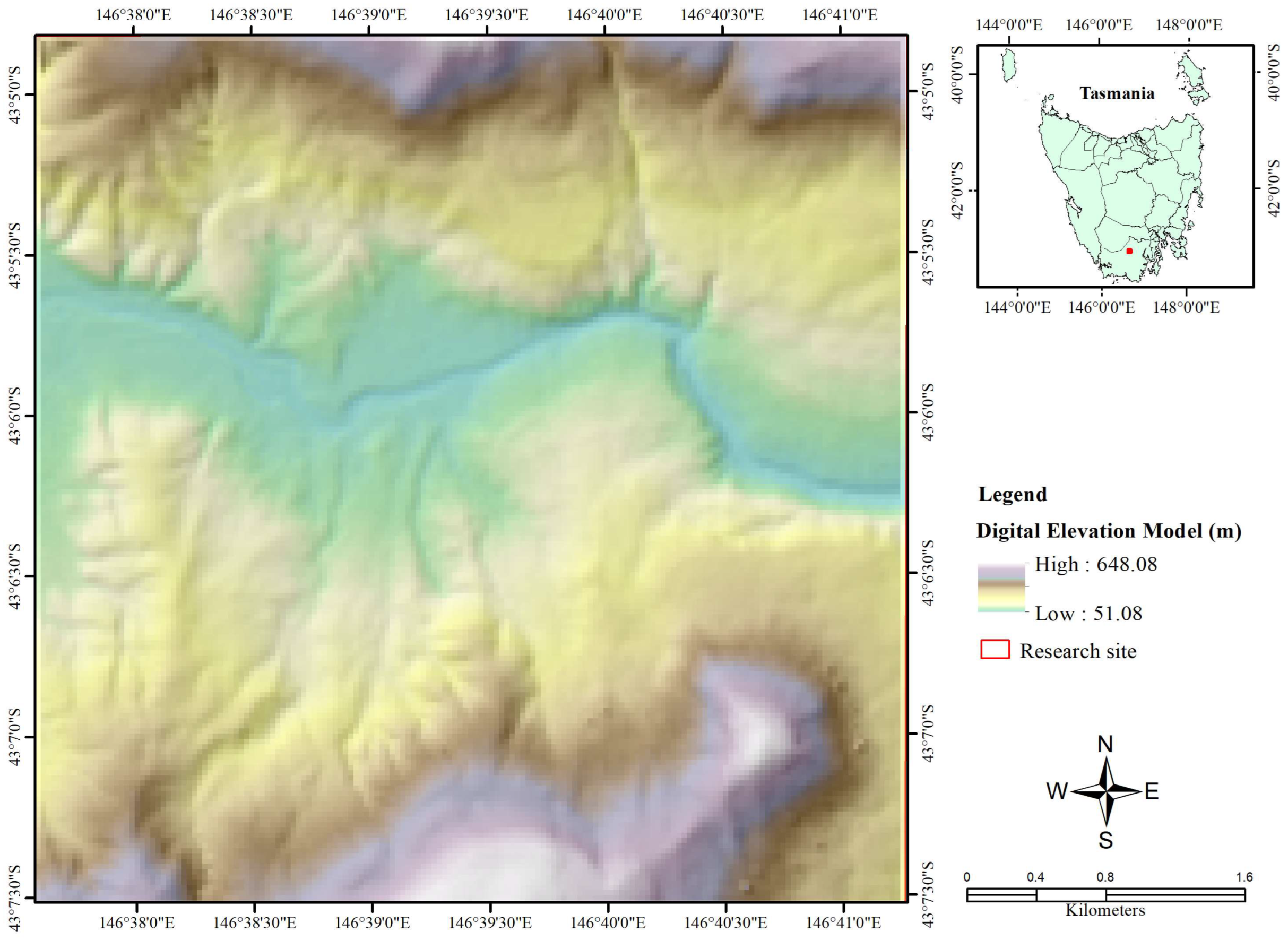
Figure 2.
Workflow for assessing the robustness of multispectral satellite imagery with LiDAR topographic attributes and a geology data layer to predict vertical structure in a wet eucalypt forest.
Figure 2.
Workflow for assessing the robustness of multispectral satellite imagery with LiDAR topographic attributes and a geology data layer to predict vertical structure in a wet eucalypt forest.
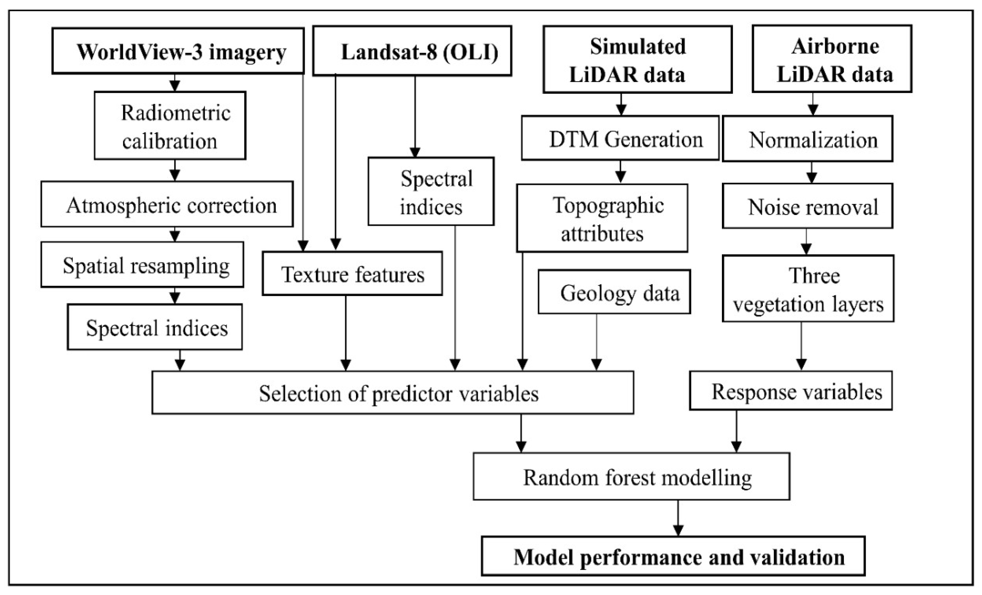
Figure 3.
Predicted mean R2 from the 13 schemes of predictor variables derived from the 30 m Landsat-8 (OLI) satellite imagery and the simulated operational LiDAR data. Here, a scheme means a group of predictor variables used for RF modelling. Spectral bands = B, spectral indices = I, texture features = T, topographic attributes = A, geology vector data = G.
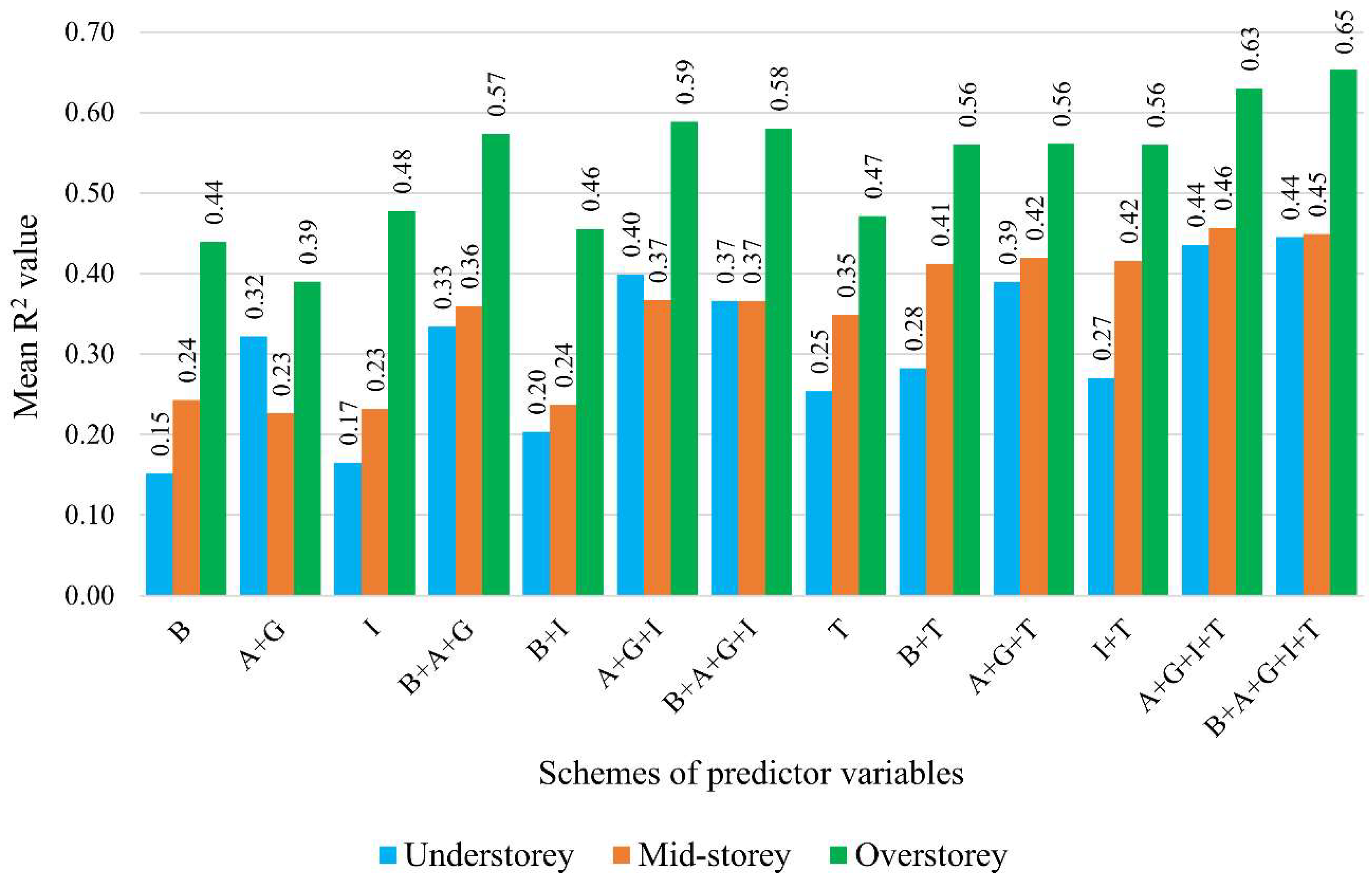
Figure 4.
Predicted mean R2 values from the 13 schemes of predictor variables derived from the 30 m resampled WorldView-3 satellite imagery and the simulated operational LiDAR data.
Figure 4.
Predicted mean R2 values from the 13 schemes of predictor variables derived from the 30 m resampled WorldView-3 satellite imagery and the simulated operational LiDAR data.
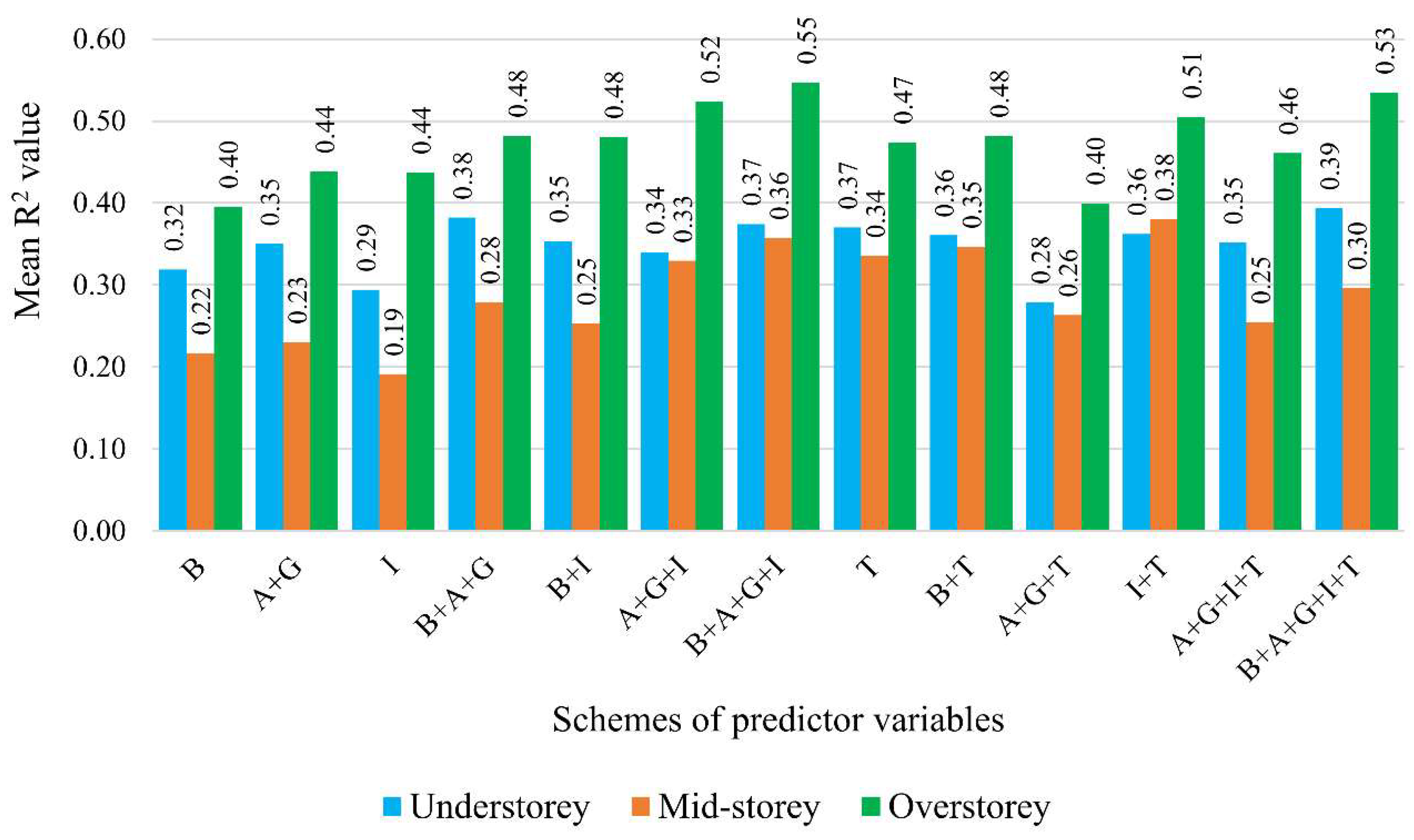
Figure 5.
Predicted mean R2 from the 13 schemes of predictor variables derived from the 7.5 m simulated VNIR and original SWIR bands of WorldView-3 satellite imagery and the simulated operational LiDAR data.
Figure 5.
Predicted mean R2 from the 13 schemes of predictor variables derived from the 7.5 m simulated VNIR and original SWIR bands of WorldView-3 satellite imagery and the simulated operational LiDAR data.
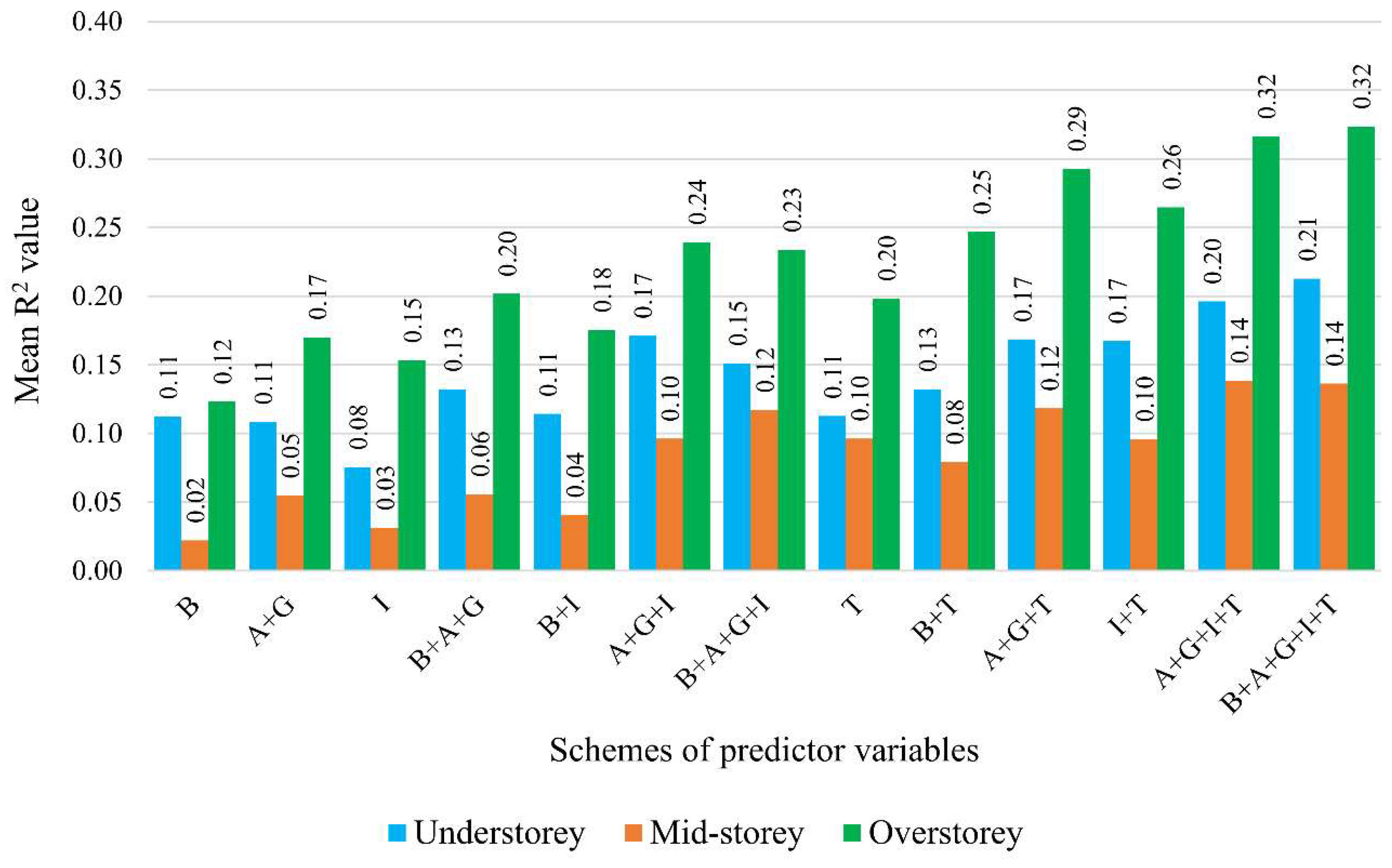
Figure 6.
Predicted mean R2 from the 13 schemes of predictor variables derived from the 1.6 m VNIR bands of WorldView-3 satellite imagery and the simulated operational LiDAR data.
Figure 6.
Predicted mean R2 from the 13 schemes of predictor variables derived from the 1.6 m VNIR bands of WorldView-3 satellite imagery and the simulated operational LiDAR data.
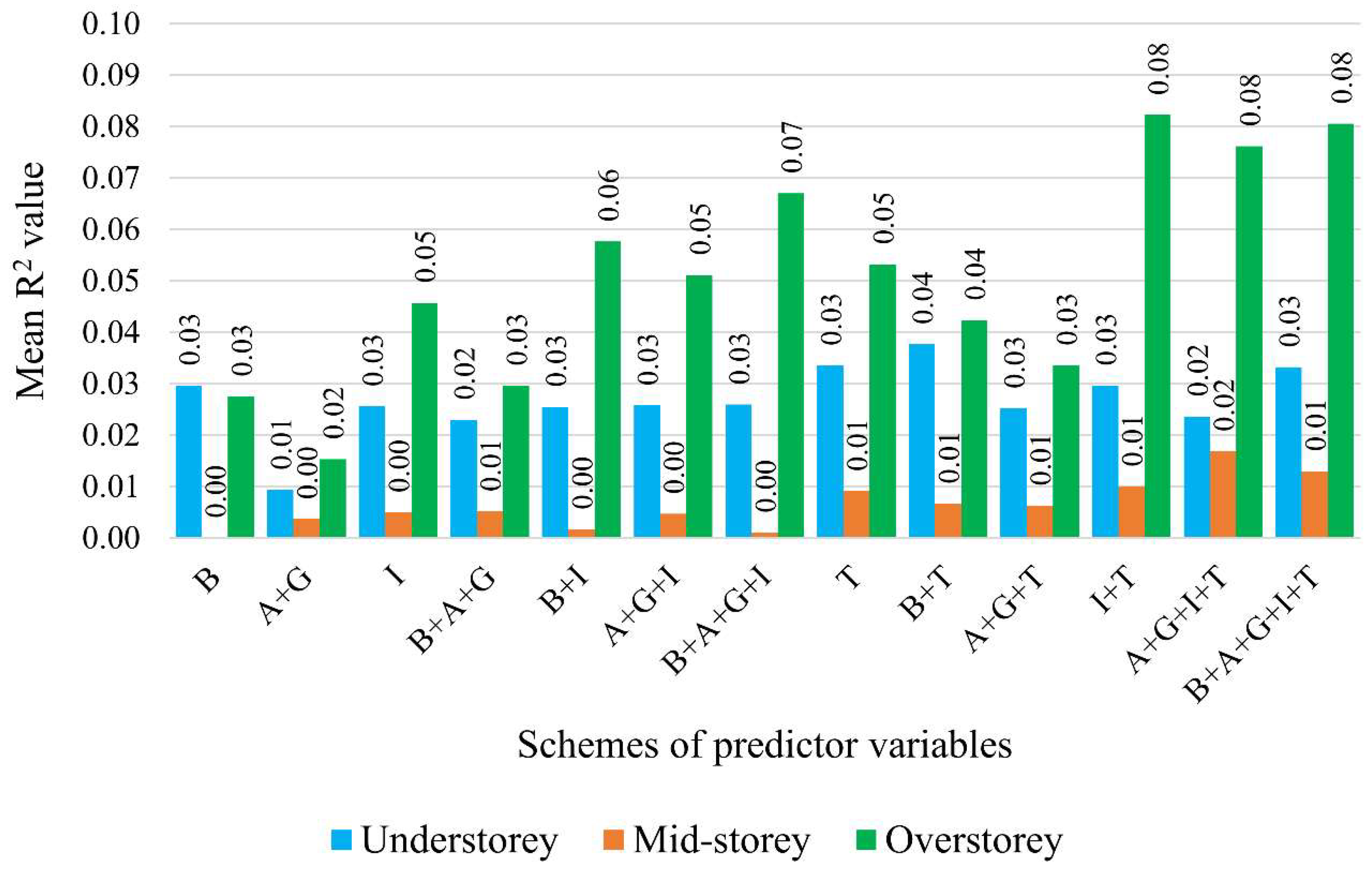
Figure 7.
Accuracy differences (validated-predicted) of thirteen schemes using the 30 m Landsat-8 satellite imagery with topographic attributes and geology data. Positive values indicate more and negative values less than the validated accuracies.
Figure 7.
Accuracy differences (validated-predicted) of thirteen schemes using the 30 m Landsat-8 satellite imagery with topographic attributes and geology data. Positive values indicate more and negative values less than the validated accuracies.
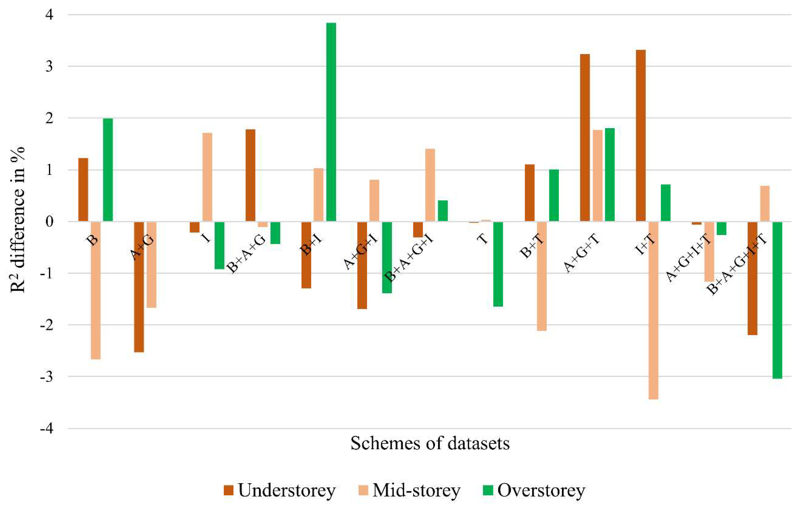
Figure 8.
Accuracy differences (validated-predicted) of thirteen schemes using the 30 m WorldView-3 imagery with topographic attributes and geology data.
Figure 8.
Accuracy differences (validated-predicted) of thirteen schemes using the 30 m WorldView-3 imagery with topographic attributes and geology data.
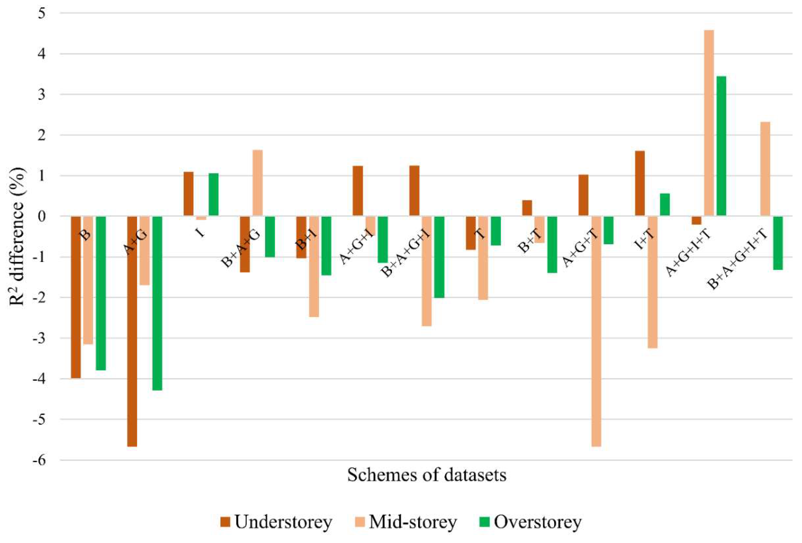
Figure 9.
Importance of the top 20 predictor variables using Landsat-8 (OLI) bands combined with topographic attributes, spectral indices, and texture features.
Figure 9.
Importance of the top 20 predictor variables using Landsat-8 (OLI) bands combined with topographic attributes, spectral indices, and texture features.
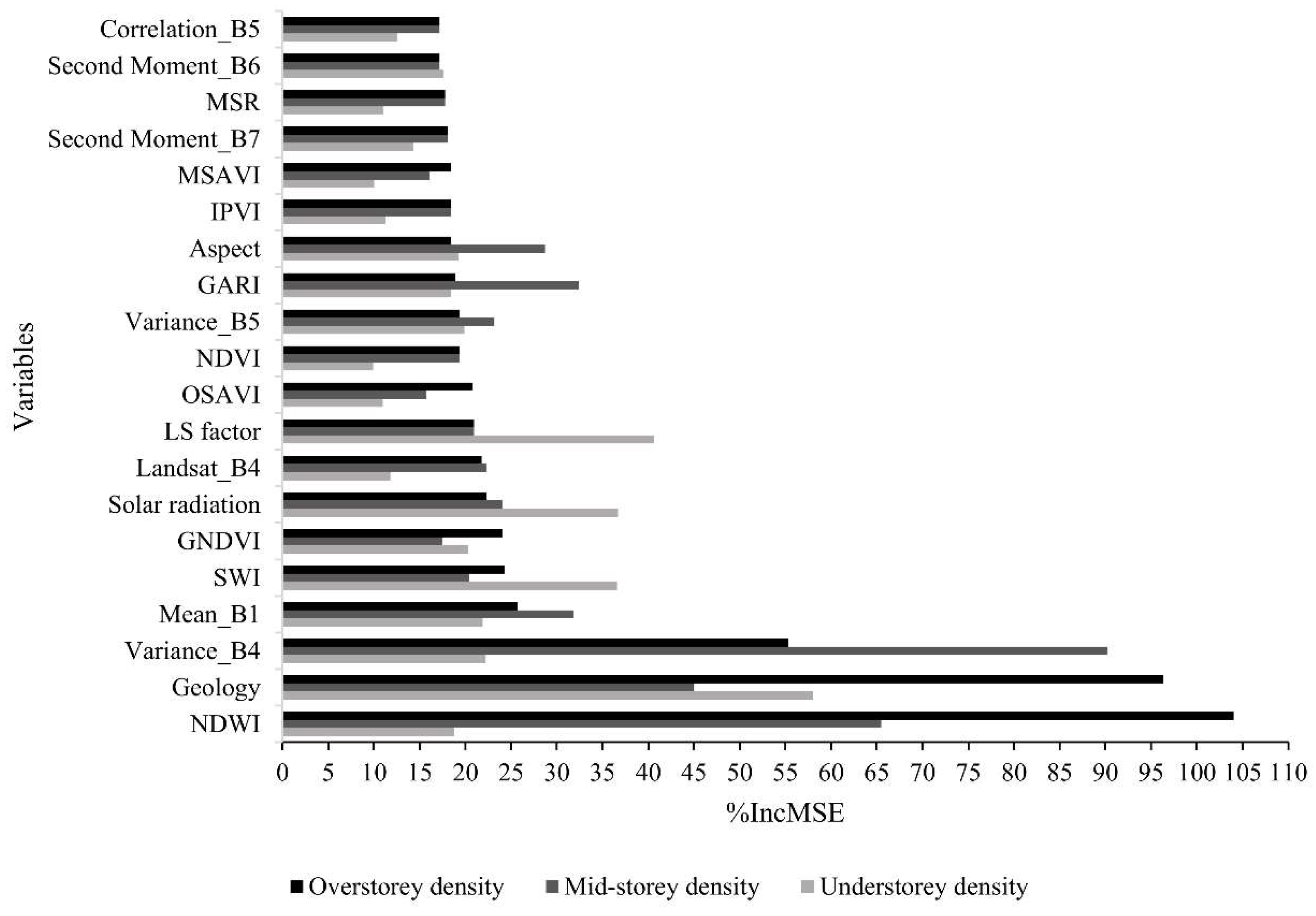
Figure 10.
Importance of the top 20 predictor variables using the resampled bands of WorldView 30 m combined with topographic attributes, spectral indices, and texture features.
Figure 10.
Importance of the top 20 predictor variables using the resampled bands of WorldView 30 m combined with topographic attributes, spectral indices, and texture features.
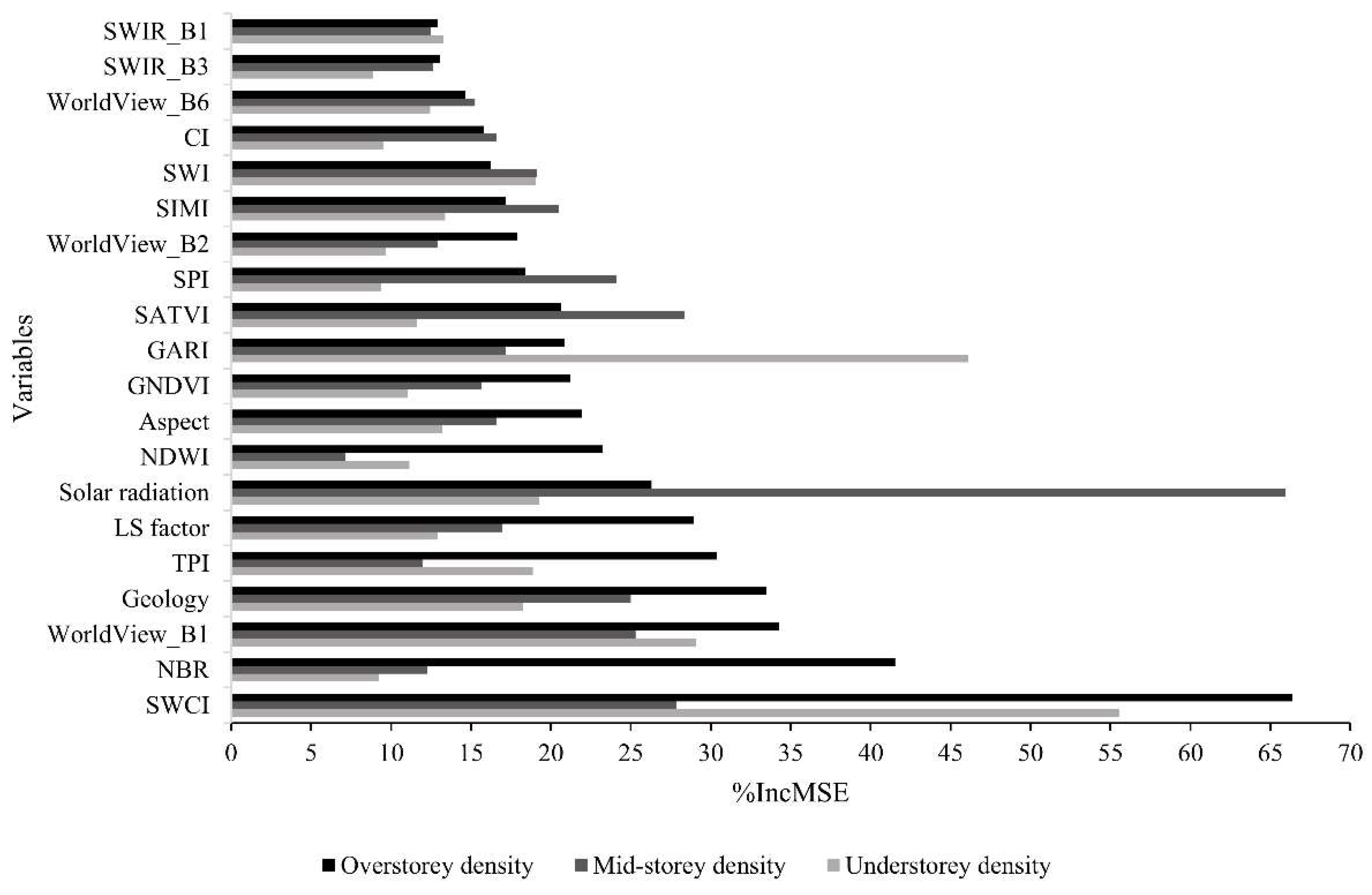
Table 1.
Specifications of multispectral remote sensing datasets.
| Specification item | WorldView-3 Imagery | Landsat-8 Imagery |
|---|---|---|
| Date of acquisition | 2015-10-05 | 2014-10-21 |
| Spatial resolution | 1.60 m (VNIR bands) 7.50 m (SWIR bands) |
30 m (VNIR and SWIR bands) |
| Sun azimuth | 42.400 | 48.800454560 |
| Sun Elevation | 43.700 | 48.182282610 |
| Product Type Level | "Standard" LV2A | OLI_TIRS_L1TP |
| Bands (In Nanometres) |
Coastal = 427.40 Blue = 481.90 Green = 547.10 Yellow = 604.30 Red = 660.10 Red Edge = 722.70 NIR1= 824.00 NIR2 = 913.60 SWIR1 = 1209.10 SWIR2= 1571.60 SWIR3= 1661.10 SWIR4= 1729.50 SWIR5= 2163.70 SWIR6= 2202.20 SWIR7= 2259.30 SWIR8= 2329.20 |
Coastal = 442.96 Blue = 482.04 Green = 561.41 Red = 654.59 NIR = 864.67 SWIR 1 = 1608.86 SWIR 2 = 2200.73 |
Table 2.
Absolute radiometric calibration adjustment factors and irradiance values for WorldView-3 as of 1/29/2016 Kuester [64].
Table 2.
Absolute radiometric calibration adjustment factors and irradiance values for WorldView-3 as of 1/29/2016 Kuester [64].
| Band | Gain value | Offset value | Solar irradiance value (W-M-2 −μm-1) [66] |
|---|---|---|---|
| Coastal | 0.863 | -7.154 | 1757.89 |
| Blue | 0.905 | -4.189 | 2004.61 |
| Green | 0.907 | -3.287 | 1830.18 |
| Yellow | 0.938 | -1.816 | 1712.07 |
| Red | 0.945 | -1.350 | 1535.33 |
| Red-Edge | 0.980 | -2.617 | 1348.08 |
| NIR 1 | 0.982 | -3.752 | 1055.94 |
| NIR 2 | 0.954 | -1.507 | 858.77 |
| SWIR 1 | 1.160 | -4.479 | 479.019 |
| SWIR 2 | 1.184 | -2.248 | 263.797 |
| SWIR 3 | 1.173 | -1.806 | 225.283 |
| SWIR 4 | 1.187 | -1.507 | 197.552 |
| SWIR 5 | 1.286 | -0.622 | 90.4178 |
| SWIR 6 | 1.336 | -0.605 | 85.0642 |
| SWIR 7 | 1.340 | -0.423 | 76.9507 |
| SWIR 8 | 1.392 | -0.302 | 68.0988 |
Disclaimer/Publisher’s Note: The statements, opinions and data contained in all publications are solely those of the individual author(s) and contributor(s) and not of MDPI and/or the editor(s). MDPI and/or the editor(s) disclaim responsibility for any injury to people or property resulting from any ideas, methods, instructions or products referred to in the content. |
© 2025 by the authors. Licensee MDPI, Basel, Switzerland. This article is an open access article distributed under the terms and conditions of the Creative Commons Attribution (CC BY) license (http://creativecommons.org/licenses/by/4.0/).
Copyright: This open access article is published under a Creative Commons CC BY 4.0 license, which permit the free download, distribution, and reuse, provided that the author and preprint are cited in any reuse.


