
Submitted:
05 June 2024
Posted:
07 June 2024
You are already at the latest version
Abstract
Accurately assessing forest structure and maintaining up-to-date information about forest structure is crucial for various forest planning efforts, including the development of reliable forest plans and assessments of the sustainable management of natural resources. Field measurements traditionally applied to acquire forest inventory information (e.g., basal area, tree volume, and aboveground biomass) are labor-intensive and time-consuming. To address this limitation, remote sensing tech-nology has been widely applied in modeling efforts to help estimate forest inventory information. Among various remotely sensed data, LiDAR can potentially help describe forest structure. This study was conducted to estimate and map forest inventory information across the Talladega Na-tional Forest by employing ALS-derived data and aerial photography. The quality of predictive models was evaluated to determine whether additional remotely sensed data can help improve forest structure estimates. Additionally, the quality of general predictive models was compared to that of species-group models. This study confirms that quality level 2 LiDAR data was sufficient for developing adequate predictive models (R2adj. ranging between 0.71 and 0.82) when compared to the predictive models based on LiDAR and aerial imagery. Additionally, this study suggests that species-group predictive models were of higher quality than general predictive models. Lastly, landscape-level maps were created from the predictive models, and these may be helpful to plan-ners, forest managers, and landowners in their management efforts.
Keywords:
Aerial imagery
; airborne laser scanning
; forest inventory
; LiDAR
; Mixed pine hardwood forest
1. Introduction
The ability to adequately characterize and assess forest structure with a high level of accuracy is not only important for the development of a reliable forest plan but is also informative for assessments that demonstrate the sustainable management of natural resources [1,2]. Within this context, an understanding of forest conditions, particularly growing stock (tree and stand volume), aboveground biomass, and basal area, is crucial for planners, forest managers, and landowners. These attributes directly influence the potential revenue and the potential habitat a forest can provide and facilitate opportunities for addressing other management objectives [2,3]. Furthermore, a regularly updated forest inventory is essential for monitoring the spatiotemporal dynamics of forest ecosystems over the length of a planning horizon. For example, an estimate of aboveground biomass can provide insights into the capacity of a forest to sequester carbon, which is considered a critical factor in addressing climate change. This issue may become more important in the future as the forestry sector faces increasing pressure to assess the ability and rate of forests to sequester carbon [4,5,6,7]. Additionally, estimates of biomass can provide valuable information for assessing forest health related to the outbreak of Southern pine beetle [8] and for assessing fire risk associated with fuel management [9].
Traditionally, an estimate of a forest inventory has heavily relied on labor-intensive and time-consuming field measurements. Timely field measurements may be limited in spatiotemporal coverage, may include sampling error, and may not be representative of large forested areas [10]. While measuring the diameter at breast height (dbh) of trees, identifying the tree species, and counting trees within a sample unit (e.g., plot or prism point) are relatively straightforward methods, estimating the height of each tree may require more effort and include more uncertainty [11], especially in natural, mountainous forest landscapes [7]. Endeavors meant to obtain a sufficient number of well-distributed sampling plots that properly represent an entire forest area remain challenging due to limited resources and accessibility. To account for these limitations, traditional field measurements have been complemented by products derived from remote sensing systems, which may help address spatial and temporal challenges in developing a forest inventory [3,12]. This approach is sometimes referred to as an enhanced forest inventory [13,14]. Within this framework various remote sensing systems have been demonstrated to provide relatively accurate and cost-effective forest information including the development of forest metrics [2,3,10,15,16] and greenhouse gas inventories [17].
Data acquired from Light Detection and Ranging (LiDAR) devices can assist in the development of forestry information. Unlike other remote sensing processes that only provide two-dimensional information, LiDAR can characterize three-dimensional forest structure to a certain extent based on the point density of the LiDAR data [5,16,18]. LiDAR can help with deriving height estimates of an object through the time interval between the emission of a pulse of energy by the LiDAR sensor and the moment that the reflected signal has been returned to the device [19]. This type of active remote sensing technology has advanced significantly in the last ten years, resulting in a diverse range of LiDAR systems that can be installed in satellites, mounted on airplanes and unmanned aerial vehicles (UAVs), or used as hand-held devices. Each type of system has advantages and disadvantages. For instance, one advantage of using satellite-based laser scanning platforms such as NASA’s Global Ecosystem Dynamics Investigation (GEDI) and Ice Cloud and Land Elevation Satellite 2 (ICESat-2) is that they can provide multi-temporal data for the entire Earth. For instance, Potapov et al. [20] was able to create a global canopy height model using GEDI data along with Landsat imagery. Additionally, Dubayah et al. [21] presented the estimate of mean biomass densities for every country covered by GEDI with 1 km resolution.
Terrestrial-based LiDAR platforms can be categorized as either static or mobile. Terrestrial laser scanners (TLS) capture point clouds by looking upward from ground level, so they are advantageous in capturing details of forest structure from under the canopy. Especially, static TLS platforms (consisting of a sensor, a tripod, and a GNSS receiver) produce the highest-quality point clouds among LiDAR systems [5,22]. Appropriately employed TLS can facilitate visualization of tree branches and leaves; therefore, these systems have enormous potential for assisting in the development of new allometric biomass and wood quality relationships [23]. Arseniou et al. [24], for example, was able to estimate woody aboveground biomass for urban and rural settings using a TLS platform to identify various tree parts other than the main stem. Nevertheless, TLS platforms have several limitations when employed for forest inventory and operational forest management purposes. One, an occlusion effect, is caused by features hidden or obstructed behind larger diameter trees within the point cloud data, and it poses a challenge when a fixed-position, single-scan approach is used [25]. In addition, the weight and size of a TLS platform can make the effort of moving between field measurement plots challenging. These limitations, along with the cost of the platform, may influence opinions of whether TLS is a practical alternative for collecting forest inventory [26,27].
Mobile laser scanning (MLS) platforms, which is mobile TLS platforms, capture point clouds by looking horizontally from a height near ground level, where they are held, making them advantageous for capturing details of forest structure from a perspective very similar to human-collected field measurements. MLS platforms can collect information while a person traverses sampling plots with the instrument held in the person's hand or carried in a backpack. Moreover, the development of point clouds that are georeferenced to a local coordinate reference system, using Simultaneous Localization and Mapping (SLAM) algorithms, reduces the need for GNSS. While numerous researchers have illustrated the applicability of MLS for diverse forest inventory tasks [7,10,28,29], these studies often focus on MLS data collected at the plot-level. Among them, Vatandaşlar et al. [7] estimated several forest attributes (tree counts, dominant height, basal area, dbh, stand volume, and relative density) within plots located in a near-natural forest landscape. Employing a handheld MLS platform, Vatandaşlar et al. [7] mapped every stem within each field measurement plot and estimated these attributes with RMSEs ranging between 4.5% and 16.4%. However, as with TLS platforms, the number of sampling plots employed will likely influence the accuracy of forest or stand estimates [23]. As with any measurement system, the accuracy of forest attribute estimations can be positively correlated with the number of plots measured [30]. For instance, the diverse forests of the Talladega Division of the Talladega National Forest in the southeastern US cover almost 93,694 ha [31], and thus the number of TLS or MLS plots needed to describe forest character relatively accurately may be substantial. Therefore, an alternative solution needs to be sought to effectively and efficiently characterize the forest inventory of large, diverse areas such as this.
In this context, airborne laser scanning (ALS) systems have been considered a suitable choice for helping to describe the forest character of broad areas. Notably, the ALS data acquisition process is not constrained by the accessibility restrictions related to TLS including static and mobile platforms [5]. The versatility of an ALS system allows the collection of information across diverse temporal and spatial scales [32]. Recent advancements in sensor technologies have further encouraged the adoption of ALS systems, allowing the development of regularly updated and increasingly dense point clouds. For instance, a LiDAR-based forest inventory effort conducted in Ontario two decades ago resulted in a point cloud dataset with about 0.5 points per m2, yet today the development of a point cloud dataset above 40 points per m2 can be obtained [33].
While forest attributes such as tree heights and canopy coverage can be directly estimated from ALS LiDAR data, other forest characteristics such as aboveground biomass, growing stock (tree volume), and basal area can be inferenced from LiDAR-derived metrics [5]. The development of these estimates relies on modeling methods, which can range in complexity from regression to random forest models and other machine learning techniques [34]. Distinct models for estimating characteristics of different forest types (conifer, broadleaved, and mixed) might also be developed, rather than a general model that is applicable to an entire forested area. Further research in this domain is necessary, with a specific emphasis on investigating the nature by which additional spectral data can enhance the predictive capability of LiDAR point clouds. Additionally, as mathematical techniques and remotely sensed data evolve, the most effective combination of methods and data sources needs to be assessed.
A map of forest characteristics for an extensive forest area is an ideal outcome of remote sensing methods, yet this outcome is complicated by two underlying factors: the multitude of potential independent variables that can be derived from remotely sensed data, and the potential correlation amongst these which can induce a multicollinearity problem [35,36]. Furthermore, a large number of independent variables within predictive models can challenge the application of these models for developing broad scale GIS databases. Consequently, the selection of independent variables during the model development process is important. Tibshirani [37] suggested a method for developing linear models that estimate forest conditions, while enhancing prediction accuracy by reducing the number of independent variables. Adhikari et al. [35] recommended the use of ALASSO, as it effectively eliminated highly correlated independent variables from prediction models.
The main goal of this study is to develop models to estimate forest conditions across a broad area from information provided by ALS and aerial imagery. This research effort seeks to: (i) evaluate the quality of predictive models developed using the ALASSO method, (ii) evaluate whether additional remotely sensed data (multispectral aerial imagery) can enhance the quality of predictive models that rely on LiDAR point cloud data, and (iii) determine the suitability of general versus species group-specific models for characterizing mixed coniferous and deciduous forests located in the southern United States. We use the Talladega Division of the Talladega National Forest as our case study area because it represents typical characteristics of natural, pine-dominated forests of southeastern USA. National forest managers do not have comprehensive inventories of the extent under management limiting global decision space for at risk resources be it wildland fire, forest health, endangered species habitat condition to help assess where management is needed or has achieved desired future conditions. Therefore models, maps, and other outcomes derived from predictive models that are based on LiDAR (and other) data may provide forest managers, researchers, and policymakers with valuable insight to monitor and manage forests throughout the southeastern USA.
2. Materials and Methods
2.1. Study Area
This study was conducted within the boundaries of the Talladega Division of the Talladega National Forest, located in northwestern Alabama, USA. This 93,694-ha part of the national forest lies within the Piedmont and Ridge and Valley ecoregions [31]. The climate in this area generally consists of mild winters and hot summers, which are characteristic of a humid, subtropical climate. Elevation of the lands in the Talladega Division varies between approximately 160 m to 735 m above sea level, and annual precipitation is around 1260 mm. Historically, the forests in the study area have been composed of coniferous species such as longleaf pine (Pinus palustris Mill.), shortleaf pine (P. echinata Mill.), and loblolly pine (P. taeda), particularly in the uplands and on south-facing slopes. Deciduous tree species are often found in the riparian areas and on north-facing slopes. Oak (Quercus spp.), hickory (Carya spp.), maple (Acer spp.), and yellow-poplar (Liriodendron tulipifera) are among the more prevalent deciduous tree species in the study area.
2.2. Data Collection
2.2.1. Field Data Collection
A set of 254 fixed area, circular plots (402.6 m2 with a 11.32 m radius) were measured by U.S. Forest Service crews between February and April 2022. These plots were pseudo-randomly located within the operable (upland) lands of the study area. An equal number of plots were measured within eight forest structure classes, defined by canopy density and tree height. Plot locations were limited to the interior (rather than edges) of management units (stands), and only one plot per management unit was allowed. Plot centers were mapped using a Trimble R1 GNSS receiver (Trimble, Colorado, USA). The field data collection procedure followed methods described in Laes et al. [38]. Within each plot, several characteristics of each live tree (height, dbh, tree species, tree crown status (dominant and co-dominant), azimuth, and distance from the plot center) were recorded. A dbh larger than 7.6 cm (3 inches) and a height greater than 0.6 m (2 feet) represented the minimum sizes of measured live trees.
2.2.2. Remote Data Collection
True color and near-infrared images of five counties that cover the study area were captured during the leaf-off season between 2020 (December) and 2021 (February). These images were used to create county mosaic orthophotographs with a spatial resolution of 0.3 m. The county mosaic images were acquired from the U.S. Department of Agriculture National Agricultural Imagery Program (NAIP) [39]. The ALS data was collected using a Leica Terrain Mapper. Within the study area, the ALS data contained 13.92 billion points. The average point density achieved was 9.7 points per m2 and ranged from 3.5 points per m2 to 20.3 points per m2. The horizontal and vertical accuracy of the LiDAR data (0.71 m and 0.051 m, respectively) was estimated using 441 survey points spread across the State of Alabama. These characteristics satisfy the requirements for at least topographic quality level 2 (QL2) [40].
2.3. Data Processing
2.3.1. Field Data Processing
From the field measurement plots we estimated a variety of forest attributes related to tree heights (minimum, maximum, dominant, and mean merchantable height), tree dbh (minimum, maximum, quadratic mean of dbh, arithmetic mean of dbh, and coefficient of variation of dbh), canopy conditions (mean crown ratio), volume per unit area, and aboveground biomass per unit area. Among these, we focus on basal area (m2 ha-1), tree volume (m3 ha-1), and aboveground biomass (Mg ha-1) as dependent variables for the modeling effort. Basal area was estimated based on dbh, and tree volume and aboveground biomass were estimated using species-specific allometric equations from the U.S. Forest Service (National Biomass Estimator Library (NBEL) and National Volume Estimator Library (NVEL) which are Excel Add-ins developed by the Forest Management Service Center, U.S. Forest Service). Additionally, we classified sampling plots by the dominant tree species present, based on the total basal area for a species in a given plot exceeding 70% of the total basal area. As a result, there were only 14 oak dominant sampling plots and 149 pine dominated sampling plots (i.e., pine plots). All other plots indicated no dominance towards a specific tree species (i.e., mixed plots). Accordingly, we separately developed models based on two datasets (a) using all plots (n=254), and (b) pine plots (n=149).
2.3.2. Remote Data Processing
From NAIP imagery we created vegetation indices (i.e., greenness, Normalized Difference Vegetation Index (NDVI), and Enhanced Vegetation Index (EVI)) for the study area using ArcGIS Pro (Esri, Redlands, CA, USA). A total of 24 vegetation indices were developed and utilized as NAIP-derived independent variables (Table 1).
Due to the large file size of the raw LiDAR point cloud data, processing could not be completed with a desktop personal computer. Thus, the LiDAR point cloud data was processed using RStudio (R version 2023.06.1 Build 524) and the University of Georgia’s Georgia Advanced Computing Resource Center’s Sapelo2 Linux (64-bit CentOS 7.9) high-performance computing cluster. To reduce the processing time, parallel computing was used with 21 cores utilized simultaneously with a total of 900 GB RAM. The raw LiDAR data were first utilized to create a digital terrain model using only those points in the point cloud classified as bare ground. In creating the digital terrain model, selecting an appropriate algorithm and spatial resolution are important because it directly affects the result of estimated vegetation metrics [18]. Because of this, the spatial resolution was chosen based on point spacing and the number of points in the point cloud as suggested by McCullagh [41] and Hengl [42]. The triangular irregular network algorithm, a vector terrain model using Delaunay triangles, was applied to create a 1 m spatial resolution digital terrain model. With the digital terrain model representing the ground, we then generated a normalized LiDAR point cloud including only the above ground points. The first returns in the normalized point cloud were then used to create a canopy height model. Noise, resulting from points within the point cloud with negative values or values greater than 95% of the height, were removed to increase the quality of regression models. LiDAR-derived metrics were then calculated from point clouds that were clipped using the boundary of each sampling plot using R package (‘lidR’, version 4.0.3). We extracted 56 LiDAR-derived metrics from the normalized LiDAR point clouds for 254 of sampling plots. Among LiDAR-derived metrics, we excluded certain metrics with absolute values (such as maximum height and intensity, mean intensity, area, point counts, and total intensity), assuming that the LiDAR sensor was not calibrated for light conditions before data collection, and to avoid developing a model with variables that were return-density dependent. Therefore, a total of 74 independent variables were developed including 50 LiDAR-derived metrics (Table 2) and 24 NAIP-derived metrics which are used as independent variables in the modeling effort.
2.4. Modeling
We created 12 models to estimate three forest attributes (basal area, volume, aboveground biomass) with two different sets of field measurement sampling plots (all plots, pine plots) and two types of data sources (LiDAR only, LiDAR + NAIP). Depending on which field measurement sampling plots were employed, two sets of regression models were created: General models and pine models. Due to the high number of independent variables derived from LiDAR and NAIP data sources, inter-correlation between independent variables and the complexity of models was inevitable [3]. To reduce the complexity of models and to avoid multicollinearity issues, we applied the ALASSO regression. As ALASSO regression is a regularization technique, it addresses multicollinearity issues by shrinking regression coefficients to zero based on the lambda value which minimizes the sum of the squared differences between predicted values and observed values. The best lambda was obtained by applying 10-fold cross-validation. Prior to applying ALASSO regression, the normality of data was assessed using the Box-Cox method. Given the results of the Box-Cox method, a natural logarithmic transformation was applied to the dependent variables, improving the linearity of the data, the homogeneity of residual variances, and the normality of residuals. Additionally, potential outliers were investigated using Cook’s distance and studentized residuals. The observed outliers without leverage were eliminated. The best models were selected based on various parameters including the R2adj., the number of independent variables, root mean square of error (RMSE), Collin Mallow’s Cp, Akaike’s information criteria (AIC), and Bayesian Information Criterion (BIC). The models were back transformed by exponentiating the dependent variable and were applied to estimate the forest attributes for the broader study area. Lastly, 10-fold cross-validation was applied to evaluate the quality of the models. While the modeling procedures were conducted using RStudio (R version 2023.06.1 Build 524) on a desktop computer, broad scale estimation maps were processed using the Sapelo2 Linux based high-performance computing cluster.
3. Results
3.1. Field-Based Forest Inventory
The average basal area, tree volume and aboveground biomass of the 254 field measurement sampling plots was about 23.4 m2 ha-1, 180.9 m3 ha-1, and 40.1 Mg ha-1, respectively (Table 3). For the pine dominated field measurement plots, the average basal area, tree volume, and aboveground biomass were about 22.3 m2 ha-1, 169.0 m3 ha-1, and 34.6 Mg ha-1, respectively. The range of values for the sampling plots was large since the plots were meant to be representative of all forest conditions in the study area, from early successional to mature forest stages.
3.2. Regression Models
3.2.1. Estimation of Forest Attributes Based on General Models
In nearly every case, the LiDAR + NAIP regression models included a larger number of independent variables than the LiDAR-only models. In the basal area model based on LiDAR + NAIP, five vegetation indices (GMIN, NDVIMIN, NDVIMEDIAN, EVIMAX, and EVIPCT90) were additionally selected instead of the zq30 variable (30th percentile height distribution from the ground) found in the basal area model based on LiDAR-only (Table 4). The R2adj. values for the basal area models were 0.72 (cross-validation: 0.69) for LiDAR + NAIP and 0.71 (cross-validation: 0.71) LiDAR-only, while RMSE values were 5.6 m2 ha-1 (cross-validation: 5.90 m2 ha-1) for LiDAR + NAIP and 5.7 m2 ha-1 (cross-validation: 5.91 m2 ha-1) LiDAR-only (Table 5). Other quality metrics except AIC also indicated that the model based on LiDAR + NAIP performed slightly better than the model based on LiDAR-only. The predicted basal area tended to be underestimated as its basal area increased regardless of data sources (Figure 2).
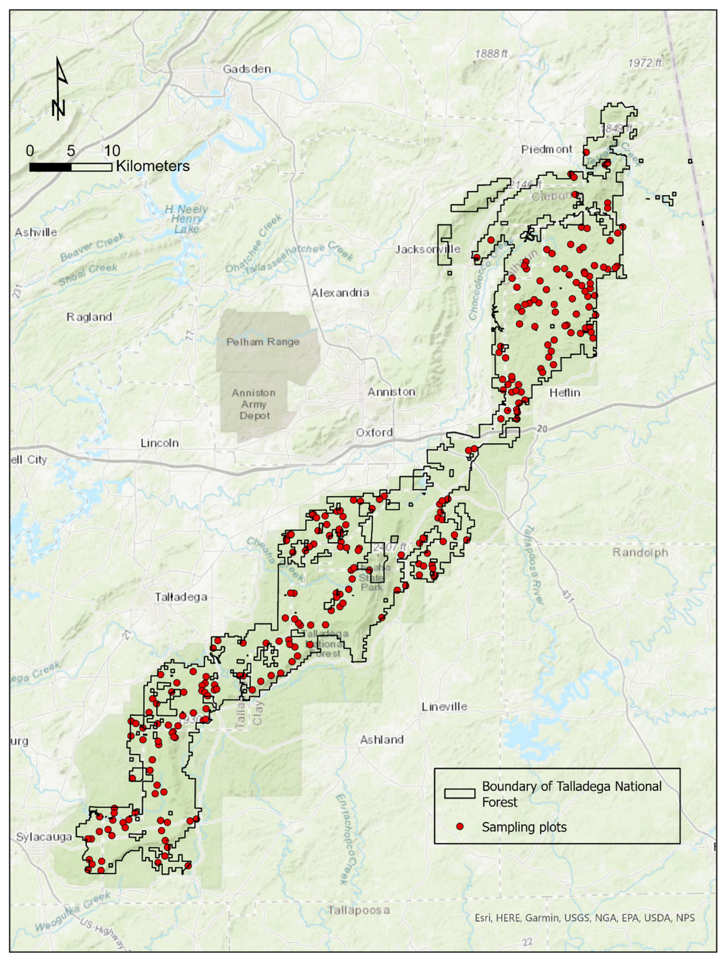
Figure 1.
Locations of the field measurement sample plots within the study area (Sources: Esri. “World Topographic Map” [basemap]. January 31, 2024).
Figure 1.
Locations of the field measurement sample plots within the study area (Sources: Esri. “World Topographic Map” [basemap]. January 31, 2024).
In the volume models, a higher R2adj. value (0.77) was observed (Table 5). Although the overall quality metrics for LiDAR + NAIP and LiDAR-only models represented a similar level of performance, the increment in the number of independent variables in LiDAR + NAIP models was noticeable as it increased from 12 to 21 (Table 4). Specifically, eight independent variables derived from NAIP imagery were selected. Additionally, a LiDAR-derived metric, zpcum5 (cumulative percentile of return in the 5th layer), was also selected as an independent variable in LiDAR + NAIP model yet was not used in the LiDAR-only model. As observed in the basal area models, the difference between observed volume and estimated volume tended to increase with higher volume regardless of data sources (Figure 2).
The aboveground biomass models had R2adj. values that were 0.73 and 0.72 (cross-validation: 0.64 and 0.65) for LiDAR + NAIP and LiDAR-only models, respectively (Table 5). Similar to the basal area models, the LiDAR + NAIP model yielded slightly more accurate RMSE values than the LiDAR-only model (LiDAR + NAIP model: 11.7 Mg ha-1 (cross-validation:13.05 Mg ha-1); LiDAR-only model: 11.8 Mg ha-1(cross-validation:13.09 Mg ha-1)). Nevertheless, the difference between aboveground biomass models depending on data sources was slight. Five vegetation indices were added into the LiDAR + NAIP model as independent variables (Table 4). Both aboveground biomass models underestimated biomass for the sample plots having higher aboveground biomass, suggesting estimation errors increase as forest stands mature (Figure 2).
The average R2adj. and average R2 values of 10-fold cross-validation results ranged from 0.64 to 0.73 and from 0.68 to 0.75, respectively (Table 6). The difference between statistics of cross-validation and developed models were generally smaller in LiDAR based models compared to the LiDAR + NAIP models. Regarding the selection of independent variables, several metrics were commonly selected regardless of data source, including: pzabove2, zq95, zpcum6, isd, iskew, ikurt, ipcumzq90 and p2th (all from LiDAR data); and GMIN, NDVIMIN and EVIPCT90 (all from NAIP data) (Table 7).
3.2.2. Estimation of Forest Attributes Based on Pine Models
The R2adj. and RMSE values of basal area models were 0.81 and 0.80 (R2adj. of cross-validation: 0.79 and 0.75), and 4.8 m2 ha-1 and 5.1 m2 ha-1 (RMSE of cross-validation: 5.21 m2 ha-1 and 5.71 m2 ha-1) for LiDAR + NAIP and LiDAR, respectively (Table 8). Noticeable improvements in quality metrics of LiDAR + NAIP models were not observed by supplementing independent variables using NAIP derived metrics. Interestingly, there was no increase in the number of independent variables, but three NAIP derived metrics (NDVIMIN, NDVIMEDIAN, and EVIPCT90) were selected instead of LiDAR derived metrics (zpcum6, ipcumzq30, ipcumzq90) (Table 4). The visual interpretation of the scatter plots showed that basal area tended to be underestimated as basal area values increased regardless of the data sources (Figure 3). Similar trends in scatter plots were also observed in general models, but the distribution of points was closer to the 1:1 line.
Regarding the volume models, R2adj. values of 0.84 (cross-validation: 0.78) for LiDAR + NAIP and 0.82 (cross-validation: 0.79) for LiDAR-only models achieved (Table 8). The RMSE values ranged from 37.9 m3 ha-1 to 43.5 m3 ha-1 (cross-validation: from 47.44 m3 ha-1 to 48.94 m3 ha-1) which were lower than comparable values of the general regression models. However, AIC and BIC of general volume regression models were lower than those of the pine volume regression models. The increment in number of independent variables in LiDAR + NAIP models was notable as it increased from 11 to 30 in volume models. Specifically, eight independent variables derived from NAIP images were added to the LiDAR + NAIP regression model (Table 4). Additionally, 12 independent variables derived from LiDAR point clouds were added on the LiDAR + NAIP regression model.
The aboveground biomass models had R2adj. values of 0.83 (cross-validation: 0.80) for LiDAR + NAIP and 0.82 (cross-validation: 0.78) for LiDAR-only models (Table 8). The RMSE values of aboveground biomass models were 7.9 Mg ha-1 and 8.9 Mg ha-1 (cross-validation: 9.4 Mg ha-1 and 10.2 Mg ha-1) for LiDAR + NAIP and LiDAR-only, respectively. Regarding AIC and BIC values, our results indicated that the quality of LiDAR-only models was better than the LiDAR + NAIP models. The number of independent variables also noticeably increased in LiDAR + NAIP models (LiDAR + NAIP: 34; LiDAR-only: 10). Ten NAIP derived metrics were selected in addition to 16 LiDAR derived metrics in LiDAR + NAIP model (Table 4). Similar to the general regression models, both models (LiDAR + NAIP and LiDAR-only) underestimated aboveground biomass for the sample plots having higher biomass estimates, suggesting estimation errors increased as stands mature (Figure 3).
The average R2adj. values of 10-fold cross-validation results of pine models ranged from 0.75 to 0.80 regardless of forest attributes and data sources (Table 9). The average R2 values of 10-fold cross-validation results for the pine model ranged from 0.78 to 0.84. Developed models based on LiDAR + NAIP for basal area and aboveground biomass were more robust than developed models based on LiDAR-only. Otherwise, the developed model based on LiDAR + NAIP for the volume less robust that developed models based on LiDAR-only. Similar to the general models, there were some LiDAR and NAIP derived metrics which were commonly selected as independent variables in every pine model regardless of forest attributes: pzabove2, zq5, zq95, zpcum5, iskew, ikurt, and p2th (all from LiDAR data); and NDVIMIN, EVIPCT90, and NDVIMEDIAN (all from NAIP data) (Table 7).
4. Discussion
Estimating forest attributes such as basal area, volume, and aboveground biomass and updating this information regularly are critical activities for forest management and planning efforts. This study attempted to improve the performance of forest attribute estimations for large areas using LiDAR point clouds and high-resolution, multispectral remotely sensed data. We investigated the effect of different combinations of remotely sensed data (LiDAR-only or LiDAR + NAIP) on the quality of regression models. Also, we evaluated the quality of regression models depending on the classification of sampling plots according to species mixture. To avoid the overfitting issue resulting from multicollinearity between independent variables, the ALASSO method was employed during the modeling process as this method performance was suggested by earlier studies [35,43]. Eventually, a total of 12 models were developed for three forest attributes (basal area, volume, aboveground biomass) based on the species mixture (all species and pine), as well as data source (LiDAR-only, LiDAR + NAIP). When the general models are applied to the case study landscape, broad scale maps of these resource conditions can be visualized (Figure 4, Figure 5 and Figure 6).
The R2adj. values of developed models ranged from 0.71 to 0.84 which were comparable to other ALS study results [3,34,44]. While many researchers have developed regression models for estimating forest attributes over relatively small forested areas [10,15,19,34,36], there have been few attempts to work in large areas such as U.S. National Forests. For instance, Leboeuf et al. [44] mapped a merchantable wood volume of very large area (440,000 km2) using airborne LiDAR. However, this study had a few limitations, including significant temporal differences between the field measurements (2003-2018) and LiDAR data (2011-2020) collection periods, limited spatial resolution, and poor representativeness of sampling plots. In our study, however, field and remote sensing datasets were collected during a relatively similar period of time (2020-2022). The distribution of sample plots is also important in developing robust regression models for forest attribute estimation. To enhance the quality of regression models, we used a stratified pseudo-random sampling design by classifying the entire operable study area with consideration of recent management activities to improve the balance and representation of the heterogeneity of the forest in the sampling design. Additionally, we surveyed all tree species (both merchantable and non-merchantable > 7.62 cm in dbh) within sampling plots to enhance the accuracy of regression models, as suggested by Brown et al. [45].
The R2adj. values and R2 values of pine models were higher than those of the general models regardless of forest attributes. The overall quality metrics also indicated pine models were higher compared to the general models. Bouvier et al. [3] also confirmed that separate models may result in higher accuracy when compared to general models. Regarding forest attributes, the highest R2adj. values were observed in tree volume models and the lowest R2adj. values were observed in basal area models regardless of data sources and sampling plots (all plots or pine plots). This trend has also been observed in other studies using ALS systems [3,34,46,47]. Sumnall et al. [48] suggested that basal area models have relatively lower R2 values than models estimating tree height and biomass. This is likely because, unlike tree height, dbh cannot be directly measured with ALS systems. Dbh is used to estimate basal area, yet dbh and tree height are often needed to estimate volume and aboveground biomass [3], therefore it may be logical to observe that the basal area estimation models would underperform the volume and biomass models.
There have been many attempts recently to enhance the performance of regression models for estimating forest conditions. They generally involve the development of LiDAR metrics [3,49], and perhaps supplementary remotely sensed data [34,45]. In this study, the vegetation indices derived from NAIP imagery were included as supplemental data. As the additional NAIP imagery had higher spatial resolution (0.3 m), we expected the vegetation indices might improve the quality of regression models to a considerable extent. However, it was observed that the addition of NAIP-derived vegetation metrics was not very influential in improving the quality of prediction models. Although LiDAR-only derived models had slightly larger RMSE values and slightly lower R2 values compared to the LiDAR + NAIP derived models, the increase in the number of independent variables with the addition of NAIP metrics led us to conclude that LiDAR-only models were more appropriate for broad-scale mapping efforts.
Of the 74 metrics derived from LiDAR and NAIP data sources, 45 were selected as independent variables in at least one regression model. Further, five LiDAR-based metrics and two NAIP-based metrics were selected for every regression model (Table 7). These were, specifically, the LiDAR-based metrics pzabove2, zq95, iskew, ikurt, and p2th, and the NAIP-based metrics NDVIMIN and EVIPCT90. LiDAR-based metrics pzabove2 and p2th metrics help eliminate the effect of understory vegetation that is not measured in a typical forest inventory survey. The LiDAR-based metric zq95 is widely used to represent forest canopy height. In addition to height related LiDAR metrics, intensity related metrics, such as iskew and ikurt, were also crucial in developing regression models as they provide information related to stand density. The inclusion of NAIP-based NDVIMIN and EVIPCT90 can be explained by the concentration of active chlorophyll in pine tree crowns. Ozkan et al. [34] also confirmed that metrics such as these may be significantly correlated with forest attributes.
Although inclusion of NAIP-based metrics improved the accuracy of the regression models we developed, we suggest that LiDAR-derived metrics may be sufficient for developing robust regression models used for operational forest management purposes. Interestingly, the general trend in the spatial pattern of basal area, volume, and aboveground biomass is due to the high correlation among these forest attributes (Figure 4, Figure 5 and Figure 6). Since aboveground biomass of a forest is typically a derivation of growing stock, volume estimates often rely on dbh measurements, and as basal area is directly related to dbh, these relationships may help in developing simple ratios between forest conditions without the need for additional, elaborate regression models. While this may potentially decrease the reliability of some of the outcomes, the practicality of the overall effort may be worth investigating further.
5. Conclusions
The objective of this study was to estimate and map key forest attributes across a wide area of interest, utilizing ALS data and aerial imagery. To achieve this objective, we employed the ALASSO modeling method, relying on 254 field measurement plots from a national forest in Alabama (USA), a mostly natural ecosystem composed of coniferous and deciduous tree species. One of the main conclusions drawn from our findings was that the LiDAR data collected by the ALS system with topographic quality level QL2 character seems to be a sufficient input for the development of regression models that can estimate basal area, volume, and aboveground biomass at accuracy levels that are acceptable for operational forest inventories. A second conclusion was that the added value of using optical data (aerial imagery) and associated vegetation indices as inputs for the development of regression models for estimating basal area, volume, and aboveground biomass was negligible, considering the increased model complexity and extra time required to process and analyze the additional model inputs. A third conclusion was that the models exclusively developed for areas dominated by pine species seem to outperform (with respect to the coefficient of determination from cross-validation) general models that were developed for all tree species within the study area. While we affirmed these conclusions for natural, pine-dominated forests in the study area, further research was needed to assess the scalability of the results to other forest ecosystems of the southern USA.
Supplementary Materials
The following supporting information can be downloaded at the website of this paper posted on Preprints.org, Figure S1: Estimated basal area for the entire study area based on general model (Sources: Esri. “World Topographic Map” [basemap]. January 31, 2024).; Figure S2: Estimated tree volume for the entire study area based on general model (Sources: Esri. “World Topographic Map” [basemap]. January 31, 2024).; Figure S3: Estimated aboveground biomass for the entire study area based on general model (Sources: Esri. “World Topographic Map” [basemap]. January 31, 2024).
Author Contributions
Conceptualization, T.L., C.V., and P.B.; methodology, A.P. and T.L.; validation, T.L. and C.V.; formal analysis, T.L.; data curation, T.L. and J.S.; writing—original draft preparation, T.L. and C.V.; writing—review and editing, T.L., C.V., B.P., K.M., J.S., A.P.; visualization, T.L. and K.M.; supervision, P.B.; project administration, P.B.; funding acquisition, P.B. All authors have read and agreed to the published version of the manuscript.
Funding
This work was supported in part by Talladega Division LiDAR Project 2022-Part 2, US Forest Service Agreement No. 22-CS-11080100-232, and in part by Promoting Economic Resilience and Sustainability of the Eastern US Forests (PERSEUS), U.S. Department of Agriculture Award No. 2023-68012-38992.
Data Availability Statement
We encourage all authors of articles published in MDPI journals to share their research data. In this section, please provide details regarding where data supporting reported results can be found, including links to publicly archived datasets analyzed or generated during the study. Where no new data was created, or where data is unavailable due to privacy or ethical restrictions, a statement is still required. Suggested Data Availability Statements are available in section “MDPI Research Data Policies” at https://www.mdpi.com/ethics.
Conflicts of Interest
The authors declare no conflicts of interest.
References
- Bettinger, P.; Boston, K.; Siry, J.P.; Grebner, D.L. Forest management and planning. Academic Press, London. 2017.
- Jarron, L.R.; Coops, N.C.; MacKenzie, W.H.; Tompalski, P.; Dykstra, P. Detection of sub-canopy forest structure using airborne LiDAR. Remote Sens. Environ. 2020, 244, 111770. [CrossRef]
- Bouvier, M.; Durrieu, S.; Fournier, R.A.; Renaud, J.P. Generalizing predictive models of forest inventory attributes using an area-based approach with airborne LiDAR data. Remote Sens. Environ. 2015, 156, 322-334. [CrossRef]
- Chen, Y.; Kershaw, J.A.; Hsu, Y.H.; Yang, T.R. Carbon estimation using sampling to correct LiDAR-assisted enhanced forest inventory estimates. Forestry Chron. 2020, 96 (1), 9-19. [CrossRef]
- Du, L.; Pang, Y.; Wang, Q.; Huang, C.; Bai, Y.; Chen, D.; Lu, W.; Kong, D. A LiDAR biomass index-based approach for tree-and plot-level biomass mapping over forest farms using 3D point clouds. Remote Sens. Environ. 2023, 290, 113543. [CrossRef]
- Tian, L.; Wu, X.; Tao, Y.; Li, M.; Qian, C.; Liao, L.; Fu, W. Review of remote sensing-based methods for forest aboveground biomass estimation: Progress, challenges, and prospects. Forests. 2023, 14 (6), 1086. [CrossRef]
- Vatandaşlar, C.; Seki, M.; Zeybek, M. Assessing the potential of mobile laser scanning for stand-level forest inventories in near-natural forests. Forestry. 2023, 96 (4), 448-464. [CrossRef]
- Nowak, J.T.; Meeker, J.R.; Coyle, D.R.; Steiner, C.A.; Brownie, C. Southern pine beetle infestations in relation to forest stand conditions, previous thinning, and prescribed burning: Evaluation of the southern pine beetle prevention program. J. Forest. 2015, 113(5), 454-462. [CrossRef]
- Ager, A.A.; Vaillant, N.M.; Finney, M.A. Integrating fire behavior models and geospatial analysis for wildland fire risk assessment and fuel management planning. J. Combust. 2011. [CrossRef]
- Adhikari, A.; Peduzzi, A.; Montes, C.R.; Osborne, N.; Mishra, D.R. Assessment of understory vegetation in a plantation forest of the southeastern United States using terrestrial laser scanning. Ecol. Inform. 2023, 77, 102254. [CrossRef]
- Seki, M.; Sakici, O.E. Ecoregion-based height-diameter models for Crimean pine. J. For. Res. 2022, 27, 36-44. [CrossRef]
- García, M.; Riaño, D.; Chuvieco, E.; Danson, F.M. Estimating biomass carbon stocks for a Mediterranean forest in central Spain using LiDAR height and intensity data. Remote Sens. Environ. 2010, 114 (4), 816-830. [CrossRef]
- White, J.C.; Coops, N.C.; Wulder, M.A.; Vastaranta, M.; Hilker, T.; Tompalski, P. Remote sensing technologies for enhancing forest inventories: A review. Can. J. Remote Sens. 2016, 42 (5): 619-641. [CrossRef]
- White, J.C.; Tompalski, P.; Vastaranta, M.; Wulder, M.A.; Saarinen, N.; Stepper, C.; Coops, N.C. A model development and application guide for generating an enhanced forest inventory using airborne laser scanning data and an area based approach. Canadian Wood Fibre Centre: Victoria, BC, Canada. Information Report FI-X-018. 2017, 38. ISBN 978-0-660-09738-1.
- Ferraz, A.; Saatchi, S.; Mallet, C.; Meyer, V. Lidar detection of individual tree size in tropical forests. Remote Sens. Environ. 2016, 183, 318-333. [CrossRef]
- Lim, K.; Treitz, P.; Wulder, M.A.; St-Onge, B.; Flood, M.; LiDAR remote sensing of forest structure. Prog. Phys. Geog. 2003, 27 (1), 88-106. https://doi.org/10.1191/0309133303pp360.
- McRoberts, R.E.; Næsset, E.; Sannier, C.; Stehman, S.V.; Tomppo, E.O. Remote sensing support for the gain-loss approach for greenhouse gas inventories. Remote Sens. 2020, 12 (11), 1891. [CrossRef]
- Bater, C.W.; Coops, N.C. Evaluating error associated with Lidar-derived DEM interpolation. Comput. Geosci. 2009, 35, 289-300. [CrossRef]
- García-Gutiérrez, J.; Martínez-Álvarez, F.; Troncoso, A.; Riquelme, J.C. A comparison of machine learning regression techniques for LiDAR-derived estimation of forest variables. Neurocomputing. 2015, 167, 24-31. [CrossRef]
- Potapov, P.; Li, X.; Hernandez-Serna, A.; Tyukavina, A.; Hansen, M.C.; Kommareddy, A.; Pickens, A.; Turubanova, S.; Tang, H.; Silva, C.E.; Armston, J.; Dubayah, R.; Blair, J.B.; Hofton, M. Mapping global forest canopy height through integration of GEDI and Landsat data. Remote Sens. Environ. 2021, 253, 112165. https:// doi. org/10. 3390/ rs120 30505.
- Dubayah, R.; Armston, J.; Healey, S.P.; Bruening, J.M.; Patterson, P.L.; Kellner, J.R.; Duncanson, L.; Saarela, S.; Ståhl, G.; Yang, Z.; Tang, H. GEDI launches a new era of biomass inference from space. Environ. Res. Lett. 2022, 17(9), 095001. [CrossRef]
- Liang, X.; Kankare, V.; Hyyppä, J.; Wang, Y.; Kukko, A.; Haggrén, H.; Yu, X.; Kaartinen, H.; Jaakkola, A.; Guan, F.; Holopainen M.; Vastaranta, M. Terrestrial laser scanning in forest inventories. ISPRS J. Photogramm. 2016, 115, 63-77. [CrossRef]
- Liang, X.; Kukko, A.; Balenović, I.; Saarinen, N.; Junttila, S.; Kankare, V.; Holopainen, M.; Mokroš, M.; Surový, P.; Kaartinen, H.; Jurjević, L.; Honkavaara, E.; Näsi, R.; Liu, J.; Hollaus, M.; Tian, J.; Yu, X.; Pan, J.; Cai, S.; Virtanen, J.P.; Wang, Y.; Hyyppä, J.; Close-range remote sensing of forests: The state of the art, challenges, and opportunities for systems and data acquisitions. IEEE Geosci. Remote Sens. Mag. 2022, 10 (3), 32-71. [CrossRef]
- Arseniou, G.; MacFarlane, D.W.; Calders, K.; Baker, M. Accuracy differences in aboveground woody biomass estimation with terrestrial laser scanning for trees in urban and rural forests and different leaf conditions. Trees. 2023, 37, 761-779. [CrossRef]
- Mathes, T.; Seidel, D.; Häberle, K.H.; Pretzsch, H.; Annighöfer, P.; What are we missing? Occlusion in laser scanning point clouds and its impact on the detection of single-tree morphologies and stand structural variables. Remote Sens. 2023, 15 (2), 450. [CrossRef]
- Chen, S.; Liu, H.; Feng, Z.; Shen, C.; Chen, P. Applicability of personal laser scanning in forestry inventory. PLoS One. 2019, 14 (2), e0211392. [CrossRef]
- Ryding, J.; Williams, E.; Smith, M.; Eichhorn, M. Assessing handheld mobile laser scanners for forest surveys. Remote Sens. 2015, 7 (1), 1095–1111. [CrossRef]
- Gollob, C.; Ritter, T.; Nothdurft, A. Forest inventory with long range and high-speed personal laser scanning (PLS) and simultaneous localization and mapping (SLAM) technology. Remote Sens. 2020, 12 (9), 1509. [CrossRef]
- Mokroš, M.; Mikita T.; Singh A.; Tomastík J.; Chudá J.; Wezyk P.; Kuželka, K.; Surový, P.; Klimánek, M.; Zięba-Kulawik, K.; Bobrowski, R.; Liang, X. Novel low-cost mobile mapping systems for forest inventories as terrestrial laser scanning alternatives. Int. J. Appl. Earth Obs. Geoinf. 2021, 104, 102512. [CrossRef]
- Li, C.; Yu, Z.; Dai, H.; Zhou X.; Zhou M. Effect of sample size on the estimation of forest inventory attributes using airborne LiDAR data in large-scale subtropical areas. Ann. Forest Sci. 2023, 80, 40. [CrossRef]
- Stober, J.; Merry, K.; Bettinger, P. Analysis of fire frequency on the Talladega National Forest, USA, 1998–2018. Int. J. Wildland Fire. 2020, 29 (10), 919–925. [CrossRef]
- Yao, H.; Qin, R.; Chen, X. Unmanned aerial vehicle for remote sensing applications-A review. Remote Sens. 2019, 11 (12), 1443. [CrossRef]
- Penner, M.; Woods, M.; Bilyk, A. Assessing site productivity via remote sensing—age-independent site index estimation in even-aged forests. Forests. 2023, 14 (8), 1541. [CrossRef]
- Ozkan, U.Y.; Demirel, T.; Ozdemir, I.; Saglam, S.; Mert, A. Predicting forest stand attributes using the integration of airborne laser scanning and Worldview-3 data in a mixed forest in Turkey. Adv. Space Res. 2022, 69 (2), 1146-1158. [CrossRef]
- Adhikari, A.; Montes, C.R.; Peduzzi, A. A comparison of modeling methods for predicting forest attributes using Lidar metrics. Remote Sens. 2023, 15 (5), 1284. [CrossRef]
- Chen, X.; Xie, D.; Zhang, Z.; Sharma, R.P.; Chen, Q.; Liu, Q.; Fu, L. Compatible biomass model with measurement error using airborne LiDAR data. Remote Sens. 2023, 15 (14), 3546. [CrossRef]
- Tibshirani, R. Regression shrinkage and selection via the lasso. J. R. Stat. Soc. Ser. B (Methodol.). 1996, 73 (1), 267–288.
- Laes, D.; Reutebuch, S.E.; McGaughey, R.J.; Mitchell, B. Guidelines to estimate forest inventory parameters from lidar and field plot data. 2011, Available at: https://fsapps.nwcg.gov/gtac/CourseDownloads/Reimbursables/FY21/Lidar_Material/GTAC_Guidelines%20to%20estimate%20forest%20inventory%20parameters%20from%20lidar%20and%20field%20plot%20data.pdf.
- U.S. Department of Agriculture. National Agriculture Imagery Program (NAIP). U.S. Department of Agriculture, Washington, D.C. 2023. https://naip-usdaonline.hub.arcgis.com/ (Accessed May 2, 2024).
- U.S. Geologic Survey. Topographic data quality levels (QLs). U.S. Geologic Survey, Reston, VA. 2024. https://www.usgs.gov/3d-elevation-program/topographic-data-quality-levels-qls (Accessed April 22, 2024).
- McCullagh, M.J. Terrain and surface modelling systems: Theory and practice. Photogramm. Rec. 1988, 12 (72), 747-779. [CrossRef]
- Hengl, T. Finding the right pixel size. Comput. Geosci. 2006, 32 (9), 1283-1298. [CrossRef]
- Henn, K.A.; Peduzzi, A. Biomass estimation of urban forests using LiDAR and high-resolution aerial imagery in Athens–Clarke County, GA. Forests. 2023, 14 (5), 1064. [CrossRef]
- Leboeuf, A.; Riopel, M.; Munger, D.; Fradette, M.S.; Bégin, J. Modeling merchantable wood volume using Airborne LiDAR metrics and historical forest inventory plots at a provincial scale. Forests. 2022, 13 (7), 985. [CrossRef]
- Brown, S.; Narine, L.L.; Gilbert, J. Using airborne lidar, multispectral imagery, and field inventory data to estimate basal area, volume, and aboveground biomass in heterogeneous mixed species forests: A case study in southern Alabama. Remote Sens. 2022, 14 (11), 2708. [CrossRef]
- Hawbaker, T.J.; Keuler, N.S.; Lesak, A.A.; Gobakken, T.; Contrucci, K.; Radeloff, V.C. Improved estimates of forest vegetation structure and biomass with a LiDAR-optimized sampling design. J. Geophys. Res. Biogeo. 2009, 114, G00E04. [CrossRef]
- Silva, C.A.; Hudak, A.T.; Vierling, L.A.; Loudermilk, E.L.; O’Brien, J.J.; Hiers, J.K.; Jack, S.B.; Gonzalez-Benecke, C.; Lee, H.; Falkowski, M.J.; Khosravipour, A. Imputation of individual longleaf pine (Pinus palustris Mill.) tree attributes from field and LiDAR data. Can. J. Remote Sens. 2016, 42 (5), 554-573. ttps://doi.org/10.1080/07038992.2016.1196582.
- Sumnall, M.J.; Hill, R.A.; Hinsley, S.A. Towards forest condition assessment: evaluating small-footprint full-waveform airborne laser scanning data for deriving forest structural and compositional metrics. Remote Sens. 2022, 14 (20), 5081. [CrossRef]
- Yan, W.Y.; Van Ewijk, K.; Treitz, P.; Shaker, A. Effects of radiometric correction on cover type and spatial resolution for modeling plot level forest attributes using multispectral airborne LiDAR data. ISPRS J. Photogramm. 2020, 169, 152-165. [CrossRef]
Figure 2.
The observed forest attributes versus the predicted forest attributes of the general models (n=254). (LiDAR+NAIP: A, C, E; LiDAR: B, D, F).
Figure 2.
The observed forest attributes versus the predicted forest attributes of the general models (n=254). (LiDAR+NAIP: A, C, E; LiDAR: B, D, F).
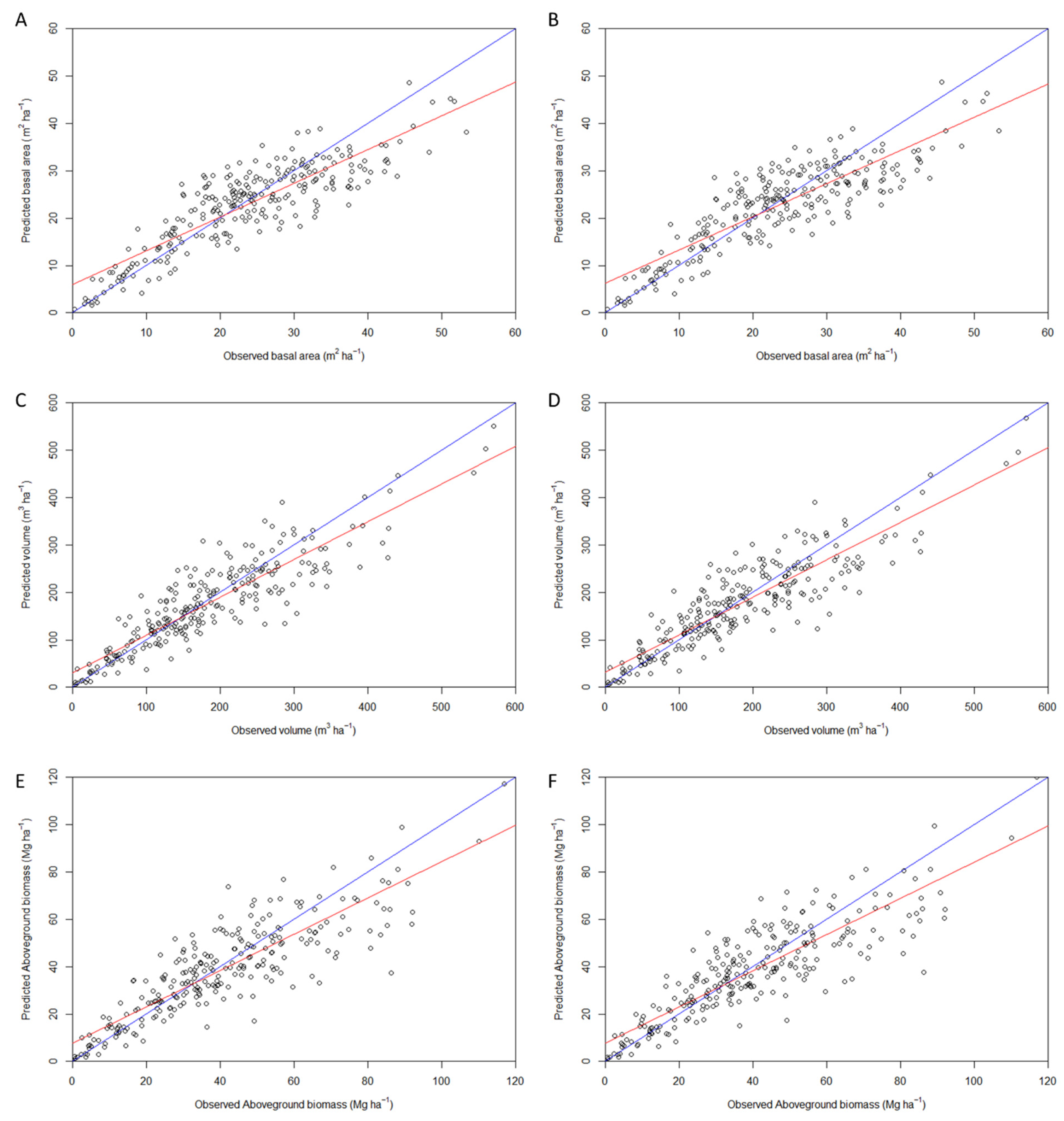
Figure 3.
The observed forest attributes versus the predicted forest attributes of the pine models (n=149). (LiDAR+NAIP: A, C, E; LiDAR: B, D, F).
Figure 3.
The observed forest attributes versus the predicted forest attributes of the pine models (n=149). (LiDAR+NAIP: A, C, E; LiDAR: B, D, F).
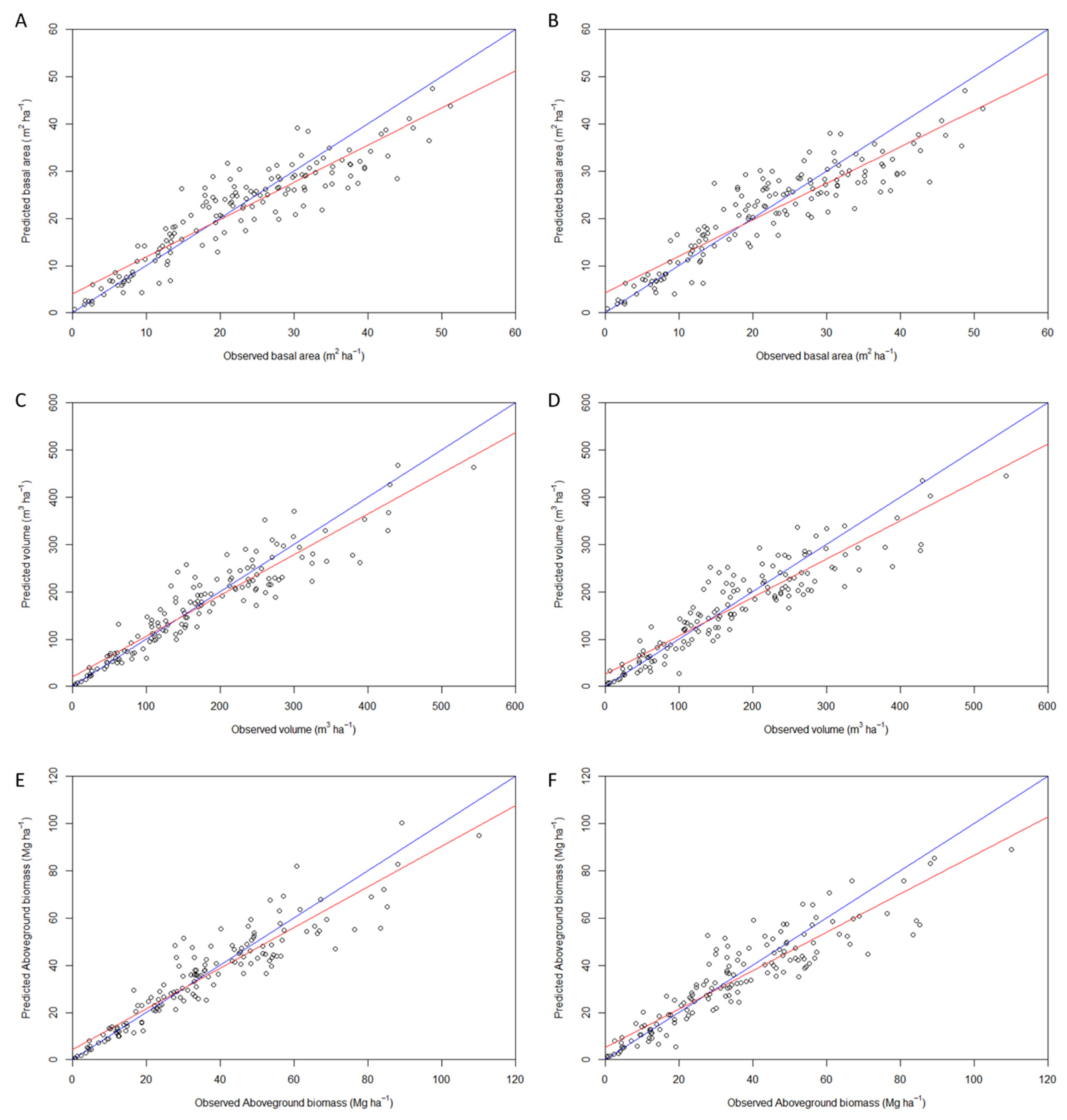
Figure 4.
Estimated basal area for a portion of the study area based on general model (Sources: Esri. “World Topographic Map” [basemap]. January 31, 2024).
Figure 4.
Estimated basal area for a portion of the study area based on general model (Sources: Esri. “World Topographic Map” [basemap]. January 31, 2024).
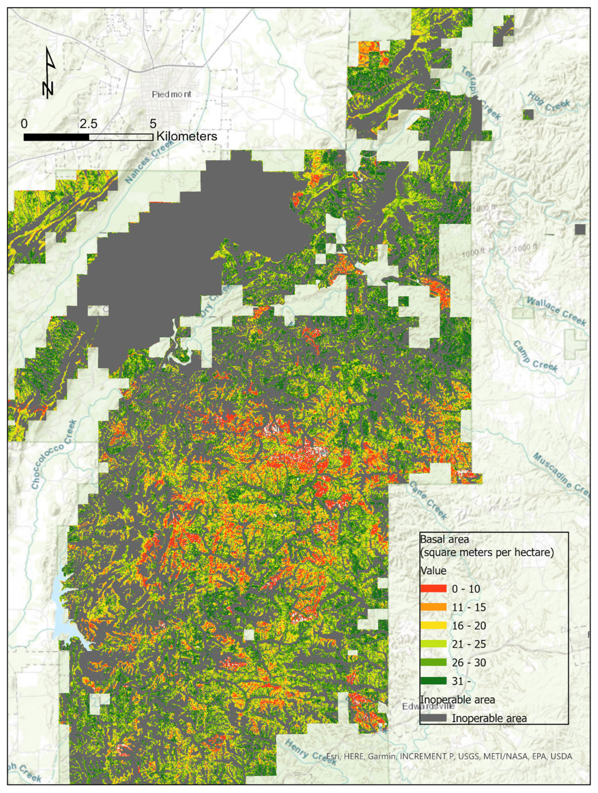
Figure 5.
Estimated volume per hectare for a portion of the study based on general model (Sources: Esri. “World Topographic Map” [basemap]. January 31, 2024).
Figure 5.
Estimated volume per hectare for a portion of the study based on general model (Sources: Esri. “World Topographic Map” [basemap]. January 31, 2024).
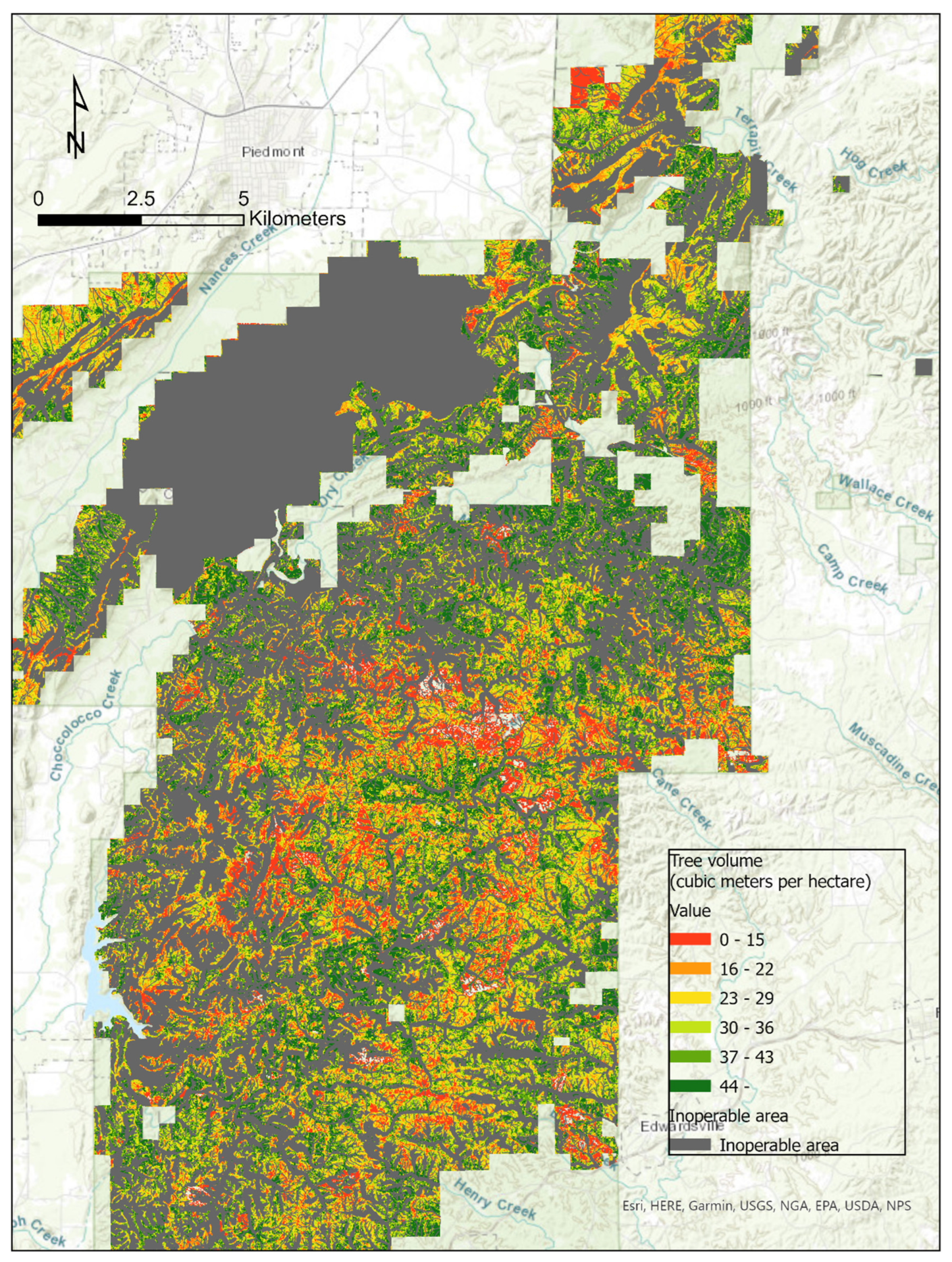
Figure 6.
Estimated aboveground biomass for a portion of the study area based on general model (Sources: Esri. “World Topographic Map” [basemap]. January 31, 2024).
Figure 6.
Estimated aboveground biomass for a portion of the study area based on general model (Sources: Esri. “World Topographic Map” [basemap]. January 31, 2024).
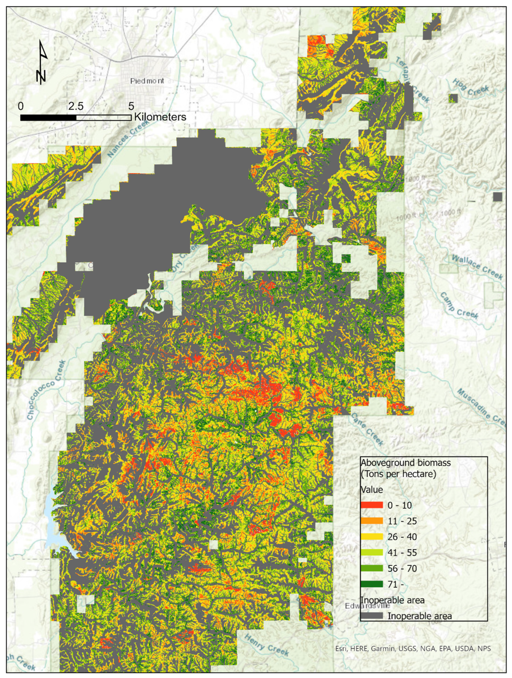

Table 1.
Summary of vegetation indices calculated from the NAIP images.
| Vegetation Index | Equation | Calculated statistics and its abbreviation |
| Greenness | Minimum of greenness (GMIN) | |
| Maximum of greenness (GMAX) | ||
| Range of greenness (GRANGE) | ||
| Mean of greenness (GMEAN) | ||
| Standard deviation of greenness (GSTD) | ||
| Sum of greenness (GSUM) | ||
| Median of greenness (GMEDIAN) | ||
| 90 percentage of greenness (GPCT90) | ||
| Normalized Difference Vegetation Index, NDVI | Minimum of NDVI (NDVIMIN) | |
| Maximum of NDVI (NDVIMAX) | ||
| Range of NDVI (NDVIRANGE) | ||
| Mean of NDVI (NDVIMEAN) | ||
| Standard deviation of NDVI (NDVISTD) | ||
| Sum of NDVI (NDVISUM) | ||
| Median of NDVI (NDVIMEDIAN) | ||
| 90 percentage of NDVI (NDVIPCT90) | ||
| Enhanced Vegetation Index, EVI | Minimum of EVI (EVIMIN) | |
| Maximum of EVI (EVIMAX) | ||
| Range of EVI (EVIRANGE) | ||
| Mean of EVI (EVIMEAN) | ||
| Standard deviation of EVI (EVISTD) | ||
| Sum of EVI (EVISUM) | ||
| Median of EVI (EVIMEDIAN) | ||
| 90 percentage of EVI (EVIPCT90) |
*Where R, G, B, NIR represent the raw pixel values of red, green, blue, and the near-infrared bands.
Table 2.
Summary of the independent variables derived from LiDAR point cloud.
| Metrics | Descriptions | Metrics | Descriptions |
| zmean | Mean height | zpcum x (from 1st to 9th) |
Cumulative percentage of return in the ith layer |
| zsd |
Standard deviation of height distribution | isd | standard deviation of intensity |
| zskew |
Skewness of height distribution | iskew | skewness of intensity distribution |
| zkurt | Kurtosis of height distribution | ikurt | kurtosis of intensity distribution |
| zentropy | Entropy of height distribution | ipground | percentage of intensity returned by points classified as "ground" |
| pzabovezmean | Percentage of returns above z mean | ipcumzq x (10th, 30th, 50th, 70th, and 90th) |
Percentage of intensity returned below the xth percentile of height |
| Pzabove2 |
Percentage of returns above 2 m | P xth (1, 2, 3, 4, and 5) |
Percentage xth returns |
| zq x (From 5th to 95th) |
xth percentile (quantile) of height distribution | pground | Percentage of returns classified as "ground" |
Table 3.
Descriptive statistics of forest attributes based on field measurements.
| Diameter at breast height (cm) | Basal area (m2 ha-1) | Volume (m3 ha-1) | Aboveground biomass (Mg ha-1) | |
| All plots (n =254) | ||||
| Average | 22.39 | 23.43 | 180.85 | 40.13 |
| Standard deviation | 7.39 | 10.95 | 105.48 | 23.07 |
| Minimum | 8.65 | 0.33 | 0.77 | 0.13 |
| Maximum | 54.36 | 53.29 | 569.93 | 119.03 |
| Pine plots (n =149) | ||||
| Average | 22.42 | 22.28 | 168.97 | 34.62 |
| Standard deviation | 8.40 | 16.92 | 108.26 | 21.94 |
| Minimum | 8.66 | 0.33 | 0.77 | 0.13 |
| Maximum | 54.36 | 51.19 | 543.27 | 110.02 |
Table 4.
The best equations for the general (all plots, n=254) and the pine (pine plots, n=149) models by forest attribute and data sources.
Table 4.
The best equations for the general (all plots, n=254) and the pine (pine plots, n=149) models by forest attribute and data sources.
| Forest variables | Data sources | eequation |
| General models | ||
| Basal area | LiDAR+ NAIP | -1.828 + 0.017 * pzabove2 + 0.015 * zq25 + 0.017 * zq95 - 7.83 * e-4 * zpcum5 - 0.002 * zpcum6 + 2 * e-5 * isd + 0.24 * iskew - 0.091 * ikurt + 0.024 * ipcumzq90 + 0.043 * p2th + 0.116 * GMIN + 0.52 * NDVIMIN + 0.428 * NDVIMEDIAN + 3.58 * e-5 * EVIMAX - 0.012 * EVIPCT90 |
| LiDAR | -1.197 + 0.018 * pzabove2 + 0.017 * zq25 + 1.13 * e-4 * zq30 + 0.015 * zq95 - 3.79 * e-4 * zpcum5 - 0.003 * zpcum6 + 1.83 * e-5 * isd + 0.196 * iskew - 0.105 * ikurt + 0.017 * ipcumzq90 + 0.046 * p2th | |
| Volume | LiDAR+ NAIP | -0.148 + 0.018 * pzabove2 + 0.004 * zq25 + 0.056 * zq95 - 7.91 * e-4 * zpcum5 - 0.00566 * zpcum6 + 2.51 * e-5 * isd + 0.237 * iskew - 0.128 * ikurt - 0.018 * ipcumzq10 - 0.002 * ipcumzq30 + 0.029 * ipcumzq90 - 0.002 * p1th + 0.029 * p2th + 0.091 * GMIN - 0.165 * GRANGE + 0.522 * NDVIMIN + 0.229 * NDVIMEAN + 1.45 * e-5 * NDVISUM + 0.158 * NDVIMEDIAN + 1.96 * e-4 * EVIMAX - 0.010 * EVIPCT90 |
| LiDAR | 0.380 + 0.020 * pzabove2 + 0.007 * zq25 + 0.053 * zq95 - 0.006 * zpcum6 + 3.088 * e-05 * isd + 0.209 * iskew - 0.121 * ikurt - 0.020 * ipcumzq10 - 0.004 * ipcumzq30 + 0.020 * ipcumzq90 - 4.642 * e-5 * p1th + 0.037 * p2th | |
| Aboveground biomass | LiDAR+ NAIP | 0.033 + 0.021 * pzabove2 + 0.062 * zq95 - 0.004 * zpcum6 + 3.93 * e-5 * isd + 0.132 * iskew - 0.184 * ikurt - 0.011 * ipcumzq10 + 0.083 * ipcumzq90 - 0.006 * p1th + 0.031 * p2th - 1.51 * e-4 * pground + 0.385 * GMIN + 0.505 * NDVIMIN + 0.218 * NDVIMEAN + 9.36 * e-6 * NDVISUM - 0.005 * EVIPCT90 |
| LiDAR | 0.516 + 0.022 * pzabove2 + 0.238 * zq5 + 0.002 * zq25 + 0.059 * zq95 - 0.005 * zpcum6 + 3.83 * e-5 * isd + 0.103 * iskew - 0.198 * ikurt - 0.012 * ipcumzq10 + 0.078 * ipcumzq90 - 0.006 * p1th + 0.034 * p2th | |
| Pine models | ||
| Basal area | LiDAR+ NAIP | 0.657 + 0.009 * pzabove2 + 3.600 * zq5 + 0.021 * zq25 + 0.001 * zq40 + 0.007 * zq95 - 0.009 * zpcum5 + 0.173 * iskew - 0.067 * ikurt + 0.057 * p2th + 0.426 * NDVIMIN + 0.985 * NDVIMEDIAN - 8.6 * e-4 * EVIPCT90 |
| LiDAR | 5.195 + 0.011 * pzabove2 + 2.873 * zq5 + 0.021 * zq25 + 1.681 * e-4 * zq40 + 0.003 * zq95 - 0.008 * zpcum5 - 1.96 * e-4 * zpcum6 + 0.168 * iskew - 0.061 * ikurt - 0.004 * ipcumzq30 - 0.0475 * ipcumzq90 + 0.057 * p2th | |
| Volume | LiDAR+ NAIP | 1.593 - 0.002 * zkurt + 0.021 * pzabove2 + 8.41 * zq5 - 1.91 * zq15 + 0.019 * zq25 + 0.006 * zq40 - 0.008 * zq65 + 0.016 * zq75 - 0.071 * zq80 + 0.096 * zq95 + 0.010 * zpcum1 - 0.010 * zpcum5 - 0.005 * zpcum6 + 1.29 * e-5 * zpcum8 + 0.002 * zpcum9 + 3.04 * e-5 * isd + 0.241 * iskew - 0.16 * ikurt + 0.016 * ipcumzq10 - 0.008 * ipcumzq30 + 0.042 * p2th - 0.039 * p5th + 0.486 * GMIN - 0.132 * GRANGE + 0.475 * NDVIMIN + 1.28 * NDVIMEDIAN + 2.7 * e-4 * EVIMAX - 0.004 * EVISTD - 0.019 * EVIMEDIAN - 0.015 * EVIPCT90 |
| LiDAR | 3.592 + 0.008 * pzabove2 + 3.401 * zq5 + 0.004 * zq25 + 0.043 * zq95 - 0.013 * zpcum5 + 0.222 * iskew - 0.094 * ikurt - 2.769 *e-4 * ipcumzq10 - 0.033 * ipcumzq30 + 0.047 * p2th + 0.013 * p3th | |
| Aboveground biomass | LiDAR+ NAIP | 6.466 - 0.005 * zkurt + 0.41 * zentropy + 0.025 * pzabove2 + 8.66 * zq5 - 0.037 * zq10 - 2.18 * zq15 + 0.017 * zq25 - 7.48 *e-4 * zq30 + 0.004 * zq40 - 0.001 * zq65 + 0.010 * zq75 - 0.079 * zq80 + 0.11 * zq95 + 0.013 * zpcum1 - 0.009 * zpcum5 - 0.005 * zpcum6 + 0.003 * zpcum9 + 4.75 * e-05 * isd + 0.078 * iskew - 0.175 * ikurt + 0.020 * ipcumzq10 - 0.008 * ipcumzq90 + 0.042 * p2th - 0.016 * p5th + 0.673 * GMIN - 0.094 * GRANGE + 0.171 * GSTD - 0.362 * GMEDIAN + 0.364 * NDVIMIN - 0.327 * NDVISTD + 1.51 * NDVIMEDIAN + 1.52 *e-4 * EVIMAX - 0.002 * EVISTD - 0.033 * EVIPCT90 |
| LiDAR | 10.699 + 0.013 * pzabove2 + 2.062 * zq5 + 0.052 * zq95 - 0.011 * zpcum5 + 0.010 * iskew - 0.129 * ikurt - 0.010 * ipcumzq30 - 0.024 * ipcumzq90 - 0.009 * p1th + 0.045 * p2th | |
Table 5.
Summary of statistics for the general models.
| Quality metrics | Basal area (m2 ha-1) | Total volume (m3 ha-1) | Total aboveground biomass (Mg ha-1) | |||
| LiDAR + NAIP | LiDAR | LiDAR + NAIP | LiDAR | LiDAR + NAIP | LiDAR | |
| R2adj. | 0.72 | 0.71 | 0.77 | 0.77 | 0.73 | 0.72 |
| # of variables | 15 | 11 | 21 | 12 | 16 | 12 |
| RMSE | 5.58 | 5.73 | 48.44 | 49.34 | 11.68 | 11.84 |
| R2 | 0.74 | 0.72 | 0.79 | 0.78 | 0.74 | 0.74 |
| Bias | - 0.78 | -0.80 | -6.27 | -6.54 | -1.62 | -1.64 |
| Bias (%) | -3.33 | -3.40 | -3.45 | -3.61 | -4.03 | -4.08 |
| AIC | 0.08 | -76.05 | -118.05 | -137.76 | -137.43 | -145.17 |
| BIC | -68.19 | -38.28 | -47.95 | -96.66 | -83.13 | -104.02 |
| CP | -17.21 | 0.08 | 0.11 | 0.12 | 0.12 | 0.13 |
Table 6.
Analysis of 10-fold cross-validation for the general regression models.
| Quality metrics | Basal area (m2 ha-1) | Total volume (m3 ha-1) | Total aboveground biomass (Mg ha-1) | |||
| LiDAR + NAIP | LiDAR | LiDAR + NAIP | LiDAR | LiDAR + NAIP | LiDAR | |
| R2adj. | 0.69 | 0.71 | 0.67 | 0.73 | 0.64 | 0.65 |
| R2 | 0.72 | 0.69 | 0.72 | 0.75 | 0.69 | 0.68 |
| RMSE | 5.90 | 5.91 | 55.87 | 53.10 | 13.05 | 13.09 |
| Bias | -0.76 | -0.75 | -4.06 | -7.56 | -1.12 | -1.21 |
| Bias (%) | -3.20 | -3.20 | -2.26 | -4.12 | -2.63 | -2.85 |
Table 7.
The most important independent variables of the best regression models.
| LiDAR metrics | NAIP metrics | |
| General & pine model | pzabove2, zq95, iskew, ikurt, p2th | NDVIMIN, EVIPCT90 |
| General model | zpcum6, isd, ipcumzq90 | GMIN |
| Pine model | zq5, zpcum5 | NDVIMEDIAN |
Table 8.
Summary of statistics for the pine regression models.
| Quality metrics | Basal area (m2 ha-1) | Total volume (m3 ha-1) | Total aboveground biomass (Mg ha-1) | |||
| LiDAR + NAIP | LiDAR | LiDAR + NAIP | LiDAR | LiDAR + NAIP | LiDAR | |
| R2adj. | 0.81 | 0.80 | 0.84 | 0.82 | 0.83 | 0.82 |
| # of variables | 12 | 12 | 30 | 11 | 34 | 10 |
| RMSE | 4.80 | 5.10 | 37.86 | 43.45 | 7.89 | 8.93 |
| R2 | 0.83 | 0.81 | 0.87 | 0.84 | 0.87 | 0.83 |
| Bias | -0.72 | -0.75 | -3.65 | -6.71 | -0.68 | -1.36 |
| Bias (%) | -3.23 | -3.38 | -2.12 | -3.92 | -1.93 | -3.89 |
| AIC | -5.84 | -54.77 | -56.60 | -108.83 | -49.23 | -113.69 |
| BIC | -22.09 | -21.01 | 17.08 | -77.80 | 31.20 | -85.33 |
| CP | 0.07 | 0.08 | 0.06 | 0.11 | 0.06 | 0.10 |
Table 9.
Analysis of 10-fold cross-validation for the pine regression models.
| Quality metrics | Basal area (m2 ha-1) | Total volume (m3 ha-1) | Total aboveground biomass (Mg ha-1) | |||
| LiDAR + NAIP | LiDAR | LiDAR + NAIP | LiDAR | LiDAR + NAIP | LiDAR | |
| R2adj. | 0.79 | 0.75 | 0.78 | 0.79 | 0.80 | 0.78 |
| R2 | 0.82 | 0.78 | 0.82 | 0.81 | 0.84 | 0.81 |
| RMSE | 5.21 | 5.71 | 47.44 | 48.94 | 9.42 | 10.24 |
| Bias | -0.72 | -0.99 | -4.41 | -8.43 | -0.97 | -0.92 |
| Bias (%) | -3.17 | -4.33 | -2.48 | -4.92 | -2.21 | -2.71 |
Disclaimer/Publisher’s Note: The statements, opinions and data contained in all publications are solely those of the individual author(s) and contributor(s) and not of MDPI and/or the editor(s). MDPI and/or the editor(s) disclaim responsibility for any injury to people or property resulting from any ideas, methods, instructions or products referred to in the content. |
© 2024 by the authors. Licensee MDPI, Basel, Switzerland. This article is an open access article distributed under the terms and conditions of the Creative Commons Attribution (CC BY) license (http://creativecommons.org/licenses/by/4.0/).
Copyright: This open access article is published under a Creative Commons CC BY 4.0 license, which permit the free download, distribution, and reuse, provided that the author and preprint are cited in any reuse.


