
Submitted:
09 June 2025
Posted:
09 June 2025
You are already at the latest version
Abstract
This article presents a hybrid mathematical model to address the interaction between transmission and energy generation expansion in response to dynamically increasing energy demand. By employing linear programming for optimal power flows, the proposed co-optimization model simultaneously solves the expansion of both the generation facilities and the transmission system in a single stage. Consequently, it enables the minimization of investment and operating costs for both new and existing generators, the investment costs of new components added to the transmission network, and the cost of unsupplied energy. The formulated optimization model is applied to a standard [purpuragrisacea]IEEEInstitute of Electrical and Electronics Engineers. 14-bus power system under dynamic load scenarios with growth rates corresponding to expansion periods of two and five years.
Keywords:
Power system planning
; Generation expansion
; Transmission network expansion
; Simultaneous expansion planning
; Mixed-Integer Nonlinear Programming (MINLP)
; Dynamic load scenarios
; Optimal Power Flow (OPF)
1. Introduction
Electricity consumption is steadily increasing, driven by the degree of technological innovation across various commercial and industrial processes. Consequently, electricity generation sources must be sufficient and reliable to ensure sustainable and productive economic progress. While a large part of the world has access to electric power services, it cannot be guaranteed that this energy is delivered with high quality standards, due to energy crises experienced in different regions. This situation, at least partially, stems from inadequate expansion of power systems to meet future demand requirements [1].
In power systems (PS), both the integration of various electricity generation technologies and the implementation of networks that enhance supply reliability can provide solutions to several challenges faced by modern electrical systems. These challenges include power quality issues, voltage instability, electrical losses, and environmental pollution. Such problems arise because power networks were not originally designed to accommodate the technological innovations that have emerged over time in the generation and transmission stages. Therefore, it is essential to focus on planning the expansion of generation facilities and transmission networks to enable effective adaptation of the resources available in the electrical grid [2].
Expansion problems are typically addressed in two interrelated but independent stages aimed at meeting demand and its growth over a given time horizon [3]. The first stage corresponds to Generation Expansion Planning (GEP), which determines generation requirements, and the second to Transmission Expansion Planning (TEP), which specifies network requirements or reinforcements [4,5]. Each stage considers distinct technical and economic conditions and can be formulated as an optimization problem with the objective of minimizing or maximizing a function based on a mathematical approach [6]. As energy needs become increasingly demanding, additional tools and expertise are required to resolve the challenges involved in managing the PS as a whole. This has led to the evolution of power system planning models and tools that integrate generation expansion and transmission growth to act in coordination. This integrated approach helps mitigate network issues arising from the high penetration of generation in response to dynamically growing demand [4,7].
Integrated or simultaneous generation and transmission expansion planning (IGTEP) aims to identify the most cost-effective plan for determining the power capacity to be added, the type of generation and transmission required, the timing of investments, and the optimal locations for generation plants and transmission lines. This planning ensures that projected demand is met while complying with system constraints and required reliability levels [8].
In an effort to develop IGTEP models that reflect the real conditions of power systems, several studies have proposed approaches focused on maximizing social welfare, as seen in [9]. Other works, such as [10], have considered security constraints. In [11], both investment and operating costs were minimized, while [12] analyzed the effects of uncertainty in primary energy sources and their prices. In contrast, [13] addressed renewable energy penetration, and [12] explored losses and reactive power using AC and DC network models. These and other studies have emphasized the benefits of combining generation and transmission planning into unified objective functions under appropriately defined constraints.
Current research on IGTEP explores various methods grouped into two main categories, each with its own set of programming tools, whose application depends on computational limitations. The first category is based on mathematical optimization. For instance, some studies have formulated the IGTEP problem using Mixed-Integer Linear Programming (MILP) [14], linear programming [15], and MILP-based co-optimization approaches [16]. The second category involves metaheuristic algorithms. Notable examples include combined expansion planning with Monte Carlo simulation models [17], the use of Benders decomposition [18], stochastic algorithms [19], genetic algorithms [20], and hybrid methods integrating genetic algorithms with gradient-based techniques for IGTEP [21]. These studies present a variety of methodologies capable of solving simultaneous expansion planning problems. Such methodologies foster a large number of studies because IGTEP results tend to be satisfactory, ensuring both the overall minimization of costs and the fulfillment of projected demand within the defined planning horizon.
This research proposes a novel method for the simultaneous expansion of the generation stage and the transmission network using AC power flow models. The expansion is formulated as an optimization problem through Mixed-Integer Nonlinear Programming (MINLP). The innovation of the proposed model lies in the continuous and intensive interaction involved in solving n nonlinear programming problems for the modeled system. These problems, governed by the electrical laws of AC power flows, determine the inclusion of new generation units and possible new links in the network. The AC power flows, which include both active and reactive power, as well as voltage levels, are treated as variables that must remain within technical limits to guarantee reliability, continuity, and quality in steady-state operation of the system over the medium and long term. The objective of this work is to minimize the investment costs of new generators and newly added transmission elements, the operating costs of both existing and new generation units, and the CENS. The formulated model considers multiple dynamic load scenarios to evaluate the technical and economic aspects associated with the simultaneous expansion of the generation park and the transmission system in a test network. Therefore, the proposed model provides optimal investment strategies for sizing, siting, and scheduling new investments in generation units and interconnection networks to meet the forecasted demand.
linkcolor=myDarkRedThis article is organized as follows: Section 2 analyzes the criteria for integrated expansion planning, along with the model and solution methods used for IGTEP. Section 3 formulates the objective function and constraints of the proposed IGTEP methodology. Section 4 presents the case studies. Section 5 discusses the results, and finally, Section 6 provides the conclusions of this research.
2. Integrated Planning for Power System Expansion
Expansion planning in power systems is a complex study aimed at determining the optimal way to expand generation, distribution, and transmission in order to meet consumers’ energy needs at the lowest possible cost over a defined time horizon [22]. While the primary objective is to meet demand, the delivery of electricity must also be reliable, secure, and economical, considering the technical, economic, and political aspects involved in the power grid [23]. Traditionally, expansion planning has focused on generation due to the high investment costs it entails compared to transmission network expansion. It is worth noting that distribution also requires considerable investment, but in large part, this is the responsibility of entities other than those involved in production and transmission [24,25].
The relationship between producer and consumer needs results in combined variables that highlight the necessity for tools that integrate the apparent separation between generation and transmission planning [26]. However, in practice, generation is typically planned and scheduled based on demand growth, thereby providing guidelines for the transmission network’s expansion plan. Generation planning is based on assumptions about load growth at the distribution stage, which means that each planning process is treated separately due to the fragmented decisions made by investors and operators—ultimately leading to disorder in system expansion and reduced overall economic benefits [27].
Therefore, considering the interdependence between generation and transmission expansion—and the significant investments both require—it is essential to adopt an integrated planning approach that justifies the new infrastructure from both a technical and economic standpoint, since such developments have a direct impact on all users of the system. This issue has been the subject of limited research and is known as Integrated Generation and Transmission Expansion Planning [28]. IGTEP is a process that employs various methodologies and models to coordinate expansion plans simultaneously, with the goal of determining the location, quantity, and type of generation and transmission units to be added to the power system at the appropriate time, ensuring that projected demand is met at minimum cost and under reliable conditions [29].
2.1. Criteria for Integrated Expansion Planning
The formulation of the IGTEP problem involves several criteria distributed across different stages, enabling effective system integration for electricity supply. Moreover, these criteria impact the complexity of the modeling process due to the number of variables and data involved, which can lead to challenges in data processing and computation. Therefore, robust computational tools are required to handle this type of analysis. The following section presents these criteria in a general manner.
2.1.1. Demand Growth
Electric power systems evolve in efficiency and structure according to demand behavior. Their adaptation depends on energy consumption, which is complex to measure due to its high level of uncertainty [30]. For this reason, over time, various methods have been developed and refined to forecast the dynamic behavior of demand and to establish corresponding growth rates. These forecasts serve as the foundation for power system studies within their respective time frames. Therefore, demand contributes to expansion planning by incorporating load growth rates, particularly exponential growth rates applicable at the continental (American) level [31].
2.1.2. Generation Expansion Planning
GEP generally determines the entry, size, and optimal location of new power generation units while minimizing total cost over a medium- or long-term planning horizon. Generation expansion typically adopts an energy-focused approach and disregards transmission network constraints [32]. Therefore, to address the IGTEP problem, it is essential to consider the active and reactive power contributions of the generators, plant capacity factors, investment and operational costs of generation facilities, and the location and capacity of the units involved in the expansion plan.
2.1.3. Transmission Expansion Planning
TEP refers to the installation of new transmission lines or the expansion of the capacity of existing lines within a power system [10]. Transmission expansion planning identifies the network reinforcements required to ensure energy delivery to system users at minimum cost, while also pinpointing the supply points established by GEP. The criteria that TEP must consider for integrated planning focus on link-related characteristics, such as line investment and operating costs, network topology, line loading capacity, operating voltage levels, and active and reactive power flow.
2.1.4. Unsupplied Energy
This criterion is incorporated when the generation resources or transmission infrastructure are unable to meet the demand during the period in which the expansion is evaluated.
2.2. Model and Solution Method for IGTEP
To perform a combined expansion study, it is necessary to define a mathematical model capable of incorporating the previously mentioned criteria. For this study, the model considers the expansion of both the generation and transmission stages, while also applying AC power flow equations. Solving these equations enables a highly accurate approximation of the real operation of power systems, despite the mathematical complexity introduced by the nonlinearities of the load flow equations [33]. These equations are characterized by voltage, angle, active power, and reactive power variables, which determine the flows in the transmission network based on generation and demand levels [28,34].
The power flow model in this work is based on the following assumptions: the technical and economic characteristics of generators and transmission lines are known; new transmission lines have the same characteristics as existing ones; growing demand—which drives the need for system expansion—is represented through dynamic load scenarios based on growth rates; and Energy Not Supplied (ENS) is assigned a value when generation resources or transmission infrastructure are insufficient to meet demand over a given period.
For the formulation of load flow studies within the integrated expansion plan, it is essential to define a methodology that satisfies the objective function of minimizing costs (investment, operating, and ENS) by optimally deploying new generation and reinforcing the transmission network according to demand growth. A variety of solution methods exist, ranging from metaheuristic algorithms to classical mathematical optimization methods, each with its own advantages and limitations [35]. Considering the challenges posed by generation and transmission expansion planning, this work uses a mathematical co-optimization algorithm based on MINLP. This approach is suitable due to the nonlinear nature of the equations, the non-convexity arising from decision variables inherent to electrical laws, and the large scale of the problem. The selected algebraic modeling approach enables the simultaneous identification of the best expansion alternatives for generation units and the transmission network to meet future demand, using a minimum-cost criterion for both operation and investment.
3. Methodology for the Simultaneous Expansion of Generation and Transmission
The simultaneous expansion of the generation and transmission stages of the power system is obtained by solving a MINLP model, which involves binary decision variables and mixed-type variables. Their interaction enables the determination of the new infrastructure required in the aforementioned segments of the power sector.
3.1. Objective Function
The objective function is divided into three components: the first corresponds to the costs associated with the generation park, the second relates to the costs of the new transmission system infrastructure, and the third evaluates the ENS.
3.1.1. Generation Park Costs
3.1.2. Transmission Infrastructure Costs
3.1.3. Costs of Energy Not Supplied
ENS occurs when the generation system is unable to meet demand. This shortage results in a significant cost to consumers and is modeled in (6).
3.2. Constraints
The constraints in the model correspond to the technical aspects of the power system, including the modeling of AC power flows, operational characteristics of generators, interconnection link capacity limits, and their implications for the associated variables.
3.2.1. Flows in Transmission Network Links
This constraint associates the variable with the AC power flow equations. In this case, both active and reactive power must be modeled. For this purpose, the Big M method is used [36,37], which is based on associating constraints with large negative constants that would not be part of any optimal solution. When applying the Big M method in constraints, it ensures that variable enforcement occurs only when a defined binary variable takes on a specific value, while leaving the variables "open" if the binary variable takes the opposite value.
3.2.2. Power Transfer Limits of the Links
The transfer limits on the links are related to the maximum or minimum amount of active or reactive power that can be transferred through a given link, whether it is an existing or a new one. The transferred power must not exceed the thermal or loading limit of the link.
3.2.3. Bidirectionality of Decision Variables for the New Link
This constraint ensures that the decision to incorporate a new link between two nodes is not duplicated and does not have an additional impact on the investment cost of the new transmission infrastructure.
3.2.4. Nodal Balance
The formulation of the nodal balance is applicable to the active and reactive power at each node of the power system and must comply with the concept established by Kirchhoff’s First Law.
3.2.5. Capacity of New Generators
This constraint allows the incorporation of a generation plant based on demand requirements and its growth through the use of a binary decision variable.
3.2.6. Generation Output Limits
This constraint ensures that the active and reactive power dispatched by any generator does not exceed the limits defined by the generator capability curve.
3.2.7. Nodal Voltage Limits
This constraint ensures that the nodal voltages in per unit remain within the defined range to guarantee voltage stability in the system.
3.2.8. Nodal Angle Limits
This constraint ensures that the voltage angles at the nodes remain within the specified range, thereby maintaining angular stability in the system.
3.2.9. Optimization Model Pseudocode
By solving the proposed mixed-integer nonlinear optimization model, the expansion of new links in the transmission system can be determined, and simultaneously, the new generation plants to be incorporated into the system are obtained, all while minimizing the costs associated with the generation and transmission stages.
The decision to expand the generation and transmission stages not only considers minimizing associated costs but also takes into account relevant aspects, such as network constraints — the application of power flow equations and their implications for link loading. It also incorporates the application of the Big M method, which facilitates the decision to include new links, directly impacting the need to incorporate new generations. The decision to incorporate is provided by binary variables, which resolve the inclusion of generation and transmission elements, ensuring the supply of demand and consequently the fulfillment of link loading constraints and voltage level requirements.
Representation 1 presents the pseudocode of the proposed heuristic.
4. Case Studies
The proposed mixed-integer nonlinear programming mathematical model was applied to the IEEE 14-bus system, as illustrated in Figure 1. To evaluate the mathematical model, the following case studies are considered:
- : Expansion of the model power system in the generation and transmission stages for a period of 2 years.
- : Expansion of the model power system in the generation and transmission stages for a period of 5 years.
Each case uses dynamic load scenarios, increasing demand exponentially at annual rates of 5%, 7%, and 9%. Accordingly, three analyses will be conducted for each case described. Table 1 presents the characteristics of the power system network used as a model [38].
5. Results Analysis
Given the described cases and the dynamic load scenarios applied to each one, the results are evaluated from both technical and economic perspectives.
5.1. Case 1
By applying the mathematical model over a 2-year analysis period for each dynamic load scenario, the results of the electrical and economic variables are obtained. Generation and demand are evaluated, as presented in Table 6. Figure 2 illustrates the results of active generation and supplied demand, including the corresponding losses.
The results show that, for each analyzed load scenario, the operating generation fleet—with a nominal capacity of 350 MW—is sufficiently robust to supply the demand and meet the network’s operational requirements. Therefore, the model indicates that no generation expansion is required.
On the other hand, when evaluating active power losses in relation to the supplied demand for each load scenario, it is concluded that the average percentage of losses amounts to 2.84%.
Table 7 presents the results for reactive power. The analysis reveals that the total reactive power capacity produced by the generators is 238 Mvar, which supplies the increased load and compensates for network losses without the need to increase generation. The results are illustrated in Figure 3.
An evaluation of reactive power losses relative to the supplied demand in each load scenario shows that the average loss percentage amounts to 6.59%. Given that reactive power production is directly related to voltage levels, voltage profiles at the end of the analysis period are verified for each dynamic load scenario, as illustrated in Figure 4.
Figure 4 shows that for all demand growth scenarios, voltage levels remain within the operational band, ensuring voltage stability across the system. To complement the technical analysis, the transmission network expansion is also examined. The results of this verification are presented in Table 8.
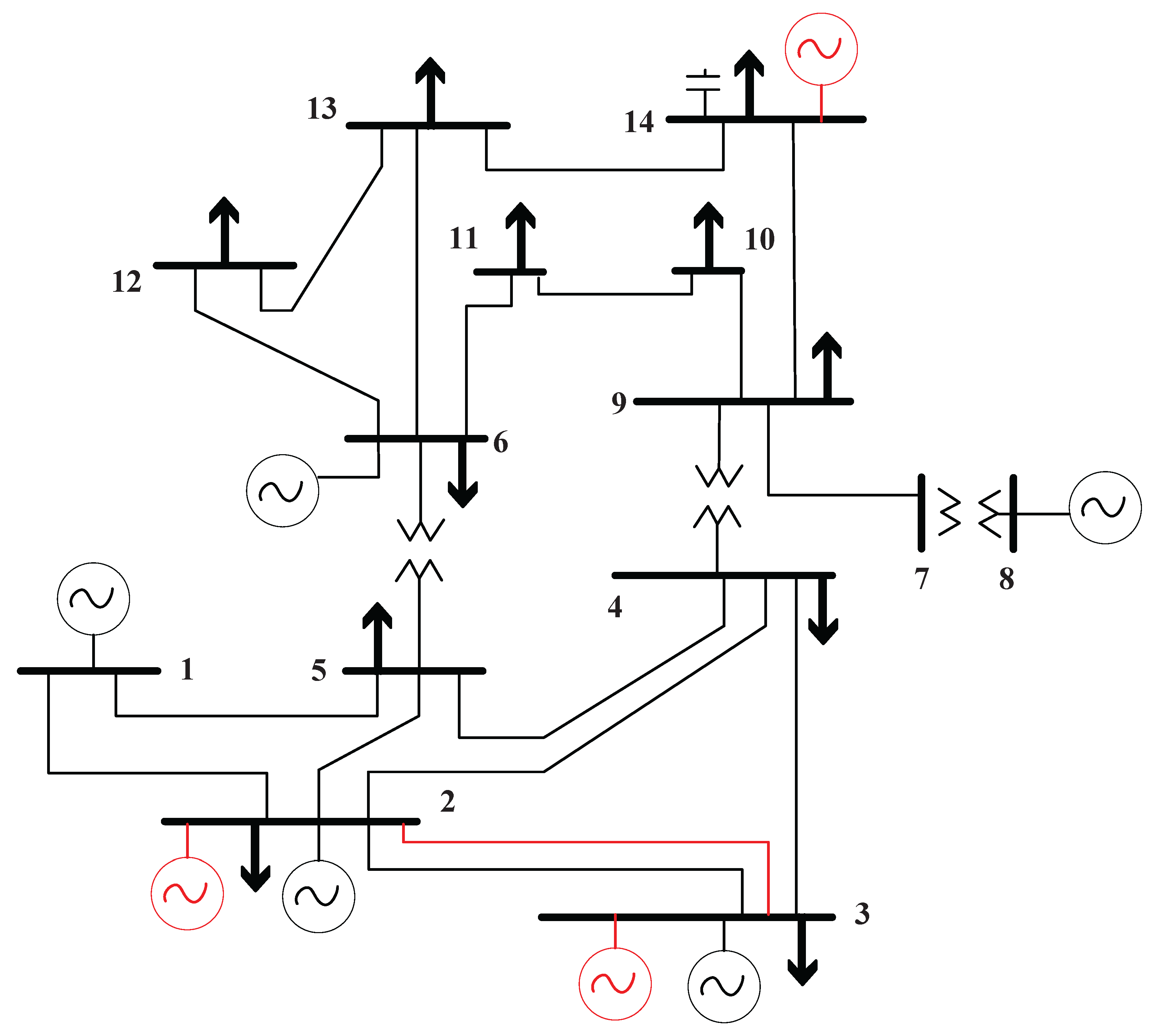
Based on Table 8, it is concluded that although no expansion of the generation system is required—since the installed capacity is sufficient to supply the demand—the model indicates the need to reinforce the transmission system. For this case, regardless of the load scenario, the link connecting node 4 to node 9 is activated, corresponding to the expansion of a substation, and a new transmission line is added between nodes 2 and 3. Figure 5 shows the single-line diagram of the expanded electrical system for all load scenarios.
The resulting voltages for each load scenario are listed in Table 9, while power flows through each link of the simulated network for every load scenario are presented in Appendix A.
Based on the results of the electrical variables, the operating costs of energy production from the operating generation, as well as the annualized investment costs of the incorporated links, are determined. The costs for each load scenario in Case 1 are presented in Table 10.
5.2. Case 2
For a 5-year analysis period under each dynamic load scenario, the results of the electrical and economic variables are obtained. Analogous to Case 1, production and demand are evaluated, and the results are presented in Table 11. Figure 6 illustrates the results of active power generation and supplied demand, including the corresponding losses.
From the results for each analyzed load scenario, it can be concluded that the existing generation fleet must be expanded in order to meet the demand and fulfill the network’s operational requirements. Therefore, the results of the generation expansion are presented in Table 12.
Considering the analysis period and the associated increase in load, it can be stated that the new generation along with the existing generation enables the system to meet the demand and compensate for active power losses. In this context, the average percentage of active power losses with respect to the supplied demand across the load scenarios reaches a value of 2.61%.
Similarly, a reactive power analysis is carried out. The results are shown in Table 13, from which it can be observed that the model performs an allocation of reactive power between the new and existing generators. This allocation not only supplies the increased load but also compensates for losses occurring in the network. The results are illustrated in Figure 7.
Based on the results obtained for each analyzed load scenario, as previously indicated, the existing generation fleet must be expanded to meet demand and satisfy the network’s operational requirements. Accordingly, the results of the generation expansion are presented in Table 14.
As a complement, by evaluating the reactive power losses relative to the supplied demand for each load scenario, it is observed that the average percentage of losses amounts to 8.90%. In this regard, since reactive power production is directly related to voltage levels, voltage profiles are verified at the end of the analysis period for each load scenario, as illustrated in Figure 8.
From Figure 8, it is evident that in all demand growth scenarios, the voltage levels remain within the operational band. This ensures that the system maintains its voltage stability. To complement the technical analysis, the network expansions are verified; the verification results are presented in Table 15.
From Table 15, it is concluded that, except for the 5% demand growth scenario, network expansions are implemented; even though generation expands in all demand scenarios. In this case, the model indicates the need to reinforce the transmission system, activating the new link connecting node 2 and node 3. Figure 9 and Figure 10 show the one-line diagrams of the expanded power system.
The voltage results for each load scenario are shown in Table 16, and the power flows for each network link in the simulated grid are presented in Appendix B.
Taking into account the results of the electrical variables, the operating costs of the power generation from the existing generators are determined, along with the annualized investment costs of the incorporated links. These results are presented in Table 17.
6. Conclusions
The proposed nonlinear mixed-integer optimization model enables the simultaneous expansion of both the generation stage and the transmission system in order to meet demand using optimal AC power flows. This approach makes it possible to determine the power delivered by new generation units and new network links—two components which, when interacting, ensure economic supply of demand over the analysis period. All of this is done while considering the constraints associated with the operational characteristics of the PS
Based on the results obtained for each case study and considering the dynamic load scenarios, it can be stated that when the analysis period is shorter, the model prioritizes network investments and optimization of the existing generation resources to minimize associated costs while still complying with network constraints, as evidenced in the results of Case 1. Likewise, as the analysis period increases and demand grows significantly, the model introduces new generation and transmission links simultaneously into the electric system—an outcome reflected in the results of Case 2. Therefore, it is confirmed that the model achieves simultaneous expansion of the generation park and transmission system, while also modeling network-specific constraints.
The decisions to expand generation capacity or to include new transmission links consider the system’s technical constraints but, more importantly, take into account the associated costs. Consequently, it is concluded that careful incorporation of unit cost data is essential to ensure that the model produces consistent results and accurately determines required investments. Otherwise, poor planning could lead to overcosts that, depending on the market structure in each country, must be compensated—typically resulting in increased tariffs for the end user.
The proposed mathematical model integrates the nonlinear conditions of AC power flow with binary variables that define investment decisions in both generation and transmission. Furthermore, its formulation is scalable and adaptable to various electric systems, making it a valuable tool for short-, medium-, and long-term planning.
Since the model proposes a novel methodology for the simultaneous expansion of generation and transmission stages, it is recommended that future work includes a stochastic analysis comparing the classical methodology with the approach presented herein, in order to establish technical and economic parameters that allow the electric system to optimally serve demand over the medium and long term.
Appendix A. Power flows through the network, Case 1
Appendix A.1. Active power flow 1

Table A1.
Active power flow [MW].
| 5% | 7% | 9% | ||
| 1 | 2 | 102.42 | 102.26 | 102.61 |
| 1 | 5 | 57.58 | 57.74 | 57.39 |
| 2 | 1 | -100.43 | -100.26 | -100.60 |
| 2 | 3 | 72.00 | 71.17 | 71.28 |
| 2 | 4 | 47.30 | 46.72 | 46.55 |
| 2 | 5 | 37.20 | 37.53 | 36.99 |
| 3 | 2 | -70.81 | -70.01 | -70.11 |
| 3 | 4 | 8.42 | 8.39 | 8.19 |
| 4 | 2 | -43.50 | -43.55 | -43.27 |
| 4 | 3 | -8.37 | -8.33 | -8.14 |
| 4 | 5 | -43.53 | -39.82 | -41.30 |
| 4 | 9 | 45.22 | 38.90 | 37.97 |
| 5 | 1 | -55.85 | -56.01 | -55.67 |
| 5 | 2 | -36.43 | -36.74 | -36.23 |
| 5 | 4 | 43.79 | 40.03 | 41.54 |
| 5 | 6 | 40.11 | 44.02 | 41.34 |
| 6 | 5 | -40.11 | -44.02 | -41.34 |
| 6 | 11 | 6.77 | 9.65 | 10.78 |
| 6 | 12 | 8.19 | 8.86 | 9.31 |
| 6 | 13 | 19.13 | 21.28 | 22.50 |
| 7 | 8 | -6.04 | -10.12 | -11.70 |
| 7 | 9 | 6.04 | 10.12 | 11.70 |
| 8 | 7 | 6.04 | 10.12 | 11.70 |
| 9 | 4 | -45.22 | -38.90 | -37.97 |
| 9 | 7 | -5.97 | -9.97 | -11.51 |
| 9 | 10 | 7.13 | 4.83 | 4.28 |
| 9 | 14 | 11.55 | 10.27 | 10.15 |
| 10 | 9 | -7.11 | -4.82 | -4.27 |
| 10 | 11 | -2.81 | -5.48 | -6.43 |
| 11 | 6 | -6.69 | -9.53 | -10.63 |
| 11 | 10 | 2.84 | 5.52 | 6.47 |
| 12 | 6 | -8.11 | -8.77 | -9.20 |
| 12 | 13 | 1.38 | 1.78 | 1.96 |
| 13 | 6 | -18.89 | -20.98 | -22.16 |
| 13 | 12 | -1.38 | -1.77 | -1.95 |
| 13 | 14 | 5.38 | 7.29 | 8.06 |
| 14 | 9 | -11.15 | -9.92 | -9.82 |
| 14 | 13 | -5.27 | -7.14 | -7.88 |
Appendix A.2. Reactive power flow 1
Table A2.
Reactive power flow [Mvar].
| 5% | 7% | 9% | ||
| 1 | 2 | -17.85 | -18.16 | -18.41 |
| 1 | 5 | 0.24 | 0.54 | 0.56 |
| 2 | 1 | 18.50 | 18.79 | 19.08 |
| 2 | 3 | -4.45 | -4.94 | -4.99 |
| 2 | 4 | -1.02 | -0.74 | -0.53 |
| 2 | 5 | -1.11 | -0.67 | -0.49 |
| 3 | 2 | 0.63 | 1.00 | 1.06 |
| 3 | 4 | 1.47 | 1.99 | 2.26 |
| 4 | 2 | 1.15 | 0.78 | 0.54 |
| 4 | 3 | -4.73 | -5.25 | -5.52 |
| 4 | 5 | 1.13 | 1.46 | 1.36 |
| 4 | 9 | 6.74 | 7.48 | 8.26 |
| 5 | 1 | 1.91 | 1.66 | 1.55 |
| 5 | 2 | 0.05 | -0.34 | -0.59 |
| 5 | 4 | -1.56 | -2.02 | -1.87 |
| 5 | 6 | -2.17 | -1.13 | -0.99 |
| 6 | 5 | 6.31 | 6.11 | 5.38 |
| 6 | 11 | 6.30 | 6.03 | 6.06 |
| 6 | 12 | 1.26 | 1.27 | 1.36 |
| 6 | 13 | 1.87 | 2.01 | 2.29 |
| 7 | 8 | -5.23 | -7.02 | -7.48 |
| 7 | 9 | 5.23 | 7.02 | 7.48 |
| 8 | 7 | 5.34 | 7.29 | 7.83 |
| 9 | 4 | -2.76 | -2.99 | -3.93 |
| 9 | 7 | -5.16 | -6.85 | -7.26 |
| 9 | 10 | 2.35 | 3.05 | 3.41 |
| 9 | 14 | -12.74 | -12.22 | -11.94 |
| 10 | 9 | -2.30 | -3.02 | -3.39 |
| 10 | 11 | -4.09 | -3.62 | -3.51 |
| 11 | 6 | -6.13 | -5.77 | -5.75 |
| 11 | 10 | 4.14 | 3.71 | 3.62 |
| 12 | 6 | -1.08 | -1.06 | -1.13 |
| 12 | 13 | -0.68 | -0.77 | -0.77 |
| 13 | 6 | -1.39 | -1.41 | -1.63 |
| 13 | 12 | 0.68 | 0.78 | 0.78 |
| 13 | 14 | -5.69 | -6.00 | -6.05 |
| 14 | 9 | 13.58 | 12.95 | 12.65 |
| 14 | 13 | 5.91 | 6.32 | 6.41 |
Appendix B. Power flows through the network, Case 2
Appendix B.1. Active power flow
Table B1.
Active power flow [MW].
| 5% | 7% | 9% | ||
| 1 | 2 | 104.31 | 101.82 | 100.34 |
| 1 | 5 | 55.69 | 58.18 | 59.66 |
| 2 | 1 | -102.27 | -99.88 | -98.45 |
| 2 | 3 | 36.00 | 72.00 | 72.00 |
| 2 | 4 | 43.29 | 47.15 | 50.35 |
| 2 | 5 | 34.42 | 38.37 | 40.96 |
| 3 | 2 | -35.19 | -70.65 | -70.56 |
| 3 | 4 | 0.04 | 5.53 | 8.03 |
| 4 | 2 | -42.20 | -45.87 | -48.88 |
| 4 | 3 | 0.14 | -5.46 | -7.91 |
| 4 | 5 | -38.64 | -38.33 | -40.87 |
| 4 | 9 | 19.70 | 22.61 | 24.11 |
| 5 | 1 | -54.06 | -56.40 | -57.79 |
| 5 | 2 | -33.76 | -37.54 | -40.01 |
| 5 | 4 | 38.86 | 38.53 | 41.10 |
| 5 | 6 | 39.26 | 44.75 | 45.00 |
| 6 | 5 | -39.26 | -44.75 | -45.00 |
| 6 | 11 | 11.50 | 13.03 | 15.31 |
| 6 | 12 | 5.74 | 6.55 | 7.41 |
| 6 | 13 | 7.73 | 9.46 | 11.37 |
| 7 | 8 | 0 | 0 | 0 |
| 7 | 9 | 0 | 0 | 0 |
| 8 | 7 | 0 | 0 | 0 |
| 9 | 4 | -19.70 | -22.61 | -24.11 |
| 9 | 7 | 0.30 | 0.23 | 0.30 |
| 9 | 10 | 4.65 | 4.77 | 4.28 |
| 9 | 14 | -22.90 | -23.76 | -25.85 |
| 10 | 9 | -4.63 | -4.75 | -4.26 |
| 10 | 11 | -6.86 | -7.87 | -9.59 |
| 11 | 6 | -11.37 | -12.84 | -15.06 |
| 11 | 10 | 6.90 | 7.93 | 9.68 |
| 12 | 6 | -5.70 | -6.49 | -7.34 |
| 12 | 13 | -2.09 | -2.06 | -2.04 |
| 13 | 6 | -7.69 | -9.40 | -11.28 |
| 13 | 12 | 2.10 | 2.08 | 2.06 |
| 13 | 14 | -11.64 | -11.61 | -11.55 |
| 14 | 9 | 23.79 | 24.82 | 27.13 |
| 14 | 13 | 12.00 | 12.00 | 12.00 |
Appendix B.2. Reactive power flow
Table B2.
Reactive power flow [Mvar].
| 5% | 7% | 9% | ||
| 1 | 2 | -11.33 | -9.56 | -10.85 |
| 1 | 5 | 2.86 | 3.60 | 4.81 |
| 2 | 1 | 12.13 | 10.06 | 11.18 |
| 2 | 3 | 19.26 | 20.94 | 28.00 |
| 2 | 4 | 2.11 | 1.13 | 3.11 |
| 2 | 5 | 0.29 | 0.19 | 1.85 |
| 3 | 2 | -20.03 | -23.77 | -30.40 |
| 3 | 4 | -17.02 | -9.60 | -11.64 |
| 4 | 2 | -2.51 | -0.93 | -2.34 |
| 4 | 3 | 14.25 | 6.50 | 8.71 |
| 4 | 5 | -6.64 | -2.82 | -3.84 |
| 4 | 9 | -0.13 | 2.72 | 3.46 |
| 5 | 1 | -1.10 | -1.20 | -1.99 |
| 5 | 2 | -1.63 | -1.03 | -2.31 |
| 5 | 4 | 6.08 | 2.24 | 3.36 |
| 5 | 6 | -5.39 | -2.26 | -1.52 |
| 6 | 5 | 9.46 | 7.49 | 6.84 |
| 6 | 11 | 3.88 | 4.96 | 4.98 |
| 6 | 12 | 1.44 | 1.53 | 1.55 |
| 6 | 13 | -0.35 | -0.49 | -0.91 |
| 7 | 8 | -17.64 | -15.06 | -17.18 |
| 7 | 9 | 17.64 | 15.06 | 17.18 |
| 8 | 7 | 18.19 | 15.47 | 17.72 |
| 9 | 4 | 2.39 | 0.30 | 0.02 |
| 9 | 7 | -17.30 | -14.81 | -16.84 |
| 9 | 10 | 6.26 | 6.28 | 7.50 |
| 9 | 14 | -12.54 | -15.06 | -16.22 |
| 10 | 9 | -6.21 | -6.23 | -7.43 |
| 10 | 11 | -1.19 | -1.91 | -1.49 |
| 11 | 6 | -3.59 | -4.57 | -4.46 |
| 11 | 10 | 1.29 | 2.04 | 1.69 |
| 12 | 6 | -1.35 | -1.41 | -1.40 |
| 12 | 13 | -0.69 | -0.83 | -1.06 |
| 13 | 6 | 0.43 | 0.61 | 1.09 |
| 13 | 12 | 0.70 | 0.84 | 1.07 |
| 13 | 14 | -8.53 | -9.59 | -11.08 |
| 14 | 9 | 14.44 | 17.33 | 18.94 |
| 14 | 13 | 9.26 | 10.40 | 12.00 |
Appendix C. Abbreviations
| AC | Alternating Current |
| CENS | Cost of Energy Not Supplied |
| DC | Direct Current |
| ENS | Energy Not Supplied |
| GEP | Generation Expansion Planning |
| GTEP | Generation and Transmission Expansion Planning (Simultaneous or Integrated) |
| IEEE | Institute of Electrical and Electronics Engineers |
| MILP | Mixed-Integer Linear Programming |
| MINLP | Mixed-Integer Nonlinear Programming |
| OPF | Optimal Power Flow |
| PS | Power System / Electric Power System |
| TEP | Transmission Expansion Planning |
References
- Gbadamosi, S.L.; Nwulu, N.I. A comparative analysis of generation and transmission expansion planning models for power loss minimization. Sustainable Energy, Grids and Networks 2021, 26, 100456. [Google Scholar] [CrossRef]
- Hemmati, R.; Hooshmand, R.A.; Khodabakhshian, A. Comprehensive review of generation and transmission expansion planning. IET Generation, Transmission & Distribution 2013, 7, 955–964. [Google Scholar] [CrossRef]
- Motamedi, A.; Zareipour, H.; Buygi, M.O.; Rosehart, W.D. A Transmission Planning Framework Considering Future Generation Expansions in Electricity Markets. IEEE Transactions on Power Systems 2010, 25, 1987–1995. [Google Scholar] [CrossRef]
- Barati, F.; Nateghi, A.; Seifi, H.; Sepasian, M.S. Generation and transmission expansion planning with considering natural gas network. In Proceedings of the 2013 21st Iranian Conference on Electrical Engineering (ICEE); 2013; pp. 1–7. [Google Scholar] [CrossRef]
- Zhang, H.; Heydt, G.T.; Vittal, V.; Quintero, J. An Improved Network Model for Transmission Expansion Planning Considering Reactive Power and Network Losses. IEEE Transactions on Power Systems 2013, 28, 3471–3479. [Google Scholar] [CrossRef]
- Cruz, L.; Águila Téllez, A.; Ortiz, L. Optimal Generation Dispatch in Electrical Microgrids Based on Inertia Markets as a Solution to Frequency Stability. Energies 2023, 16, 7500. [Google Scholar] [CrossRef]
- Ali Chowdhury, F.; Le, D. Integrated generation & transmission planning and system expansion. In Proceedings of the 2009 IEEE Power Energy Society General Meeting; 2009; pp. 1–5. [Google Scholar] [CrossRef]
- Aghaei, J.; Amjady, N.; Baharvandi, A.; Akbari, M.A. Generation and Transmission Expansion Planning: MILP–Based Probabilistic Model. IEEE Transactions on Power Systems 2014, 29, 1592–1601. [Google Scholar] [CrossRef]
- Arévalo, M.; Ríos, D.; Baum, G.; Blanco, G. Integrated generation and transmission planning under uncertainty using flexibility in generation. In Proceedings of the 2017 IEEE 37th Central America and Panama Convention (CONCAPAN XXXVII); 2017; pp. 1–5. [Google Scholar] [CrossRef]
- Hedman, K.W.; Ferris, M.C.; O’Neill, R.P.; Fisher, E.B.; Oren, S.S. Co-Optimization of Generation Unit Commitment and Transmission Switching With N-1 Reliability. IEEE Transactions on Power Systems 2010, 25, 1052–1063. [Google Scholar] [CrossRef]
- Sawey, R.; Zinn, C. A mathematical model for long range expansion planning of generation and transmission in electric utility systems. IEEE Transactions on Power Apparatus and Systems 1977, 96, 657–666. [Google Scholar] [CrossRef]
- Casadiegos, A.; Paniagua, F.; Mejía-Giraldo, D. Assessment of Uncertainty Effects in Integrated Generation and Transmission Expansion Planning: A Colombian Case Study. In Proceedings of the 2018 IEEE ANDESCON; 2018; pp. 1–6. [Google Scholar] [CrossRef]
- Xing, H.; Fan, H.; Hong, S.; Lei, J.; Li, S.; Ren, G.; Wu, Y. The Integrated Generation and Transmission Expansion Planning Considering the Wind Power Penetration. In Proceedings of the 2019 IEEE Innovative Smart Grid Technologies - Asia (ISGT Asia); 2019; pp. 3240–3244. [Google Scholar] [CrossRef]
- Pozo, D.; Sauma, E.E.; Contreras, J. A Three-Level Static MILP Model for Generation and Transmission Expansion Planning. IEEE Transactions on Power Systems 2013, 28, 202–210. [Google Scholar] [CrossRef]
- Jenabi, M.; Fatemi Ghomi, S.M.T.; Smeers, Y. Bi-Level Game Approaches for Coordination of Generation and Transmission Expansion Planning Within a Market Environment. IEEE Transactions on Power Systems 2013, 28, 2639–2650. [Google Scholar] [CrossRef]
- Khodaei, A.; Shahidehpour, M. Microgrid-Based Co-Optimization of Generation and Transmission Planning in Power Systems. IEEE Transactions on Power Systems 2013, 28, 1582–1590. [Google Scholar] [CrossRef]
- Tekiner, H.; Coit, D.W.; Felder, F.A. Multi-period multi-objective electricity generation expansion planning problem with Monte-Carlo simulation. Electric Power Systems Research 2010, 80, 1394–1405. [Google Scholar] [CrossRef]
- F. Pereira, M.V.; V. G. Pinto, L.M.; F. Cunha, S.H.; Oliveira, G.C. F. Pereira, M.V.; V. G. Pinto, L.M.; F. Cunha, S.H.; Oliveira, G.C. A Decomposition Approach To Automated Generation/Transmission Expansion Planning. IEEE Transactions on Power Apparatus and Systems, 3074. [Google Scholar] [CrossRef]
- Rudkevich, A.M. A nodal capacity market for co-optimization of generation and transmission expansion. In Proceedings of the 2012 50th Annual Allerton Conference on Communication, Control, 2012, and Computing (Allerton); pp. 1080–1088. [CrossRef]
- Dou, F.; Jiang, Y.; Liu, Z.; Liu, T.; Chen, Q. Multi-stage Transmission Network Planning Considering the Reform of Transmission and Distribution Price. In Proceedings of the 2021 13th International Conference on Measuring Technology and Mechatronics Automation (ICMTMA); 2021; pp. 193–197. [Google Scholar] [CrossRef]
- Ma, L.; Wu, Y.; Lou, S.; Liang, S.; Liu, M.; Gao, Y. Coordinated Generation and Transmission Expansion Planning with High Proportion of Renewable Energy. In Proceedings of the 2020 IEEE 4th Conference on Energy Internet and Energy System Integration (EI2); 2020; pp. 1019–1024. [Google Scholar] [CrossRef]
- Abdin, A.; Zio, E. Optimal Planning of Electric Power Systems. In Optimization in Large Scale Problems; Springer Optimization and Its Applications, Springer, 2019; pp. 53–65. [CrossRef]
- Rengel, A.; Téllez, A.A.; Ortiz, L.; Ruiz, M. Optimal Insertion of Energy Storage Systems Considering the Economic Dispatch and the Minimization of Energy. Energies 2023, 16, 26. [Google Scholar] [CrossRef]
- Mary Raja Slochanal, S.; Kannan, S.; Rengaraj, R. Generation expansion planning in the competitive environment. In Proceedings of the 2004 International Conference on Power System Technology, 2004, Vol. 2, 2004. PowerCon 2004; pp. 1546–1549. [Google Scholar] [CrossRef]
- Covarrubias, A.J. La planificación de la ampliación de sistemas eléctricos. In Proceedings of the J. Electr. Syst. Inf. Technol. IAEA, Vol. 21 No. 2/3; 1980; pp. 55–64. [Google Scholar]
- Aggarwal, R.; Mittelstadt, W. Integrated generation and transmission planning tools — PTO perspective. In Proceedings of the 2009 IEEE Power Energy Society General Meeting; 2009; pp. 1–3. [Google Scholar] [CrossRef]
- Alizadeh, B.; Jadid, S. Reliability constrained coordination of generation and transmission expansion planning in power systems using mixed integer programming. Generation, Transmission & Distribution, IET 2011, 5, 948–960. [Google Scholar] [CrossRef]
- Kim, H.; Kim, W. Integrated optimization of combined generation and transmission expansion planning considering bus voltage limits. Journal of Electrical Engineering and Technology 2014, 9, 1202–1209. [Google Scholar] [CrossRef]
- Sharan, I.; Balasubramanian, R. Integrated generation and transmission expansion planning including power and fuel transportation constraints. Energy Policy 2012, 43, 275–284. [Google Scholar] [CrossRef]
- Lotfi, M.; Monteiro, C.; Shafie-khah, M.; Catalão, J.P.S. Evolution of Demand Response: A Historical Analysis of Legislation and Research Trends. In Proceedings of the 2018 Twentieth International Middle East Power Systems Conference (MEPCON); 2018; pp. 968–973. [Google Scholar] [CrossRef]
- Ministerio de Energía y Minas del Ecuador (MEM). Estudio de la Demanda Eléctrica. https://www.recursosyenergia.gob.ec/plan-maestro-de-electricidad/ and PDF available at https://drive.google.com/file/d/1rcL-T4NVY25jk-5Q5BLi4kvJGyFGHxE3/view?usp=sharing, 2024. Plan Maestro de Electricidad 2023–2032, pp. 77–109. ISBN: 978-9942-7262-0-9.
- Ministerio de Energía y Minas del Ecuador (MEM). Plan de Expansión de Generación. https://www.recursosyenergia.gob.ec/plan-maestro-de-electricidad/ and PDF available at https://drive.google.com/file/d/1rcL-T4NVY25jk-5Q5BLi4kvJGyFGHxE3/view?usp=sharing, 2024. Plan Maestro de Electricidad 2023–2032, pp. 77–109. ISBN: 978-9942-7262-0-9.
- A López Lezama, J.M.; Gallego Pareja, L.A. Optimal power flow using the gradient method to reduce electrical losses in power systems. EAFIT Ingeniería y Ciencia 2008, 4. [Google Scholar]
- Abokrisha, M.; Diaa, A.; Selim, A.; Kamel, S. Development of newton-raphson power-flow method based on second order multiplier. In Proceedings of the 2017 Nineteenth International Middle East Power Systems Conference (MEPCON); 2017; pp. 976–980. [Google Scholar] [CrossRef]
- González, M.P.; Ríos, M.A. Generation and Transmission Planning using HVDC Grids. In Proceedings of the 2018 IEEE PES Transmission Distribution Conference and Exhibition - Latin America (T D-LA); 2018; pp. 1–5. [Google Scholar] [CrossRef]
- White, P.J. m-Bigness in compatible systems. Comptes Rendus Mathematique 2010, 348, 1049–1054. [Google Scholar] [CrossRef]
- Trespalacios, F.; Grossmann, I.E. Improved Big-M reformulation for generalized disjunctive programs. Computers & Chemical Engineering 2015, 76, 98–103. [Google Scholar] [CrossRef]
- PSCAD. IEEE 14 Bus System. Manitoba Hydro International Ltd., 211 Commerce Drive, Winnipeg, Manitoba, revision 1 ed., 2018. mhi.ca.
Figure 1.
Single-line diagram of the IEEE 14-bus system.
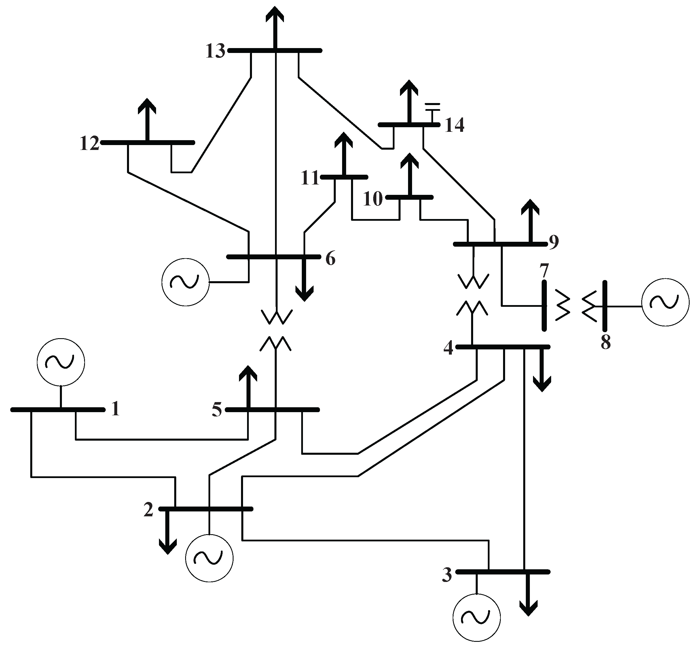
Figure 2.
Generation output and active demand for each dynamic load scenario, Case 1.
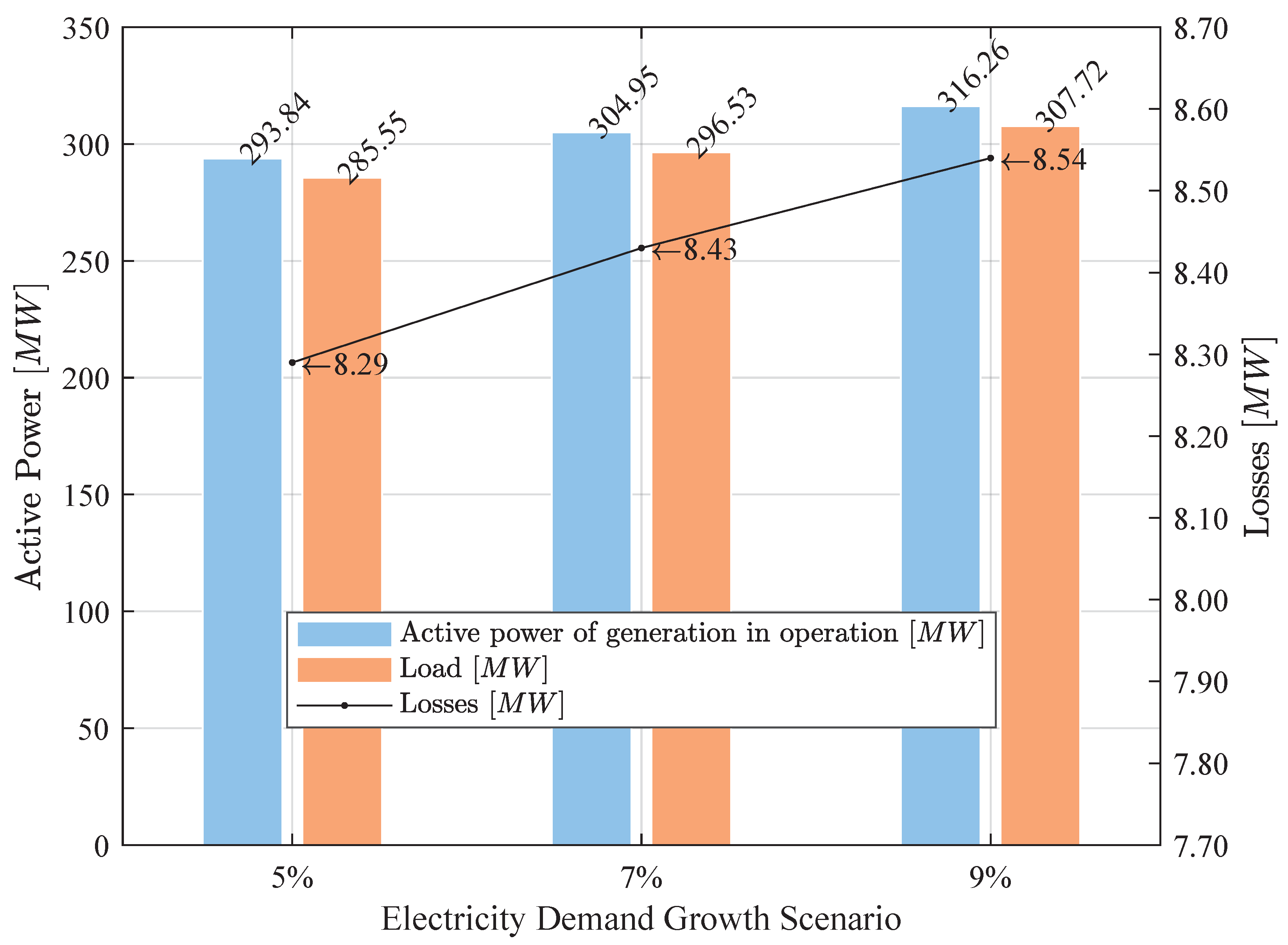
Figure 3.
Reactive generation output and demand for each dynamic load scenario, Case 1.
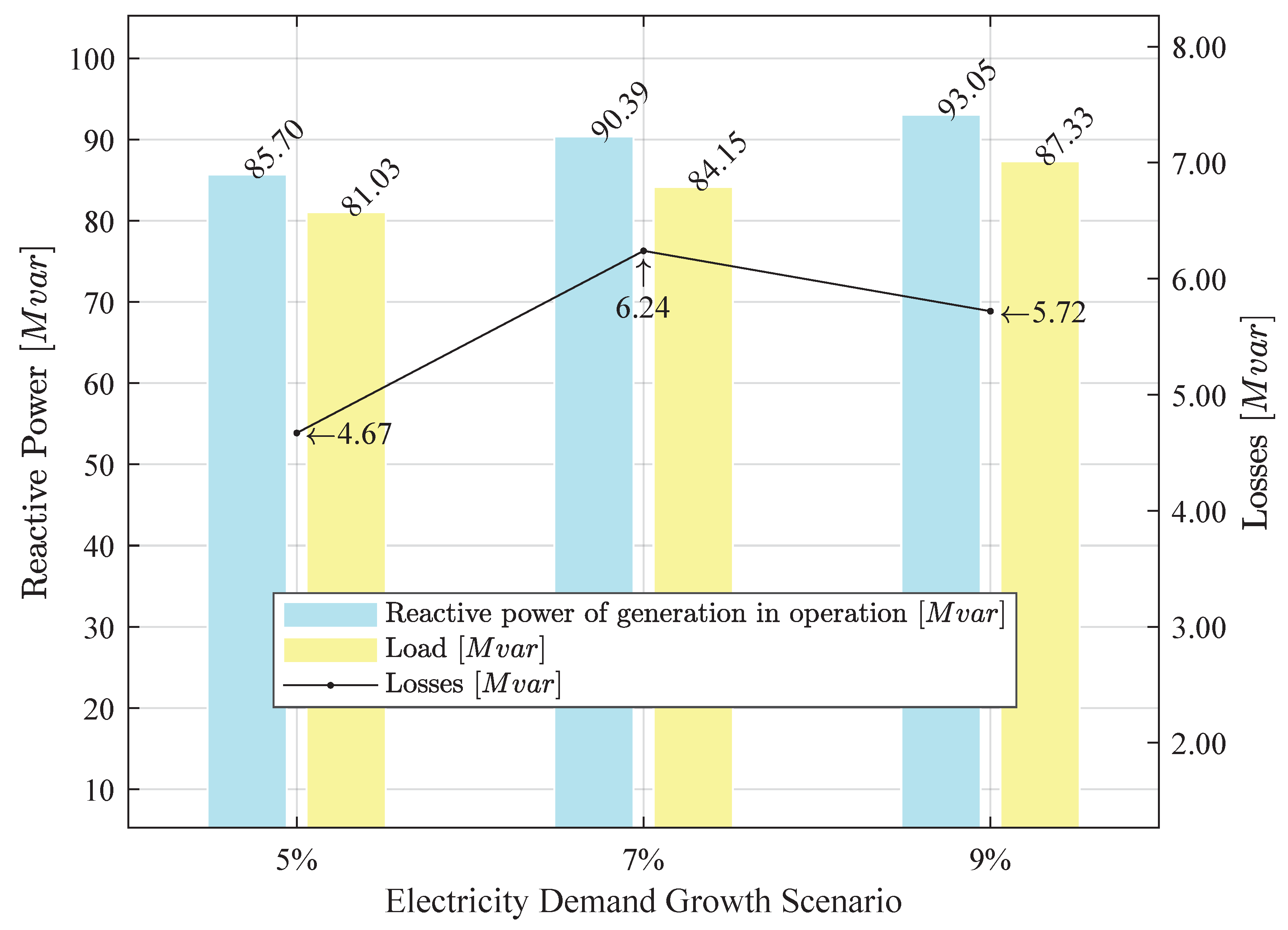
Figure 4.
Voltage profiles for each dynamic load scenario, Case 1.
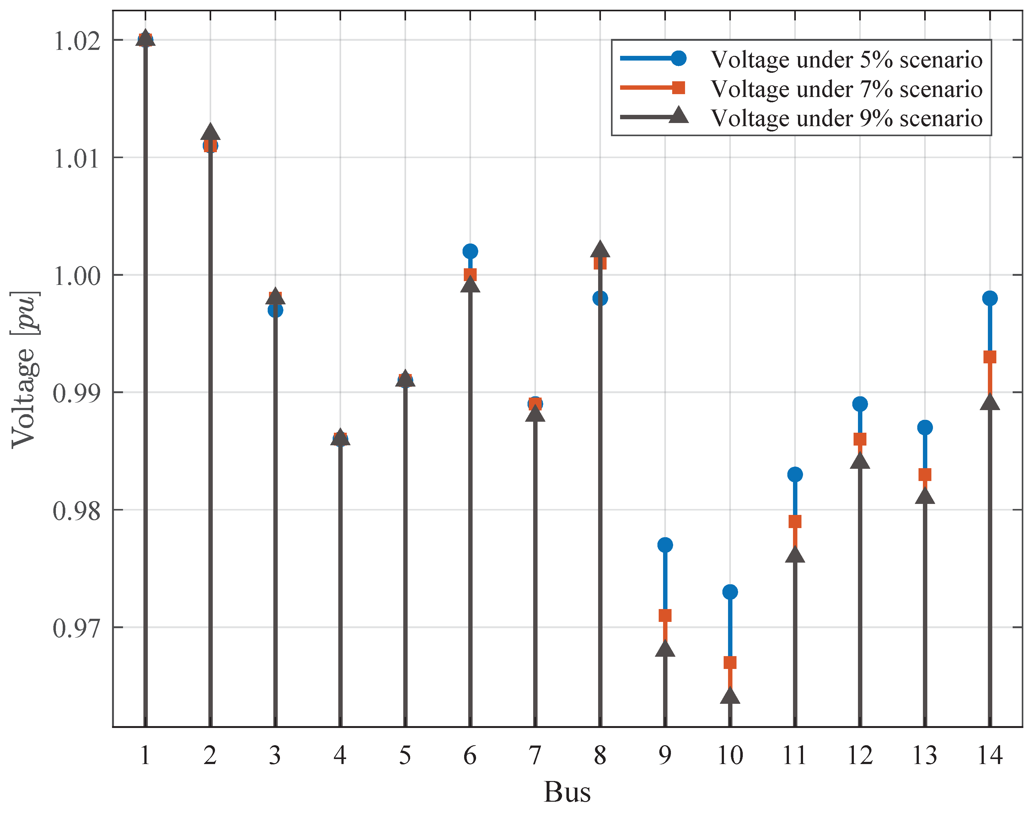
Figure 5.
Single-line diagram, Case 1: 5%, 7%, and 9%.
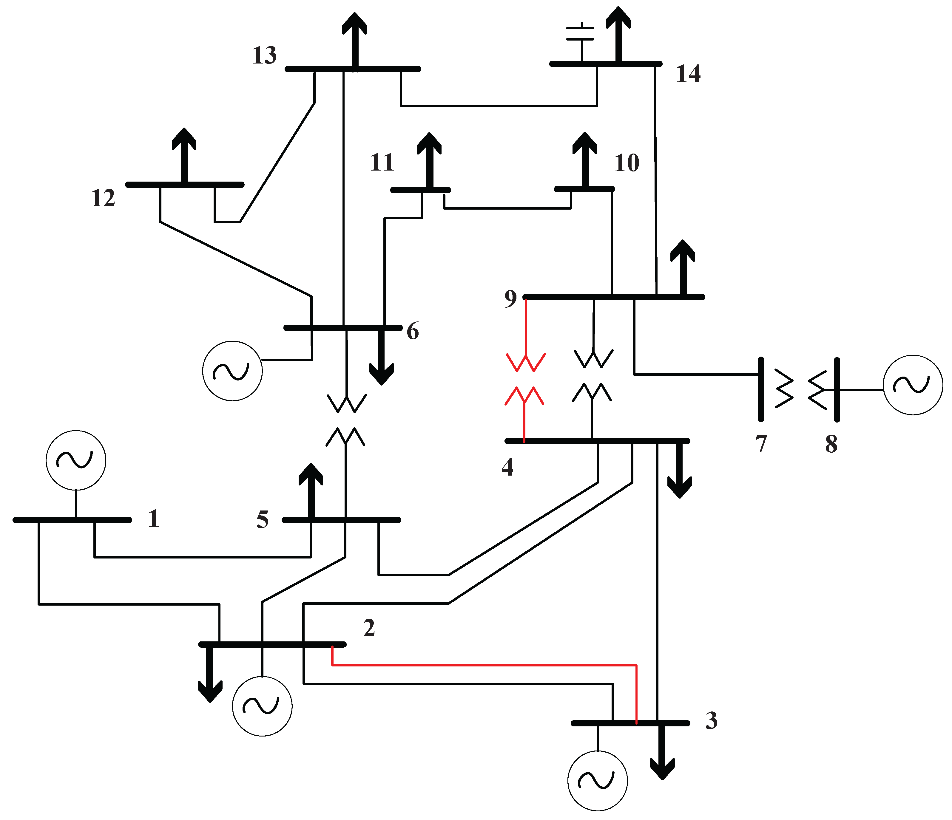
Figure 6.
Generation and active demand supplied for each dynamic load scenario, Case 2.
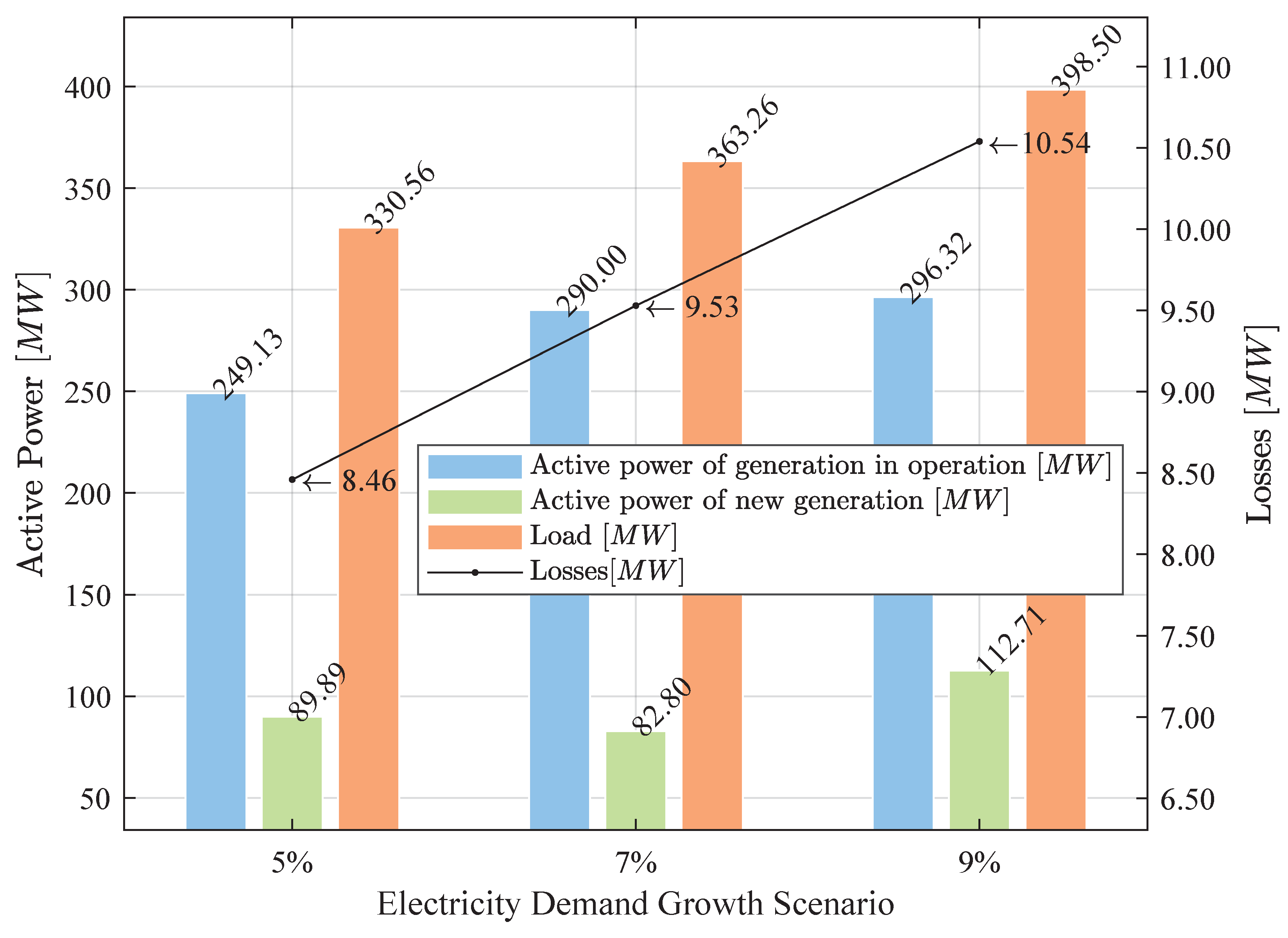
Figure 7.
Reactive generation and demand for each dynamic load scenario, Case 2.
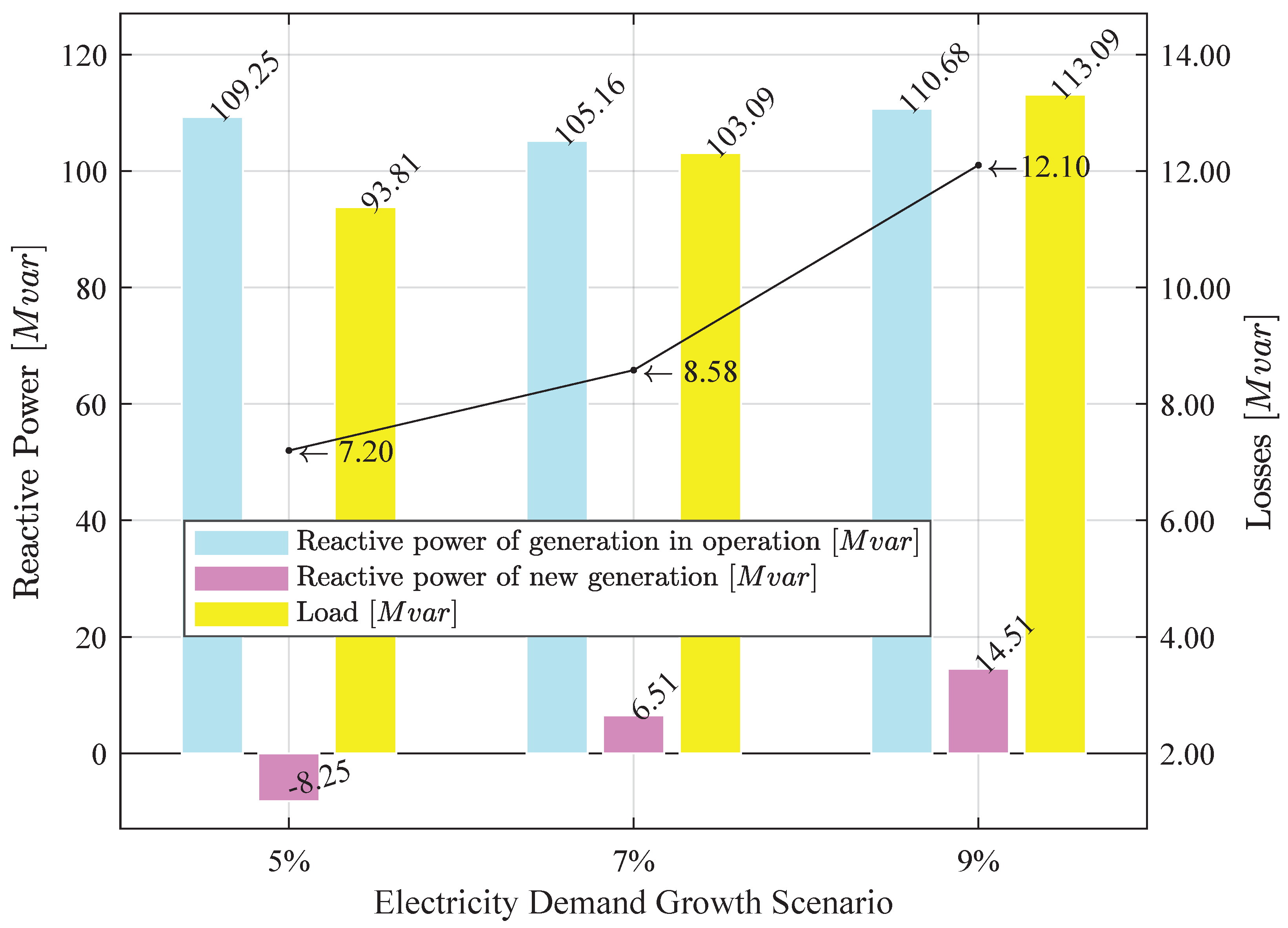
Figure 8.
Voltage profiles for each dynamic load scenario, Case 2.
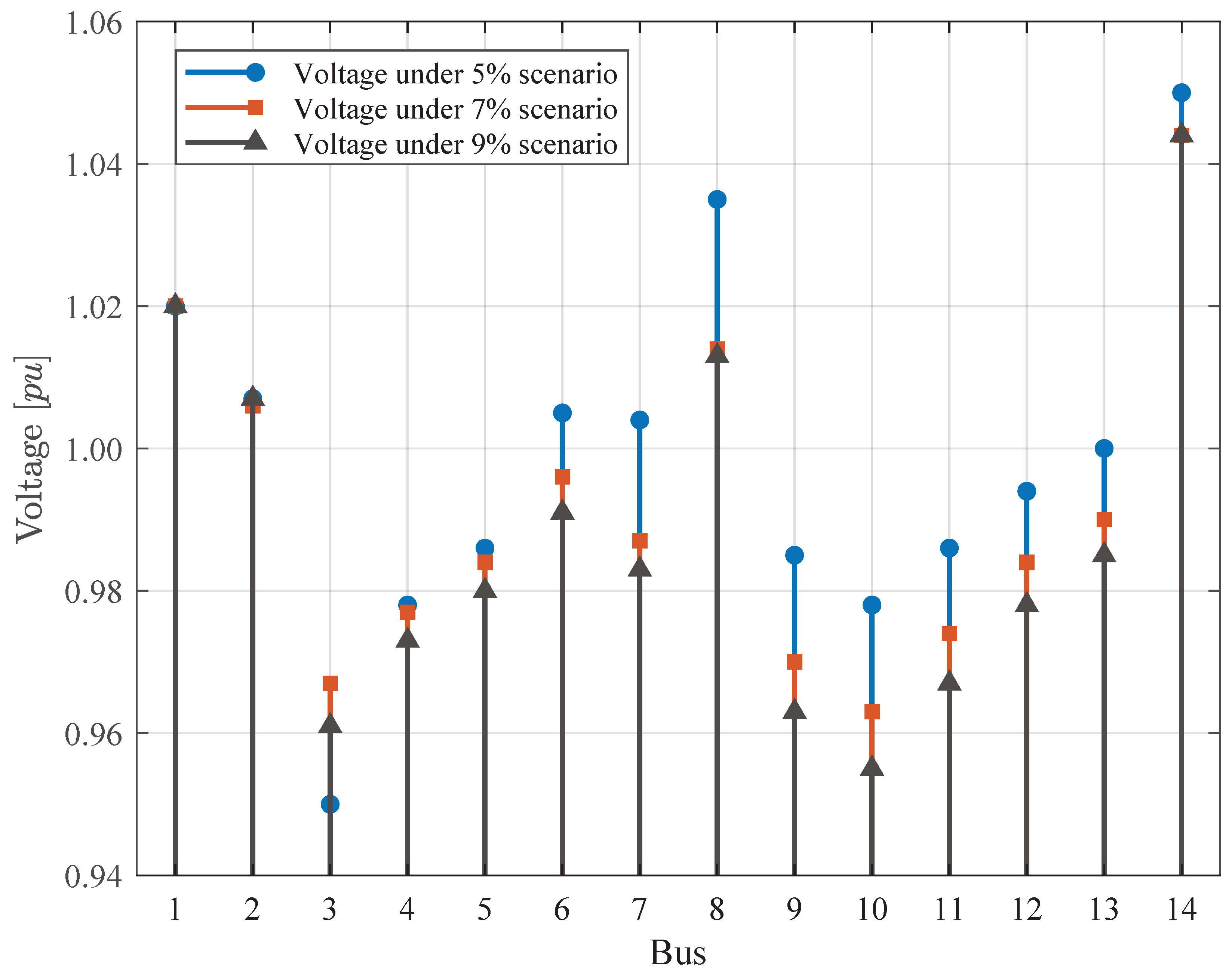
Figure 9.
One-line diagram, Case 2: 5%.
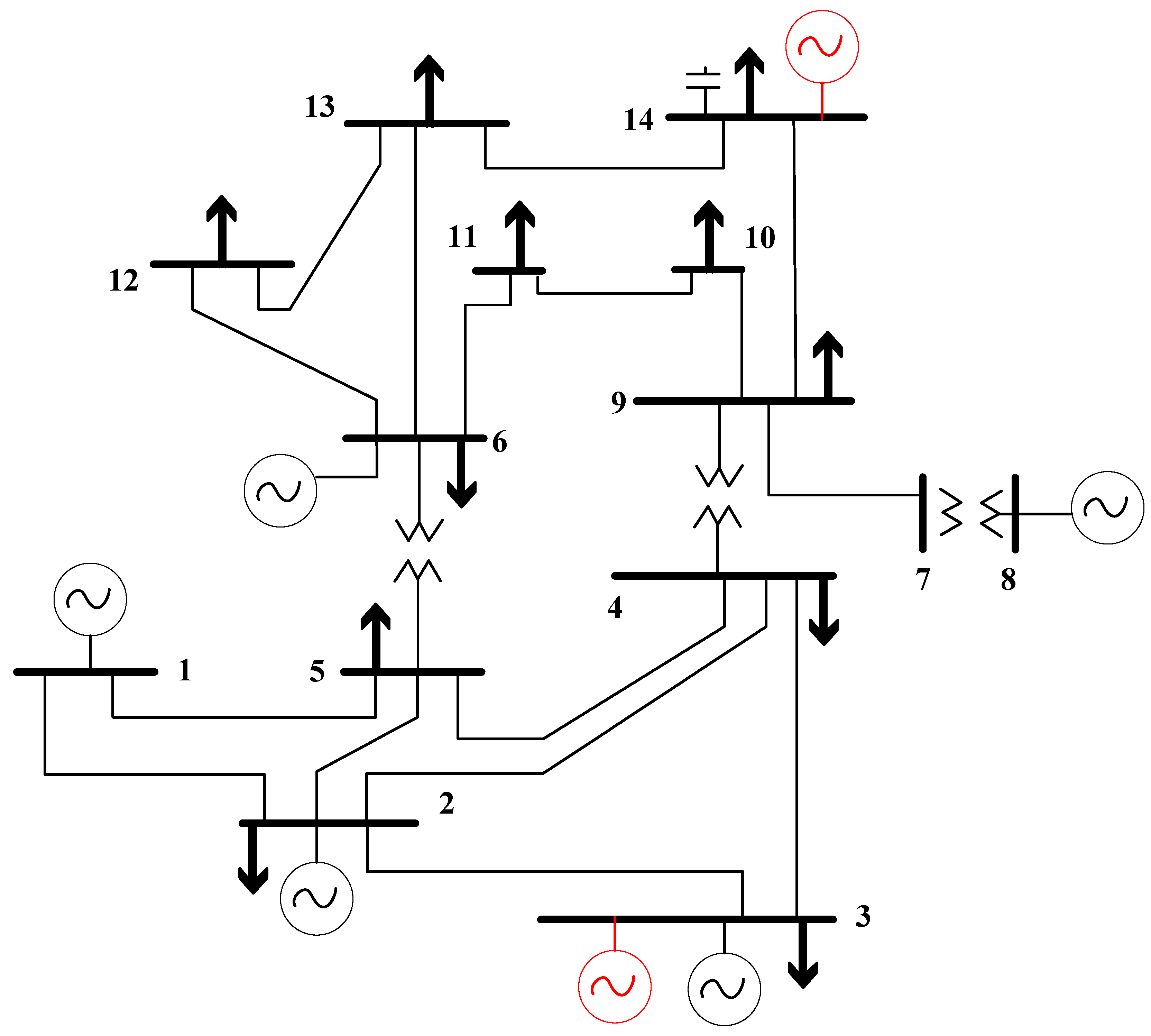
Figure 10.
One-line diagram, Case 2: 7 and 9%.
Representation 1.
Pseudocode of the optimization model.
| Simultaneous expansion of the generation park and the transmission system through mixed-integer nonlinear programming | |
| Step 1 | Acquisition of the power system data. |
| Step 2 | Determination of the factors associated with the expansion of the |
| generation and transmission stages: | |
| - Potential generators to be incorporated | |
| - Discount rate | |
| - Useful life | |
| - Demand growth rate | |
| - Cost of energy not supplied | |
| - Analysis period. | |
| Step 3 | Definition of variables |
| Continuous: | |
| Binary: | |
| Step 4 | Optimization model |
| Objective function | |
| Minimization of generation and transmission stage costs, including | |
| the cost of energy not supplied | |
| Constraints | |
| - Decision to implement new links | |
| - Power transfer limits of the links | |
| - Bidirectionality of decision variables for the | |
| new link | |
| - Nodal balance | |
| - Capacity of new generators | |
| - Generation output limits | |
| - Nodal voltage limits | |
| - Nodal angle limits. | |
| Step 5 | Application of the model to the case studies. |
| Step 6 | Analysis of results. |
| Step 7 | End. |
Table 1.
Parameters of the 14-bus network.
|
R [pu] |
X [pu] |
[pu] |
Limit [MVA] |
Cost [MMUSD] |
||
| 1 | 2 | 0.01938 | 0.05917 | 0.0528 | 120 | 66.63 |
| 1 | 5 | 0.05403 | 0.22304 | 0.0492 | 65 | 36.12 |
| 2 | 3 | 0.04699 | 0.19797 | 0.0438 | 36 | 20.00 |
| 2 | 4 | 0.05811 | 0.17632 | 0.0374 | 65 | 36.18 |
| 2 | 5 | 0.05695 | 0.17388 | 0.0340 | 50 | 27.76 |
| 3 | 4 | 0.06701 | 0.17103 | 0.0346 | 65 | 36.12 |
| 4 | 5 | 0.01335 | 0.04211 | 0.0128 | 45 | 25.01 |
| 4 | 7 | 0 | 0.55618 | 0 | 32 | 12.00 |
| 4 | 9 | 0 | 0.25202 | 0 | 45 | 14.00 |
| 5 | 6 | 0.09498 | 0.19890 | 0 | 18 | 26.99 |
| 6 | 11 | 0.12291 | 0.25581 | 0 | 32 | 47.96 |
| 6 | 12 | 0.06615 | 0.13027 | 0 | 32 | 48.10 |
| 6 | 13 | 0 | 0.17615 | 0 | 32 | 8.00 |
| 7 | 8 | 0.09711 | 0.11038 | 0 | 32 | 44.12 |
| 7 | 9 | 0.03181 | 0.08450 | 0 | 32 | 48.00 |
| 9 | 10 | 0.12711 | 0.27038 | 0 | 32 | 48.07 |
| 9 | 14 | 0.08205 | 0.19207 | 0 | 12 | 18.01 |
| 10 | 11 | 0.22092 | 0.19988 | 0 | 12 | 17.99 |
| 13 | 14 | 0.17093 | 0.34802 | 0 | 12 | 18.00 |
Table 2.
Bus data in the 14-bus network.
| Bus |
[MW] |
[Mvar] |
Area | Voltage [kV] |
| 1 | 0 | 0 | 1 | 138.0 |
| 2 | 21.7 | 12.7 | 1 | 138.0 |
| 3 | 94.2 | 19.0 | 1 | 138.0 |
| 4 | 47.8 | -3.9 | 1 | 138.0 |
| 5 | 7.6 | 1.6 | 1 | 138.0 |
| 6 | 11.2 | 7.5 | 1 | 138.0 |
| 7 | 0 | 0 | 2 | 69.0 |
| 8 | 0 | 0 | 3 | 13.8 |
| 9 | 29.5 | 16.6 | 2 | 69.0 |
| 10 | 9.0 | 5.8 | 2 | 69.0 |
| 11 | 3.5 | 1.8 | 2 | 69.0 |
| 12 | 6.1 | 1.6 | 2 | 69.0 |
| 13 | 13.5 | 5.8 | 2 | 69.0 |
| 14 | 14.9 | 5.0 | 2 | 69.0 |
Table 3.
Data of the generators in the 14-bus system.
| Bus |
[MW] |
[MW] |
Cost [USD/MWh] |
[Mvar] |
[Mvar] |
| 1 | 160 | 10 | 20 | 100 | -100 |
| 2 | 80 | 20 | 20 | 50 | -42 |
| 3 | 50 | 20 | 40 | 40 | 0 |
| 6 | 30 | 0 | 40 | 24 | -24 |
| 8 | 30 | 0 | 40 | 24 | -24 |
Table 4.
Technical data of the potential generators.
| Bus |
[MW] |
[MW] |
[Mvar] |
[Mvar] |
|
| 2 | 150 | 0 | 70 | -70 | |
| 6 | 100 | 0 | 60 | -60 | |
| 14 | 200 | 0 | 80 | -85 | |
| 3 | 100 | 0 | 60 | -60 | |
| 4 | 100 | 0 | 60 | -60 |
Table 5.
Economic data of the potential generators.
| Bus | Investment [USD/kW] |
Operating cost [USD/MWh] |
Lifetime Years |
||
| 2 | 1200 | 20 | 50 | 0.80 | |
| 6 | 600 | 50 | 20 | 0.94 | |
| 13 | 1000 | 30 | 50 | 0.82 | |
| 3 | 500 | 80 | 25 | 0.93 | |
| 4 | 350 | 120 | 25 | 0.96 |
Table 6.
Active power results by load scenario, Case 1.
| Load scenarios | |||
| Parameter [MW] | 5% | 7% | 9% |
| Active power from existing generation | 293.84 | 304.95 | 316.26 |
| New generation power | - | - | - |
| Load | 285.55 | 296.53 | 307.72 |
| Losses | 8.29 | 8.43 | 8.54 |
Table 7.
Reactive power results by load scenario, Case 1.
| Load scenarios | |||
| Parameter [Mvar] | 5% | 7% | 9% |
| Reactive power from existing generation | 85.700 | 90.394 | 93.046 |
| Reactive power from new generation | - | - | - |
| Load | 81.034 | 84.150 | 87.325 |
| Losses | 4.667 | 6.243 | 5.721 |
Table 8.
Activated transmission links by load scenario, Case 1.
| Load scenarios | |||
| Link | 5% | 7% | 9% |
| Link | ✓ | ✓ | ✓ |
| Link | ✓ | ✓ | ✓ |
Table 9.
Voltages by load scenario, Case 1.
| 5% | 7% | 9% | ||||
| Node | Voltage | Angle | Voltage | Angle | Voltage | Angle |
| [pu] | [deg] | [pu] | [deg] | [pu] | [deg] | |
| 1 | 1.020 | 0 | 1.020 | 0 | 1.020 | 0 |
| 2 | 1.011 | -3.53 | 1.011 | -3.53 | 1.012 | -3.54 |
| 3 | 0.997 | -5.32 | 0.998 | -7.54 | 0.998 | -7.56 |
| 4 | 0.986 | -5.68 | 0.986 | -5.69 | 0.986 | -5.66 |
| 5 | 0.991 | -7.21 | 0.991 | -7.23 | 0.991 | -7.18 |
| 6 | 1.002 | -13.05 | 1.000 | -13.66 | 0.999 | -13.23 |
| 7 | 0.989 | -13.20 | 0.989 | -14.46 | 0.988 | -14.23 |
| 8 | 0.998 | -12.58 | 1.001 | -13.42 | 1.002 | -13.04 |
| 9 | 0.977 | -13.29 | 0.971 | -14.72 | 0.968 | -14.57 |
| 10 | 0.973 | -13.61 | 0.967 | -14.91 | 0.964 | -14.73 |
| 11 | 0.983 | -13.49 | 0.979 | -14.45 | 0.976 | -14.15 |
| 12 | 0.989 | -14.18 | 0.986 | -14.89 | 0.984 | -14.52 |
| 13 | 0.987 | -14.43 | 0.983 | -15.20 | 0.981 | -14.85 |
| 14 | 0.998 | -16.08 | 0.993 | -17.29 | 0.989 | -17.12 |
Table 10.
Costs by load scenario, Case 1.
| Costs in million USD [MUSD] | |||
| Scenario | Network | Operation of | Total |
| 5% | 3.22 | 120.16 | 123.38 |
| 7% | 2.10 | 138.10 | 140.19 |
| 9% | 2.58 | 141.17 | 143.75 |
Table 11.
Active power results by load scenario, Case 2.
| Load Scenarios | |||
| Parameter [MW] | 5% | 7% | 9% |
| Active power from operating generation | 249.13 | 290.00 | 296.32 |
| Active power from new generation | 89.89 | 82.80 | 112.71 |
| Load | 330.56 | 363.26 | 398.50 |
| Losses | 8.46 | 9.53 | 10.54 |
Table 12.
Active power from new generation by load scenario, Case 2.
| Active Power [MW] | |||
| Load Scenarios | |||
| Location | 5% | 7% | 9% |
| Node 2 | - | 8.073 | 18.25 |
| Node 3 | 35.081 | 17.000 | 32.41 |
| Node 14 | 54.804 | 57.723 | 62.05 |
Table 13.
Reactive power results by load scenario – Case 2.
| Load Scenarios | |||
| Parameter [Mvar] | 5% | 7% | 9% |
| Reactive power from existing generation | 109.254 | 105.155 | 110.678 |
| Reactive power from new generation | -8.252 | 6.515 | 14.508 |
| Load | 93.807 | 103.088 | 113.089 |
| Losses | 7.195 | 8.582 | 12.097 |
Table 14.
Reactive power from new generation by load scenario, Case 2.
| Reactive Power [Mvar] | |||
| Load Scenarios | |||
| Location | 5% | 7% | 9% |
| Node 2 | - | 3.495 | 13.687 |
| Node 3 | -13.327 | -6.719 | -12.809 |
| Node 4 | 5.076 | 9.738 | 13.630 |
Table 15.
Network link activation by load scenario.
| Load Scenarios | |||
| Link | 5% | 7% | 9% |
| Link | - | ✓ | ✓ |
Table 16.
Voltages per load scenario, Case 2.
| 5% | 7% | 9% | ||||
| Node | Voltage | Angle | Voltage | Angle | Voltage | Angle |
| [pu] | [degree] | [pu] | [degree] | [pu] | [degree] | |
| 1 | 1.020 | 0 | 1.020 | 0 | 1.020 | 0 |
| 2 | 1.011 | -3.53 | 1.011 | -3.53 | 1.012 | -3.54 |
| 3 | 0.997 | -5.32 | 0.998 | -7.54 | 0.998 | -7.56 |
| 4 | 0.986 | -5.68 | 0.986 | -5.69 | 0.986 | -5.66 |
| 5 | 0.991 | -7.21 | 0.991 | -7.23 | 0.991 | -7.18 |
| 6 | 1.002 | -13.05 | 1 | -13.66 | 0.999 | -13.23 |
| 7 | 0.989 | -13.20 | 0.989 | -14.46 | 0.988 | -14.23 |
| 8 | 0.998 | -12.58 | 1.001 | -13.42 | 1.002 | -13.04 |
| 9 | 0.977 | -13.29 | 0.971 | -14.72 | 0.968 | -14.57 |
| 10 | 0.973 | -13.61 | 0.967 | -14.91 | 0.964 | -14.73 |
| 11 | 0.983 | -13.49 | 0.979 | -14.45 | 0.976 | -14.15 |
| 12 | 0.989 | -14.18 | 0.986 | -14.89 | 0.984 | -14.52 |
| 13 | 0.987 | -14.43 | 0.983 | -15.20 | 0.981 | -14.85 |
| 14 | 0.998 | -16.08 | 0.993 | -17.29 | 0.989 | -17.12 |
Table 17.
Costs per load scenario.
| Costs in million US dollars [MUSD] | |||
| Scenario | Network | Operation of | Operation of |
| 5% | - | 262.04 | 194.94 |
| 7% | 1.61 | 297.84 | 142.49 |
| 9% | 1.61 | 308.92 | 211.09 |
| Scenario | Investment in | Total | |
| 5% | 7.46 | 464.44 | |
| 7% | 7.74 | 449.67 | |
| 9% | 10.25 | 531.88 | |
Disclaimer/Publisher’s Note: The statements, opinions and data contained in all publications are solely those of the individual author(s) and contributor(s) and not of MDPI and/or the editor(s). MDPI and/or the editor(s) disclaim responsibility for any injury to people or property resulting from any ideas, methods, instructions or products referred to in the content. |
© 2025 by the authors. Licensee MDPI, Basel, Switzerland. This article is an open access article distributed under the terms and conditions of the Creative Commons Attribution (CC BY) license (http://creativecommons.org/licenses/by/4.0/).
Copyright: This open access article is published under a Creative Commons CC BY 4.0 license, which permit the free download, distribution, and reuse, provided that the author and preprint are cited in any reuse.


