
Submitted:
20 March 2025
Posted:
21 March 2025
You are already at the latest version
Abstract
This paper proposes a methodology for the co-expansion planning of transmission lines and energy storage devices, considering unit commitment constraints and uncertainties in load demand and wind generation. The problem is formulated as a mixed-integer nonlinear program (MINLP) and solved using a decomposition-based approach that combines a genetic algorithm with mixed-integer linear programming (MILP). Uncertainties are modeled through representative day scenarios obtained via clustering. The proposed methodology is validated on a modified IEEE 24-bus system. Results show that co-planning reduces wind curtailment, fuel costs, and total investment costs compared to transmission-only expansion.
Keywords:
Co-Expansion Planning of Transmission Lines and Energy Storage Devices
; Unit Commitment
; Renewable Energy
; Energy Storage System
1. Introduction
Transmission Network Expansion Planning (TNEP) is a fundamental aspect of power system planning that determines where, when, and how many new transmission lines should be added to the network. The objective is to minimize investment and operational costs while satisfying technical, economic, and reliability constraints. TNEP must ensure adequate transmission capacity to deliver secure and reliable electric power to the load centers along the planning horizon.
The increasing integration of non-dispatchable renewable energy sources, such as wind and solar power, coupled with the urgency to reduce greenhouse gas emissions, has intensified efforts to mitigate renewable energy curtailment caused by transmission congestion. A viable solution is the deployment of energy storage systems (ESSs), which store excess energy during periods of high renewable generation and low demand, then discharge it when renewable output declines and demand rises. In addition, ESSs improve network operation by providing voltage control, energy flow management, and system restoration, improving overall grid stability and efficiency.
Co-expansion planning of transmission lines and energy storage devices (CETES) has gained significant attention in recent years due to its economic and technical benefits. This approach optimizes renewable energy utilization, alleviates transmission congestion, and reduces the need for additional transmission investments. However, despite its advantages, few studies incorporate Unit Commitment (UC) constraints into this framework.
The UC problem determines the optimal scheduling of generation units to minimize operational costs while satisfying system constraints. The increasing penetration of intermittent renewable sources introduces uncertainties that complicate UC decisions, requiring frequent adjustments in thermal generation. ESSs mitigate these challenges by smoothing power fluctuations, reducing the reliance on costly and polluting spinning reserves, and improving system reliability.
1.1. Literature Review
Co-expansion planning of transmission lines and energy storage devices (CETES) has been the focus of recent research efforts. Table 1 summarizes the main characteristics of recent publications that propose methodologies to solve CETES. Table 1 provides a structured summary of the key characteristics of recent studies on CETES, highlighting their methodological approaches, network modeling assumptions, investment variable formulations, and solution techniques. The articles are arranged in chronological order to illustrate the evolution of research in this field.
In the reviewed models, two types of investment formulations for energy storage devices were identified: continuous (C) and binary (B). Binary formulations allow the allocation of storage devices with predefined power and energy capacity values, including integer-variable formulations. In contrast, continuous formulations optimize the power and energy capacities of the installed storage devices.
Regarding the planning horizon, CETES can be modeled in two ways: static (S) or dynamic (D), also referred to as multistage. Static models assume that all investments occur at the beginning of the period and are based on electricity demand at the end of the planning horizon, without considering construction timelines. In contrast, dynamic CETES divides the planning horizon into multiple stages, incorporating time constraints and interdependencies among investment decisions.
The reviewed works considered four energy storage technologies: Generic Energy Storage Systems (GESS), Battery Energy Storage Systems (BESS), Compressed Air Energy Storage (CAES), and Pumped Hydro Energy Storage (PHES). The term GESS is used for studies that consider energy storage systems without specifying a particular technology.
Most studies employ a DC power flow model without losses, a widely used linear formulation in CETES modeling. Furthermore, CETES solution methods primarily rely on mixed-integer linear programming (MILP) formulations, decomposition techniques, and column-and-constraint generation (CCG).
Among the evaluated papers, only one incorporated Unit Commitment (UC) constraints, highlighting an opportunity for further advancements in co-planning formulations of transmission and storage devices.
Several studies have modeled CETES as a MILP problem. In [1,2], static CETES is analyzed without chronological scenarios, limiting accuracy by neglecting the dynamic behavior of demand and renewable energy sources. While [2] incorporates transmission losses, [1] assumes a lossless network. Reference [14] models static CETES with energy balance constraints and the N-1 security criterion, including investments in CAES and representative seasonal demand profiles. However, it does not account for renewable generation uncertainties or unit commitment constraints.
Dynamic CETES has been widely investigated using MILP formulations. [3] introduces an eight-year planning horizon divided into two four-year stages, incorporating wind generation but omitting uncertainties. [6] applies Nested Benders decomposition, considering long-term uncertainties and investments in storage and transmission lines with different construction times. [12] employs Benders decomposition for a multistage CETES problem, integrating the N-1 security criterion and evaluating storage performance under contingencies.
To improve computational efficiency, several works adopt decomposition techniques. The work [4] applies Benders decomposition, modeling storage investment as a continuous variable, diverging from previous discrete approaches. Reference [15] proposes a block-based multicut Benders decomposition to reduce simulation time and enhance expansion planning. [13] integrates thyristor-controlled series compensators within a linearized AC optimal power flow MILP formulation, making the model applicable to reactive power studies.
Robust and hybrid optimization methods have also been explored. In [9] formulates a three-level adaptive robust CETES model, addressing long-term uncertainties through robust sets and short-term variations via representative days, though it does not include unit commitment. [10] develops a hybrid stochastic-robust approach with continuous-time modeling to determine power scheduling and ramping activation, enabling fast sub-hourly adjustments to accommodate wind uncertainty and load variations. Reference [11] applies a robust co-planning strategy via the column-and-constraint generation algorithm, though the binary representation of storage charging/discharging increases computational complexity.
Market-driven CETES models have also been studied. The work [7] incorporates BESS with capacity degradation and system lifetime effects, optimizing storage operation across price fluctuations based on representative daily scenarios. In [8], the authors proposes a three-level CETES model, where the upper level maximizes storage profitability, the middle level optimizes transmission expansion, and the lower level simulates market clearing. The problem is reformulated into a bi-level structure and solved via CCG.
Among the reviewed studies, [5] is the only one explicitly incorporating a unit commitment model for thermal units. It includes wind and load scenarios over a 25-year horizon while accounting for transmission expansion delays and battery degradation. However, its UC model is overly simplistic, using a single binary variable to indicate generator status while disregarding minimum up/down times, startup/shutdown ramps.
2. Contributions
Building upon insights from prior literature, this paper introduces a methodology for addressing the co-expansion planning of transmission lines and energy storage devices, accounting for uncertainties in both load demand and wind generation through probabilistic representative days. Furthermore, constraints on the unit commitment of thermal generation units are incorporated into the model, an aspect that has been minimally explored in the literature.
- Formulating a stochastic optimization model for the co-expansion planning of transmission lines and energy storage devices.
- Proposing a solution strategy to address the problem, which involves decomposing the problem into a master problem and a subproblem.
- Presenting a methodology based on genetic algorithms and classical optimization techniques to solve the proposed formulation.
3. Problem Formulation
The proposed co-expansion planning of transmission lines and energy storage devices (CETES) is formulated as a bilevel stochastic mixed-integer nonlinear optimization model. This formulation incorporates static planning for the long-term horizon and adopts the DC network representation. The unit commitment model follows the approach proposed in [16], which requires fewer binary variables and constraints compared to other formulations, such as [17,18,19], significantly reducing computational complexity. This formulation effectively handles intertemporal constraints, including ramping limits and minimum up and down times. Uncertainties in wind generation and load profiles are addressed using representative daily scenarios. Each scenario is assigned a probability weight that reflects its expected occurrence over the year. The complete optimization model is presented in (1)–(32).
3.1. Objective Function
The objective function minimizes the total cost (C), which consists of four components. The first term represents the annualized investment cost in transmission lines (). The second and third terms correspond to the annualized investment cost in energy storage devices. Since the investment cost in energy storage depends on both the energy and power ratings of the unit, represents for the energy component, while represents the power component of the cost. Finally, the fourth term captures the operational cost over a one-year horizon, considering representative daily scenarios. This cost includes the generation cost of thermal units, the operational cost of storage systems, and the curtailment cost of wind generation. The mathematical formulation of the objective function is presented in (1)–(5).
3.2. Constraints
The constraints (6) and (7) enforce the investment in transmission line and energy storage divce, respectively.
The constraints related to power flow are presented in (8)–(14). Constraint (8) ensures power balance at each bus. Constraints (9) and (10) model the power flow through existing and candidate transmission lines, respectively. Constraints (11) and (12) enforce power flow limits on existing and candidate lines, respectively. Constraint (13) defines the upper and lower limits for the bus angles, while the constraint (14) sets the angle of the reference bus to zero.
The constraints related to the operation of thermal generator units are presented in (15)–(25). These constraints represent the unit commitment model proposed in [16]. Constraint (15) defines the generation limits for each unit, ensuring that the power output remains within the minimum and maximum allowed values. Constraint (16) limits the maximum available power output of each unit, considering its on/off status. Constraint (17) enforces ramp-up and startup ramp limits. Constraint (18) enforces shutdown ramp limits. Constraint (19) imposes ramp-down limits. Constraint (20) ensures that units initially online remain online for the required minimum up-time. Constraint (21) ensures that once a unit is started, it remains online for the specified minimum up-time. Constraint (22) ensures that units started near the end of the time horizon remain online until the end. Constraint (23) ensures that units initially offline remain offline for the required minimum down-time. Constraint (24) ensures that once a unit is shut down, it remains offline for the specified minimum down-time. Constraint (25) ensures that units shut down near the end of the time horizon remain offline until the end.
The constraints related to energy storage devices are presented in (26)–(32). Constraints (26) and (27) limit the state of charge (SOC) of the existing and candidate storage devices, respectively. Constraints (28) and (29) limit the discharge power of existing and candidate storage devices, respectively. Constraints (30) and (31) limit the charge power of existing and candidate storage devices, respectively. Constraint (32) represents the energy balance of the storage devices, updating the SOC based on charging and discharging.
The constraint (35) limits the curtailment of the wind, ensuring that the curtailed power does not exceed the available wind generation.
4. Solution Strategy
To address the mixed-integer nonlinear problem, this work proposes a decomposition strategy that separates it into an investment master problem and an operational subproblem.
The investment master problem determines the optimal investment decisions by defining the integer investment variables for transmission lines and energy storage devices .
The operational subproblem evaluates the operational cost of the system () in all scenarios over a one-year horizon. This cost is then fed back into the investment master problem to iteratively refine investment decisions. The operational subproblem solves the network-constrained unit commitment for each scenario, treating the investments determined by the master problem as implemented. Specifically, transmission lines and storage devices with positive investment values ( or ) are incorporated into the sets of existing transmission lines () and storage systems ().
This decomposition eliminates the nonlinearity of the original problem, allowing an iterative solution process between the investment master problem and the operational subproblem. The investment problem is solved using a genetic algorithm-based optimization approach, while the operational subproblem is addressed with commercial MILP solvers. Figure 1 illustrates the process.
4.1. Investment Master Problem
The genetic algorithm used in this study employs four main operators: selection, crossover, mutation, and elitism.
Each chromosome (individual) consists of two independent segments: one for transmission line investments and another for storage system investments. Figure 2 illustrates a chromosome representation for a fictitious system with five candidate branches for transmission expansion and four candidate buses for the installation of energy storage. In this example, the chromosome specifies the construction of one transmission line on the first candidate branch, two lines on the third, and three lines on the fourth. Similarly, it indicates investments in five storage units at the first candidate bus and three at the second.
To maintain structural integrity, crossover and mutation operations are applied separately within each segment (transmission line investment or energy storage investment). This prevents infeasible solutions caused by swapping genes between unrelated components, since the upper limits and may differ depending on the system under analysis.
The crossover process is modified to occur exclusively within each segment. This prevents transmission line investments from being swapped with storage investments, preserving chromosome integrity, and eliminating the risk of infeasible solutions.
Mutation operator adjustments are made so that random alterations affect only one category at a time (transmission, storage, or both). This ensures that mutations adhere to system constraints, preventing structural inconsistencies.
The fitness value of each chromosome is computed after solving the operational subproblem. It corresponds to the sum of the four cost components in the original objective function (1) plus a penalty cost . A lower fitness value indicates a better performing chromosome relative to others.
The penalty cost is applied when the operational subproblem is infeasible for any scenario analyzed. To strongly discourage insufficient investment solutions, a high penalty value is used.
4.2. Operational Subproblem
The operational subproblem receives investment decisions from the investment master problem, specifically the integer investment variables for transmission lines () and energy storage devices (). Transmission lines and storage devices with positive investment values ( or ) are incorporated into the sets of existing transmission lines () and storage systems ().
Based on these decisions, the operational subproblem is formulated as a stochastic network-constrained unit commitment model, represented as a mixed-integer linear optimization problem. The objective is to minimize the annual operational cost while accounting for uncertainties in wind generation and electricity demand. A set of representative daily scenarios is considered, where each scenario is assigned a probability weight , reflecting its probability of occurrence over the year.
5. Simulations
This section presents the results obtained using the proposed methodology on a modified IEEE-RTS 24-bus test system [20]. The system comprises 24 buses and 41 candidate branches for expansion. Each branch can accommodate up to three transmission lines. The investment costs for the candidate lines of 230 kV and 132 kV are $120,000.0/km and $70,000.0/km, respectively [20].
The load profile and technical data for thermal generator units are taken from [21]. The original system data presented in [20] and [21] are not suitable for long-term planning. To accommodate a long-term planning approach, the capacities of all existing transmission lines are reduced to one-third of their original values, following [2]. In addition, the maximum thermal generator capacity and up-ramp limit are doubled.
The system includes three wind farms located at buses 20, 21, and 23, with maximum generation capacities of 900.0 MW, 600.0 MW, and 300.0 MW, respectively. Following [22], the generation cost of these wind farms is set to zero. The curtailment cost of wind generation is adopted as 80 $/MW, as used in [23].
Energy storage investments are considered at buses 5, 6, 8, 10, 11, and 14, following [15]. Each bus can accommodate up to five storage units, with each unit having a power capacity of 100 MW and an energy capacity of 500 MWh. The subsidized costs are set at $500.0/kW (power) and $20.0/kWh (energy), as used in [8]. The charging and discharge efficiencies of the energy storage device are 95%. Investment costs are annualized using an interest rate 5%, with assumed lifetimes of 60 years for transmission lines [8,15] and 20 years for storage devices [15]. The maximum number of energy storage devices that can be invested at each bus is five.
The study analyzes five representative daily scenarios to capture hourly variations in demand and wind generation at the three wind farms. These scenarios are derived from historical load and wind generation data [24]. The k-means clustering technique is applied to group the data and assign weighted probabilities to each scenario. The complete system data are available in [?].
Two case studies are investigated:
- Case A: Investments in transmission line
- Case B: Investments in transmission line and energy storage device
The parameters of the genetic algorithm are presented in Table 2. These parameters were defined empirically. For all cases, the convergence criterion is the maximum number of iterations. Ten simulations were conducted for each case defined below. All simulations were performed on a 2.7 GHz Intel® Core i7 processor, with the codes implemented in MATLAB® software version R2015a.
5.1. Results
Table 3 presents the best investment solution found for each case.
For Case A, the optimal solution includes a transmission line investment cost of 1,494.0 M$, involving the construction of one line between buses 2–6, 3–9, 4–9, 6–10, 7–8, 9–12, 12–23, 14–16, 15–16, 16–17, 18–21, 20–23, and 14–23. Additionally, two transmission lines are constructed between buses 1–5, 9–11, 11–14, 12–13, 17–22, and 1–8, while three lines are added between buses 6–7. The corresponding annual operational cost is 42,702.86 M$.
For Case B, the optimal solution involves a transmission line investment cost of 1,193.00 M$ and an energy storage investment of 136.00 M$. The transmission expansion plan suggests constructing new lines between buses 2–6, 3–9, 3–24, 4–9, 5–10, 6–10, 8–9, 9–11, 10–11, 11–14, 12–23, 14–16, 15–21, 15–24, 16–17, 17–18, 17–22, 20–23, and 13–14, along with the addition of two transmission lines between buses 1–5, 7–8, 1–8, and 14–23.
The investment in energy storage includes the installation of one storage unit at bus 5, one unit at bus 6, two storage units at buses 11 and 14, and three units at bus 14. This combined investment in transmission lines and energy storage results in an annual operating cost of 81,60 M$.
It is evident that Case B presents a more cost-effective transmission expansion plan compared to Case A, with a cost reduction of 20.15%. The total expansion cost in Case B, including both transmission line and energy storage investments 1,274.6 M$, remains 14.69% lower than the transmission expansion cost in Case A. Additionally, the annual operating cost of Case B is 26.19% lower than that of Case A. These results highlight the economic benefits of considering the co-expansion planning of transmission lines and energy storage devices.
Table 4 summarizes the cumulative stochastic thermal generation, stochastic charge and discharge energy, stochastic charge and discharge power of storage systems, and stochastic wind generation curtailment for the best solutions obtained in each case, considering the sum across all five scenarios. The cumulative total thermal generation and wind curtailment are lower in Case B than in Case A, with a difference of 87.25 MWh. Over a year, this reduction amounts to 31,846.25 MWh.
This reduction is primarily due to the presence of energy storage systems, which decrease reliance on thermal generation by enhancing operational flexibility and enabling a more cost-effective dispatch of thermal units while adhering to unit commitment constraints. Furthermore, storage systems mitigate wind curtailment by storing surplus wind energy and discharging it when it is most economically beneficial to the system. As a result, Case B achieves a 91.99% reduction in curtailed wind energy compared to Case A.
Table 5 and Table 6 present the optimal dispatch of the thermal generator units for each hour of the first scenario, corresponding to the best solution found for Case A and Case B, respectively. These tables demonstrate that the model complies with unit commitment constraints, thus validating the effectiveness of the proposed methodology.
Figure 3 and Figure 4 present the charge and discharge output for the first scenario of the energy storage devices invested in Case B. It can be observed that the storage systems follow a charging pattern during the early hours of the day (00:00 – 05:00) and the late evening (20:00 – 23:00), periods when the demand is lower. In contrast, the discharge occurs primarily in the afternoon (12:00 – 19:00), aligning with the period of higher load demand.
6. Conclusions
This paper presents a methodology for co-expansion planning of transmission lines and energy storage devices, considering uncertainties in load demand and wind generation through probabilistic representative days. In addition, the model integrates unit commitment constraints for thermal generation units, enhancing the realism of the planning process.
To solve the proposed formulation, the optimization methodology decomposes the problem into a master problem and a subproblem, utilizing genetic algorithms and classical optimization techniques to efficiently address the mixed-integer linear problem."
The results highlight the interdependence between transmission expansion and energy storage investments, as well as their impact on market indices. Furthermore, the findings indicate that co-planning transmission lines and energy storage devices leads to greater economic efficiency, reducing both investment and operational costs compared to planning transmission expansion alone.
Author Contributions
The authors contributed equally to this work.
Funding
Please add: “This research received no external funding” or “This research was funded by NAME OF FUNDER grant number XXX.” and and “The APC was funded by XXX”. Check carefully that the details given are accurate and use the standard spelling of funding agency names at https://search.crossref.org/funding, any errors may affect your future funding.
Acknowledgments
The authors gratefully acknowledge the Brazilian agency for the financial support in part of the Brazilian Federal Agency for the Support and Evaluation of Graduate Education (CAPES), the National Research Council (CNPq), the Brazilian Institute of Science and Technology (INERGE) and the State of Minas Gerais Research Foundation (FAPEMIG). The authors also express gratitude for the educational support of the Federal University of Juiz de Fora (UFJF).
Conflicts of Interest
The authors declare no conflicts of interest.
References
- Hu, Z.; Zhang, F.; Li, B. Transmission expansion planning considering the deployment of energy storage systems. In Proceedings of the 2012 IEEE Power and Energy Society General Meeting. IEEE, 2012; pp. 1–6. [Google Scholar]
- Zhang, F.; Hu, Z.; Song, Y. Mixed-integer linear model for transmission expansion planning with line losses and energy storage systems. IET Generation, Transmission & Distribution 2013, 7, 919–928. [Google Scholar]
- Hedayati, M.; Zhang, J.; Hedman, K.W. Joint transmission expansion planning and energy storage placement in smart grid towards efficient integration of renewable energy. In Proceedings of the 2014 IEEE PES T&D Conference and Exposition. IEEE, 2014; pp. 1–5. [Google Scholar]
- MacRae, C.; Ernst, A.; Ozlen, M. A Benders decomposition approach to transmission expansion planning considering energy storage. Energy 2016, 112, 795–803. [Google Scholar] [CrossRef]
- Qiu, T.; Xu, B.; Wang, Y.; Dvorkin, Y.; Kirschen, D.S. Stochastic multistage coplanning of transmission expansion and energy storage. IEEE Transactions on Power Systems 2016, 32, 643–651. [Google Scholar] [CrossRef]
- Falugi, P.; Konstantelos, I.; Strbac, G. Planning with multiple transmission and storage investment options under uncertainty: A nested decomposition approach. IEEE Transactions on Power Systems 2017, 33, 3559–3572. [Google Scholar] [CrossRef]
- Aguado, J.; de La Torre, S.; Triviño, A. Battery energy storage systems in transmission network expansion planning. Electric Power Systems Research 2017, 145, 63–72. [Google Scholar] [CrossRef]
- Dvorkin, Y.; Fernández-Blanco, R.; Wang, Y.; Xu, B.; Kirschen, D.S.; Pandžić, H.; Watson, J.P.; Silva-Monroy, C.A. Co-planning of investments in transmission and merchant energy storage. IEEE Transactions on Power Systems 2017, 33, 245–256. [Google Scholar] [CrossRef]
- Zhang, X.; Conejo, A.J. Coordinated investment in transmission and storage systems representing long-and short-term uncertainty. IEEE Transactions on Power Systems 2018, 33, 7143–7151. [Google Scholar] [CrossRef]
- Nikoobakht, A.; Aghaei, J. Integrated transmission and storage systems investment planning hosting wind power generation: Continuous-time hybrid stochastic/robust optimisation. IET Generation, Transmission & Distribution 2019, 13, 4870–4879. [Google Scholar]
- Wang, S.; Geng, G.; Jiang, Q. Robust co-planning of energy storage and transmission line with mixed integer recourse. IEEE Transactions on Power Systems 2019, 34, 4728–4738. [Google Scholar] [CrossRef]
- Gan, W.; Ai, X.; Fang, J.; Yan, M.; Yao, W.; Zuo, W.; Wen, J. Security constrained co-planning of transmission expansion and energy storage. Applied energy 2019, 239, 383–394. [Google Scholar] [CrossRef]
- Luburić, Z.; Pandžić, H.; Carrión, M. Transmission expansion planning model considering battery energy storage, TCSC and lines using AC OPF. IEEE access 2020, 8, 203429–203439. [Google Scholar] [CrossRef]
- Mazaheri, H.; Abbaspour, A.; Fotuhi-Firuzabad, M.; Moeini-Aghtaie, M.; Farzin, H.; Wang, F.; Dehghanian, P. An online method for MILP co-planning model of large-scale transmission expansion planning and energy storage systems considering N-1 criterion. IET Generation, Transmission & Distribution 2021, 15, 664–677. [Google Scholar]
- de Oliveira, E.J.; de Paula, A.N.; de Oliveira, L.W.; Honório, L.d.M.; et al. Block-Based Multicut Benders Decomposition Algorithm for Transmission and Energy Storage Co-Planning. International Transactions on Electrical Energy Systems 2022, 2022. [Google Scholar] [CrossRef]
- Carrión, M.; Arroyo, J.M. A computationally efficient mixed-integer linear formulation for the thermal unit commitment problem. IEEE Transactions on power systems 2006, 21, 1371–1378. [Google Scholar] [CrossRef]
- Dillon, T.S.; Edwin, K.W.; Kochs, H.D.; Taud, R. Integer programming approach to the problem of optimal unit commitment with probabilistic reserve determination. IEEE Transactions on Power Apparatus and Systems 1978, 2154, 2166. [Google Scholar] [CrossRef]
- Arroyo, J.M.; Conejo, A.J. Optimal response of a thermal unit to an electricity spot market. IEEE Transactions on power systems 2000, 15, 1098–1104. [Google Scholar] [CrossRef]
- Morales-España, G.; Latorre, J.M.; Ramos, A. Tight and compact MILP formulation for the thermal unit commitment problem. IEEE Transactions on Power Systems 2013, 28, 4897–4908. [Google Scholar] [CrossRef]
- Subcommittee, P.M. IEEE reliability test system. IEEE Transactions on power apparatus and systems 1979, 2047–2054. [Google Scholar] [CrossRef]
- Ordoudis, C.; Pinson, P.; Morales, J.M.; Zugno, M. An updated version of the IEEE RTS 24-bus system for electricity market and power system operation studies. Technical University of Denmark 2016, 13. [Google Scholar]
- de Paula, A.N.; de Oliveira, E.J.; de Oliveira, L.W.; Honório, L.M. Robust static transmission expansion planning considering contingency and wind power generation. Journal of Control, Automation and Electrical Systems 2020, 31, 461–470. [Google Scholar]
- Fernández-Blanco, R.; Dvorkin, Y.; Xu, B.; Wang, Y.; Kirschen, D.S. Optimal energy storage siting and sizing: A WECC case study. IEEE transactions on sustainable energy 2016, 8, 733–743. [Google Scholar] [CrossRef]
- Merrick, J.H. On representation of temporal variability in electricity capacity planning models. Energy Economics 2016, 59, 261–274. [Google Scholar] [CrossRef]
Figure 1.
Flowchart of the solution strategy.
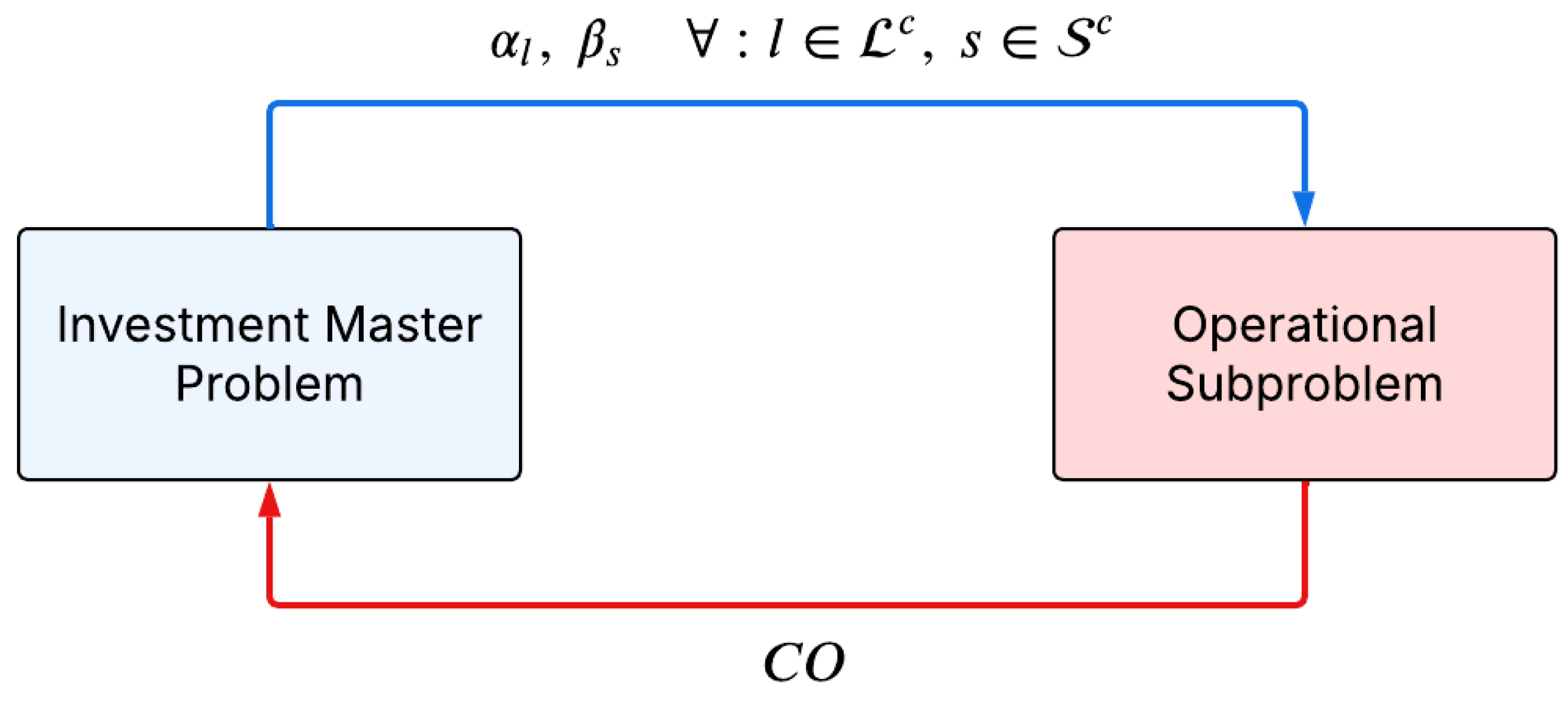
Figure 2.
Chromosome encoding.
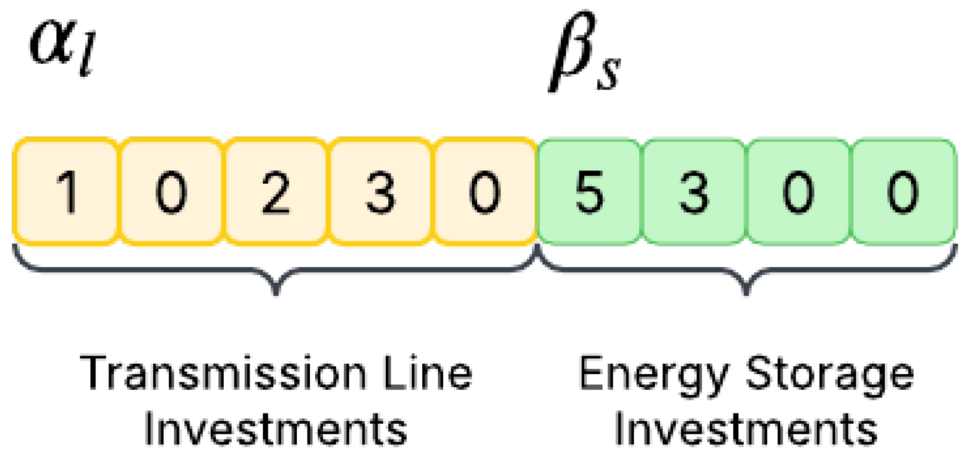
Figure 3.
Optimal operation of energy storage devices in Scenario 1 and Case IV.
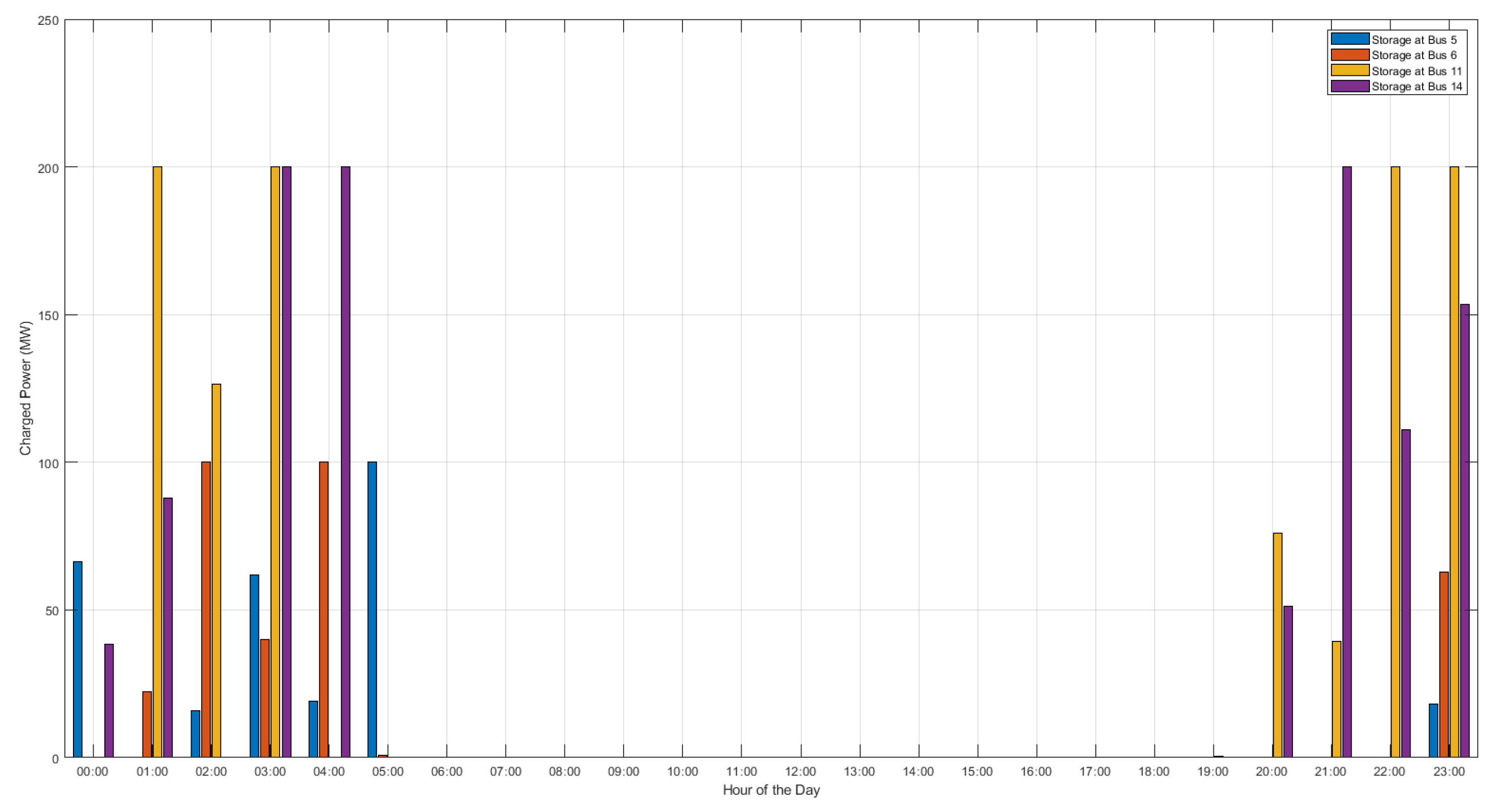
Figure 4.
Optimal operation of energy storage devices in Scenario 1 and Case IV.
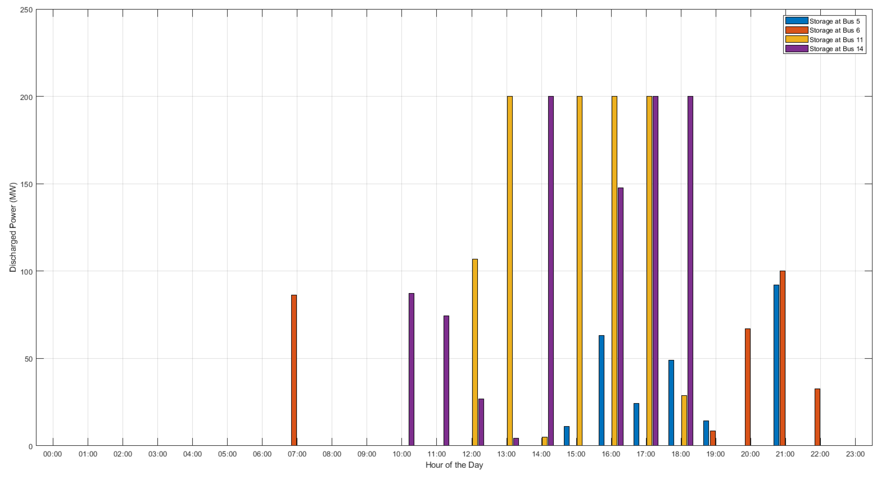

Table 1.
Taxonomy of recent publications that propose methodologies for solving co-planning of transmission and storage devices.
Table 1.
Taxonomy of recent publications that propose methodologies for solving co-planning of transmission and storage devices.
| Reference | Uncertainties | Planning horizon |
UC | Network representation |
Storage investiment |
Technology | Sistema | Model |
| [1] | No | S | No | Lossless DC | B | GESS | Garver 6-bus IEEE 24-bus Brazil 46-bus |
MILP Solver |
| [2] | No | S | No | DC | B | GESS | Garver 6-bus IEEE 24-bus |
MILP Solver |
| [3] | No | D | No | Lossless DC | B | BESS | Roy Billinton 6-bus IEEE 24-bus |
MILP Solver |
| [4] | No | S | No | Lossless DC | C | GESS | Garver 6-bus IEEE 24-bus Brazil 46-bus |
Benders Decomposition |
| [5] | Yes | D | Yes | Lossless DC | C | BESS | IEEE 24-bus IEEE 118-bus |
MILP Solver |
| [6] | No | D | No | Lossless DC | B | BESS CAES PHES |
IEEE 118-bus | Nested Benders Decomposition |
| [7] | Yes | S | No | DC | B | BESS | Garver 6-bus IEEE 24-bus |
MILP Solver |
| [8] | Yes | S | No | Lossless DC | C | BESS | WECC system 240-bus | CCG |
| [9] | Yes | S | No | Lossless DC | B | GESS | IEEE 24-bus | Benders Decomposition |
| [10] | Yes | S | No | Lossless DC | B | GESS | IEEE 24-bus | Benders Decomposition |
| [10] | Yes | S | No | Lossless DC | B | GESS | IEEE 24-bus | Benders Decomposition |
| [11] | Yes | S | No | Lossless DC | C | BESS | Garver 6-bus Chinese 196-bus |
CCG |
| [12] | Yes | D | No | Lossless DC | B | BESS PHES |
Garver 6-bus Gansu-53 bus |
Benders Decomposition |
| [13] | No | S | No | AC | C | BESS | IEEE 24-bus | Benders Decomposition |
| [14] | No | S | No | Lossless DC | B | CAES | Garver 6-bus IEEE 24-bus |
MILP Solver |
| [15] | Yes | S | No | Lossless DC | B | BESS | Garver 6-bus IEEE 24-bus IEEE 118-bus |
Benders Decomposition |
| This Work | Yes | S | Yes | Lossless DC | B | GESS | IEEE 24-bus | Decomposition GA MILP Solver |
Table 2.
Parameters of the genetic algorithm.
| Parameters | Value |
|---|---|
| Number of Chromosomes | 20 |
| Maximum number of Iterations | 50 |
| Crossover Rate | 0.7 |
| Mutation Rate | 0.3 |
| Number of Tournament Participants | 4 |
| Size of the Elite Set | 2 |
Table 3.
Best solution for each case.
| Case | Total investment cost in lines (M$) |
Total investment cost in storage (M$) |
Annual operational cost (M$) |
Transmission expansion |
Storage expansion |
|---|---|---|---|---|---|
| A | 1,494.0 | - | 42,702.86 | 1-5 (2), 2-6, 3-9, 4-9, 6-10, 7-8, 9-11 (2), 9-12, 11-14 (2), 12-13 (2), 12-23, 14-16, 15-16, 16-17, 17-22 (2), 18-21, 20-23, 1-8 (2), 6-7 (3), 14-23 |
- |
| B | 1,193.00 | 81,60 | 31,520.56 | 1-5 (2), 2-6, 3-9, 3-24, 4-9, 5-10, 6-10, 7-8 (2), 8-9, 9-11, 10-11, 11-14, 12-23, 14-16, 15-21, 15-24, 16-17, 17-18, 17-22, 20-23, 1-8 (2), 13-14, 14-23 (2) |
5 (1), 6 (1), 11 (2), 14 (2) |
Table 4.
Best solution for each case.
| Case | Stochastic Thermal Generation (MWh) |
Stochastic Charging Energy (MWh) |
Stochastic Discharging Energy (MWh) |
Stochastic Wind Curtailment (MWh) |
|---|---|---|---|---|
| A | 43,171.06 | - | - | 391.72 |
| B | 43,083.81 | 2.800.79 | 2,527.72 | 31.40 |
Table 5.
Power Generation Schedule of the Optimal Solution for Case A - First Scenario.
| Hour | Power generation of units (MW) | |||||||||||
|---|---|---|---|---|---|---|---|---|---|---|---|---|
| 1 | 197.67 | 30.40 | 0 | 0 | 0 | 0 | 54.25 | 0 | 101.25 | 600.00 | 108.50 | 140.00 |
| 2 | 133.19 | 30.40 | 0 | 0 | 0 | 0 | 54.25 | 0 | 102.57 | 600.00 | 0 | 140.00 |
| 3 | 90.44 | 30.40 | 0 | 0 | 0 | 0 | 100.40 | 0 | 0 | 600.00 | 0 | 140.00 |
| 4 | 74.42 | 30.40 | 0 | 0 | 0 | 0 | 94.68 | 0 | 0 | 600.00 | 0 | 140.00 |
| 5 | 77.64 | 30.40 | 0 | 0 | 0 | 0 | 54.25 | 0 | 100.00 | 572.26 | 0 | 140.00 |
| 6 | 112.00 | 30.40 | 0 | 0 | 0 | 0 | 54.25 | 172.21 | 0 | 600.00 | 0 | 140.00 |
| 7 | 290.92 | 59.88 | 0 | 0 | 0 | 0 | 54.25 | 479.54 | 0 | 600.00 | 0 | 169.49 |
| 8 | 304.00 | 216.76 | 0 | 0 | 0 | 0 | 54.25 | 548.09 | 0 | 600.00 | 0 | 363.13 |
| 9 | 304.00 | 278.27 | 75.00 | 0 | 0 | 0 | 54.25 | 593.20 | 0 | 600.00 | 0 | 543.89 |
| 10 | 304.00 | 286.44 | 125.64 | 0 | 0 | 0 | 58.51 | 635.42 | 0 | 600.00 | 0 | 629.94 |
| 11 | 304.00 | 291.65 | 183.89 | 0 | 0 | 0 | 83.65 | 666.23 | 0 | 600.00 | 0 | 656.30 |
| 12 | 304.00 | 293.57 | 205.36 | 0 | 0 | 0 | 92.39 | 686.24 | 0 | 600.00 | 0 | 680.72 |
| 13 | 304.00 | 297.49 | 249.21 | 0 | 0 | 0 | 112.70 | 698.56 | 0 | 600.00 | 0 | 691.21 |
| 14 | 304.00 | 301.18 | 290.40 | 0 | 0 | 0 | 132.23 | 706.28 | 0 | 600.00 | 0 | 693.36 |
| 15 | 304.00 | 300.87 | 286.99 | 0 | 0 | 0 | 130.90 | 701.81 | 0 | 600.00 | 0 | 687.63 |
| 16 | 304.00 | 303.12 | 312.10 | 0 | 0 | 0 | 143.34 | 700.74 | 0 | 600.00 | 0 | 684.49 |
| 17 | 304.00 | 265.65 | 499.92 | 0 | 0 | 0 | 201.23 | 710.52 | 0 | 600.00 | 0 | 682.46 |
| 18 | 304.00 | 248.98 | 544.69 | 0 | 0 | 0 | 211.25 | 700.82 | 0 | 600.00 | 0 | 666.64 |
| 19 | 304.00 | 250.80 | 539.80 | 0 | 0 | 0 | 214.74 | 647.02 | 0 | 600.00 | 0 | 595.51 |
| 20 | 304.00 | 304.00 | 354.63 | 0 | 0 | 0 | 173.22 | 572.58 | 0 | 600.00 | 0 | 510.10 |
| 21 | 304.00 | 296.48 | 236.69 | 0 | 0 | 0 | 89.20 | 492.86 | 0 | 600.00 | 0 | 435.96 |
| 22 | 304.00 | 222.33 | 75.00 | 0 | 0 | 0 | 0 | 416.73 | 0 | 600.00 | 0 | 371.06 |
| 23 | 253.74 | 40.32 | 75.00 | 0 | 0 | 0 | 0 | 300.58 | 0 | 600.00 | 0 | 140.00 |
| 24 | 109.81 | 0 | 75.00 | 0 | 0 | 0 | 0 | 125.79 | 0 | 600.00 | 0 | 0 |
Table 6.
Power Generation Schedule of the Optimal Solution for Case B - First Scenario.
| Hour | Power generation of units (MW) | |||||||||||
|---|---|---|---|---|---|---|---|---|---|---|---|---|
| 1 | 2 | 3 | 4 | 5 | 6 | 7 | 8 | 9 | 10 | 11 | 12 | |
| 1 | 30.40 | 30.40 | 0 | 0 | 0 | 0 | 54.25 | 0 | 373.36 | 600.00 | 108.50 | 140.00 |
| 2 | 30.40 | 30.40 | 0 | 0 | 0 | 0 | 0 | 0 | 601.29 | 600.00 | 108.50 | 0 |
| 3 | 30.40 | 30.40 | 0 | 0 | 0 | 0 | 0 | 0 | 434.06 | 600.00 | 108.50 | 0 |
| 4 | 73.42 | 30.40 | 0 | 0 | 0 | 0 | 0 | 0 | 628.96 | 600.00 | 108.50 | 0 |
| 5 | 30.40 | 30.40 | 0 | 0 | 0 | 0 | 0 | 0 | 524.33 | 600.00 | 108.50 | 0 |
| 6 | 30.40 | 30.40 | 0 | 0 | 0 | 0 | 0 | 0 | 440.52 | 600.00 | 108.50 | 0 |
| 7 | 59.07 | 30.40 | 0 | 0 | 0 | 0 | 0 | 0 | 722.64 | 600.00 | 241.96 | 0 |
| 8 | 81.49 | 30.40 | 0 | 0 | 0 | 0 | 0 | 100.00 | 788.85 | 600.00 | 399.29 | 0 |
| 9 | 302.11 | 71.97 | 0 | 0 | 0 | 0 | 0 | 150.39 | 800.00 | 600.00 | 524.16 | 0 |
| 10 | 304.00 | 129.37 | 0 | 0 | 0 | 0 | 0 | 186.60 | 800.00 | 600.00 | 619.98 | 0 |
| 11 | 230.15 | 232.75 | 0 | 0 | 0 | 0 | 0 | 215.68 | 800.00 | 600.00 | 620.00 | 0 |
| 12 | 282.37 | 258.96 | 0 | 0 | 0 | 0 | 0 | 226.42 | 800.00 | 600.00 | 620.00 | 0 |
| 13 | 304.00 | 268.98 | 0 | 0 | 0 | 0 | 0 | 226.47 | 800.00 | 600.00 | 620.00 | 0 |
| 14 | 304.00 | 268.30 | 0 | 0 | 0 | 0 | 0 | 230.92 | 800.00 | 600.00 | 620.00 | 0 |
| 15 | 304.00 | 269.52 | 0 | 0 | 0 | 0 | 0 | 213.57 | 800.00 | 600.00 | 620.00 | 0 |
| 16 | 304.00 | 271.93 | 0 | 0 | 0 | 0 | 0 | 240.66 | 800.00 | 600.00 | 620.00 | 0 |
| 17 | 304.00 | 287.82 | 0 | 0 | 0 | 0 | 0 | 241.26 | 800.00 | 600.00 | 620.00 | 0 |
| 18 | 304.00 | 276.08 | 0 | 0 | 0 | 0 | 0 | 252.16 | 800.00 | 600.00 | 620.00 | 0 |
| 19 | 304.00 | 285.72 | 0 | 0 | 0 | 0 | 0 | 264.52 | 800.00 | 600.00 | 620.00 | 0 |
| 20 | 304.00 | 273.30 | 0 | 0 | 0 | 0 | 0 | 198.99 | 800.00 | 600.00 | 620.00 | 0 |
| 21 | 304.00 | 152.00 | 0 | 0 | 0 | 0 | 0 | 132.26 | 800.00 | 600.00 | 526.89 | 0 |
| 22 | 147.71 | 0 | 0 | 0 | 0 | 0 | 0 | 100.00 | 800.00 | 558.74 | 429.90 | 0 |
| 23 | 171.29 | 0 | 0 | 0 | 0 | 0 | 0 | 0 | 747.20 | 591.09 | 178.50 | 0 |
| 24 | 139.23 | 0 | 0 | 0 | 0 | 0 | 0 | 0 | 608.18 | 597.87 | 0 | 0 |
Disclaimer/Publisher’s Note: The statements, opinions and data contained in all publications are solely those of the individual author(s) and contributor(s) and not of MDPI and/or the editor(s). MDPI and/or the editor(s) disclaim responsibility for any injury to people or property resulting from any ideas, methods, instructions or products referred to in the content. |
© 2025 by the authors. Licensee MDPI, Basel, Switzerland. This article is an open access article distributed under the terms and conditions of the Creative Commons Attribution (CC BY) license (http://creativecommons.org/licenses/by/4.0/).
Copyright: This open access article is published under a Creative Commons CC BY 4.0 license, which permit the free download, distribution, and reuse, provided that the author and preprint are cited in any reuse.


