
Submitted:
24 July 2023
Posted:
25 July 2023
You are already at the latest version
Abstract
Electrical energy demand increase does evolve rapidly due to several socioeconomic factors such as industrialization, population growth, urbanization and of course the evolution of modern technologies in this 4th industrial revolution era. Such rapid increase in energy demand introduces a huge challenge in power system. Such has paved way for network operators to seek for alternative energy resources other than the conventional fossil fuel system. Hence, the penetration of renewable energy into the electricity supply mix has evolved rapidly in the past three decades. However, the grid system has to be well planned ahead to accommodate such increase in energy demand in the long run. Transmission Network Expansion Planning (TNEP) is a well ordered and profitable expansion of power facilities that meets the expected electric energy demand with an allowable degree of reliability. This paper proposes a TNEP model that minimises the network reinforcements, operational costs and costs of renewable energy penetrations, while satisfying the increase in demand. The problem is formulated as a mixed integer linear programming (MILP) problem. The developed model has been tested in several IEEE test systems in multi-period scenarios. The paper also carried out a detailed derivation of the new non-negative variables in terms of the power flow magnitudes, the bus voltage phase angles and the lines’ phase angles for proper mixed integer variables’ decomposition techniques. Moreover, this paper tends to provide additional recommendation in terms of which particular year (within 20 years of planning period) can the network operators install new line(s), new corridor(s) and/or additional generation capacity to the respective existing power networks. Such is achieved by running incremental periods simulations from base year through the planning horizon. The results show the efficacy of the developed model in solving the TNEP problem with a reduced and acceptable computation time even for large power grid system.
Keywords:
Alternating Current Model
; Direct Current Model
; Energy Demand
; Mixed Integer Linear Programming
; Maximum Generation Capacity
; Optimal Generation Capacity
; Renewable Energy Penetration
; Transmission Network Expansion Planning.
1. Introduction
1.1. Motivation
The term, Transmission Network Expansion Planning (TNEP) refers to a periodical measure that must be carried out due to dynamic societies that attract extra energy demands [1,2]. It is the core problem in energy system expansion and economic development planning. The main target is to obtain a minimum cost for long term expansion of the transmission network capacity and as well as the generation capacity among a set of certain constraints such as the laws of energy conservation, weather, social, economic, technical and even political constraints [1,2,3,4,5].
The TNEP problem is normally a mixed integer, non-linear, non-convex optimisation problem which aims to optimal selection of the routes, types, and number of the new circuits to be added in order to face the expected future predicted load forecasting at minimum costs [6,7]. The commercial-based planning in transmission expansion takes into consideration the existing economic status, system reliability constraints, security [7,8] and the risk of planning strategies due to several uncertainties [9].
Moreover, improved reliability in high quality energy supply must correlate with the available funds. Hence, TNEP is one of the major strategic decisions in power system planning and optimisation, where the major goal is to expand the existing network by integrating new generation units, reinforcing the existing power lines, creating new transmission corridors and/or adding new power lines in order to prepare against the increasing future energy demand, thereby maintaining the system’s reliability and efficiency [6,10].
TNEP also has a crucial aspect, which is the integration of renewable energy generation units to form a large-scale grid system to satisfy the high demand in energy [5,11]. The integration of renewable energy sources to the grid is crucial due to clean energy needs to meet the emission reduction targets [12]. However, the renewable energy intermittent behaviour and its stochastic nature introduce uncertainties in TNEP, which necessitates the use of fast solution technique that can explicitly cope such uncertainties[11,13].
The major reasons for TNEP are due to large-scale grid upgrades necessary to accommodate renewable generations due to high demand in energy and as well as increase in cross-border capacity, which is good for economic growth[5,11].
Due to the fact that the location of renewable energy sources is usually in remote places, additional transmission capacities are usually needed to link them to the power grid [14].
Integration of renewable energy sources in power network expansion planning is crucial due to emission reduction targets and clean energy supply to the grid [12]. However, renewable energy sources pose further challenges in TNEP process [13].
The numerous variables, which exist in energy system expansion problems give way to several mathematical models developments designed for a suitable systematic way of obtaining the optimal solution to long term planning in power network expansion. The planning must take into account the current and future technical and economic environment within which the power sector is expected to exist. Optimal solution is the minimization of the discounted cash flow, both operating expenses and available capital over the long term period. Such is expected to reduce the effects of uncertainties beyond the given period [4].
1.2. Related Literature
The need for sustainable energy supply in the modern society, has led to numerous research approaches to improve electric energy system reliability. In this regard, the previous work of the author, Hamam [15] applied a partitioning algorithm based on Benders’ decomposition technique for the solution of a long-term power-plant mix problems. The algorithm makes possible the solution of a large problem in a limited computer memory. The special properties of the partial problems of the partitioned problem are exploited to reduce further memory requirements and computation time. The method has been implemented on the SEL 32/55 computer of the UNERG at Charleroi in Belgium.
A multi-agent Double Deep Q Network (DDQN) based on deep learning for solving the TNEP problem with high penetration of renewable energy under uncertainty is proposed in [16]. An algorithm termed as "K-means" is used to enhance the extraction quality of variable of load power and wind uncertain characteristics. The built bi-level TNEP model tend to evaluate the stability and economy of the network by solving the comprehensive cost, wind curtailment and load shedding.
Dynamic generation and transmission expansion planning considering switched capacitor bank allocation and demand response program is presented in [17]. The model is formulated in form of four-objective optimisation to supply flexible-secure and reliable energy to the grid. The model aims to minimising the planning costs, expected pollution, expected energy not-supplied, and voltage security index in separate objective functions.
A stochastic optimisation model applied to the transmission network in India to identify the optimal expansion strategy in the period from 2020 until 2060, considering conventional network reinforcements and energy storage investments is proposed in [18]. An advanced Nested Benders decomposition algorithm are used to overcome the complexity of the multistage stochastic optimisation problem with the consideration of the uncertainty around the future investment cost of energy storage.
Li, Can, et al. in [19], extended the TNEP model that was proposed in [20], by introducing three different formulations, i.e., a big-M formulation, a hull formulation, and an alternative big-M formulation. The proposed model typically involves millions or tens of millions of variables, which makes the model not directly solvable by the commercial solvers. However, such computational challenge are tackled by using a nested Benders decomposition algorithm and a tailored Benders decomposition algorithm that exploit the structure of the problem, where a case study from Electric Reliability Council of Texas (ERCOT), shows that the proposed tailored Benders decomposition outperforms the nested Benders decomposition.
Increase in uncertainty when combining a significant share of renewable energy sources in large grid planning and finding the optimal design of large grid along with its modular development plan over a long period of time are the major issues addressed in [21].
A multi-dimensional generation expansion with distributed generation resources, demand response and load management is proposed in [22]. The difficulties in handling hybrid and non-convergent mixed integer problems is alleviated using the popular nature inspired adaptive particle swarm optimisation. The classification of the proposed is in two levels, the first and the second levels. In the first level, the generation and transmission model developments are based on large-scale power plants as well as solar and wind farms. While the second level, tends to reduce the power fluctuations caused by the distributed and the non-stochastic power generation units such as micro turbines, gas turbines and combined heat and power [23].
Moreover, a novel approach to obtaining an optimal multi-period generation expansion with penetration of renewable and non-renewable energy sources is proposed in [24]. The proposed model incorporates multi-objective mathematical modeling approach, where Auto-regressive Integrated Moving Average (ARIMA) econometric method is adopted to forecast the network’s demand during the course of the planning process.
In terms of the solution algorithms, the optimisation solution algorithms compared to their heuristic and nature inspired counterparts, produce the best possible solution to various planning and scheduling problems. Planners may easily make optimised decisions and achieve higher levels of productivity and performance using optimisation solution algorithms. Generation of optimal solutions, which outperform their heuristic counterparts and enable businesses to maximize cost and operational-efficiency is eminent [25]. Morquech et al. [1] proposed an improved Differential Evolution (DE) and Continuous Population Based Incremental Learning (PBILc) hybrid solution method (IDE-PBILc), which drastically improves calculation time and robustness. They Compared the results with two different state-of-the-art meta-heuristics. Despite the fact that uncertainties are not considered in the work, the proposed approach could be of particular use when studying systems with high renewable energy penetration scenarios, due to its computational efficiency.
Furthermore, the major benefit of optimisation models is their flexibility; they may automatically adapt and adjust to accommodate the myriad decision variables and changing objectives, constraints, and complexities in any proposed problem and yield the best possible planning and scheduling solutions. However, optimisation algorithms normally take more time to execute, as they are mathematically difficult to solve [25].
Moreover, Mahdavi et al [6], evaluates lines repair and maintenance impacts on generation-transmission expansion planning (GTEP), considering the transmission and generation reliability. The objective is to form a balance between the transmission and generation expansion and operational costs and reliability, as well as lines repair and maintenance costs. For this purpose, the transmission system reliability is represented by the value of loss of load (LOL) and load shedding owing to line outages, and generation reliability is formulated by the LOL and load shedding indices because of transmission congestion and outage of generating units. The implementation results of the model on the IEEE RTS show that including line repair and maintenance as well as line loading in GTEP leads to optimal generation and transmission plans and significant savings in expansion and operational costs.
1.3. Scope and Contribution
This paper presents an optimisation approach to TNEP that minimizes the network reinforcements, operational cost and cost of renewable energy penetration, while satisfying the increase in demand. The problem is formulated as a mixed integer linear programming (MILP) problem and the developed model has been tested in several IEEE test systems in a multi-period scenarios.
The novelty of this paper is the incremental period simulations approach, which provides additional information in terms of which particular year (within the 20 years of planning period) can the network operators install new line(s), new corridor(s) and/or additional generation capacity to the respective existing power networks.
In other words, for each simulation, the program outputs the recommendations to be undertaken for reinforcing the elements of the network such as lines, new corridors, fossil fuel and renewable energy generators. The addition of such elements is suggested at appropriate times during the planning period with their corresponding investments and operation costs
Moreover, the paper showcases that the proposed model can handle large power grid systems within relatively acceptable finite computation times.
1.4. The Paper Structure
The rest of the sections of the paper are organized as follows: Section 2, introduces the TNEP problem formulation; the AC and DC TNEP problem formulations are presented in sub Section 2.1 and Section 2.2 respectively. The matrix expansion of the DC TNEP Model is presented in sub Section 2.3. Section 3 contains the results and discussions of the test cases, followed by conclusion, acknowledgements, appendices and references.
2. Transmission Network Expansion Problem Formulation
2.1. AC TNEP Problem Formulation
The formulation of AC TNEP takes into account the exact power flow equations. The description of the problem entails the incorporation of the real and reactive components of the fossil fuel and the renewable energy generations, voltage magnitude and phase information at each bus for a particular load scenario with regards to the voltage level of each generator, the line conductance, the line susceptance, the phase angle of the line, the real and reactive components of the available loads.
With such information, the active and reactive AC power flows in each branch of the network may be determined by finding the feasible solution to a set of nonlinear nodal balance equations [3], as shown in (1) and (2).
Based on the assumption of a quadratic cost curves of the generators, AC OPF model may be represented as a quadratic programming model, which the objective function, tends to minimize the total energy cost without the consideration of the unit commitment problem as shown from (3) to (23) [26].
Minimize:
subject to:
and are real and reactive power flows of the line. is the maximum flow limit of each branch. The forward and the reverse direction of flow of the real and reactive power flows are represented as , and respectively.
The available generator capacities are assumed to be constant in the steady state, hence, the unit commitment problem is not considered in the model and the phase angle difference is kept small for security purposes.
2.2. DC TNEP Problem Formulation
The formulation of the DC TNEP takes into account the linearised version of AC TNEP with some key assumptions as follows:
- The bus voltage magnitudes must be set to 1.0 p.u.(assuming uniform bus voltage level for all buses.)
- The phase angle difference of the bus voltage is so small that
- The algebraic sum of branch flow has to be zero () hence, is negligible.
- The reactive power flow has to be zero () and
- The reactive generation has to be zero ()
Considering the above assumptions, the active power flow per branch in DC power network (6) and (7) may be simplified as shown in (24 and 25).
Similarly the DC power flow nodal balance equation may be represented as follows:
Hence, the complete linearised DC TNEP problem is formulated as shown below.
Subject to:
The DC TNEP model represents only the linear term of the original quadratic model of the AC TNEP and that brings convexity, which allows for faster computation time [27]. However, the effects of the system’s reactive power and losses remain non-salient in that case.
2.3. Explicit Matrix Expansion of the DC TNEP Model
The expansion of the developed model in terms of matrices is essential for proper representation of the model in any suitable optimisation software. The DC TNEP model in generic matrix form represented from (38) to (53) and the summary is shown in Table 1.
Subject to:
2.4. Relaxation of the Negative Variables
In order to carry out the multi-period simulation of the developed model, it is necessary to derive new non-negative variables that can avoid negative variables in terms of the power flow of the lines, line phase angles and the bus phase angles.
The derivation for new non-negative variables may be established by rearranging the respective limits of the mentioned negative variables of the respective constraints of the already developed TNEP model (refer to 38-53 ), as follows;
Let the new variables for existing and new power flows, line angle and bus angle respectively be , , and .
Hence,
The reformulations of the problem with respect to the new variables are as follows:
Subject to:
3. Results and Discussions of the Test Cases
This section presents the simulation results of the proposed model. The model are being tested with four test cases of IEEE test systems.
The planning horizon for the period of increase in energy demand is assumed to be from 2024 to 2045.
The simulations were conducted in two different states of the power networks. The first simulation was conducted on the initial state of networks’ base year to obtain the present state of the network, and the second simulation was conducted with a compound increment demand factor, per-annum for the 20 years’ planning horizon, which varies according to the nature of the demands of each network test system.
Hence, the future value, of the load at the end of the planning horizon is related to base value, as follows:
Where the reciprocal of the expression is the discount factor of the overall demand cost.
The adopted annual load duration curve (for the study) has an assumed 20 periods per annum with randomised different demand states at different times of the year as shown in Figure 1.
The obtained results in terms of network reinforcements, new corridors and generations sources represent the recommendation for the long term investment and operation of the power system. However, such may be reviewed annually, should there be a new development that may incur additional energy demand that was not included in the previous planning.
Moreover, the approach taken in this paper also provides an additional recommendation in terms of which particular year (within the 20 years of planning period) can the network operators install new line(s), new corridor(s) and/or additional generation capacity to the respective existing power networks. Such may be achieved by running incremental periods simulations from base year through the planning horizon and that can aid the power network operators in predicting viable expansion for the optimal operation of the network.
The upper bounds of both fossil fuel and renewable energy generation capacities are set according to the maximum generation capacity of each generator and the lower bounds are simply set to zero in all the test cases.
MATLAB 2022b installed in an Intel(R) Core(TM) i5-2400 CPU @ 3.10GHz 3.10 GHz 8.00 GB RAM Computer with 64-bit operating system was used in conducting the simulations. The MATLAB inbuilt solver, uses cuts generation and classical linear programming technique to solve mixed integer linear problem.
The results were recorded and analysed as shown in the next subsections. The CPU computation times in terms of the different test cases of the IEEE test systems were recorded and compared.
3.1. The IEEE 6-Bus System
The IEEE 6-bus test case system has a total base year energy demand of 241 and a total expected rise in demand over the horizon is based on an annual compounded increase factor of 7%.
The base year demand and the planing horizon demand at each bus are plotted and compared as shown in Figure 2.
The optimal solution in Table 2, shows that the system needs one new corridor (5-4) and one new new line (2-5) along with the rest of the 9 existing lines to be able to satisfy the expected the increase in demand over the planning horizon.
The respective optimal generation capacities at each generator bus are shown in Table 3.
Moreover, incremental periods simulations of the planning horizon further predicted the early useful years of the IEEE 6 bus system’s new line and/or new corridors investments, as shown in Table 10.
Consequently, the incremental periods simulations also reveal the incremental steps of the generation capacities as shown in Table 11, which shows the expected different states of the generators at different periods. Moreover, it may be noticed from Table 11 that renewable energy penetration tends to grow as the time moves upwards due to the quest for global alternative renewable energy sources and urge to move away from burning fossil fuel due to its negative impacts on global warming.
3.2. The IEEE 9-Bus System Test Case Results
The TNEP model was also tested in IEEE 9-bus system. The system comprises of 9 existing transmission lines, 3 fossil fuel generators and 3 potential renewable energy sources with a total base year demand of .
The base year demand and the planing horizon demand for each bus of the network are shown in Figure 3.
With an increment rate of 8% in energy demand per annum, the optimal results in Table 4 suggest that 3 new lines and 1 new corridor should be constructed to satisfy the total energy demand over the planning period. The total optimal generation capacities at each generator bus over the horizon are shown in Table 5.
3.3. The IEEE 24-Bus System
The TNEP model was also tested in IEEE 24-bus system. The system comprises of 38 existing transmission lines, 5 fossil fuel generators and 4 potential renewable energy sources with a total base year demand of .
The base year demand and the planing horizon demand for each bus of the 24-bus network are shown in Figure 4.
With an increment rate of 8% in energy demand per annum, the optimal results in Table 6 suggest that 4 new lines and 1 new corridor should be constructed to satisfy the total energy demand over the planning period. The total optimal generation capacities at each generator bus over the horizon are shown in Table 7.
Consequently, the incremental periods simulation results further reveal the exact years in which such new lines, new corridors and the optimal generation capacities should be in optimal usable states as shown in Table 14 and Table 15 respectively. It may also be noticed (from Table 15) that renewable energy penetration occurred on the 10th year through buses 16 and 22.
3.4. The IEEE 39-Bus System
The IEEE 39-bus system test case has a total base year energy demand of 7556.73 located across 29 different load buses. The system also comprises of 46 existing transmission lines, 9 fossil fuel generators and 9 potential renewable energy sources.
The base year demand and the planning horizon demand for each bus of the 39-bus network are shown in Figure 5.
With the demand increment rate of 6.5% per annum, the optimal results in Table 16 suggest that 17 new lines and 3 new corridors should be constructed to satisfy the total energy demand over the planning period. The total optimal generation capacities at each generator bus over the horizon are shown in Table 8.
3.5. The IEEE 200-Bus System
For the purpose of reassuring robustness of the model in handling large network system, IEEE 200-bus system was adopted. The system comprises of 246 existing transmission lines, 24 fossil fuel generators and 24 potential renewable energy sources with a total base year demand of .
The base year demand and the planing horizon demand for each bus of the 200-bus network are shown in Figure 6.
Due to the demand pattern across the 200 buses, the compounded annual demand increment rate is chosen to be 4%.
The optimal results in Table 19 recommend 30 new lines and 10 new corridors to be constructed to satisfy the total energy demand over the planning period. The total optimal generation capacities in each generator bus over the horizon are shown in Table 9.
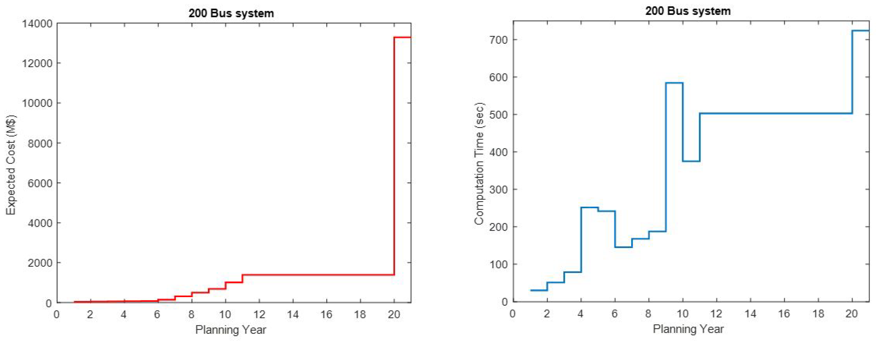
The computation times for the different tested network sizes is shown in Figure 7. And the optimal total costs of the network test systems obtained during the course of the simulation are shown in Figure 8; while, Figure 9 shows the computation time and total cost curves for the 200 bus system.
It can be noticed in Figure 7 and Figure 9 that the computation times fall within an acceptable finite time ranges for the respective test systems.
Moreover, it has been observed that higher number of candidate integer variables increases the computation times and can lead to premature termination, without reaching the optimal solution.

Table 10.
The predicted early investment year of the IEEE 6 bus system’s transmission line expansion
Table 10.
The predicted early investment year of the IEEE 6 bus system’s transmission line expansion
| 18th year | 20th year | ||
|---|---|---|---|
| fb-tb | OPF () | New Lines | New Corridors |
| 2-5 | 14.81 | 1 | - |
| 5-4 | 3.29 | - | 1 |
Table 11.
The predicted years of expected increase in generation capacities (in ) in the 6 Bus System .
Table 11.
The predicted years of expected increase in generation capacities (in ) in the 6 Bus System .
| Base Year | 3rd Year | 5th Year | 15th Year | 20th Year | ||||||
|---|---|---|---|---|---|---|---|---|---|---|
| Bus | ||||||||||
| 1 | - | - | - | - | - | - | 24.14 | - | 155.84 | - |
| 2 | - | 150 | - | - | - | - | - | 43.2 | - | 101.66 |
| 3 | - | - | - | 128.82 | - | 150 | - | 132.46 | - | 150 |
| 4 | - | - | - | - | 1.68 | - | 150 | - | 150 | - |
| 5 | 87.1 | - | 150 | - | 150 | - | 150 | - | 150 | - |
| 6 | - | - | - | 2.58 | - | 51.12 | - | 180 | - | 180 |
Table 12.
The predicted early investment year of the IEEE 9 bus system’s transmission line expansion
Table 12.
The predicted early investment year of the IEEE 9 bus system’s transmission line expansion
| 13th year | 16th year | 20th year | |||||
|---|---|---|---|---|---|---|---|
| fb-tb | OPF () | Lines | Corridors | Lines | Corridors | Lines | Corridors |
| 4-9 | 194.49 | 1 | - | - | - | - | - |
| 4-9 | 245.76 | - | - | - | - | 1 | - |
| 6-7 | 110.04 | - | - | 1 | - | - | - |
| 6-1 | 110.28 | - | - | - | - | - | 1 |
Table 13.
The predicted years of expected increase in generation capacities (in ) in the 9 Bus System.
Table 13.
The predicted years of expected increase in generation capacities (in ) in the 9 Bus System.
| Base Year | 3rd Year | 5th Year | 10th Year | 13th Year | ||||||
|---|---|---|---|---|---|---|---|---|---|---|
| Bus | ||||||||||
| 4 | - | - | - | - | - | - | - | - | 310.68 | - |
| 5 | 106 | - | 251.38 | - | 300 | - | 300 | - | 300 | - |
| 6 | - | - | - | - | - | - | - | 130.78 | - | 106.08 |
| 7 | 270 | - | 270 | - | 270 | - | 270 | - | 270 | - |
| 8 | - | - | - | - | - | 66.05 | - | 300 | - | 300 |
| 9 | - | 270 | - | 270 | - | 270 | - | 270 | - | 270 |
Table 14.
The predicted early investment year of the IEEE 24 bus system’s transmission line expansion
Table 14.
The predicted early investment year of the IEEE 24 bus system’s transmission line expansion
| 5th year | 14th year | 16th year | 20th year | ||||||
|---|---|---|---|---|---|---|---|---|---|
| fb-tb | OPF () | Lines | Cors | Lines | Cors | Lines | Cors | Lines | Cors |
| 15-1 | 175 | - | 1 | - | - | - | - | - | - |
| 7-8 | 175 | - | - | 2 | - | - | - | - | - |
| 13-12 | 500 | - | - | - | - | 1 | - | - | - |
| 16-19 | 406.41 | - | - | - | - | 1 | - | 1 | - |
Table 15.
The predicted years of expected increase in generation capacities (in ) in the 24 Bus System .
Table 15.
The predicted years of expected increase in generation capacities (in ) in the 24 Bus System .
| Base Year | 5th Year | 10th Year | 14th Year | 20th Year | ||||||
|---|---|---|---|---|---|---|---|---|---|---|
| Bus | ||||||||||
| 1 | - | - | 20.04 | - | - | - | - | - | 24.39 | - |
| 2 | - | - | - | - | 95.716 | - | 479.67 | - | 596.42 | - |
| 7 | - | - | 175 | - | 175 | - | 350 | - | 525 | - |
| 13 | 336.48 | - | 533.13 | - | 1131.2 | - | 1031.2 | - | 1602.3 | |
| 15 | 870.52 | - | 1045.30 | - | 1112 | - | 1112 | - | 263.06 | - |
| 16 | - | - | - | - | - | 68.17 | - | 516.38 | - | 980 |
| 21 | - | - | - | - | - | - | - | - | - | 704.79 |
| 22 | - | - | - | - | - | 23.78 | - | 55.965 | - | 929.83 |
Table 16.
The optimal results of line expansions of the IEEE 39 bus system’s expansion over the planning period
Table 16.
The optimal results of line expansions of the IEEE 39 bus system’s expansion over the planning period
| fb-tb | OPF () | New Lines | New Corridors | fb-tb | OPF () | New Lines |
|---|---|---|---|---|---|---|
| 3-18 | 500 | 1 | - | 33-19 | 900 | 1 |
| 25-4 | 500 | - | 1 | 35-22 | 712.94 | 1 |
| 6-7 | 843.53 | 1 | - | 36-23 | 687 | 2 |
| 7-16 | 480 | - | 1 | 23-22 | 545.31 | 2 |
| 11-6 | 480 | 1 | - | 20-34 | 900 | 1 |
| 39-9 | 738.28 | - | 1 | 27-17 | 566.18 | 2 |
| 17-16 | 600 | 2 | - | 16-21 | 597.93 | 2 |
| 19-16 | 513.87 | 1 | - |
Table 17.
The predicted in-use year of the IEEE 39 bus system’s transmission line extensions
| 8th year | 12th year | 16th year | 20th year | ||||
|---|---|---|---|---|---|---|---|
| fb-tb | OPF () | Lines | Lines | Cors | Lines | Lines | Cors |
| 16-21 | 390.29 | 1 | - | - | - | - | - |
| 35-22 | 762 | - | 1 | - | - | - | - |
| 7-16 | 480 | - | - | 1 | - | - | - |
| 3-18 | 500 | - | - | - | 1 | - | - |
| 34-20 | 849.74 | - | - | - | 1 | - | - |
| 17-16 | 599.08 | - | - | - | 1 | - | - |
| 27-17 | 448.30 | - | - | - | 1 | - | - |
| 23-22 | 600 | - | - | - | 1 | - | - |
| 36-23 | 809.41 | - | - | - | 1 | - | - |
| 6-7 | 843.53 | - | - | - | - | 1 | - |
| 11-6 | 480 | - | - | - | - | 1 | - |
| 17-16 | 600 | - | - | - | - | 1 | - |
| 19-16 | 513.87 | - | - | - | - | 1 | - |
| 25-4 | 500 | - | - | - | - | - | 1 |
| 39-9 | 738.28 | - | - | - | - | - | 1 |
| 16-21 | 597.93 | - | - | - | - | 1 | - |
| 27-17 | 566.18 | - | - | - | - | 1 | - |
| 33-19 | 900 | - | - | - | - | 1 | - |
| 23-22 | 545.31 | - | - | - | - | 1 | - |
| 36-23 | 687 | - | - | - | - | 1 | - |
Table 18.
The predicted years of expected change in generation capacities (in ) in the 39 Bus System.
Table 18.
The predicted years of expected change in generation capacities (in ) in the 39 Bus System.
| Base Year | 8th Year | 12th Year | 16th Year | 20th Year | ||||||
|---|---|---|---|---|---|---|---|---|---|---|
| Bus | ||||||||||
| 3 | - | 1075.3 | - | 2032.9 | - | 1221.4 | - | 1603.1 | - | 1793.5 |
| 4 | - | - | - | 726.67 | - | 1956 | - | 1956 | - | 1956 |
| 10 | - | - | - | - | - | 1027.6 | - | 1109.8 | - | 70.57 |
| 11 | - | 550.72 | - | - | - | - | - | - | 1577.9 | |
| 24 | - | 893.21 | - | 1328.7 | - | 1460.7 | - | 1704.3 | - | 1740 |
| 26 | - | - | - | - | - | - | - | - | - | 1692 |
| 27 | - | - | - | 355.25 | - | 654.06 | - | 1066.3 | - | 2121.5 |
| 28 | - | 434.33 | - | 718.82 | - | 924.74 | - | 1005.6 | - | - |
| 30 | - | - | 290.86 | - | 271 | - | 1930.4 | - | 2557.9 | - |
| 31 | - | 383.79 | - | 1815.2 | - | 916.05 | - | 1270.4 | - | 1832.4 |
| 32 | - | - | - | - | - | - | - | - | - | - |
| 33 | 430 | - | 900 | - | 900 | - | 900 | - | 1800 | - |
| 34 | 900 | - | 900 | - | 900 | - | 1699.5 | - | 1524 | - |
| 35 | 577.37 | - | 900 | - | 1524 | - | 1524 | - | 2061 | - |
| 36 | 862.89 | - | 791.65 | - | 900 | - | 1618.8 | - | 1425.9 | - |
| 37 | 249.1 | - | 546.28 | - | 734.53 | - | 900 | - | 900 | - |
| 38 | 1200 | - | 1200 | - | 1200 | - | 1200 | - | 1200 | - |
| 39 | - | - | - | - | 1499 | - | 1209.7 | - | 2098.5 | - |
Table 19.
The optimal results of line expansions of the IEEE 200 bus system’s expansion over the planning period
Table 19.
The optimal results of line expansions of the IEEE 200 bus system’s expansion over the planning period
| fb-tb | OPF () | New Lines | New Corridors | fb-tb | OPF () | New Lines |
|---|---|---|---|---|---|---|
| 11-15 | 16.67 | 1 | - | 90-89 | 8.6 | 1 |
| 11-113 | 100 | - | 1 | 38-36 | 63.26 | 1 |
| 116-15 | 14.78 | - | 1 | 29-30 | 64.74 | 1 |
| 22-123 | 22.91 | - | 1 | 158-22 | 16.67 | 1 |
| 154-34 | 77.74 | - | 1 | 76-75 | 24.3 | 1 |
| 134-137 | 24.80 | - | 1 | 107-129 | 10.61 | 1 |
| 177-31 | 83.16 | 1 | - | 112-113 | 23.80 | 1 |
| 31-192 | 74.23 | 1 | - | 114-112 | 11.05 | 1 |
| 127-158 | 23.84 | - | 1 | 67-66 | 30 | 1 |
| 140-129 | 47.46 | - | 1 | 113-192 | 22.09 | 1 |
| 136-38 | 95.92 | - | 1 | 116-117 | 90.75 | 1 |
| 136-83 | 29.94 | - | 1 | 123-124 | 271.93 | 1 |
| 77-75 | 7.4 | 1 | - | 126-123 | 148.72 | 1 |
| 79-75 | 39.60 | 1 | - | 127-123 | 170 | 1 |
| 149-114 | 2.17 | - | 1 | 93-191 | 18.69 | 1 |
| 133-128 | 58.44 | 1 | - | 134-140 | 50.36 | 1 |
| 147-146 | 130.60 | 1 | - | 146-177 | 97.55 | 1 |
| 151-149 | 10.34 | 1 | - | 164-163 | 58.1 | 1 |
| 167-163 | 39.60 | 1 | - | 168-163 | 39.60 | 1 |
| 183-181 | 39.60 | 1 | - | 196-195 | 87.70 | 1 |
Figure 7.
The several test systems’ computation times along the planning years
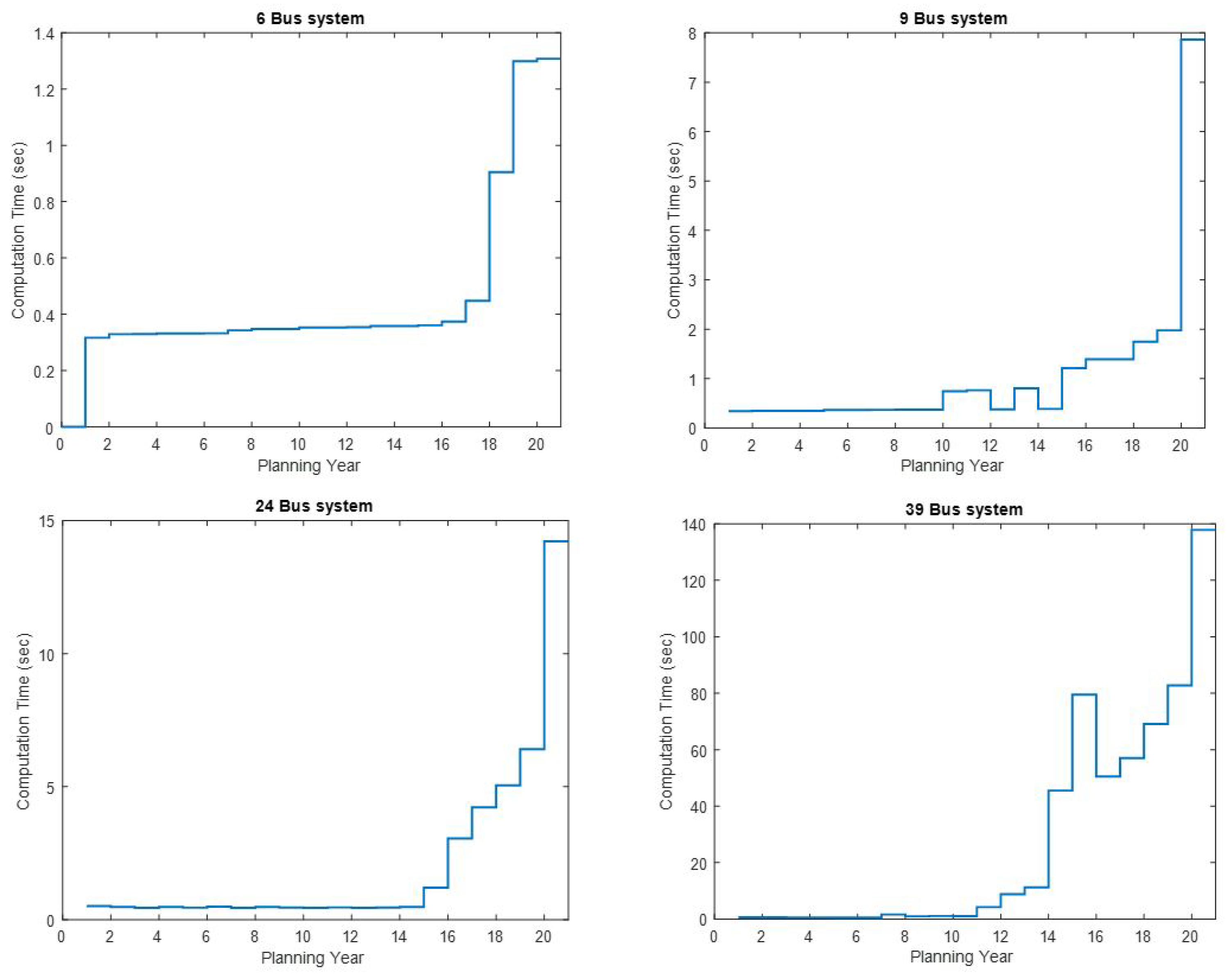
Figure 8.
The optimal total costs of the several test systems along the planning years
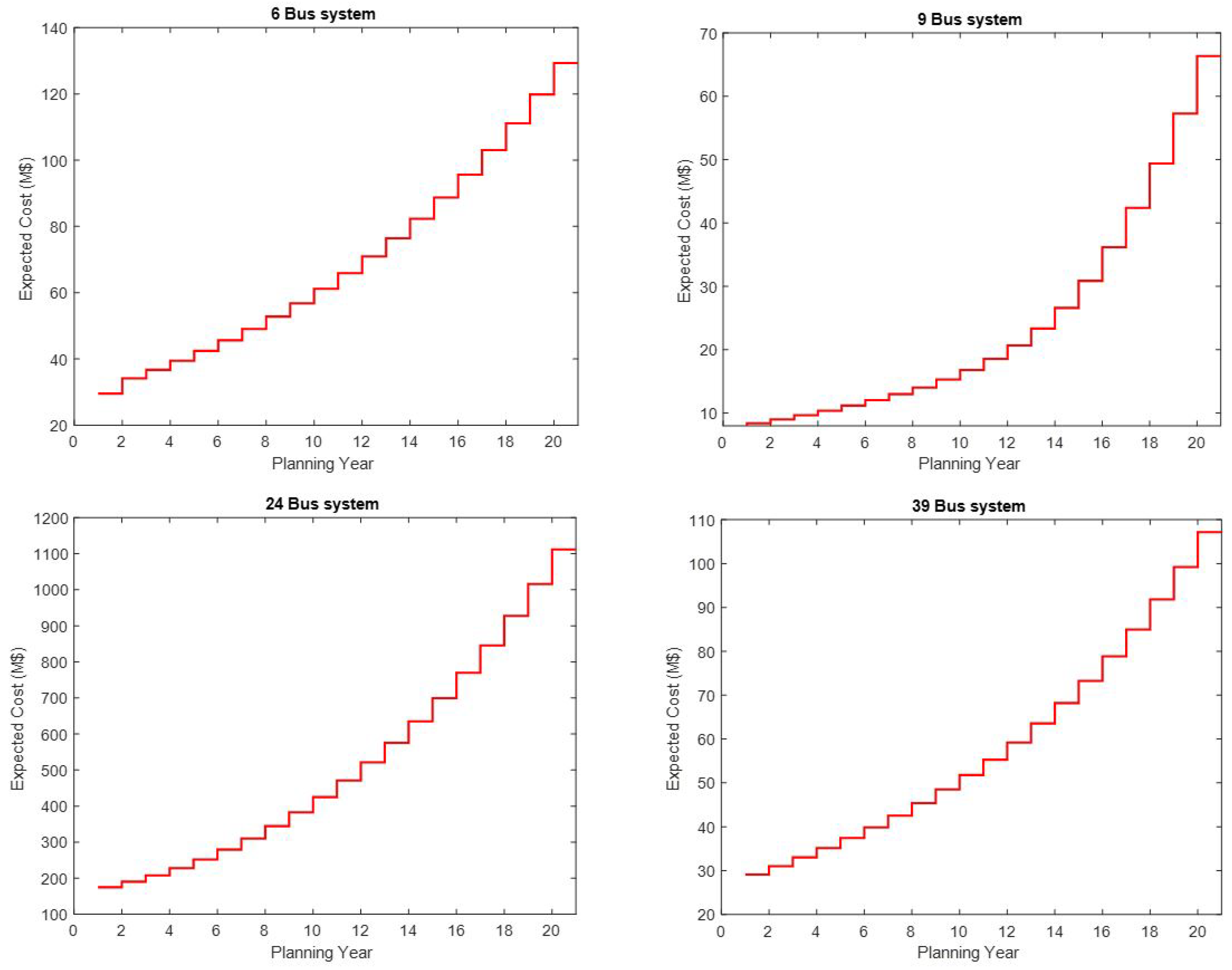
Figure 9.
The optimal total costs and the computation times in a 200 bus test system along the planning years
Figure 9.
The optimal total costs and the computation times in a 200 bus test system along the planning years
4. Conclusion
Power transmission network modelling plays a crucial role in the expansion planning procedure. It is of high important to understand the fundamental behaviour of the system, which will allow the facilitation of the formulation of an appropriate mathematical optimisation model and also aides for a better decision in the planning process. The long term planning is normally carried out on the first year of the planning horizon and the obtained results in terms of network reinforcements, new corridors and generations sources represent the recommendation for the long term investment and operation of the power system. However, such can be reviewed annually, should there be a new development that can incur additional energy demand that was not included in the previous planning. The TNEP has been tackled as a DC-TNEP problem that minimizes the investment cost of adding new circuits, operational cost and the cost of renewable energy penetration; while satisfying the increase in demand and other constraints. It is formulated as a mixed integer linear programming (MILP) model. It was tested on IEEE 6, 9, 24, 39 and 200 bus test systems within acceptable finite computation times. The discussion of the obtained results is relevant and has highlighted the value of the proposed approach. The adopted annual load duration curve has an assumed 20 periods per annum with randomized different demand states at different times of the year, which resulted to a multi-periods of 20 years TNEP horizon. The idea is to obtain the information in terms of how the generator capacities and the demand evolve annually. The major findings in this work show that the increments in demand in different test systems in use do not follow similar pattern. This is because, each of the test systems has different network characteristics in terms of the network parameters, generation and demand patterns. In order words, they do not maintain unified pattern of changes. For instance, Table 11 and Table 13, show that penetrations of renewable energy generation first occur at the base year of the planning horizon in 6 and 9-bus test systems. However, Table 15, shows that such penetrations can only start at the 10th year of the planning horizon in 24 bus test system. Hence, due to the fact that different network sizes are been used for the test cases, stages of their changes in generation capacities and demands are not uniform. Moreover, additional findings show which particular year (within the 20 years of planning period) can the network operators install new line(s), new corridor(s) and/or additional generation capacity to the respective existing power networks. Such was achieved by running incremental periods simulations from base year through the planning horizon.
Author Contributions
Formal analysis, G.U.N., Y.H. and C.G.R.; original draft preparation, G.U.N., Y.H. and C.G.R.; editing and writing—review, Y.H. and C.G.R. All authors have read and agreed to the published version of the manuscript.
Funding
This research was funded by NATIONAL RESEARCH FOUNDATION South Africa 98398.
Acknowledgments
This research work was supported by the French South African Institute of Technology (F’SATI), Tshwane University of Technology, Pretoria, South Africa
Conflicts of Interest
The authors declare no conflict of interest.
Abbreviations
- Nomenclature
The following abbreviations are used in this manuscript:
| Set | |
| d | Load buses |
| g | Fossil fuel generator buses |
| k | Transmission lines |
| ℜ | Renewable energy generator buses |
| Planning period in years | |
| Parameters | |
| Susceptance of existing transmission line k | |
| Susceptance of prospective transmission line k | |
| Susceptance of a transmission line k | |
| Operating cost coefficients of fossil fuel generators | |
| Operating cost coefficients of renewable energy sources | |
| Investment cost coefficient of new lines | |
| Conductance of transmission line k | |
| The disjunctive big-M | |
| Energy demand at load bus d | |
| Base year energy demand at bus d | |
| Planning horizon energy demand at bus d | |
| Maximum fossil fuel generation at generator bus g | |
| Maximum Renewable generation capacity of generator ℜ | |
| Maximum power flow in existing transmission line k | |
| Maximum power flow in prospective transmission line k | |
| Maximum bus voltage | |
| Minimum bus voltage | |
| Increment in energy demand factor | |
| Variables | |
| Optimal power flow in existing transmission line k | |
| Optimal power flow in prospective transmission linek | |
| Optimal fossil fuel generation capacity of generator g | |
| Optimal Renewable generation capacity of generator ℜ | |
| Prospective transmission line k | |
| Existing line k phase angle | |
| Prospective line k phase angle | |
| Phase angle of transmission line k | |
| Bus phase angle | |
| Voltage profile at bus i | |
| Voltage profile at bus j | |
| Forward direction active power flow in transmission line k | |
| Reverse direction active power flow in transmission line k | |
| Forward direction reactive power flow in transmission line k | |
| Reverse direction reactive power flow in transmission line k | |
| Apparent power flow in transmission line k | |
| Other abbreviations | |
| b | The right hand side of the constraints |
| Node-Branch incidence matrix of the existing lines | |
| Node-Branch incidence matrix of the prospective lines | |
| Branch-node incidence matrix of the existing lines | |
| Branch-node incidence matrix of the prospective lines | |
| Identity matrix of set of fossil fuel generators | |
| Identity matrix of set of renewable energy generators | |
| Identity matrix of set of existing lines in k right of way | |
| Identity matrix of set of prospective lines in k right of way | |
| Acronyms | |
| ARIMA | Auto-regressive Integrated Moving Average |
| DDQN | Double Deep Q Network |
| fb-tb | From bus to bus |
| LP | Linear programming |
| MILP | Mixed-integer linear programming |
| MINLP | Mixed-integer non-linear programming |
| MGC | Maximum Generation Capacity |
| MPF | Maximum Power Flow |
| MW | Megawatts |
| OC | Operating Cost |
| OGC | Optimal Generation Capacity |
| OPF | Optimal Power Flow |
| sec | Seconds |
| TNEP | Transmission Network Expansion Planning |
Appendix A. Matrix Expansion of the Model
In that effect, a 4-bus test system, which the line diagram is shown in Figure A1, is used for the expansion of the DC OPF model to be expressed in matrix form in terms of the general linear equality constraints notation: . The summary of the matrix expression of the model is shown in Table A1.
Figure A1.
The line diagram of a 4-Bus test system with renewable energy penetrations
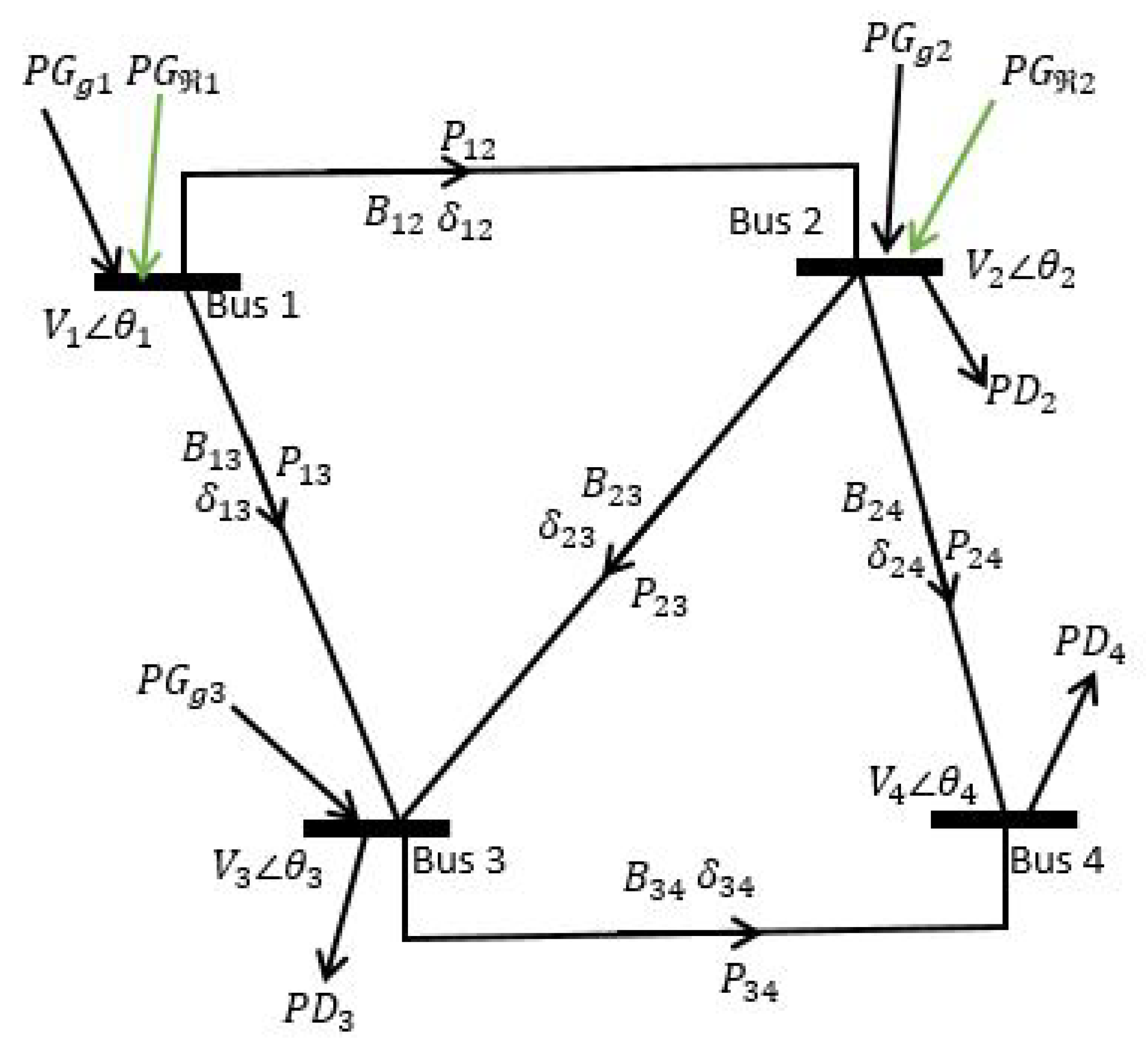
The nodal power balance constraint in ??, can be expanded in terms of the sample 4-bus system as follows:
The expression of the nodal power balance equation in matrix form is as follows:
The expansion of the active power flow in relation to the phase angle of the line is as follows:
The equivalent matrix:
The detailed relationship between the phase angles of the buses and the branch phase angles of the 4-bus test system is expressed as follows:
The expression of the bus phase angles versus branch angles in matrix form is as follows:
The constraint for adding new lines as shown in ?? and ??, can be expanded in terms of the sample 4-bus system as follows.
The lower bound:
The upper bound:
The matrix representation of the lower and upper bounds of the new lines constraint.
The lower bound matrix:
The upper bound matrix:
Table A1.
The summary of the TNEP Matrix Model.
| b | ||||||
|---|---|---|---|---|---|---|
| 0 | 0 | 0 | ||||
| 0 | 0 | 0 | 0 | 0 | ||
| 0 | C | 0 | 0 | 0 | 0 | |
| 0 | 0 | 0 | ||||
| 0 | 0 | 0 | ||||
| 0 | 0 | 0 | 0 | 0 | ||
| 0 | 0 | 0 | 0 | 0 |
References
- Morquecho, E.G.; Torres, S.P.; Astudillo-Salinas, F.; Castro, C.A.; Ergun, H.; Van Hertem, D. Security constrained AC dynamic transmission expansion planning considering reactive power requirements. Electric Power Systems Research 2023, 221, 109419. [Google Scholar] [CrossRef]
- Ude, N.G.; Yskandar, H.; Graham, R.C. A comprehensive state-of-the-art survey on the transmission network expansion planning optimization algorithms. IEEE Access 2019, 7, 123158–123181. [Google Scholar]
- Vellingiri, M.; Rawa, M.; Alghamdi, S.; Alhussainy, A.A.; Ali, Z.M.; Turky, R.A.; Refaat, M.M.; Aleem, S.H.A. Maximum hosting capacity estimation for renewables in power grids considering energy storage and transmission lines expansion using hybrid sine cosine artificial rabbits algorithm. Ain Shams Engineering Journal 2023, 14, 102092. [Google Scholar] [CrossRef]
- Covarrubias, A. Expansion planning for electric power systems. IAEA Bulletin 1979, 21, 55–64. [Google Scholar]
- Hemmati, R.; Hooshmand, R.A.; Khodabakhshian, A. State-of-the-art of transmission expansion planning: Comprehensive review. Renewable and Sustainable Energy Reviews 2013, 23, 312–319. [Google Scholar] [CrossRef]
- Mahdavi, M.; Javadi, M.S.; Catalão, J.P. Integrated generation-transmission expansion planning considering power system reliability and optimal maintenance activities. International Journal of Electrical Power & Energy Systems 2023, 145, 108688. [Google Scholar]
- Shaheen, A.M.; El-Sehiemy, R.A. Application of multi-verse optimizer for transmission network expansion planning in power systems. 2019 International Conference on Innovative Trends in Computer Engineering (ITCE), IEEE, 2019; 371–376. [Google Scholar]
- Gan, W.; Ai, X.; Fang, J.; Yan, M.; Yao, W.; Zuo, W.; Wen, J. Security constrained co-planning of transmission expansion and energy storage. Applied Energy 2019, 239, 383–394. [Google Scholar] [CrossRef]
- Khodaei, A.; Shahidehpour, M.; Kamalinia, S. Transmission switching in expansion planning. IEEE Transactions on Power Systems 2010, 25, 1722–1733. [Google Scholar] [CrossRef]
- Zhang, X.; Conejo, A.J. Candidate line selection for transmission expansion planning considering long-and short-term uncertainty. International Journal of Electrical Power & Energy Systems 2018, 100, 320–330. [Google Scholar]
- Ramos, A.; Lumbreras, S. How to solve the transmission expansion planning problem faster: acceleration techniques applied to Benders’ decomposition. IET Generation, Transmission & Distribution 2016, 10, 2351–2359. [Google Scholar]
- Lumbreras, S.; Ramos, A. Transmission expansion planning using an efficient version of Benders’ decomposition. A case study. In PowerTech (POWERTECH), 2013 IEEE Grenoble; IEEE, 2013; pp. 1–7. [Google Scholar]
- Zambrano, C.; Arango-Aramburo, S.; Olaya, Y. Dynamics of power-transmission capacity expansion under regulated remuneration. International Journal of Electrical Power & Energy Systems 2019, 104, 924–932. [Google Scholar]
- Zhang, H.; Heydt, G.T.; Vittal, V.; Quintero, J. An improved network model for transmission expansion planning considering reactive power and network losses. IEEE Transactions on Power Systems 2013, 28, 3471–3479. [Google Scholar] [CrossRef]
- Hamam, Y.; Renders, M.; Trecat, J. Partitioning algorithm for the solution of long-term power-plant mix problems. In Proceedings of the Institution of Electrical Engineers; IET, 1979; Volume 126, pp. 837–839. [Google Scholar]
- Wang, Y.; Zhou, X.; Shi, Y.; Zheng, Z.; Zeng, Q.; Chen, L.; Xiang, B.; Huang, R. Transmission Network Expansion Planning Considering Wind Power and Load Uncertainties Based on Multi-Agent DDQN. Energies 2021, 14, 6073. [Google Scholar] [CrossRef]
- Davoodi, A.; Abbasi, A.R.; Nejatian, S. Multi-objective dynamic generation and transmission expansion planning considering capacitor bank allocation and demand response program constrained to flexible-securable clean energy. Sustainable Energy Technologies and Assessments 2021, 47, 101469. [Google Scholar] [CrossRef]
- Giannelos, S.; Jain, A.; Borozan, S.; Falugi, P.; Moreira, A.; Bhakar, R.; Mathur, J.; Strbac, G. Long-Term Expansion Planning of the Transmission Network in India under Multi-Dimensional Uncertainty. Energies 2021, 14, 7813. [Google Scholar] [CrossRef]
- Li, C.; Conejo, A.J.; Liu, P.; Omell, B.P.; Siirola, J.D.; Grossmann, I.E. Mixed-integer linear programming models and algorithms for generation and transmission expansion planning of power systems. European Journal of Operational Research 2022, 297, 1071–1082. [Google Scholar] [CrossRef]
- Lara, C.L.; Mallapragada, D.S.; Papageorgiou, D.J.; Venkatesh, A.; Grossmann, I.E. Deterministic electric power infrastructure planning: Mixed-integer programming model and nested decomposition algorithm. European Journal of Operational Research 2018, 271, 1037–1054. [Google Scholar] [CrossRef]
- Pache, C.; Maeght, J.; Seguinot, B.; Zani, A.; Lumbreras, S.; Ramos, A.; Agapoff, S.; Warland, L.; Rouco, L.; Panciatici, P. New Methodology for Long-Term Transmission Grid Planning–General Description.
- Davoodi, A.; Abbasi, A.R.; Nejatian, S. Multi-objective techno-economic generation expansion planning to increase the penetration of distributed generation resources based on demand response algorithms. International Journal of Electrical Power & Energy Systems 2022, 138, 107923. [Google Scholar]
- Le Roux, P.; Ngwenyama, M.; Aphane, T. 14-Bus IEEE Electrical Network Compensated for Optimum Voltage Enhancement using FACTS Technologies. In 2022 3rd International Conference for Emerging Technology (INCET); IEEE, 2022; pp. 1–7. [Google Scholar]
- Toloo, M.; Taghizadeh-Yazdi, M.; Mohammadi-Balani, A. Multi-objective centralization-decentralization trade-off analysis for multi-source renewable electricity generation expansion planning: A case study of Iran. Computers & Industrial Engineering 2022, 164, 107870. [Google Scholar]
- Rothlauf, F. Design of modern heuristics: principles and application; Springer, 2011; Volume 8. [Google Scholar]
- Zhang, H.; Vittal, V.; Heydt, G.T.; Quintero, J. A mixed-integer linear programming approach for multi-stage security-constrained transmission expansion planning. IEEE Transactions on Power Systems 2011, 27, 1125–1133. [Google Scholar] [CrossRef]
- Overbye, T.J.; Cheng, X.; Sun, Y. A comparison of the AC and DC power flow models for LMP calculations. In Proceedings of the 37th Annual Hawaii International Conference on System Sciences, 2004; IEEE, 2004; p. 9. [Google Scholar]
Figure 1.
The adopted annual load duration curve
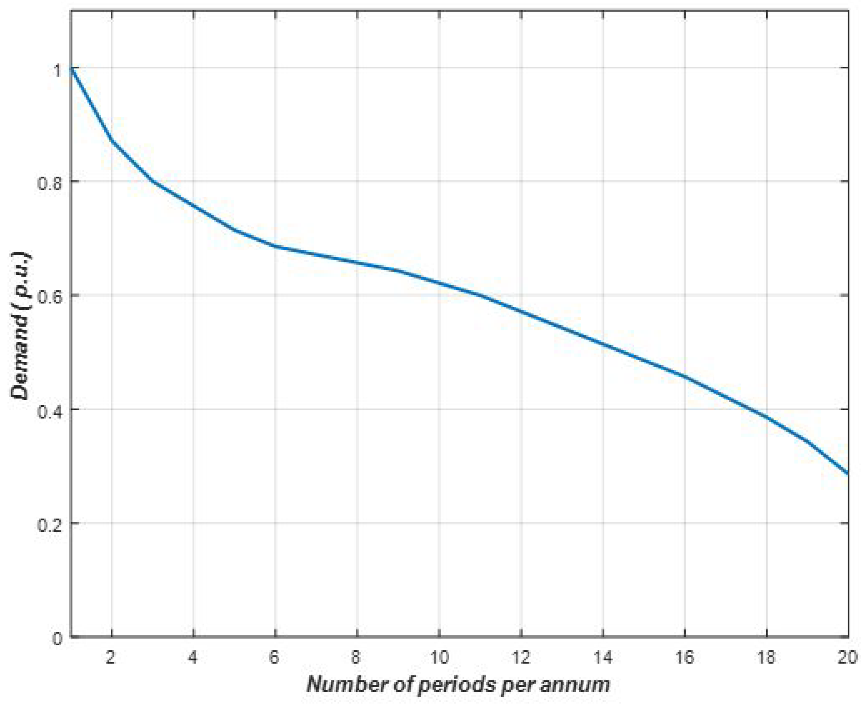
Figure 2.
The 6 bus system’s base year versus planning horizon demand
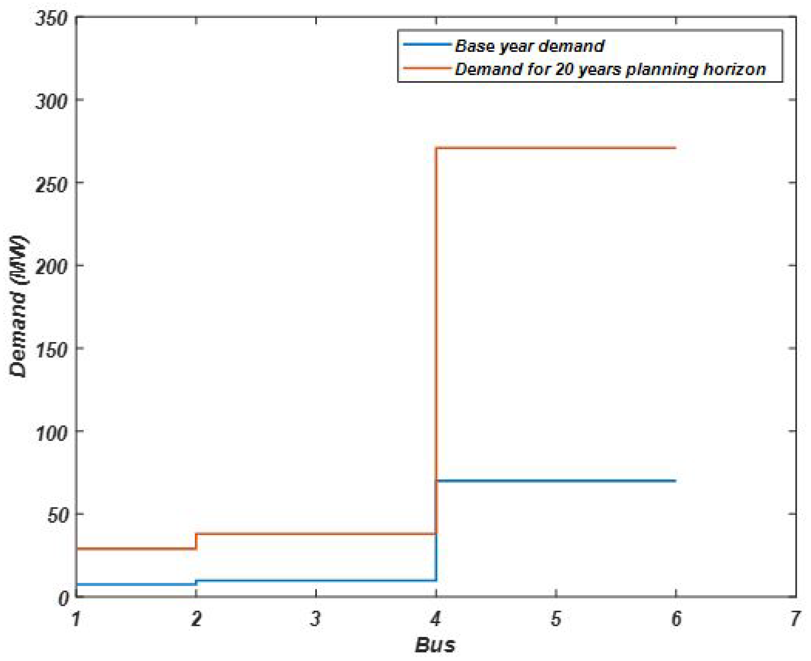
Figure 3.
The 9 bus system’s base demand versus the increased in demand over the planning period
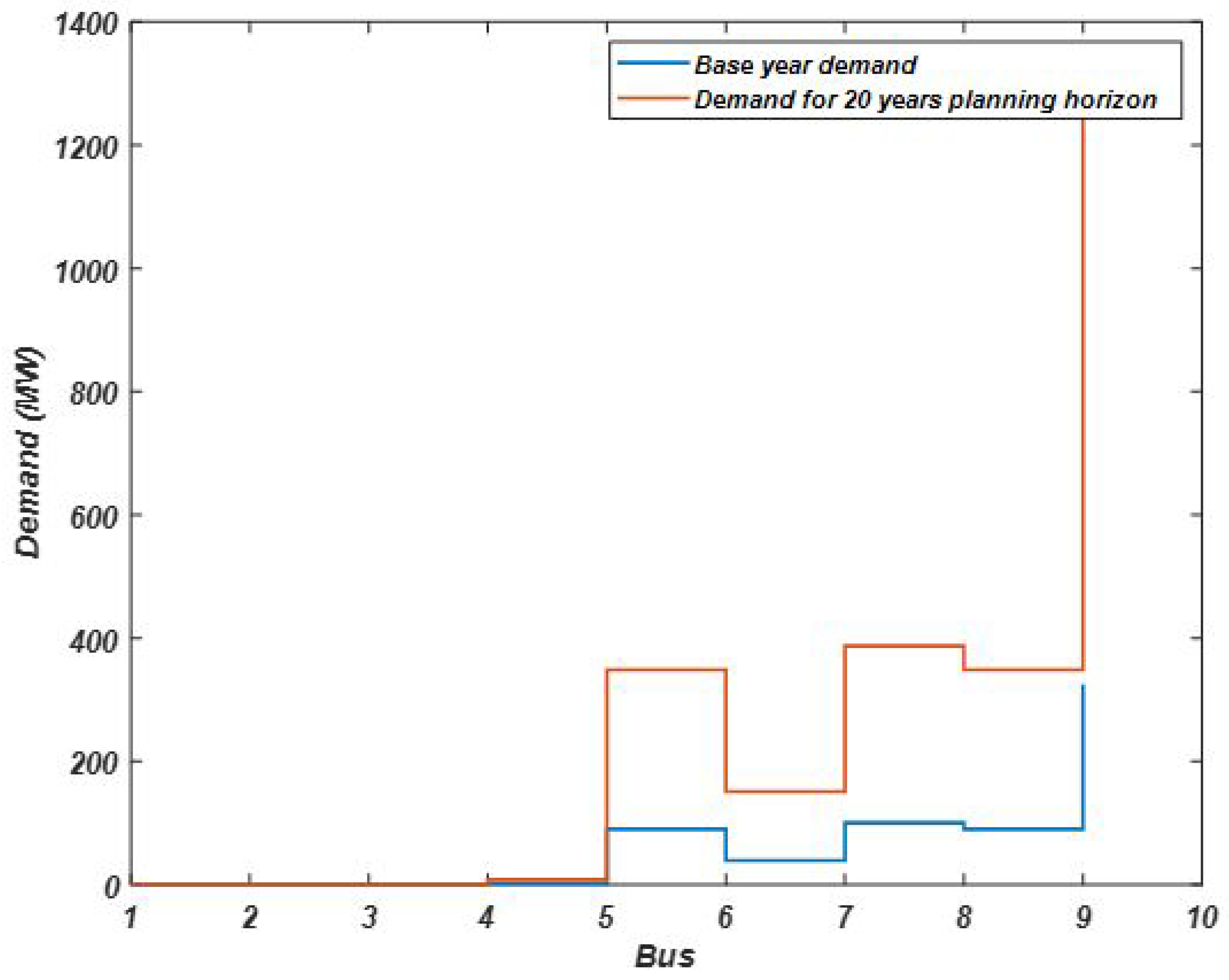
Figure 4.
The 24 bus system’s base year versus planning horizon demands
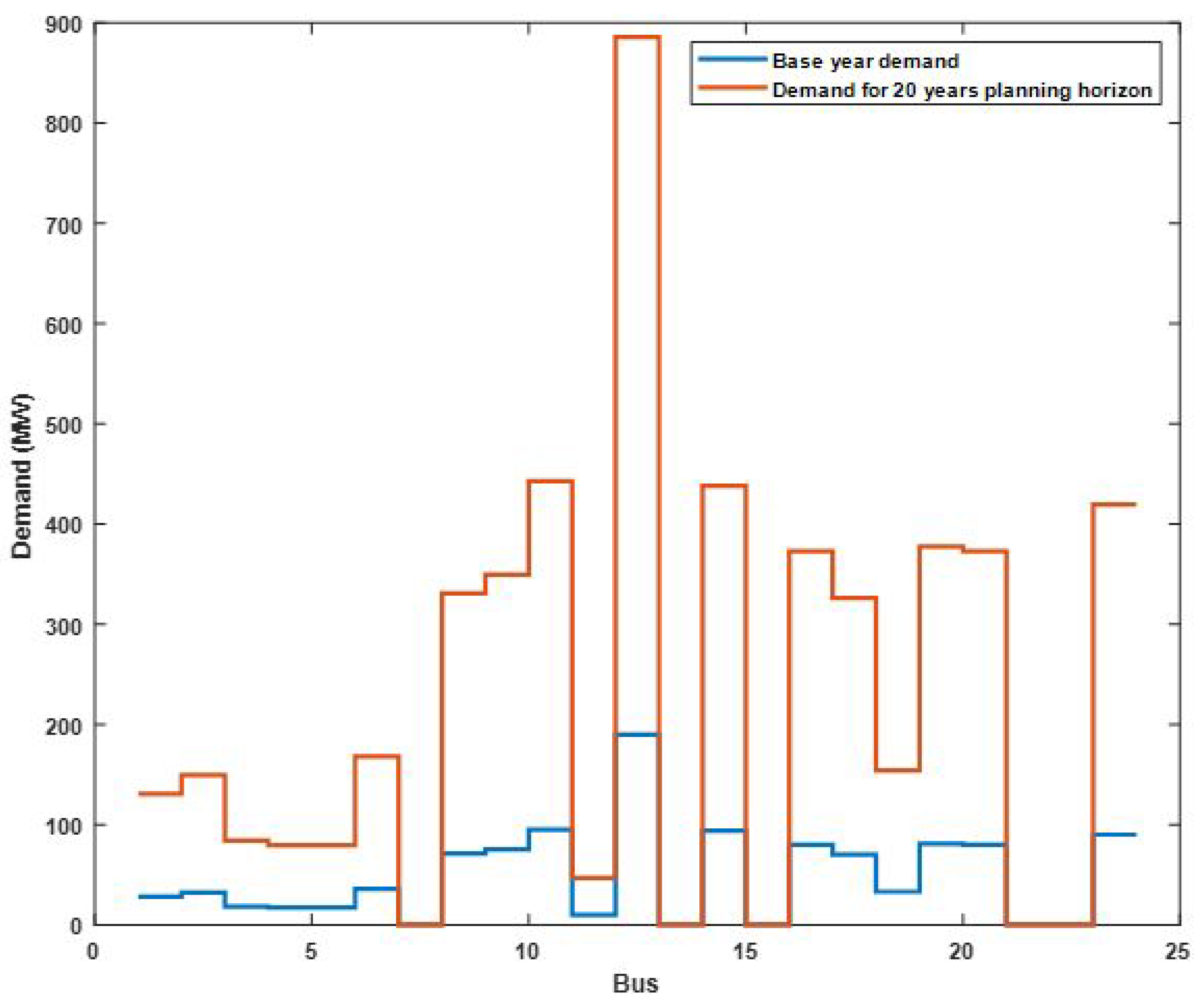
Figure 5.
The 39 bus system’s base year versus planning horizon demands
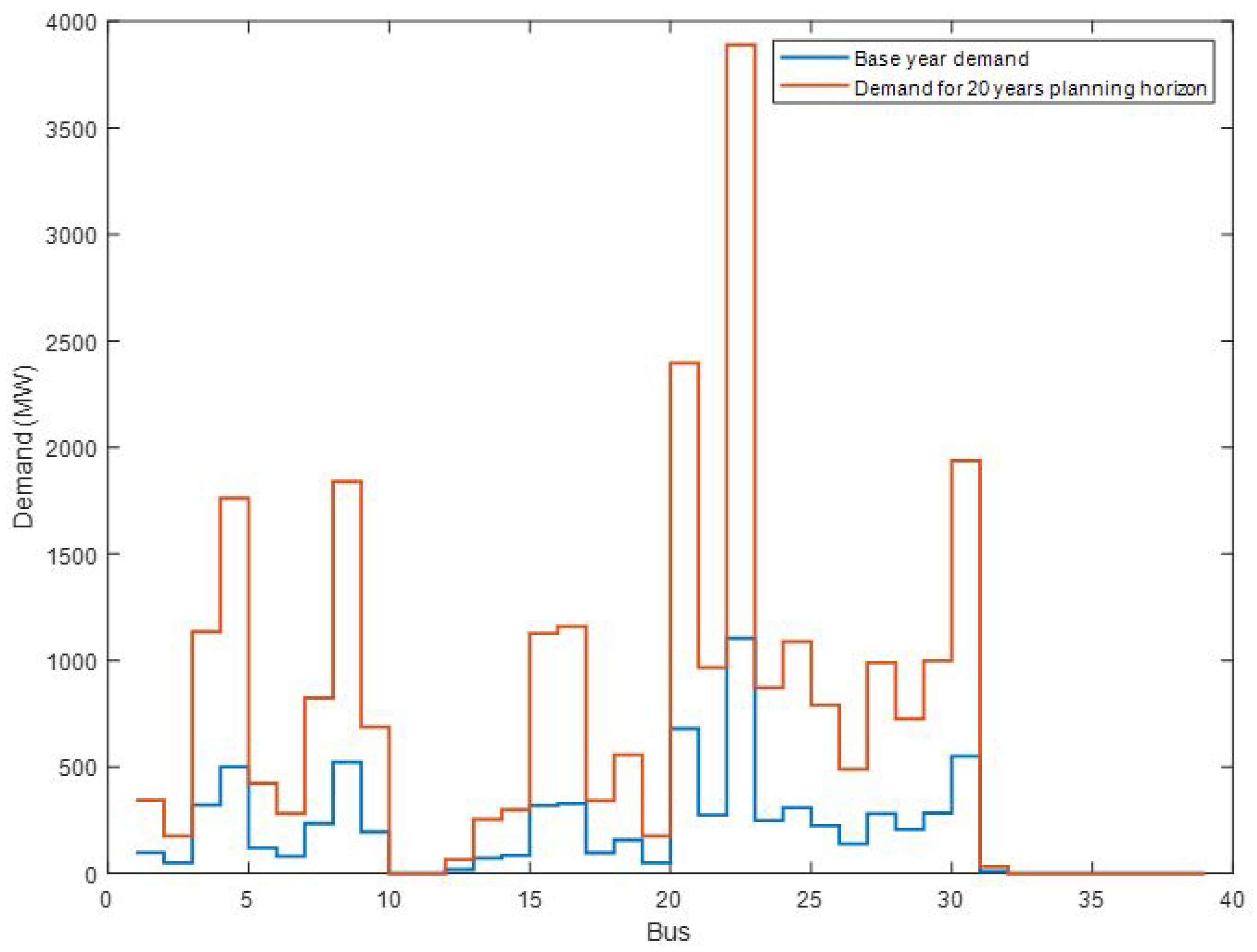
Figure 6.
The 200 bus system’s base year versus planning horizon demands
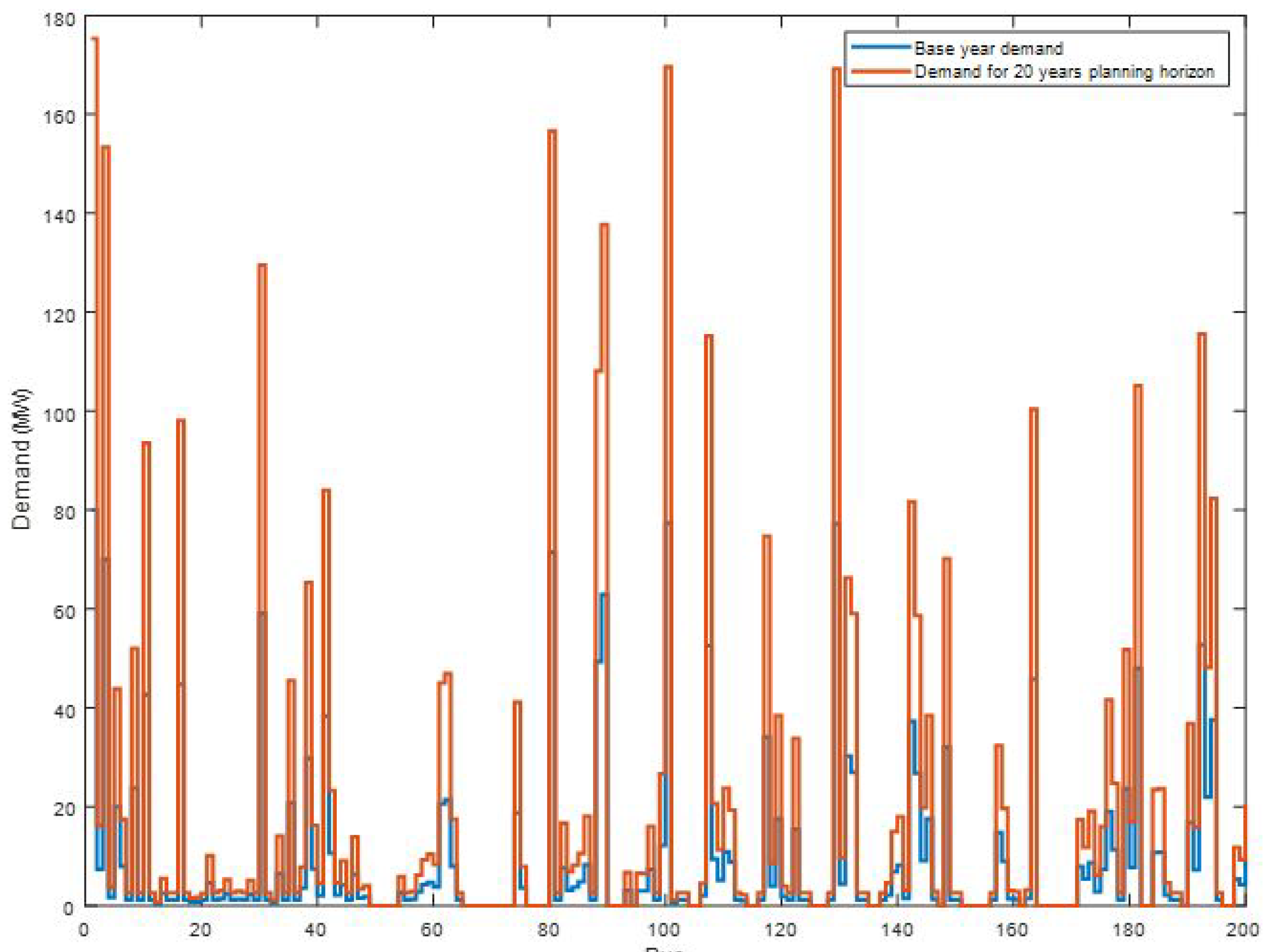
Table 1.
The summary of the TNEP Matrix Model.
| b | ||||||||
|---|---|---|---|---|---|---|---|---|
| 0 | 0 | 0 | 0 | |||||
| 0 | 0 | 0 | 0 | 0 | 0 | 0 | ||
| 0 | 0 | 0 | 0 | 0 | 0 | 0 | ||
| 0 | 0 | 0 | 0 | 0 | 0 | 0 | ||
| M | 0 | 0 | 0 | 0 | 0 | M | ||
| M | 0 | 0 | 0 | 0 | 0 | M | ||
| 0 | 0 | 0 | 0 | 0 | 0 | 0 | ||
| 0 | 0 | 0 | 0 | 0 | 0 | 0 |
Table 2.
The optimal results of the line expansions of the IEEE 6 bus system’s expansion over the planning horizon
Table 2.
The optimal results of the line expansions of the IEEE 6 bus system’s expansion over the planning horizon
| fb-tb | OPF () | New Lines | New Corridors |
|---|---|---|---|
| 2-5 | 14.81 | 1 | - |
| 5-4 | 3.29 | - | 1 |
Table 3.
The optimal generation capacities in the IEEE 6 bus system over the planning horizon
| Bus | MGC () | ||
|---|---|---|---|
| 1 | 155.84 | - | 200 |
| 2 | - | 101.66 | 200 |
| 3 | - | 150 | 150 |
| 4 | 150 | - | 150 |
| 5 | 180 | - | 180 |
| 6 | - | 180 | 180 |
Table 4.
The optimal results of line expansions of the IEEE 9 bus system’s expansion over the planning period
Table 4.
The optimal results of line expansions of the IEEE 9 bus system’s expansion over the planning period
| fb-tb | OPF () | New Lines | New Corridors |
|---|---|---|---|
| 4-9 | 245.76 | 1 | - |
| 4-9 | 129.75 | 1 | - |
| 6-7 | 142.93 | 1 | - |
| 6-1 | 110.28 | - | 1 |
Table 5.
The optimal generation capacities in the IEEE 9 bus system over the planning horizon
| Bus No | MGC () | ||
|---|---|---|---|
| 4 | - | 700 | 700 |
| 5 | - | 300 | 300 |
| 6 | 659.82 | - | 700 |
| 7 | - | 270 | 270 |
| 8 | 300 | - | 300 |
| 9 | 270 | - | 270 |
Table 6.
The optimal results of line expansions of the IEEE 24 bus system’s expansion over the planning horizon
Table 6.
The optimal results of line expansions of the IEEE 24 bus system’s expansion over the planning horizon
| fb-tb | OPF () | New Lines | New Corridors |
|---|---|---|---|
| 7-8 | 245.76 | 2 | - |
| 13-12 | 500 | 1 | - |
| 15-1 | 175 | - | 1 |
| 16-19 | 464.16 | 1 | - |
Table 7.
The optimal generation capacities in the IEEE 24 bus system over the planning horizon
| Bus | MGC () | Bus | MGC () | ||
|---|---|---|---|---|---|
| 1 | 24.39 | 980 | 16 | 980 | 980 |
| 2 | 596.42 | 1000 | 21 | 704.79 | 1002 |
| 7 | 525 | 1002 | 22 | 929.83 | 1970 |
| 13 | 1602.3 | 1970 | - | - | - |
| 15 | 263.06 | 1112 | - | - | - |
Table 8.
The optimal generation capacities in the IEEE 39 bus system over the planning horizon
| Bus | MGC () | Bus | MGC () | ||
|---|---|---|---|---|---|
| 30 | 2557.9 | 3120 | 3 | 1793.5 | 2175 |
| 33 | 1800 | 1956 | 4 | 1956 | 1956 |
| 34 | 1524 | 1524 | 10 | 70.57 | 1524 |
| 35 | 2061 | 2061 | 11 | 1577.9 | 2061 |
| 36 | 1425.9 | 1740 | 24 | 1740 | 1740 |
| 37 | 900 | 1692 | 26 | 1692 | 1692 |
| 38 | 1200 | 2595 | 27 | 2121.5 | 2595 |
| 39 | 2098.5 | 3300 | 31 | 1832.4 | 2033.61 |
Table 9.
The optimal generation capacities in the IEEE 200 bus system
| Bus | MGC () | Bus | MGC () | ||
|---|---|---|---|---|---|
| 49 | 19.93 | 19.93 | 65 | 19.93 | 19.93 |
| 50 | 19.93 | 19.93 | 104 | 19.93 | 19.93 |
| 51 | 19.93 | 19.93 | 105 | 19.93 | 19.93 |
| 52 | 19.93 | 19.93 | 114 | 19.93 | 19.93 |
| 53 | 35.3 | 39.91 | 115 | 39.91 | 39.91 |
| 67 | 60 | 380.6 | 147 | 261.2 | 380.6 |
| 68 | 20.10 | 20.68 | 151 | 20.68 | 20.68 |
| 69 | 70.50 | 122.85 | 152 | 100 | 122.85 |
| 70 | 70.50 | 122.85 | 153 | 100 | 122.85 |
| 71 | 68 | 122.85 | 154 | 122.85 | 122.85 |
| 72 | 68 | 122.85 | 155 | 122.85 | 122.85 |
| 73 | 65 | 122.85 | 161 | 122.85 | 122.85 |
| 76 | 48.6 | 122.85 | 164 | 116.2 | 122.85 |
| 77 | 14.8 | 17.6 | 165 | 17.6 | 17.6 |
| 78 | 10.56 | 10.56 | 166 | 10.56 | 10.56 |
| 70 | 79.2 | 79.2 | 167 | 79.2 | 79.2 |
| 90 | 17.2 | 79.2 | 168 | 79.2 | 79.2 |
| 91 | 14.08 | 14.08 | 169 | 14.08 | 14.08 |
| 92 | 22 | 22 | 170 | 22 | 22 |
| 125 | 79.2 | 79.2 | 182 | 27.68 | 27.68 |
| 126 | 297.44 | 297.44 | 183 | 79.2 | 79.2 |
| 127 | 363.84 | 681.12 | 189 | 297.44 | 297.44 |
| 135 | 6.16 | 6.16 | 196 | 175.4 | 681.12 |
| 136 | 587.4 | 587.4 | 197 | 6.16 | 6.16 |
Disclaimer/Publisher’s Note: The statements, opinions and data contained in all publications are solely those of the individual author(s) and contributor(s) and not of MDPI and/or the editor(s). MDPI and/or the editor(s) disclaim responsibility for any injury to people or property resulting from any ideas, methods, instructions or products referred to in the content. |
© 2020 by the authors. Licensee MDPI, Basel, Switzerland. This article is an open access article distributed under the terms and conditions of the Creative Commons Attribution (CC BY) license (https://creativecommons.org/licenses/by/4.0/).
Copyright: This open access article is published under a Creative Commons CC BY 4.0 license, which permit the free download, distribution, and reuse, provided that the author and preprint are cited in any reuse.


