
Submitted:
21 May 2025
Posted:
22 May 2025
You are already at the latest version
Abstract
In our previous work (i.e., Ref. [14]), we proposed a special Lorentz violation model, which is characterized by that the maximum energy of a particle with mass is finite and proportional to its rest mass rather than infinite predicted by the Lorentz model. In this paper, we continue to investigate the impact of the Lorentz violation model on the curved spacetime. Firstly, we proposed a method for obtaining the spacetime metric without external fields corresponding to this Lorentz violation model. Then, we used this new metric to analyze the proper acceleration of a particle fixed in the Schwarzschild spacetime. To our surprise, we found that when the particle is less than a certain distance from the event horizon of the Schwarzschild black hole, the closer it is to the event horizon, the smaller its proper acceleration becomes, and the proper acceleration drops to 0 when reaching the event horizon. By analogy with the quark model in particle physics, we can also call this phenomenon the ''asymptotic freedom'' in Schwarzschild spacetime, which shows us a different black hole.
Keywords:
Lorentz violation model
; Schwarzschild spacetime
; asymptotic freedom
; black hole
1. Introduction
The study of Lorentz symmetry breaking is a hot topic in current fundamental physics, which is mainly driven by the quantum gravity[1,2,3,4], such as the well-known string theory, and which is also proposed as a possible solution to some difficult problems in black hole. There are many kinds of Lorentz violation models that have been proposed in the literature, among which the most typical and widely discussed Lorentz violation model is the double special relativity model (DSR model), which introduces another constant called “maximum energy or minimum length”[5,6] besides the speed of light. The DSR model is usually expressed as , where Lp denotes the “Planck length”, α is a positive integer and is a real number[7]. Many researchers have investigated the DSR model and demonstrated its ability to solve some challenging problems in the ultra-high energy field[7,8,9,10,11,12]. However, the DSR model is not concise enough that it contains many undetermined parameters, and the physical meaning of these parameters is not very clear[13]. For this reason, in Ref. [14] we proposed another possible Lorentz violation model, which contains only one parameter in the dispersion relation equation of particles. The most remarkable feature of the Lorentz violation model proposed in Ref. [14] is that it naturally returns to the Lorentz model at low and medium energy scale, but when the velocity of the particle is close to c the energy of the particle tends to a limited value (which is similar to the DSR model), rather than infinite predicted by the Lorentz model. In order to clarify the purpose and viewpoint of this paper, here we first briefly review the Lorentz violation model proposed in Ref. [14].
As one knows in special and general relativity that the speed of light occupies a central status, so for most Lorentz violation models, the (local) speed of light is assumed to be variable. In this context, in order to allow it is possible that the (local) speed of light can change between inertial systems, in Ref. [14] it starts from a discussion of a general relationship between the speed of light and the light source, i.e., it assumed that the speed of light observed by an observer moving with a velocity v relative to the light source is nc, where n is dimensionless and variable or invariable. Obviously, due to the fact that many experiments at low or medium energy scale have verified the theory of special relativity and general relativity, there must be some constraints on n, that is, n(v,c)=n(-v,c)=n(v,-c)=n(-v,-c) and n(v=0, c)=1 (The detailed reasons for this constraints can be seen in Ref. [14]). The above assumption can be expressed in the following equations
where (x, y, z, t) corresponds to the inertial system S, and (x’, y’, z’, t’) corresponds to the inertial system S’, and here for simplicity, we assume that the three spatial coordinates of the two coordinate systems are parallel to each other, and the direction of v (i.e., the relative velocity between the two inertial systems) is along the x-axis or x’-axis. The first formula of Eq. (1) represents that the light source is fixed in S, so for observer in S, the observed speed of light is c, which corresponds to that n(v=0, c)=1, while for the observer in S’, the observed speed of light is nc. Similarly, since S and S’ are equivalent, when the light source is fixed in S’, so for observer in S’, the observed speed of light is c, while for the observer in S, the observed speed of light is nc, which corresponds to the second formula of Eq. (1).
From Eq. (1), the coordinate transformation between the two inertial systems moving relative to each other with velocity v can be obtained
where, . And n satisfies n(v,c)= n(-v,c)=n(v,-c)=n(-v,-c) and n(v=0, c)=1.
From Eq. (2) one can obtain that if dx/dt=c, then dx’/dt’=nc, and if dx’/dt’=c, then dx/dt=nc, which in turn indicates that Eq. (2) is the solution of Eq. (1), and more importantly, it shows again that the two inertial systems are equivalent.
Eq. (2) is highly similar in form to the Lorentz transformation (i.e., replacing c with k in the Lorentz transformation yields Eq. (2)), and it has been shown in Ref. [14] that Maxwell’s equations are also covariant based on Eq. (2). At the same time, the dispersion relation of particles with rest mass m0, and the spacetime metric, compared to the form as in the Lorentz model, are modified accordingly as
Where E0=m0k2, E=γm0k2 denotes the particle’s total energy, p=γm0v denotes the particle’s momentum, and γ=γ(v,c), k=k(v,c). (T, X, Y, Z) denotes the coordinates of inertial system.
So next we have a question, what is the expression for n? Obviously, if n≡1, then Eq. (2) returns to the Lorentz transformation. However, we notice that if n takes the following expression, then when v is close to c, the total energy of the particle will be finite rather than infinite predicted by the Lorentz model
Where Q is a constant and its value needs to be determined by the experiment. As mentioned in Ref. [14], we do not yet know the concrete value of Q because the current experimental energy is not high enough, but it can be known from a large number of existing experimental results that Q≈0.
Here we can re-draw the curve of n~v as in Figure 1.
n-1 can be viewed as the degree to which the speed of light observed by the observer in an inertial systems moving relative to the light source deviates from c. As can be seen from Figure 1 that n is very close to 1 over a large range of v. And it is because of this property of n that Eqs. (2)~(4) does not violate a large number of existing experimental results conducted at low or medium energy scale. In fact, the smaller the value of Q is, the higher the energy at which Eqs. (2)~(4) deviates significantly from the Lorentz model, and when Q=0, , then correspondingly, Eqs. (2)~(4) return to the case as in the Lorentz model.
Thus, based on Eq. (5), both the time-space scaling factor γ and the particle’s total energy E have a limit,
This is just the purpose the Lorentz violation model proposed in Ref. [14] that it makes the total energy of particles have a limit rather than infinite predicted by the Lorentz model as v approaches c. But the energy limit in Ref. [14] is different from which assumed in the DSR model, which considers the total energy limit of different particles to be a constant (which often be referred to the Planck energy or near Planck energy), while here as shown in Eq. (6), the total energy limit of a particle is proportional to its rest mass.
Above we briefly reviewed the model in Ref. [14], all of which were discussed are on the basis of inertial systems. So, what impact will this Lorentz violation model have on the curved spacetime? It is the issue that this paper aims to discuss.
2. Einstein Turntable
Let us first discuss the simple and famous case called Einstein turntable. It is well known that Einstein turntable presents a non-Euclidean geometry structure (i.e., Lobachevsky geometry), and its spacetime metric is [15]
Now we can follow the derivation process of Eq. (7) corresponding to the Lorentz model to derive the spacetime metric of Einstein turntable corresponding to Eq. (2).
For a turntable rotating at a constant speed ω, we can assume that the acceleration system xμ =(ct, r, θ, z) on the turntable and the inertia system Xμ =(cT, X, Y, Z) at the center of the turntable have the following relationship
Substituting Eq. (8) into Eq. (4) we can obtain
where v in k denotes the proper velocity and v=ωr.
It can be seen from Eq. (7) that when ωr →c, then g00→0, while for Eq. (9), when ωr →c, then g00→(1-Q)/[2log(Q)-Q+1]. In addition, it can be derived from Eq. (7) that the proper acceleration of a particle fixed in the spacetime is a0=ω2r/(c2-ω2r2), for which when ωr →c, then a0 tends to be infinite. While for Eq. (9), we can obtain that when ωr →c, a0 tends the following value
Eq. (10) shows us that for Eq. (2), when Q is not equal to 0 (Q=0 corresponds to the Lorentz model), the proper acceleration in Einstein turntable can be avoided from being infinite, which is mathematically singular.
Above, we can see that when Q is not equal to 0, a phenomenon different from which predicted by the Lorentz model will occur. Then, what impact will it have on the classical Schwarzschild spacetime? Obviously, the most important thing here is to obtain the Schwarzschild spacetime metric corresponding to Eq. (2). Next, we will first introduce a method for obtaining this new spacetime metric.
3. A Method for Obtaining the Spacetime Metric
As we know, Minkowski spacetime corresponding to the Lorentz model is a four-dimensional spacetime. While, in Eq. (4) it adds a scaling factor k into the time dimension of the Minkowski spacetime metric, then, mathematically, we can equivalently view Eq. (4) as a cross-section equation in a five-dimensional spacetime, where, similar to the four-dimensional spacetime expression, the five-dimensional spacetime is expressed as
Where ζ is the fifth dimension, and the fifth dimension is equal to the other four dimensions. And we know that if we take a cross-section in the above five-dimensional spacetime that deviates from the plane formed by the origin and (T, X, Y, Z) by an angle θ, and is parallel to the axis (X, Y, Z) at the same time (here, for a better understanding, one can also regard this five-dimensional space-time as a three-dimensional space-time, and the three coordinate axes of the three-dimensional space-time are (icT, X, ζ), then the above-mentioned special cross-section passes through the origin and the X-axis, and deviates from the plane XOT by an angle θ), then the intersection equation of this cross-section with the five-dimensional spacetime is
Substituting the second formula of Eq. (12) into its first formula, it has
Comparing Eq. (13) with Eq. (4) we can obtain that 1+tan2θ=k2. And if we substitutes the expression of n into k2 we will obtain that k2∈[1, 2ln(Q)/[2ln(Q)-Q+1]], which means the solution of θ is a real number. Due to Q~0, it means θ~0. And due to k2 is not a constant, it means the above cross-section is not a constant one but varies with the velocity of the inertial system. In addition, due to the cross-section is parallel to the axis (X, Y, Z), the spatial part of Eq. (4) is the same as which in the Minkowski metric.
Here we propose a method for obtaining the spacetime metric corresponding to Eq. (2), that is, extending the four-dimensional spacetime corresponding to the Lorentz model into the five-dimensional spacetime, and then obtaining a special cross-section equation of this five-dimensional spacetime (So the cross-section is four-dimensional). So next we will use this method to obtain the Schwarzschild spacetime metric corresponding to Eq. (2). Here it should be noted that the five-dimensional spacetime proposed in this section may be merely an equivalent approach in mathematics and has nothing to do with the real world.
4. A Different Schwarzschild Space-Time
As we know the outer metric corresponding to the Schwarzschild space-time in the framework of Lorentz model is [15]
The above expression is presented in a cylindrical coordinate system (r, θ, φ). And it can be also presented in a rectangular coordinate system (x, y, z)
Now our goal is to obtain the Schwarzschild spacetime metric corresponding to Eq. (2). First using the method in Sect. 3, we extend Eq.(15) into the five-dimensional spacetime in the way of equalizing all coordinates
where r=(x2+y2+z2+ζ2)1/2.
Second, we will take a special cross-section in the above five-dimensional spacetime. Noting that the cross-section is parallel to the axis (X, Y, Z), that is, the part related to spatial coordinates in the new metric corresponding to Eq.(2) is the same as the spatial part in the original metric corresponding to the Lorentz model, then based on Eq. (12), the corresponding spacetime metric will be
where , , and here v is the proper velocity of an object moving freely along geodesics in the radial direction, and for the Schwarzschild space-time, .
Based on Eq. (17) we can obtain the proper acceleration a0 of an object fixed in the spacetime. However, its expression is rather long and we will not list it here (Some computing software, such as MATLAB, can help us do these calculations). But we find that, based on the obtained proper acceleration, there is
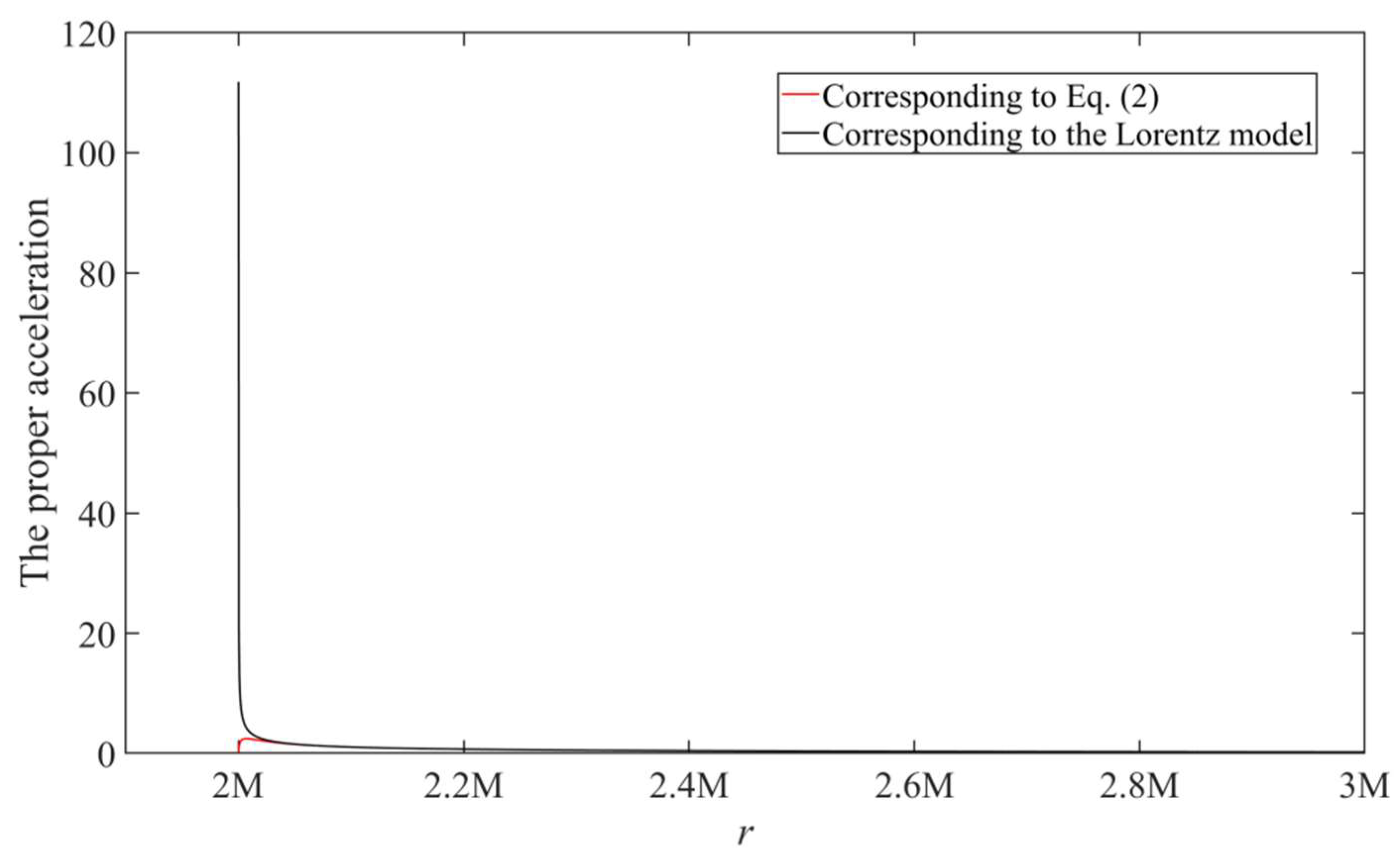
Eq. (18) shows us that when an object is fixed at the event horizon of the Schwarzschild black hole (the location of the event horizon corresponds to the solution of g11=1-2M/r=0, and its solution is r=2M), surprisingly, its proper acceleration is 0. This conclusion is quite different from which predicted by the Lorentz model or general relativity. In general relativity, the proper acceleration of the above object is , which means when r→2M, the proper acceleration tends to be infinite. And Figure 2 shows a comparison between the two results, where Q is taken as as in Figure 1.
Eq. (18) and Figure 2 implies that it is possible that an object remain stationary at the event horizon, which will undoubtedly have a significant impact on the black hole dynamics or thermodynamics at present, and for the black hole thermodynamics we will discuss it in the following article.
5. Summary
In this paper, we extend the study of a special Lorentz violation model proposed in Ref. [14] into curved spacetime, namely the classical Schwarzschild spacetime. In order to obtain the Schwarzschild spacetime metric corresponding to the Lorentz violation model, we propose a method of five-dimensional spacetime, and the four-dimensional spacetime metric we require is a special cross-section of the five-dimensional spacetime. According to this method, we obtained a new Schwarzschild spacetime metric. Then we analyzed the proper acceleration of an object fixed in the Schwarzschild spacetime and were surprised to find that when the object approaches the event horizon of the Schwarzschild black hole, the gravitational force it subjected to suddenly approaches zero, rather than approaching infinity as predicted by the Lorentz model or general relativity. This phenomenon is somewhat similar to the quark model in particle physics, and we can also refer to it as the ‘’asymptotic freedom’’ in black hole.
It should be noted that in this paper, the new Schwarzschild spacetime metric corresponding to Eq. (2) is directly derived from the usual Schwarzschild spacetime metric. This method is only applicable when there is no external field (for example, the energy-momentum tensor of vacuum field without considering cosmological constants is 0), while when there exists an external field, such as the Kerr-Newman metric corresponds to a non-zero energy-momentum tensor (i.e., the electromagnetic field), then it is not applicable. This is because when there exists an external field, the energy-momentum tensor of external field will should be modified at ultrahigh energy scale based on Eq. (2), thus leading to the modification of the usual spacetime metric. In other words, we need to first modify the external field at ultrahigh-energy scale, then with which obtain the corresponding spacetime metric using the Einstein field equation, and further obtain the new spacetime metric corresponding to Eq. (2) base on the method in Sect. 3. Therefore, this paper temporarily only discusses the simple Einstein turntable (in fact, the modified form of the Einstein turntable metric corresponding to Eq. (2) can also be obtained using the method in Sect. 3) and the typical and famous Schwarzschild spacetime metric, as neither of them has an external field.
In our previous paper, it has been shown that a non-zero value of Q can avoid infinity in certain cases [14,16], and this paper once again shows that a non-zero value of Q can avoid infinity in Schwarzschild black hole. It should be emphasized again that if Q=0, the Lorentz violation model mentioned in this paper will return to the Lorentz model. However, since the energy our current experiments conducted is still not high enough to measure the value of Q, but a very small and non-zero value of Q can indeed help solve some problems that are difficult to understand in today’s physics.
In addition, From Eq. (10) and Eq. (18), it can be seen that since there is no infinity when v=c (i.e., r=1/ω in Einstein turntable and r=2M in Schwarzschild spacetime), what will happen when v>c? Unfortunately, we don’t know here either. This is mainly because we don’t know what the expression of n is when v>c. If the expression of n is still the same as Eq. (5), then the interior of the event horizon will be a completely different from which predicted by the Lorentz model. However, currently there is no experiment or theory to tell us what the expression of n may be like when v>c. Therefore, this article does not discuss the phenomena within the event horizon of the Schwarzschild black hole.
Data Availability Statement
No Data associated in the manuscript.
References
- Han, M.X.; Huang, W.M.; Ma, Y.G. Fundamental structure of loop quantum gravity. International Journal of Modern Physics D 2007, 16, 1397–1474. [Google Scholar] [CrossRef]
- Ashtekar, A.; Lewandowski, J. Background independent quantum gravity: a status report. Classical and Quantum Gravity 2012, 21, R53–R152. [Google Scholar] [CrossRef]
- Thiemann, T. Modern canonical quantum general relativity. Cambridge University Press: United Kingdom, 2007. [Google Scholar]
- Rovelli, C. Quantum gravity. Cambridge university press: United Kingdom, 2007. [Google Scholar]
- Amelino-Camelia, G. Relativity in space-times with short-distance structure governed by an observer-independent (Planckian) length scale. International Journal of Modern Physics D 2002, 11, 35–59. [Google Scholar] [CrossRef]
- Amelino-Camelia, G. Testable scenario for Relativity with minimum-length. Physics Letters B 2001, 510, 255–263. [Google Scholar] [CrossRef]
- Amelino-Camelia, G. Quantum spacetime phenomenology. Living Reviews in Relativity 2013, 16, 5. [Google Scholar] [CrossRef] [PubMed]
- Kowalski-Glikman, J. Introduction to doubly special relativity. Lecture Notes in Physics 2005, 669, 132–159. [Google Scholar]
- Kostelecky, A. CPT, T, and Lorentz Violation in Neutral-Meson Oscillations. Physical Review D 2001, 64, 407–412. [Google Scholar] [CrossRef]
- Kostelecky, A. Theory and Status of Lorentz Violation. American Physical Society 2008, 132–155. [Google Scholar]
- Girelli, F.; Livine, E.R.; Oriti, D. Deformed special relativity as an effective flat limit of quantum gravity. Nuclear Physics B 2005, 708, 411–433. [Google Scholar] [CrossRef]
- NNilsson, A.; Dabrowski, M.P. Energy scale of lorentz violation in rainbow gravity. arXiv: Cosmology and Nongalactic Astrophysics 2016. [Google Scholar] [CrossRef]
- Ping He, BoQiang Ma. Lorentz symmetry violation of cosmic photons. Universe 2022, 8, 323. [Google Scholar] [CrossRef]
- Jinwen Hu, Huan Hu, A special rainbow function. Result in Physics 2022, 43, 106082. [CrossRef]
- Weinberg, S. Gravitation and Cosmology: Principles and Applications of the General Theory of Relativity. Wiley: New York, 1972. [Google Scholar]
- Jinwen Hu, Huan Hu, Correction to the quantum relation of photons in the Doppler effect based on a special Lorentz violation model. Result in Physics 2024, 64, 107920. [CrossRef]
Figure 1.
The curve of n(v)~v when taking (set c=1). Since here it shows the global picture of the curve, a transition arc at the corner is too small to show [14]. From here or Eq. (5) it can be seen that when v=1, n=0.
Figure 1.
The curve of n(v)~v when taking (set c=1). Since here it shows the global picture of the curve, a transition arc at the corner is too small to show [14]. From here or Eq. (5) it can be seen that when v=1, n=0.
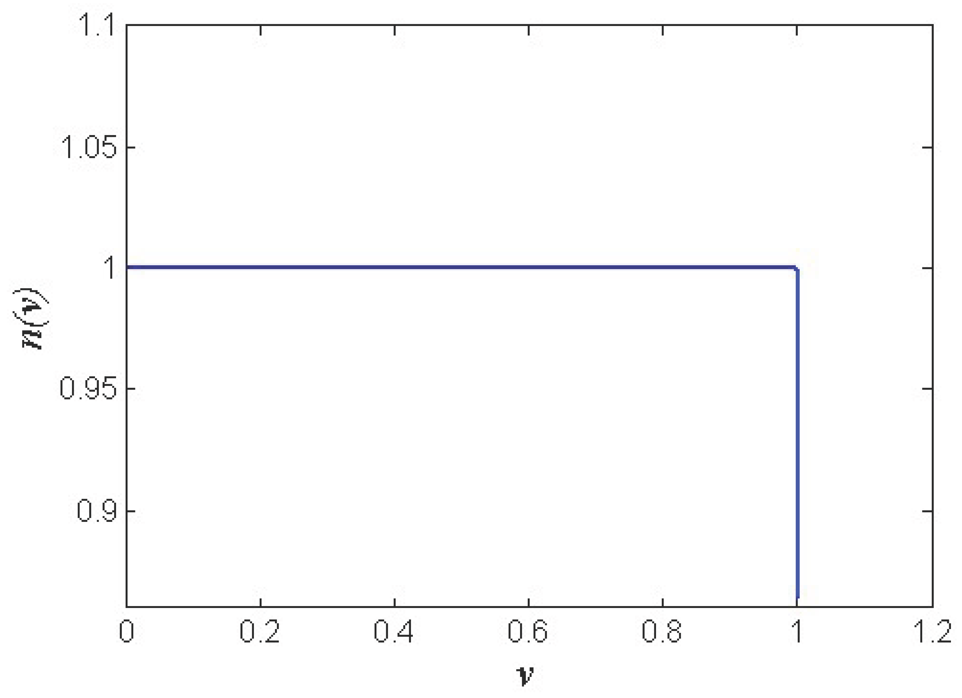
Figure 2.
The comparison of the proper acceleration of an object fixed in Schwarzschild spacetime predicted by Eq. (2) and the Lorentz model. It tend to be infinite at r=2M for the curve predicted by the Lorentz model, while for the curve predicted by Eq. (2), it tends to 0 at r=2M. When r is much greater than 2M, the two curves basically coincide.
Disclaimer/Publisher’s Note: The statements, opinions and data contained in all publications are solely those of the individual author(s) and contributor(s) and not of MDPI and/or the editor(s). MDPI and/or the editor(s) disclaim responsibility for any injury to people or property resulting from any ideas, methods, instructions or products referred to in the content. |
© 2025 by the authors. Licensee MDPI, Basel, Switzerland. This article is an open access article distributed under the terms and conditions of the Creative Commons Attribution (CC BY) license (http://creativecommons.org/licenses/by/4.0/).
Copyright: This open access article is published under a Creative Commons CC BY 4.0 license, which permit the free download, distribution, and reuse, provided that the author and preprint are cited in any reuse.


