
Submitted:
20 May 2025
Posted:
21 May 2025
You are already at the latest version
Abstract
Photovoltaic (PV) modules undergo comprehensive testing to validate their electrical and thermal properties prior to market entry. These evaluations consist of durability and efficiency tests performed under realistic outdoor conditions with natural climatic influences, as well as in controlled laboratory settings. The overall performance of PV cells is affected by several factors, including solar irradiance, operating temperature, installation site parameters, prevailing weather, and shading effects. In the presented study, three distinct PV modules were analyzed using a sophisticated large-scale steady-state solar simulator. The current-voltage (I-V) characteristics of each module were precisely measured and subsequently scrutinized. To augment the analysis, a three-layer artificial neural network, specifically the multilayer perceptron (MLP), was developed. The experimental measurements, along with the outputs derived from the MLP model, served as the foundation for a comprehensive global sensitivity analysis (GSA). The experimental results revealed variances between the manufacturer's declared values and those recorded during testing. The first module achieved a maximum power point that exceeded the manufacturer's specification. Conversely, the second and third modules delivered power values corresponding to only 85-87% and 95-98% of their stated capacities, respectively. The global sensitivity analysis further indicated that while certain parameters, such as efficiency and the ratio of Voc/V, played a dominant role in influencing the power-voltage relationship, another parameter, U, exhibited a comparatively minor effect. These results highlight the significant potential of integrating machine learning techniques into the performance evaluation and predictive analysis of photovoltaic modules.
Keywords:
photovoltaics
; current-voltage characteristics
; solar energy
; machine learning
; neural networks
; statistical modeling
; sensitivity analysis
1. Introduction and State of the Art
Electricity underpins modern economic and technological progress and is deeply integrated into everyday life. As traditional energy resources gradually deplete and environmental concerns intensify, the search for renewable energy alternatives becomes increasingly urgent. Among these alternatives, photovoltaics (PV) stand out as one of the most accessible and scalable solutions for sustainable electricity generation [1]. PV systems, which capture energy from solar photons, are composed of several fundamental components including modules, inverters, batteries, cables, and safety units [2]. The construction of a typical PV module involves multiple layers: an outer glass layer with anti-reflective treatment, one or more encapsulation layers, an array of solar cells, and a back sheet. This layered architecture enables PV systems to serve diverse applications, ranging from small-scale installations powering individual devices to large solar farms generating tens of megawatts of clean energy [3]. PV cell technologies are categorized into three generations based on their underlying materials and stages of market adoption [3].
The first generation involves well-established, wafer-based crystalline silicon technology, which can be further divided into monocrystalline (M-Si) and polycrystalline (P-Si) types. This technology is highly efficient due to the inherent properties of silicon [4,6]. Historical benchmarks include the pioneering silicon solar cell developed by Chapin et al. in 1954 with an initial efficiency of approximately 6%, which has since improved dramatically to values around 26.1% [7,8,9]. The second generation utilizes thin-film approaches such as amorphous silicon, micromorph silicon, cadmium telluride (CdTe), and copper-based technologies (CIS/CIGS). Although these systems offer reduced production costs, their efficiency generally lags behind that of crystalline silicon devices [7,10,11,12,13]. The third generation encompasses emerging technologies such as concentrating photovoltaics (CPV), organic PV cells, and novel concepts including nanowires and quantum dots, which are at various stages of research and demonstration [9,14,15]. Recent reports suggest that some third-generation approaches have reached efficiencies in the vicinity of 18.9% [16]. The efficiency and longevity of PV modules are subjected to various internal and external factors. Internally, the consistency and quality of semiconductor interfaces, the configuration of multiple cell layers, and the inherent material properties directly influence conversion efficiency. Externally, factors such as solar irradiance, ambient temperature, weather conditions, and shading significantly affect output. Even slight increases in module surface temperature can result in measurable drops in performance, studies have shown that a temperature rise can reduce the maximum power output by approximately 0.4-0.5% per degree Celsius [20,22,23,24,29]. In addition to the intrinsic characteristics of the PV modules, the integration of modern cooling technologies has been a subject of extensive research. Approaches such as active cooling using pumps and heat sinks or passive methods involving strategically positioned acrylic sheets have shown potential in mitigating thermal losses, thereby enhancing overall module efficiency [25,26,27,28,30]. Innovative designs not only help maintain optimal operating temperatures but also extend the operational life span of the modules.
The rapid evolution in PV technologies is also mirrored by advancements in artificial intelligence. AI techniques, including artificial neural networks (ANNs) and deep learning models like long short-term memory (LSTM) networks, are increasingly applied to monitor, predict, and optimize the performance of solar energy systems. These methods analyze data collected from sensors, tracking variables such as temperature, solar radiation, humidity, and even particulate accumulation, to forecast future performance and guide maintenance strategies. Recent studies demonstrate that machine learning (ML) and deep learning (DL) models can significantly enhance predictive accuracy, offering more robust solutions in solar energy forecasting when compared to traditional statistical methods [55,56,57,58,59,60,61,62,63,64,65,66,67,68,69,70,71,72,73].
Finally, beyond the technological and operational innovations, the overarching goal remains to integrate renewable energy into existing infrastructures effectively. Achieving a sustainable energy balance demands novel policy frameworks and socio-economic strategies that foster renewable energy adoption while mitigating environmental impacts, a multidisciplinary effort that continues to evolve alongside technological progress. The structure of this discussion reflects an integrated approach: initially outlining the importance of electricity and renewable energy; then detailing PV system structures and technologies across three generations; addressing the influences of environmental and operational factors; and finally, discussing the role of AI in optimizing solar energy systems. This comprehensive perspective aims to contribute novel insights into both the current state and future direction of renewable energy technologies.
2. Materials and Methods
2.1. Testing Methods for PV Modules
The rapid evolution of the photovoltaic industry since the early 2000s has necessitated the establishment of uniform standards and regulations to ensure a consistent certification process for PV modules. In European Union countries, the certification process adheres to the standards set by the International Electrotechnical Commission (IEC). Specifically, IEC 61215 [34] outlines the construction qualification and type approval requirements for photovoltaic modules intended for terrestrial applications that will operate reliably over long periods under the climatic conditions specified by IEC 60721-2-1 [35]. These tests evaluate the performance of the PV modules under standardized conditions, and the standard is applicable to both crystalline silicon and thin-film modules. Within the framework of this work, two principal test methodologies were employed:
- MQT 04 – Measurement of Temperature Coefficients: This test involves quantifying the temperature coefficients of current, voltage, and peak power in accordance with PN-EN 60904-10 [34]. It aims to determine how the electrical parameters of PV modules vary with temperature, and it requires a device specifically designed to control the module’s temperature during measurement.
- MQT 06 – Performance under STC and NOCT Conditions: This evaluation focuses on determining the electrical performance of the module under Standard Test Conditions (STC) and under NOCT (Nominal Operating Cell Temperature) conditions. The STC measurement is used to verify the module's nameplate specifications and should be conducted with either natural solar radiation or a solar simulator of BBA-class quality, or better [34].
2.2. Characteristics of the Tested PV Modules
The first module evaluated is a double-sided, monocrystalline module, referred to as “Module 1”. According to the manufacturer’s documentation, the module exhibits an efficiency of 20% and a maximum power output of 365 Watts. Moreover, the manufacturer offers a 30-year warranty on the additional linear power output, which is expected to retain approximately 85% of its initial performance after 30 years [36].
The second module examined is a CIGS thin-film module, designated as “Module 2”. This module exhibits an efficiency of approximately 13% and is capable of producing a maximum power output of 145 W. It features a double-glazed panel design which minimizes the risk of micro-cracking and thereby enhances the module’s overall durability. The manufacturer guarantees that the module will retain at least 80% of its rated power after a period of 25 years [37].
The third module analyzed is a monocrystalline single-sided photovoltaic module, referred to as “Module 3”. This module achieves an efficiency of about 19.3% and can deliver a maximum power of 315 watts. The developer ensures that the degradation rate of the module remains constant over a 25-year period [38]. For a detailed comparison, the characteristics of all tested modules are summarized in Table 1.
2.3. Experimental Description and Test Methods
The experiments were carried out using a stationary, steady-state solar simulator, Class AAA (see Figure 1), designed for measuring the performance of photovoltaic modules under tightly controlled test parameters. This device precisely replicates solar radiation according to specified conditions, enabling the measurement of the maximum power output of each photovoltaic module under standard test conditions. For each module, tests were repeated five times, and the results were averaged to estimate the performance. All PV modules tested were brand-new, meaning they had never been previously used (see Figure 2).
The measurement setup comprises a large-area, stationary steady-state solar simulator combined with a system for analyzing the current-voltage characteristics of the photovoltaic modules, along with a calibrated, accredited reference coil. The reference coil, positioned on the module under test, was utilized to obtain baseline measurements that were subsequently compared with the readings from the module itself [39].
Both the MQT 06 and MQT 04 evaluations were performed using a large-area, stationary steady-state solar simulator. For the MQT 06 procedure, the PV module’s electrical parameters were recorded under Standard Test Conditions (STC), defined by a solar irradiance of (1000 ± 100) W/m² and an ambient cell temperature of (25 ± 2) °C. The module, fitted with a calibrated reference coil, was slid into position beneath the simulator’s lamp array prior to initiating each measurement.
In the MQT 04 sequence, ten independent readings were taken per module: five measurements were adjusted to a reference temperature of 25 °C, while the other five were left uncorrected. Module temperatures were logged immediately before and after each test run to ensure accuracy of the temperature-dependent correction.
A pivotal aspect of this work was constructing machine learning models to quantify and select the most impactful correlations among independent variables for numerical simulations based on the experimental dataset. The correlation coefficient, Rij, spans from -1 to +1, where positive values indicate that an increase in variable i leads to an increase in variable j, and negative values imply an inverse relationship. To capture nonlinear dependencies, we applied Spearman’s rank correlation coefficient (ρ), which is particularly suited for assessing monotonic, nonparametric associations [40].
Within the multilayer perceptron (MLP) framework applied here, each incoming feature xi at the input layer is scaled by its corresponding synaptic weight wij, as illustrated in Figure 3. The sum of these weighted inputs is then passed through an activation function f which may be linear or one of several nonlinear forms (e.g., exponential, hyperbolic tangent, sine, or logistic) before being delivered to the output neurons. During training, the values of wij are iteratively adjusted using numerical optimization techniques designed to minimize the mean squared error (MSE) between the network’s predictions and the true targets [41]:
where is the ground truth for the -th training data point, is the corresponding output from the neural network, , and is the number of data points in the training set.
Each coordinate of the output was calculated according to the following formula:
where: - the number of inputs to the model, - the number of neurons in the hidden layer, - the values of weights between the inputs and the neurons of the hidden layer, – neuron loads of the hidden layer, - the values of weights between neurons of the hidden layer and neuron of the output layer, - the activation function. At the stage of creating the MLP model, it is crucial to determine the number of neurons in the hidden layer. Widely accepted guidelines specify that the hidden layer neuron count J should satisfy j ≤ J ≤ 2 j + 1, where j denotes the number of explanatory variables [42]. To avoid overfitting of the model, Rogers and Dowl [43] suggested that the value of should not be less than (where is the number of data observations in the learning set). The number of neurons in the hidden layer can also be determined by trial and error method minimizing the prediction error, but not allowing overlearning of the model (when with an increase in the prediction error increases, there is a decrease in the generalization ability of the model). In this study, a three-layer neural network was implemented, taking as inputs the current-voltage characteristics of each PV module and yielding two outputs corresponding to the module’s power-voltage curves. The dataset was partitioned into training (70 %), testing (15%), and validation (15%) subsets.
Simultaneously, a global sensitivity analysis was carried out to pinpoint which parameters most strongly influence the power-voltage relationship, with sensitivity coefficients computed to quantify each factor’s impact. To quantify the agreement between the true value for each coordinate of the m-th validation sample and its corresponding network prediction , the following evaluation metrics were applied:
- a)
- Coefficient of determinacy ():
- b) Mean absolute error (MAE):
- c) Root mean square error (RMSE):
where – the ground truth for -th validation data point based on the measurements; - results by ML methods, and is the number of data points in the validation set.
The model was constructed using the dataset containing variables U, efficiency (eff), and the open-circuit voltage ratio (Voc/V) to predict the values of Tc and Tp. A comprehensive flowchart summarizing the entire methodology is provided in Figure 4.
3. Investigation Results
For each of the three modules, five independent measurements were performed; the results were then averaged and approximated, as detailed in Table 2.
Under STC, Module 1 achieved its peak power during the first measurement (Figure 5), recording 372 W, that is about 102 % of the nominal 365 W specified by the manufacturer. In all but one trial, the module met or exceeded its rated maximum power. The average fill factor across measurements was approximately 0.7.
During STC testing, Module 2 reached its highest power output of 127 W in the first measurement—only 87% of its 145 W nameplate rating (Figure 6). The second measurement produced the lowest reading of 124 W, corresponding to 85% of the specified maximum. Across all trials, the average fill factor was a mere 0.54, reflecting suboptimal performance. As a CIGS thin-film module, Module 2’s efficiency was markedly lower than that of the first-generation crystalline silicon module tested.
For Module 3, the highest power point in the final round of testing occurred during the first measurement (Figure 7), reaching approximately 309 W that is about 98% of the 315 W rating specified by the manufacturer. At no point did any test exceed the declared maximum power. The mean fill factor across measurements was roughly 0.62.
Details of the current–voltage differences and their approximations, based on the experimental study, can be found in Table 3.
Table 4 presents the correlation coefficients for all parameters across the tested PV modules. The analysis revealed that the most accurate predictions were achieved by an MLP configuration with four input neurons, a four-neuron hidden layer using the hyperbolic tangent activation function, and two linear output neurons.
Table 5 summarizes the goodness-of-fit metrics comparing the simulation outputs to the experimental measurements. The model performed least accurately when classifying the Tp variable on the validation set, whereas predictions for Tc exhibited consistently smaller errors across the training, testing, and validation subsets, with the mean absolute error (MAE) remaining below 0.75 for all datasets.
4. Discussion
A comparison of the approximated I–V characteristics for the three modules reveals pronounced differences. Module 2’s curve displays a markedly higher voltage at low current levels relative to Modules 1 and 3, a behavior attributable to its CIGS thin-film composition of copper, indium, gallium, and selenium. Conversely, the monocrystalline Modules 1 and 3 produce nearly identical voltage ranges, with their primary distinctions lying in the breadth of the cell power output and the exact location of the maximum power point.
The global sensitivity analysis (GSA) identified efficiency (eff = 22.9) and the open-circuit voltage ratio (Voc/V = 14.19) as the most influential parameters on the power–voltage relationship, whereas parameter U (7.29) exhibited the least impact. Figure 8, Figure 9 and Figure 10 compare the MLP-predicted power–voltage curves against the measured data for Modules 1, 2, and 3. In each case, the scattered MLP predictions closely trace the experimental curves, although Module 2’s predicted shape demonstrates the greatest deviation. The high coefficients of determination (R²) further confirm the neural network’s strong predictive performance.
Ensuring the reliability of photovoltaic (PV) modules is essential not only for manufacturers but also for investors and end users. Before entering the international market, every module must undergo a comprehensive series of electrical and thermal tests to verify its performance. To accurately characterize their I-V behavior, PV modules are evaluated both outdoors, subjected to real-world climatic conditions and in laboratory settings under precise control. Standardizing these test procedures across different manufacturers guarantees that all products adhere to the same quality benchmarks. PV cell output is affected by factors such as incident solar irradiance, module operating temperature, installation site, prevailing weather, and shading, which can cause actual performance to diverge from certified specifications. By using modules that have passed certification, one can be confident that nameplate ratings reflect true operational parameters. Accordingly, conducting detailed comparative analyses of various PV modules, focusing on their I-V characteristics and other key metrics, is vital for assessing the efficiency and reliability of renewable-energy systems.
Over the past decades, neural networks have found diverse applications in environmental engineering, feedforward ANNs were employed to assess soil contamination and monitor potato quality during storage [44,45], while other studies used similar architectures to analyse wastewater parameters and detect activated sludge bulking [46,47]. In photovoltaic research, a four-layer MLP (10:7:5:3) was trained on two years of field data to predict module output, and although it was outperformed by a hybrid symbolic ANN model, it still achieved a coefficient of determination of 0.99 [48]. Radial Basis Function networks have also been applied, with separate models for sunny, cloudy, and rainy conditions, yielding correlation coefficients of 0.96 - 0.99 in clear weather but only 0.49 - 0.81 under rainfall [49]. An MLP configured as 3:11:17:24 provided solar irradiance forecasts for Trieste, Italy, achieving CCs of 0.99 - 0.99 on sunny days and 0.94 - 0.96 on cloudy days, with an overall R² of 0.90 [50]. Recurrent Backpropagation Networks attained RMSEs of 3.6511 (training) and 3.8298 (testing) for irradiance forecasts, later improved via wavelet analysis [51]. Hourly irradiation generation using MLPs [52], and multilayer feedforward NNs outperforming autoregressive models in hourly radiation prediction [53], have also been demonstrated. Comparative evaluations found Levenberg-Marquardt-trained feedforward networks to minimize RMSE (27.58) for mean hourly solar radiation [54], and a hybrid MLP-Markov transition matrix approach reduced maximum RMSE to 8% [55]. In contrast to these primarily prediction-focused studies, our work reveals that a compact three-layer ANN (4:4:2) can effectively discriminate performance differences across various PV panels. Additionally, global sensitivity analysis shows that module efficiency (22.9) and the Voc/V ratio (14.19) exert the greatest influence on the power-voltage profile, whereas parameter U (7.29) has the least effect.
While this study offers valuable insights, it also has limitations. The freedom to design custom ANN architectures, although flexible, can become a hindrance when searching for an optimal network via trial-and-error. Future work could involve applying and comparing alternative machine learning approaches such as tree-based models or support vector machines to evaluate their relative performance.
5. Conclusions
The present study set out to rigorously evaluate and compare the performance of three distinct photovoltaic (PV) modules, namely a monocrystalline double-sided module (Module 1), a CIGS thin-film module (Module 2), and a monocrystalline single-sided module (Module 3) under standardized test conditions, and to demonstrate how a compact multilayer perceptron (MLP) neural network, combined with global sensitivity analysis (GSA), can both predict and explain variations in their power-voltage (P-V) characteristics. Over the course of this research, a large-area, Class AAA stationary solar simulator provided repeatable, steady-state irradiance, enabling five replicate measurements per module that were averaged to obtain reliable experimental datasets. A three-layer MLP (4:4:2) was trained on these data, partitioned into 70 % training, 15 % validation, and 15 % test subsets, employing hyperbolic tangent activation in the hidden layer and linear activation at the output. Subsequent GSA using Spearman’s rank correlation coefficient quantified the relative influence of input variables (efficiency, open-circuit voltage ratio, and insulation parameter U) on the resulting P-V curves.
Module 1 consistently matched or exceeded its declared maximum power (365 W), with a peak measurement of 372 W (102 % of nameplate) and an average fill factor around 0.70. Its stability underscores the maturity and reliability of first-generation crystalline silicon technology. Module 2, the CIGS thin-film variant, exhibited the greatest shortfall, producing only 85-87 % of its 145 W rating. Its average fill factor of 0.54 highlighted its comparatively lower material conversion efficiency and potentially larger sensitivity to small variations in cell temperature or irradiance. Module 3, also monocrystalline silicon but single-sided, performed intermediate to Modules 1 and 2, delivering 95-98% of its 315 W rating, with an average fill factor near 0.62.
The MLP (4:4:2) model achieved high fidelity in replicating the empirical P-V curves for all modules. Goodness-of-fit metrics (e.g., R2 > 0.98 for Modules 1 and 3; slightly lower for Module 2) and mean absolute errors (MAE < 0.75 W across training, validation, and test sets) confirmed its robustness despite the network’s compact size. Scatter plots of predicted versus measured P-V points demonstrated that the network effectively generalizes across modules with different technologies and thermal behaviours. Efficiency (eff) and the open-circuit voltage ratio (Voc/V) emerged as the most influential predictors of the P-V relationship, with sensitivity coefficients of 22.9 and 14.19, respectively. These findings emphasize the paramount importance of optimizing cell-level conversion efficiency and voltage handling characteristics for module design. The parameter U showed the least impact (7.29), suggesting that while environmental and installation factors do influence performance, their relative effect on the shape of the P-V curve is smaller than intrinsic electrical characteristics under steady-state conditions. Module 2’s distinct P-V shape characterized by a higher voltage plateau at low current reflects the unique band-gap and semiconductor layering of CIGS technology. Modules 1 and 3, sharing monocrystalline silicon architecture, produced nearly overlapping voltage ranges, differing primarily in maximum power point and fill factor. The discrepancies between declared and measured outputs, especially for Module 2, highlight the critical need for rigorous, independent testing and the value of certified nameplate data for system designers and investors.
For manufacturers, these results underscore the importance of stringent quality control and the potential for advanced machine learning tools to predict module behavior under various conditions, shortening development cycles. Also, system integrators and investors can leverage neural network based performance predictions to optimize array sizing, evaluate expected energy yield, and assess financial return with greater confidence in real-world deployments. And finally, end users can benefit from a clearer understanding of how module technology choice (first vs. second-generation) impacts energy generation consistency, particularly in climates where temperature fluctuations and irradiance variability are pronounced.
The study focused on steady-state performance at a single irradiance level and nominal temperature. Transient effects, such as dynamic irradiance changes, partial shading, and spectral variations were not addressed. Although the MLP (4:4:2) proved effective, the trial-and-error selection of network architecture may not identify the global optimum for all datasets. Automated hyperparameter optimization techniques (e.g., Bayesian optimization or genetic algorithms) could further enhance predictive performance. Environmental aging effects, long-term degradation phenomena, and the influence of soiling were not part of this controlled, laboratory-based evaluation, limiting direct extrapolation to field conditions.
Acknowledgments
This research was supported by a subsidy from the Polish Ministry of Science and Higher Education for Jan Kochanowski University under research grant no. SUPB.RN.25.057. Authors would like to thank the whole team of Eternasun Spire company Mr Andrzej Kolaczkowski from ANKOLAB company for the preparation and delivery of solar steady-state simulator as well as Mr Elias Garcia Goma from Solar Chills company for his perfect guidance on I-V characteristics and measurements and interpretations.
References
- Maka, A.O.M.; Alabid, J.M. Solar energy technology and its roles in sustainable development. Clean Energy 2022, 6, 476–483. [Google Scholar] [CrossRef]
- Aktaş, A.; Kirçiçek, Y. Solar System Characteristics, Advantages, and Disadvantages. In Solar Hybrid Systems; Elsevier, 2021; pp. 1–24.
- Winter, A.; Hager, M.D.; Newkome, G.R.; Schubert, U.S. The Marriage of Terpyridines and Inorganic Nanoparticles: Synthetic Aspects, Characterization Techniques, and Potential Applications. Adv. Mater. 2011, 23, 5728–5748. [Google Scholar] [CrossRef] [PubMed]
- Bdour, M.; Al-Sadi, A. IOP Conf. Ser. Mater. Sci. Eng. 2020, 876, 012005. [CrossRef]
- Mohammad Bagher, A. Types of Solar Cells and Application. Am. J. Opt. Photonics 2015, 3, 94. [Google Scholar] [CrossRef]
- Green, M.A. Silicon photovoltaic modules: a brief history of the first 50 years. Prog. Photovoltaics: Res. Appl. 2005, 13, 447–455. [Google Scholar] [CrossRef]
- El Chaar, L.; Lamont, L.A.; El Zein, N. Review of Photovoltaic Technologies. Renew. Sustain. Energy Rev. 2011, 15, 2165–2175. [Google Scholar] [CrossRef]
- Goetzberger, A.; Hebling, C.; Schock, H.-W. Photovoltaic Materials, History, Status and Outlook. Mater. Sci. Eng. R Reports 2003, 40, 1–46. [Google Scholar] [CrossRef]
- Lameirinhas, R.A.M.; Torres, J.P.N.; Cunha, J.P.d.M. A Photovoltaic Technology Review: History, Fundamentals and Applications. Energies 2022, 15, 1823. [Google Scholar] [CrossRef]
- Asdrubali, F.; Umberto, D. High Efficiency Plants and Building Integrated Renewable Energy Systems. In Handbook of Energy Efficiency in Buildings; Elsevier, 2019; pp. 441–595.
- Sahu, A.; Garg, A.; Dixit, A. A review on quantum dot sensitized solar cells: Past, present and future towards carrier multiplication with a possibility for higher efficiency. Sol. Energy 2020, 203, 210–239. [Google Scholar] [CrossRef]
- Lee, T.D.; Ebong, A.U. A review of thin film solar cell technologies and challenges. Renew. Sustain. Energy Rev. 2017, 70, 1286–1297. [Google Scholar] [CrossRef]
- Nakamura, M.; Yamaguchi, K.; Kimoto, Y.; Yasaki, Y.; Kato, T.; Sugimoto, H. Cd-Free Cu(In,Ga)(Se,S) 2 Thin-Film Solar Cell With Record Efficiency of 23. 35%. IEEE J. Photovoltaics 2019, 9, 1863–1867. [Google Scholar] [CrossRef]
- Sinke, W.C. Development of photovoltaic technologies for global impact. Renew. Energy 2019, 138, 911–914. [Google Scholar] [CrossRef]
- Bernardo, C.P.C.V.; Lameirinhas, R.A.M.; Torres, J.P.N.; Baptista, A. Comparative analysis between traditional and emerging technologies: economic and viability evaluation in a real case scenario. Mater. Renew. Sustain. Energy 2023, 12, 1–22. [Google Scholar] [CrossRef]
- Hwang, I.; Um, H.-D.; Kim, B.-S.; Wober, M.; Seo, K. Flexible crystalline silicon radial junction photovoltaics with vertically aligned tapered microwires. Energy Environ. Sci. 2018, 11, 641–647. [Google Scholar] [CrossRef]
- Weckend, S.; Wade, A.; Heath, G. End of Life Management: Solar Photovoltaic Panels; Golden, CO (United States), 2016.
- Sangwongwanich, A.; Yang, Y.; Sera, D.; Blaabjerg, F. Lifetime Evaluation of Grid-Connected PV Inverters Considering Panel Degradation Rates and Installation Sites. IEEE Trans. Power Electron. 2017, 33, 1225–1236. [Google Scholar] [CrossRef]
- Manimekalai, P.; Harikumar, R.; Raghavan, S. An Overview of Batteries for Photovoltaic (PV) Systems. Int. J. Comput. Appl. 2013, 82, 28–32. [Google Scholar] [CrossRef]
- Bernardo, C.P.C.V.; Lameirinhas, R.A.M.; Torres, J.P.N.; Baptista, A. The Shading Influence on the Economic Viability of a Real Photovoltaic System Project. Energies 2023, 16, 2672. [Google Scholar] [CrossRef]
- Karthikeyan, V.; Sirisamphanwong, C.; Sukchai, S.; Sahoo, S.K.; Wongwuttanasatian, T. Reducing PV module temperature with radiation based PV module incorporating composite phase change material. J. Energy Storage 2020, 29. [Google Scholar] [CrossRef]
- Nabil, T.; Mansour, T.M. Augmenting the performance of photovoltaic panel by decreasing its temperature using various cooling techniques. Results Eng. 2022, 15. [Google Scholar] [CrossRef]
- Gupta, V.; Sharma, M.; Pachauri, R.K.; Babu, K.D. Comprehensive review on effect of dust on solar photovoltaic system and mitigation techniques. Sol. Energy 2019, 191, 596–622. [Google Scholar] [CrossRef]
- Agyekum, E.B.; PraveenKumar, S.; Alwan, N.T.; Velkin, V.I.; Shcheklein, S.E. Effect of dual surface cooling of solar photovoltaic panel on the efficiency of the module: experimental investigation. Heliyon 2021, 7, e07920. [Google Scholar] [CrossRef] [PubMed]
- Murtadha, T.K. Installing clear acrylic sheet to reduce unwanted sunlight waves that photovoltaic panels receive. Results Eng. 2023, 17. [Google Scholar] [CrossRef]
- Du, B.; Hu, E.; Kolhe, M. Performance analysis of water cooled concentrated photovoltaic (CPV) system. Renew. Sustain. Energy Rev. 2012, 16, 6732–6736. [Google Scholar] [CrossRef]
- Mallick, T.K.; Eames, P.C.; Norton, B. Using air flow to alleviate temperature elevation in solar cells within asymmetric compound parabolic concentrators. Sol. Energy 2007, 81, 173–184. [Google Scholar] [CrossRef]
- Xiao, M.; Tang, L.; Zhang, X.; Lun, I.Y.F.; Yuan, Y. A Review on Recent Development of Cooling Technologies for Concentrated Photovoltaics (CPV) Systems. Energies 2018, 11, 3416. [Google Scholar] [CrossRef]
- Siecker, J.; Kusakana, K.; Numbi, B. A review of solar photovoltaic systems cooling technologies. Renew. Sustain. Energy Rev. 2017, 79, 192–203. [Google Scholar] [CrossRef]
- Hoque, E.; Shipon, F.A.; Das, A.; Raihan, Z. Development of an Integrated PV Solar Panel Cooling System by Using Fin, DC Fan, Thermoelectric Regenerator and Water Sprayer. In Proceedings of the International Conference on Mechanical, Industrial and Materials Engineering (ICMIME); 2022; p. 225. [Google Scholar]
- Gunasekar, N.; Mohanraj, M.; Velmurugan, V. Artificial neural network modeling of a photovoltaic-thermal evaporator of solar assisted heat pumps. Energy 2015, 93, 908–922. [Google Scholar] [CrossRef]
- Rodríguez, F.; Fleetwood, A.; Galarza, A.; Fontán, L. Predicting solar energy generation through artificial neural networks using weather forecasts for microgrid control. Renew. Energy 2018, 126, 855–864. [Google Scholar] [CrossRef]
- Kaya, M.; Hajimirza, S. Application of artificial neural network for accelerated optimization of ultra thin organic solar cells. Sol. Energy 2018, 165, 159–166. [Google Scholar] [CrossRef]
- PN-EN IEC 61215-1-2:2021-11 Photovoltaic (PV) Modules for Terrestrial Applications - Construction Qualification and Type Approval - Part 1-2: Particular Requirements for Testing of Thin-Film Photovoltaic (PV) Modules Manufactured on the Basis of Cadmium Telluride (CdTe). 2021.
- PN-EN 60721-2-1:2014-10 Classification of Environmental Conditions - Part 2-1: Environmental Conditions Found in Nature - Temperature and Humidity. 2014.
- Data from the Manufacturer of “Module 1.
- Data from the Manufacturer of “Module 2.
- Data from the Manufacturer of “Module 3.
- Colarossi, D.; Tagliolini, E.; Principi, P.; Fioretti, R. Design and Validation of an Adjustable Large-Scale Solar Simulator. Appl. Sci. 2021, 11, 1964. [Google Scholar] [CrossRef]
- Spearman, C. THEORY OF GENERAL FACTOR1. Br. J. Psychol. Gen. Sect. 1946, 36, 117–131. [Google Scholar] [CrossRef]
- Rutkowski, L.; Cpalka, K. Flexible neuro-fuzzy systems. IEEE Trans. Neural Networks 2003, 14, 554–574. [Google Scholar] [CrossRef] [PubMed]
- Hecht-Nielsen, R. Kolmogorov’s Mapping Neural Network Existence Theorem. First IEEE Int. Conf. Neural Networks 1987, 3, 11–14. [Google Scholar]
- Hassoun, M.H. Fundamentals of Artificial Neural Networks; MIT Press: Cambridge, MA, USA, 1995; ISBN 9780262082396. [Google Scholar]
- Bieganowski, A.; Józefaciuk, G.; Bandura, L.; Guz, Ł.; Łagód, G.; Franus, W. Evaluation of Hydrocarbon Soil Pollution Using E-Nose. Sensors 2018, 18, 2463. [Google Scholar] [CrossRef]
- Khorramifar, A.; Rasekh, M.; Karami, H.; Lozano, J.; Gancarz, M.; Łazuka, E.; Łagód, G. Determining the shelf life and quality changes of potatoes (Solanum tuberosum) during storage using electronic nose and machine learning. PLOS ONE 2023, 18, e0284612. [Google Scholar] [CrossRef]
- Guz, Ł.; Łagód, G.; Jaromin-Gleń, K.; Suchorab, Z.; Sobczuk, H.; Bieganowski, A. Application of Gas Sensor Arrays in Assessment of Wastewater Purification Effects. Sensors 2015, 15, 1–21. [Google Scholar] [CrossRef]
- Szeląg, B.; Drewnowski, J.; Łagód, G.; Majerek, D.; Dacewicz, E.; Fatone, F. Soft Sensor Application in Identification of the Activated Sludge Bulking Considering the Technological and Economical Aspects of Smart Systems Functioning. Sensors 2020, 20, 1941. [Google Scholar] [CrossRef]
- Trabelsi, M.; Massaoudi, M.; Chihi, I.; Sidhom, L.; Refaat, S.S.; Huang, T.; Oueslati, F.S. An Effective Hybrid Symbolic Regression–Deep Multilayer Perceptron Technique for PV Power Forecasting. Energies 2022, 15, 9008. [Google Scholar] [CrossRef]
- Changsong, C.; Shanxu, D.; Tao, C.; Bangyin, L. Online 24-h Solar Power Forecasting Based on Weather Type Classification Using Artificial Neural Network. Sol. Energy 2011, 85, 2856–2870. [Google Scholar]
- Mellit, A.; Pavan, A.M. A 24-h forecast of solar irradiance using artificial neural network: Application for performance prediction of a grid-connected PV plant at Trieste, Italy. Sol. Energy 2010, 84, 807–821. [Google Scholar] [CrossRef]
- Cao, S.; Cao, J. Forecast of solar irradiance using recurrent neural networks combined with wavelet analysis. Appl. Therm. Eng. 2005, 25, 161–172. [Google Scholar] [CrossRef]
- Hontoria, L.; Aguilera, J.; Zufiria, P. Generation of hourly irradiation synthetic series using the neural network multilayer perceptron. Sol. Energy 2002, 72, 441–446. [Google Scholar] [CrossRef]
- Mihalakakou, G.; Santamouris, M.; Asimakopoulos, D.N. The total solar radiation time series simulation in Athens, using neural networks. Theor. Appl. Clim. 2000, 66, 185–197. [Google Scholar] [CrossRef]
- Sfetsos, A.; Coonick, A. Univariate and multivariate forecasting of hourly solar radiation with artificial intelligence techniques. Sol. Energy 2000, 68, 169–178. [Google Scholar] [CrossRef]
- Mellit, A.; Benghanem, M.; Arab, A.H.; Guessoum, A. A simplified model for generating sequences of global solar radiation data for isolated sites: Using artificial neural network and a library of Markov transition matrices approach. Sol. Energy 2005, 79, 469–482. [Google Scholar] [CrossRef]
- Elsaraiti, M.; Merabet, A. Solar Power Forecasting Using Deep Learning Techniques. IEEE Access 2022, 10, 31692–31698. [Google Scholar] [CrossRef]
- Vennila, C.; Titus, A.; Sudha, T.S.; Sreenivasulu, U.; Reddy, N.P.R.; Jamal, K.; Lakshmaiah, D.; Jagadeesh, P.; Belay, A. Forecasting Solar Energy Production Using Machine Learning. Int. J. Photoenergy 2022, 2022, 1–7. [Google Scholar] [CrossRef]
- Sudharshan, K.; Naveen, C.; Vishnuram, P.; Kasagani, D.V.S.K.R.; Nastasi, B. Systematic Review on Impact of Different Irradiance Forecasting Techniques for Solar Energy Prediction. Energies 2022, 15, 6267. [Google Scholar] [CrossRef]
- Pombo, D.V.; Bindner, H.W.; Spataru, S.V.; Sørensen, P.E.; Bacher, P. Increasing the Accuracy of Hourly Multi-Output Solar Power Forecast with Physics-Informed Machine Learning. Sensors 2022, 22, 749. [Google Scholar] [CrossRef]
- Li, Z.; Xu, R.; Luo, X.; Cao, X.; Du, S.; Sun, H. Short-term photovoltaic power prediction based on modal reconstruction and hybrid deep learning model. Energy Rep. 2022, 8, 9919–9932. [Google Scholar] [CrossRef]
- Gumar AK, Demir F. Solar photovoltaic power estimation using meta-optimized neu-ral networks. Energies 2022, 15, 8669.
- Alkhayat, G.; Hasan, S.H.; Mehmood, R. SENERGY: A Novel Deep Learning-Based Auto-Selective Approach and Tool for Solar Energy Forecasting. Energies 2022, 15, 6659. [Google Scholar] [CrossRef]
- Zazoum, B. Solar photovoltaic power prediction using different machine learning methods. Energy Rep. 2022, 8, 19–25. [Google Scholar] [CrossRef]
- Almaghrabi, S.; Rana, M.; Hamilton, M.; Rahaman, M.S. Forecasting regional level solar power generation using advanced deep learning approach. 2021 international joint conference on neural networks (IJCNN) 2021, 1–7. [Google Scholar]
- Zhou, H.; Liu, Q.; Yan, K.; Du, Y. Deep Learning Enhanced Solar Energy Forecasting with AI-Driven IoT. Wirel. Commun. Mob. Comput. 2021, 2021. [Google Scholar] [CrossRef]
- Fara, L.; Diaconu, A.; Craciunescu, D.; Fara, S. Forecasting of Energy Production for Photovoltaic Systems Based on ARIMA and ANN Advanced Models. Int. J. Photoenergy 2021, 2021, 1–19. [Google Scholar] [CrossRef]
- Konstantinou, M.; Peratikou, S.; Charalambides, A.G. Solar Photovoltaic Forecasting of Power Output Using LSTM Networks. Atmosphere 2021, 12, 124. [Google Scholar] [CrossRef]
- Alkhayat, G.; Mehmood, R. A review and taxonomy of wind and solar energy forecasting methods based on deep learning. Energy AI 2021, 4. [Google Scholar] [CrossRef]
- Shamshirband S, Rabczuk T, Chau K-W. A survey of deep learning techniques: ap-plication in wind and solar energy resources. IEEE Access 2019, 7, 164650–164666. [CrossRef]
- Abdelhakim EH, Bourouhou A. Forecasting of PV power application to PV power penetration in a microgrid. [CrossRef]
- Alamin, Y.I.; Anaty, M.K.; Hervás, J.D.Á.; Bouziane, K.; García, M.P.; Yaagoubi, R.; Castilla, M.d.M.; Belkasmi, M.; Aggour, M. Very Short-Term Power Forecasting of High Concentrator Photovoltaic Power Facility by Implementing Artificial Neural Network. Energies 2020, 13, 3493. [Google Scholar] [CrossRef]
- Mellit A, Massi Pavan A, Ogliari E, Leva S, Lughi V. Advanced methods for photo-voltaic output power forecasting: a review. Appl Sci 2020, 10, 487. [CrossRef]
- Zhang, X.; Li, Y.; Lu, S.; Hamann, H.F.; Hodge, B.-M.S.; Lehman, B. A Solar Time Based Analog Ensemble Method for Regional Solar Power Forecasting. IEEE Trans. Sustain. Energy 2018, 10, 268–279. [Google Scholar] [CrossRef]
Figure 1.
Large-scale steady-state stationary solar simulator, class AAA.
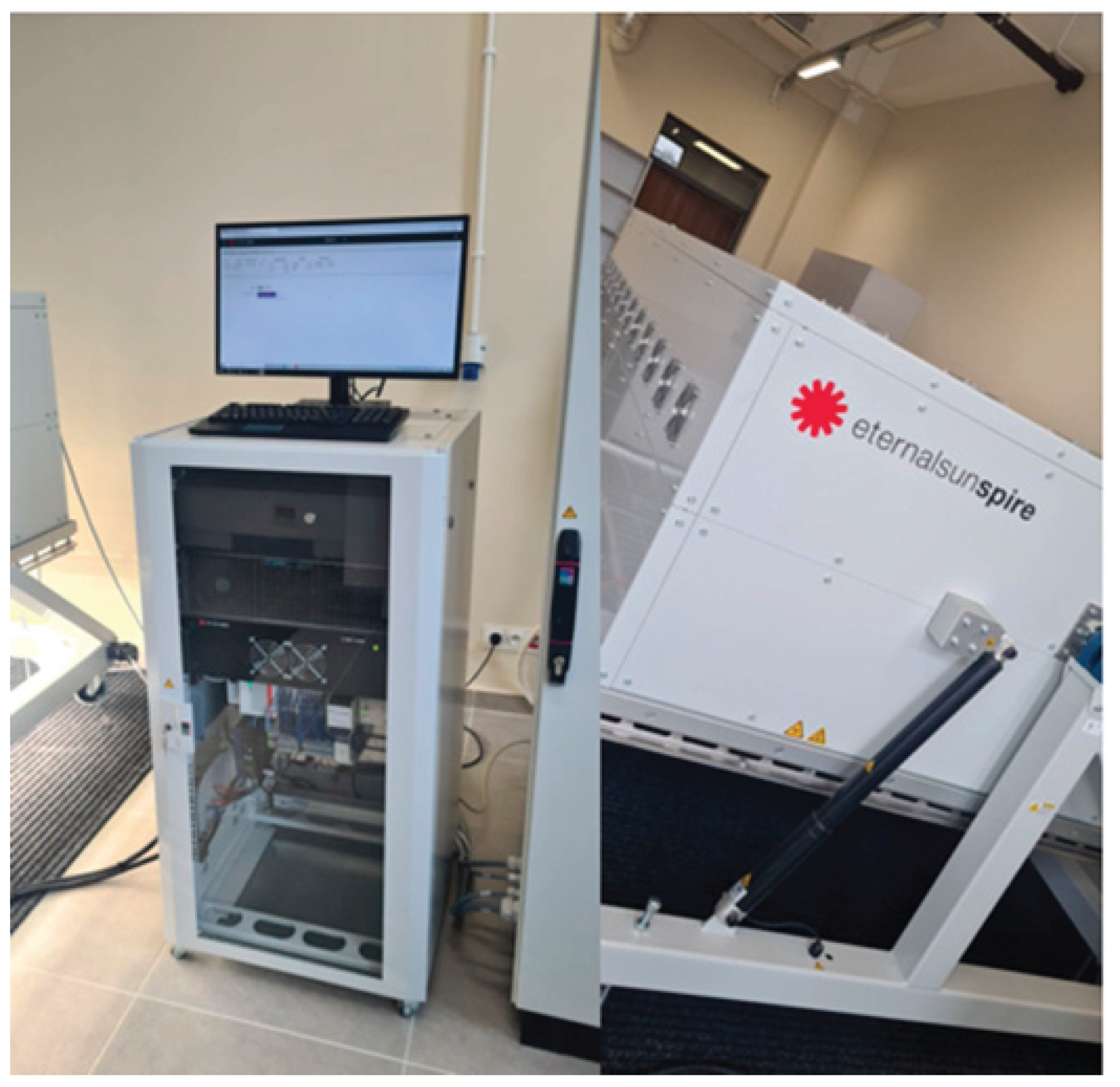
Figure 2.
View of photovoltaic modules during the test.
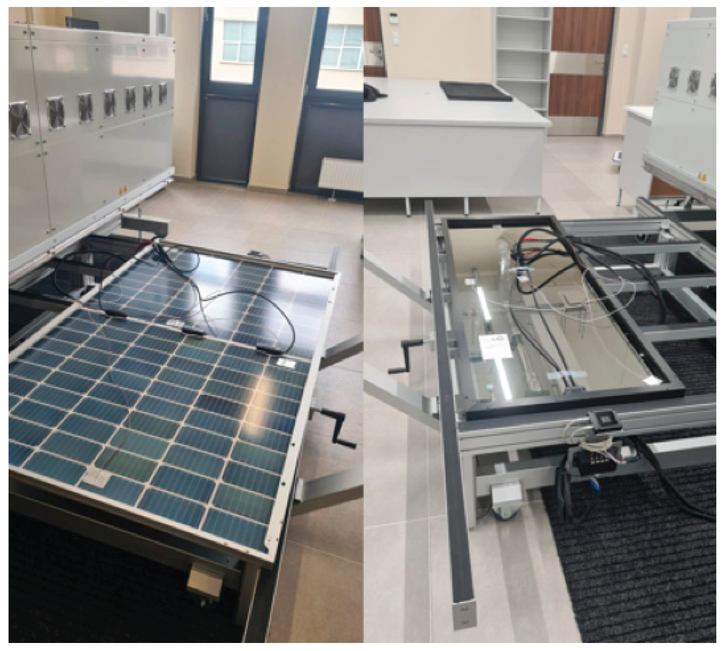
Figure 3.
Graphical representation of artificial neural network (ANN) used in this study: for every data point, the input includes features (green), the hidden layer consists of neurons (blue), and the output of the network is a vector with values and (pink).
Figure 3.
Graphical representation of artificial neural network (ANN) used in this study: for every data point, the input includes features (green), the hidden layer consists of neurons (blue), and the output of the network is a vector with values and (pink).
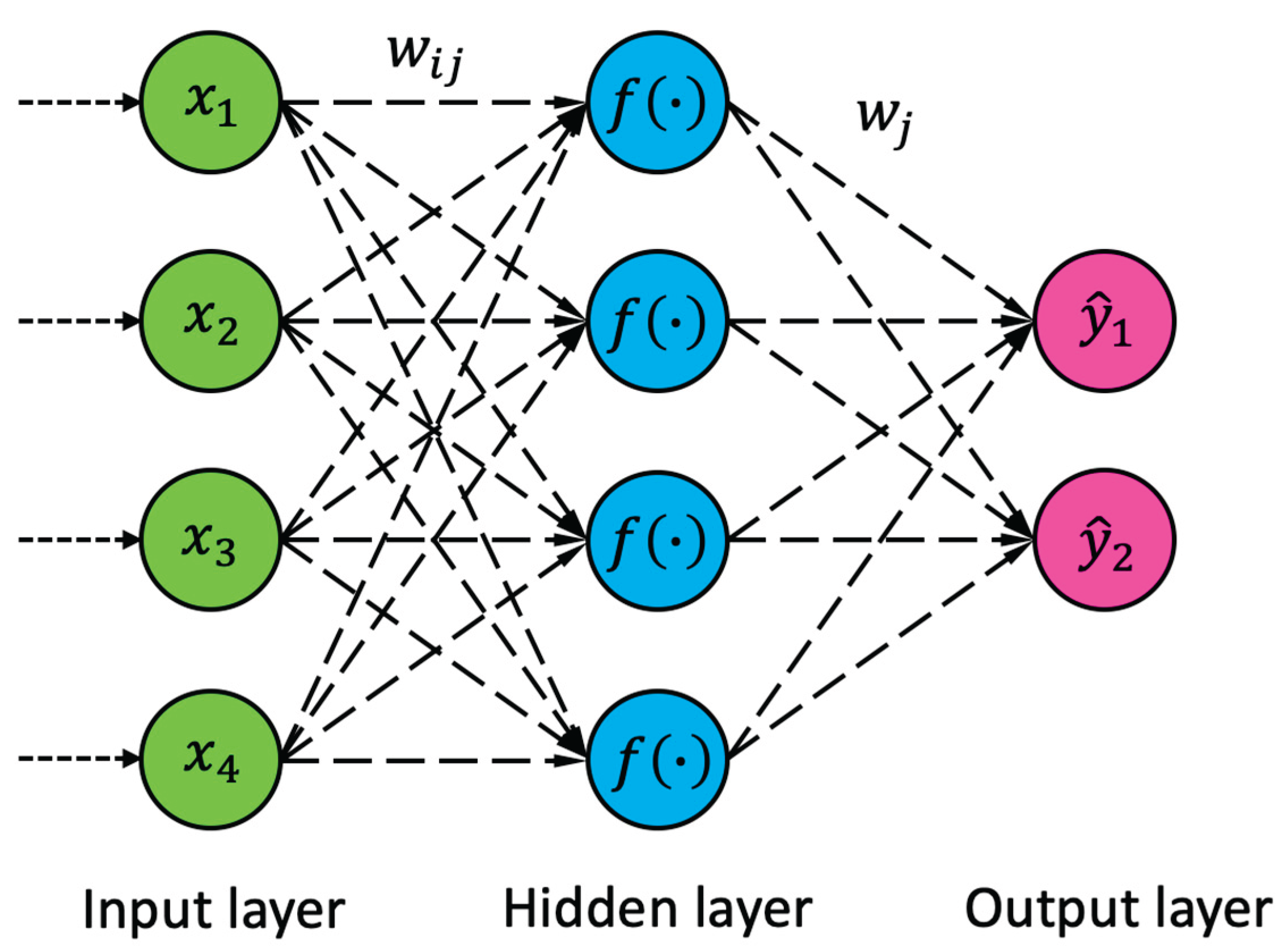
Figure 4.
Flow chart diagram for the data used and processes applied in this study.
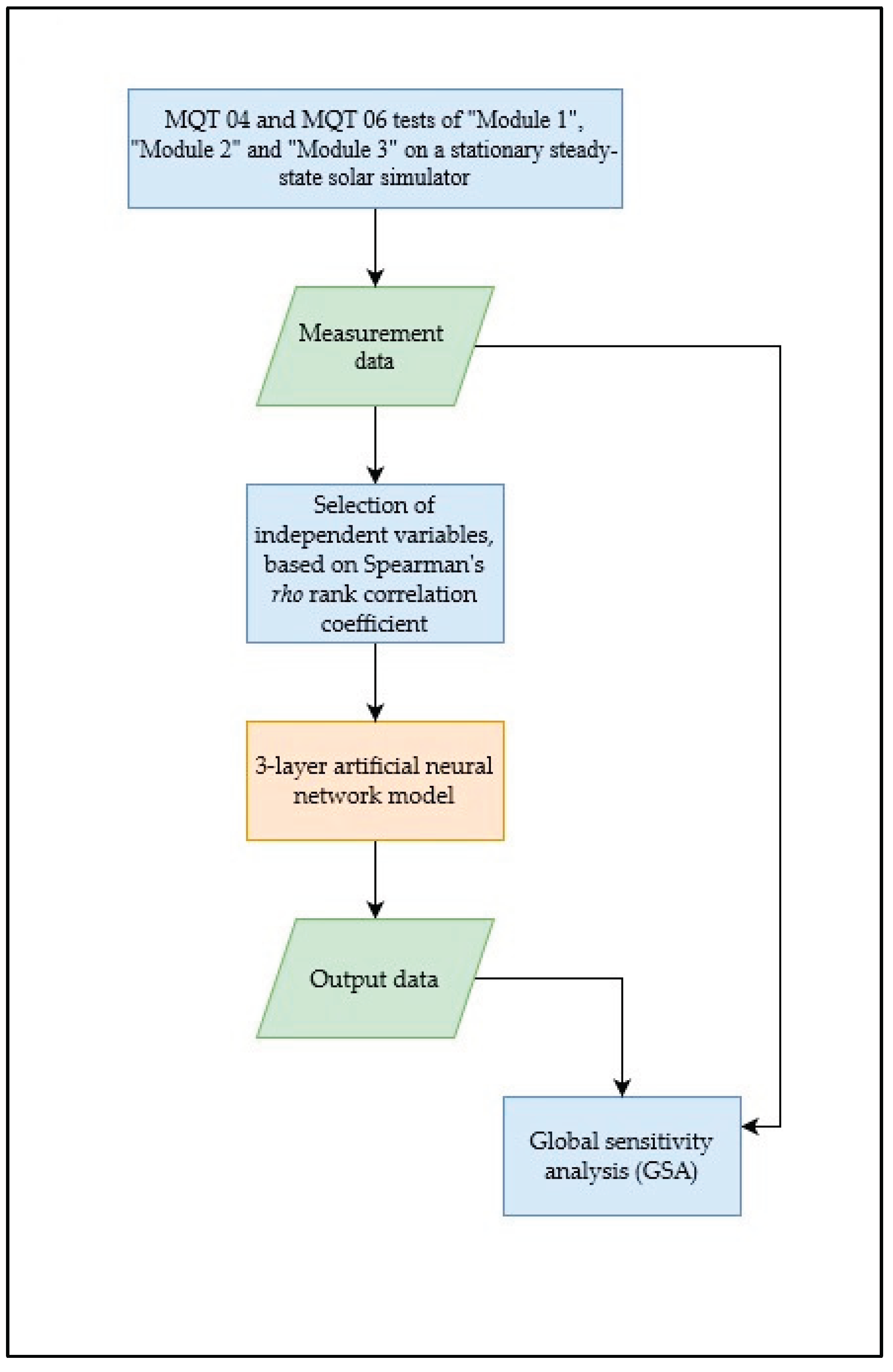
Figure 5.
Summary I-V characteristics of “Module 1”.
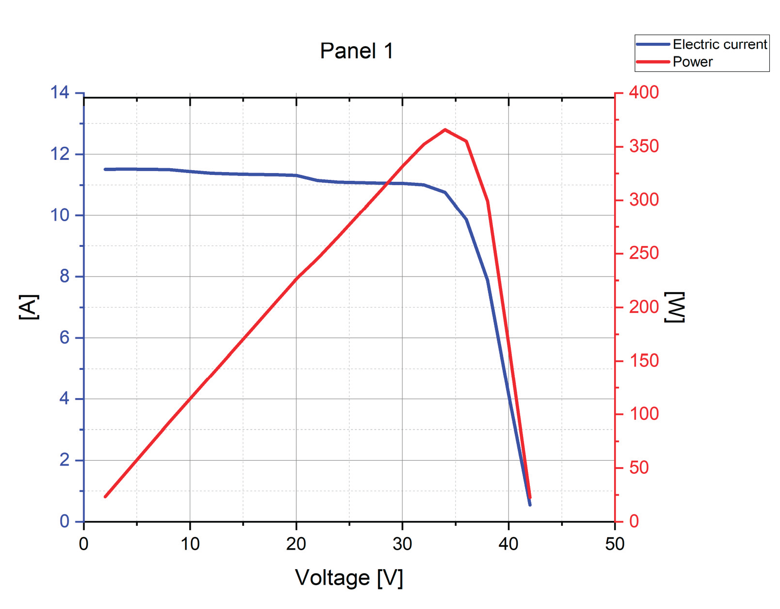
Figure 6.
Summary I-V characteristics of “Module 2”.
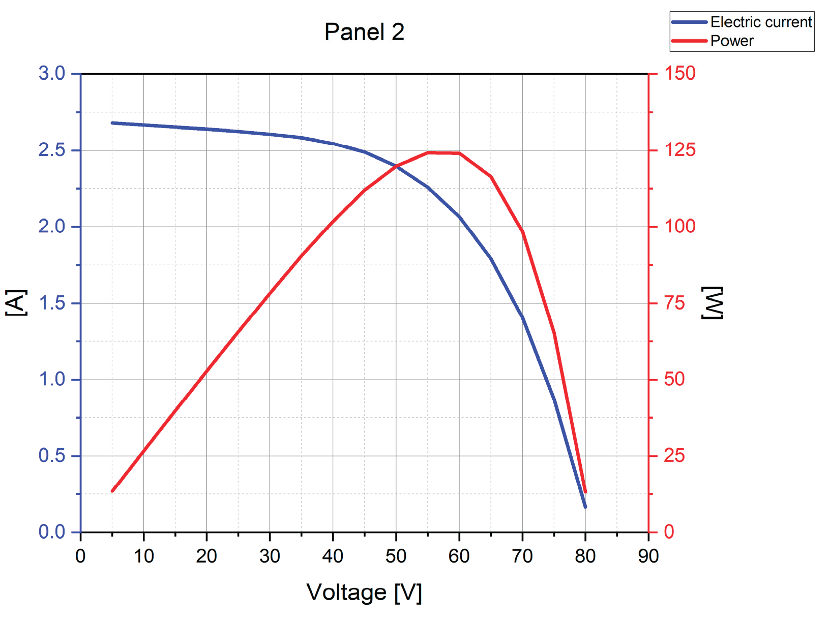
Figure 7.
Summary I-V characteristics of “Module 3”.
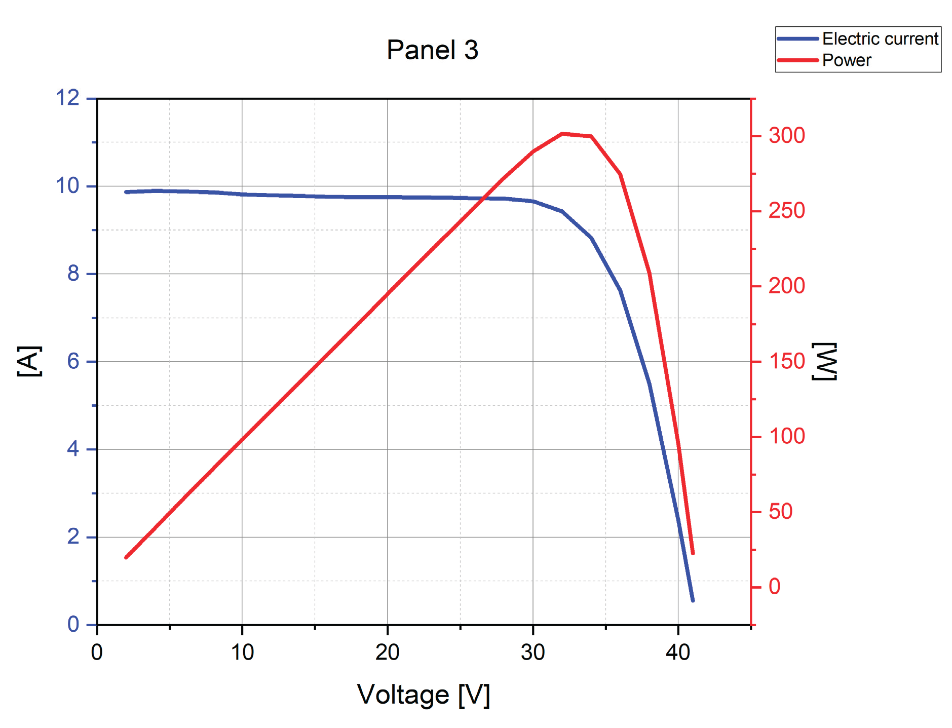
Figure 8.
Comparison of calculated with MLP model and experimentally tested characteristics of the Power [W] and the Voltage [V] for “Module 1” data.
Figure 8.
Comparison of calculated with MLP model and experimentally tested characteristics of the Power [W] and the Voltage [V] for “Module 1” data.
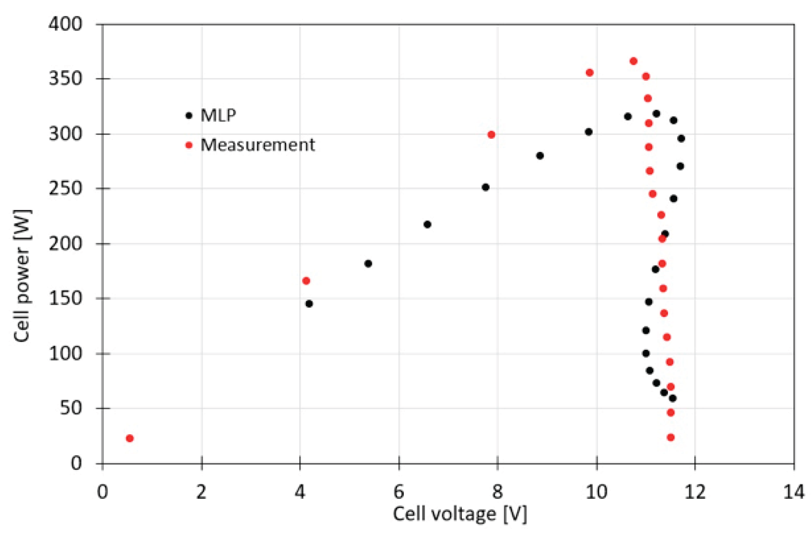
Figure 9.
Comparison of calculated with MLP model and experimentally tested characteristics of the Power [W] and the Voltage [V] for “Module 2” data.
Figure 9.
Comparison of calculated with MLP model and experimentally tested characteristics of the Power [W] and the Voltage [V] for “Module 2” data.
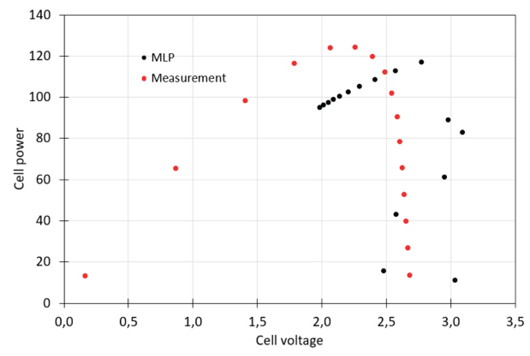
Figure 10.
Comparison of calculated with MLP model and experimentally tested characteristics of the Power [W] and the Voltage [V] for “Module 3” data.
Figure 10.
Comparison of calculated with MLP model and experimentally tested characteristics of the Power [W] and the Voltage [V] for “Module 3” data.
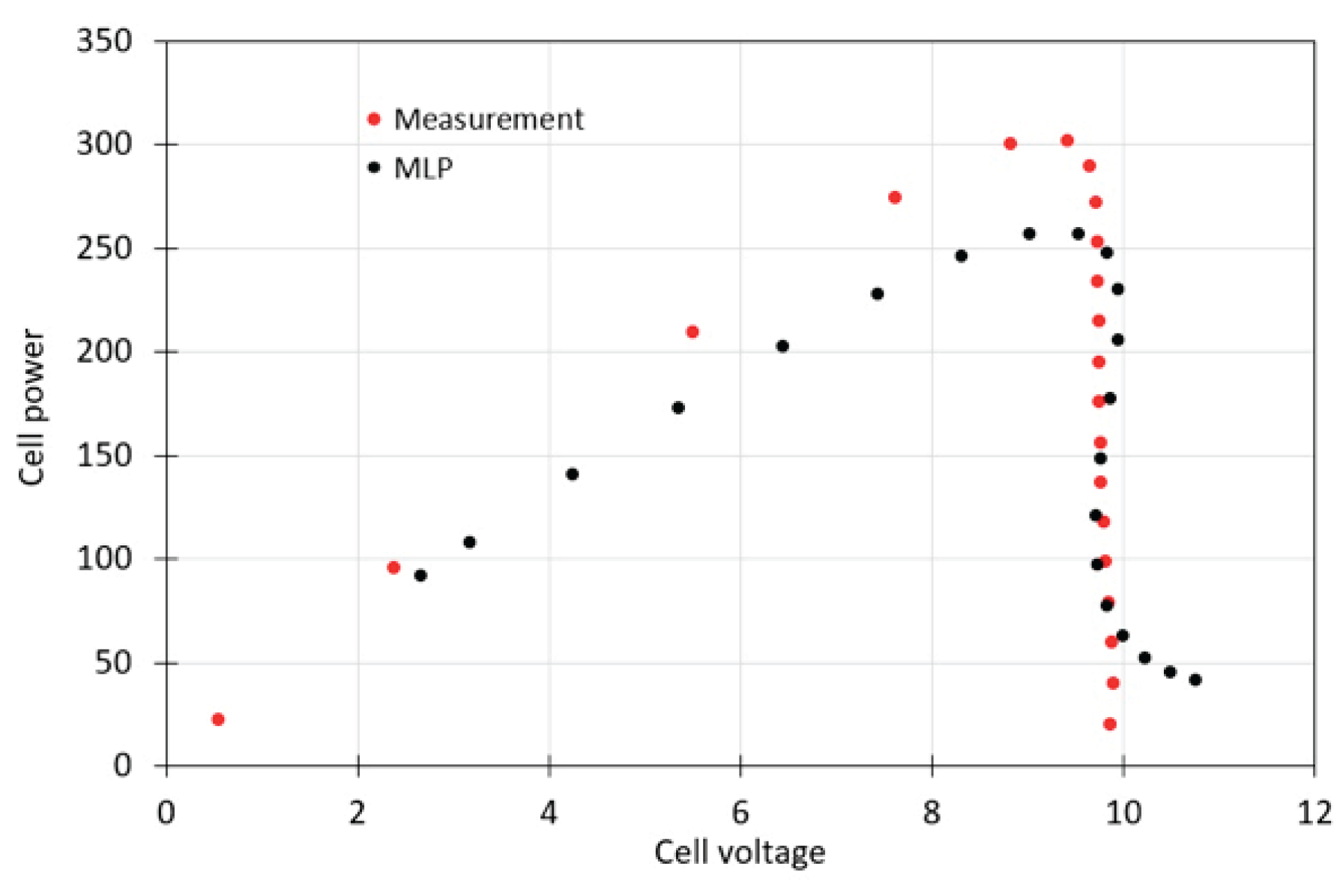

Table 1.
Characteristics of the tested photovoltaic modules.
| Parameter | PV modules tested | ||||
|---|---|---|---|---|---|
| Module 1 | Module 2 | Module 3 | |||
| Max Power | Pmax | [W] | 365 | 145 | 315 |
| Idle voltage | Voc/V | [V] | 40.7 | 59.5 | 40.53 |
| Module efficiency | Eff | [%] | 20.0 | 13.3 | 19.3 |
| Max power voltage | Vmpp | [V] | 34.1 | 60.4 | 33.2 |
| Max power current | Impp | [A] | 10.7 | 2.4 | 9.5 |
| Short-circuit current | Isc | [A] | 11.4 | 2.7 | 10.0 |
| Open-circuit voltage | Voc | [V] | 40.7 | 85.2 | 40.5 |
Table 2.
Results of module parameters obtained during measurements.
| Parameter | Module 1 | Module 2 | Module 3 |
|---|---|---|---|
| Pmax [W] | 367.302 | 125.332 | 303.844 |
| Isc [A] | 11.454 | 2.692 | 9.818 |
| Voc [V] | 44.996 | 86.334 | 49.71 |
| Impp [A] | 10.654 | 2.166 | 9.192 |
| Vmpp [V] | 34.47 | 57.804 | 32.838 |
| Filling Factor [-] | 0.712 | 0.538 | 0.622 |
Table 3.
Dependence of current and power values with averages for tested PV modules.
| Measurement | 5V | 15V | 25V | 35V | 40V |
|---|---|---|---|---|---|
| “Module 1” | |||||
| Power | |||||
| Measurement 1 [W] | 57.8901 | 171.1275 | 275.1322 | 365.42124 | 161.8382 |
| Measurement 2 [W] | 57.6934 | 170.9794 | 274.2930 | 362.1189 | 169.96 |
| Measurement 3 [W] | 57.3698 | 169.8569 | 280.7647 | 361.1334 | 168.7743 |
| Measurement 4 [W] | 57.5227 | 169.8666 | 281.0866 | 359.4855 | 161.9976 |
| Measurement 5 [W] | 57.3990 | 169.6859 | 274.4320 | 354.4239 | 165.2108 |
| Average [W] | 57.57503 | 170.3033 | 277.1417 | 360.5166 | 165.5562 |
| Current | |||||
| Measurement 1 [A] | 11.5763 | 11.409 | 11.0057 | 10.452 | 4.0459 |
| Measurement 2 [A] | 11.5389 | 11.399 | 10.9726 | 10.3584 | 4.249 |
| Measurement 3 [A] | 11.4748 | 11.325 | 11.2311 | 10.3311 | 4.2193 |
| Measurement 4 [A] | 11.507 | 11.3253 | 11.2439 | 10.2844 | 4.0499 |
| Measurement 5 [A] | 11.4799 | 11.3129 | 10.978 | 10.1403 | 4.1303 |
| Average [A] | 11.5154 | 11.3543 | 11.0863 | 10.3132 | 4.1389 |
| “Module 2” | |||||
| Power | |||||
| Measurement 1 [W] | 13.4401 | 65.8343 | 113.0481 | 119.1181 | 17.9283 |
| Measurement 2 [W] | 13.3214 | 65.1509 | 111.2806 | 114.9977 | 11.3292 |
| Measurement 3 [W] | 13.4363 | 65.8609 | 112.2522 | 116.6261 | 10.9828 |
| Measurement 4 [W] | 13.3855 | 65.2238 | 111.2941 | 115.5224 | 13.8337 |
| Measurement 5 [W] | 13.4530 | 65.9243 | 112.1763 | 115.5607 | 11.9393 |
| Average [W] | 13.4073 | 65.5988 | 112.0102 | 116.3650 | 13.2026 |
| Current | |||||
| Measurement 1 [A] | 2.6882 | 2.6334 | 2.5122 | 1.8326 | 0.2241 |
| Measurement 2 [A] | 2.6644 | 2.606 | 2.4729 | 1.7692 | 0.1416 |
| Measurement 3 [A] | 2.6873 | 2.6344 | 2.4945 | 1.7942 | 0.1373 |
| Measurement 4 [A] | 2.677 | 2.609 | 2.4732 | 1.777 | 0.1729 |
| Measurement 5 [A] | 2.6906 | 2.637 | 2.4928 | 1.7778 | 0.1492 |
| Average [A] | 2.6815 | 2.624 | 2.4891 | 1.7902 | 0.165 |
| “Module 3” | |||||
| Power | |||||
| Measurement 1 [W] | 49.4636 | 146.4109 | 243.2909 | 296.5507 | 107.8788 |
| Measurement 2 [W] | 49.5614 | 146.6602 | 243.8605 | 286.7913 | 89.9354 |
| Measurement 3 [W] | 49.5627 | 146.8454 | 243.7230 | 288.4221 | 102.8483 |
| Measurement 4 [W] | 49.4132 | 146.5157 | 242.7928 | 281.0666 | 84.2467 |
| Measurement 5 [W] | 49.2112 | 146.1223 | 242.8360 | 283.3992 | 92.6678 |
| Average [W] | 49.4424 | 146.5109 | 243.3006 | 287.2460 | 95.5154 |
| Current | |||||
| Measurement 1 [A] | 9.8910 | 9.7619 | 9.7318 | 8.4882 | 2.6970 |
| Measurement 2 [A] | 9.9170 | 9.7782 | 9.7545 | 8.2108 | 2.2484 |
| Measurement 3 [A] | 9.9121 | 9.7907 | 9.7494 | 8.2570 | 2.5712 |
| Measurement 4 [A] | 9.8839 | 9.7686 | 9.7121 | 8.0493 | 2.1062 |
| Measurement 5 [A] | 9.8459 | 9.7419 | 9.7138 | 8.1150 | 2.3167 |
| Average [A] | 9.8900 | 9.7683 | 9.7323 | 8.2241 | 2.3879 |
Table 4.
Correlation coefficients of tested PV modules.
| U | Tc | Tp | Pmax | Voc/V | eff | Vmpp | Impp | Isc | |
|---|---|---|---|---|---|---|---|---|---|
| U | 1.00 | 0.73 | 0.25 | 0.33 | 0.33 | 0.33 | 0.33 | 0.33 | 0.33 |
| Tc | 1.00 | 0.29 | 0.79 | 0.33 | 0.79 | 0.33 | 0.79 | 0.79 | |
| Tp | 1.00 | 0.44 | 0.31 | 0.44 | 0.31 | 0.44 | 0.44 | ||
| Pmax | 1.00 | 0.36 | 1.00 | 0.36 | 1.00 | 1.00 | |||
| Voc/V | 1.00 | 0.36 | 1.00 | 0.36 | 0.36 | ||||
| eff | 1.00 | 0.36 | 1.00 | 1.00 | |||||
| Vmpp | 1.00 | 0.36 | 0.36 | ||||||
| Impp | 1.00 | 1.00 | |||||||
| Isc | 1.00 |
Table 5.
Fitting measures between simulation results and measurements on dependent variables.
| Set | Tp | Tc | ||||
|---|---|---|---|---|---|---|
| Training | 0.94 | 24.68 | 36.06 | 0.97 | 0.53 | 1.17 |
| Test | 0.98 | 13.87 | 14.87 | 1.00 | 0.23 | 0.32 |
| Validation | 0.87 | 39.62 | 46.31 | 0.98 | 0.75 | 0.93 |
Disclaimer/Publisher’s Note: The statements, opinions and data contained in all publications are solely those of the individual author(s) and contributor(s) and not of MDPI and/or the editor(s). MDPI and/or the editor(s) disclaim responsibility for any injury to people or property resulting from any ideas, methods, instructions or products referred to in the content. |
© 2025 by the authors. Licensee MDPI, Basel, Switzerland. This article is an open access article distributed under the terms and conditions of the Creative Commons Attribution (CC BY) license (http://creativecommons.org/licenses/by/4.0/).
Copyright: This open access article is published under a Creative Commons CC BY 4.0 license, which permit the free download, distribution, and reuse, provided that the author and preprint are cited in any reuse.


