
Submitted:
10 June 2024
Posted:
11 June 2024
You are already at the latest version
Abstract
Photovoltaic modules should pass series of tests and examinations, verifying the electrical and thermal characteristics of the module, before being released to the market, examining the properties of the modules should undergo appropriate durability and efficiency tests under real outdoor conditions with exposure to climatic conditions and under laboratory conditions. The performance of photovoltaic cells depends on many factors, such as solar irradiance, module operating temperature, installation location, weather conditions and module shading. In this paper, three selected photovoltaic modules were examined using a large-scale steady-state solar simulator. The current-voltage (I-V) characteristics of the photovoltaic modules were experimentally tested and analyzed. The next step was to implement a three-layer artificial neural network model (MLP). The experimental data obtained in the previous step coupled with output data from MLP were then used in global sensitivity analysis (GSA). Experiments carried out on a large-scale stationary solar simulator showed differences between the values declared by the manufacturer and the values obtained from measurements of PV modules. The first module tested achieved the maximum power point greater than that specified by the manufacturer, while the other two showed power drops; it was 85-87% for the second module, and 95-98% for the third, respectively. The performed global sensitivity analysis (GSA) for the MLP model showed that the parameters: eff (22.9) and Voc/V (14.19) have the largest effect on the power-voltage relationship, while U (7.29) has the smallest effect. The usefulness of machine learning (ML) methods in the comparative analysis of PV modules has been proved.
Keywords:
photovoltaics
; current-voltage characteristics
; solar energy
; PV modules
; machine learning
; neural networks
; statistical modeling
1. Introduction and State of the Art
Electricity plays a crucial role in driving global economic and technological progress. Its ubiquitous use in daily life underscores its paramount importance. To address energy supply shortages and environmental concerns, there is a growing imperative to explore renewable energy sources as viable alternatives. This shift is driven by diminishing conventional energy resources and escalating environmental apprehensions, necessitating the exploration of alternative energy solutions to meet increasing energy demands.
One type of renewable energy source is the photovoltaics (PV) [1]. Every PV system is simple in its form and has been described as a system for generating electricity by absorbing photons from solar radiation. PV systems consist of PV modules, inverters, batteries, cables and safety devices [2]. PV modules are made of various layers, starting with the layer of glass with an anti-reflective coating, an encapsulation material, solar cell array, another encapsulation layer, and back sheet. These systems are used to handle everything from very small loads of a few watts to large power plants that can generate tens or more Megawatts of clean energy [3].
PV cell technologies are typically categorized into three generations based on the fundamental material utilized and the level of commercial maturity [3]:
- First-generation PV systems, which are fully commercialized, employ wafer-based crystalline silicon (c-Si) technology, comprising either single crystalline (sc-Si) or multicrystalline (mc-Si) structures.
- Second-generation PV systems, in the early stages of market deployment, encompass thin-film PV technologies, primarily including three main families: (1) amorphous (a-Si) and micromorph silicon (a-Si/μc-Si); (2) cadmium telluride (CdTe); and (3) copper indium selenide (CIS) and copper indium-gallium diselenide (CIGS).
- Third-generation PV systems comprise technologies such as concentrating PV (CPV) and organic PV cells, which are still in the demonstration phase or have not yet attained widespread commercialization, alongside novel concepts currently in development.
The former ones are the most widespread, well-established and reliable on the market. Crystalline silicon modules are also divided into monocrystalline (MONO-SI) or poly-crystalline (P-Si) [4]. Many researchers have described the manufacturing process and the factors that affect their efficiency. The manufacturing process uses semiconductor materials and the classification of solar cells depends on this. The aforementioned types have the same principle of converting sunlight into electricity, and the main difference is the efficiency of the conversion process itself. Basically, solar cells can have single or multiple layers or configurations that use different absorption capacities. There are also different technological generations. The first generation is based on crystalline, mono and poly-crystalline silicon, while the second and third generations are thin film and various thin film technologies [5].
The first (G1) uses crystalline silicon (c-Si) structures. Silicon is widely used because it is an abundant material on Earth and these systems show high efficiency [6]. Chapin et al. developed the first silicon solar cell in 1954 with an efficiency of 6% [7,8], and today the value is 26.1% [9]. Second-generation (G2) photovoltaic cells are based on thin-film technologies, such as CIGS solar cells. This type of photovoltaic presents lower production costs, but its efficiency is not as high as G1 [7,10,11]. In 1976, the first CIGS solar cell was developed by Kazmersky et al. with an efficiency of 4.5% [12], and in 2019, it was reported to have a maximum efficiency of 23.4% by replacing conventional CdS buffer layers with Zn double buffer layers [13]. In 2019, crystalline silicon technologies showed the cost of about EUR 0.25-EUR 0.27/W, while CIGS cost at EUR 0.48/W. Third-generation (G3) photovoltaic cells include still emerging solar technologies such as nanowire (NWs) and quantum dots (QDs) [9,14,15].
Hwang et al, [16] indicated that G3 showed efficiency around 18.9%. Solar modules have the best life-cycle of 20-30 years [17], while the life-cycle of solar inverters is less than 15 years [18] and batteries about 3-5 years [19]. Temperature is one of the parameters that can change the performance of photovoltaic modules, as can irradiate [20]. The performance of solar systems is affected by environmental conditions such as weather, climate and irradiance, while internal factors such as conductivity, uniformity of interfaces and materials can be improved by configuring the optimal characteristics of solar system [21]. Many factors can affect the performance and efficiency of photovoltaic cells, including variations in solar radiation, surface temperature, the use of shunt diodes to reduce shading losses, elimination of hotspots, orientation and tilt angle, and other additional factors.
Solar energy represents a crucial renewable solution to mitigate carbon emissions and promote environmental sustainability amid the urgency to reduce reliance on fossil fuels. Nevertheless, there are still some challenges needed to address this cutting-edge technology using artificial intelligence. As the global transition towards renewable energy sources progresses, the significance of artificial intelligence in augmenting solar energy generation rates has escalated. This technology plays a pivotal role in minimizing the wastage of renewable energy and guaranteeing a more stable electricity supply to the grid. Additionally, artificial intelligence is utilized to refine the design and positioning of solar panels, further optimizing their efficiency and effectiveness in harnessing solar energy.
Artificial intelligence has the capability to analyze various data points concerning solar panel performance, including temperature, solar radiation, and humidity levels. This is achieved by gathering data from sensors embedded within the solar panels and inputting it into machine learning models for analysis. Consequently, artificial intelligence can detect factors influencing solar panel performance, such as pollution, dust accumulation, or structural damage. It can provide valuable insights for maintenance and cleaning procedures to optimize solar energy generation. Moreover, artificial intelligence can analyze historical performance data of solar panels and forecast their future performance. Utilizing data, artificial neural networks (ANNs) for machine learning, and long short-term memory (LSTM) networks for deep learning, predictions can be made to estimate how solar panels will perform under various conditions, such as changes in solar radiation or temperature. These predictive capabilities contribute to enhancing the utilization of solar energy and improving its overall efficiency [A. A. S. Altaiy, Improving Solar Energy System Performance Using Artificial Intelligence (AI), 2024].
The landscape of solar energy forecasting has seen significant advancements due to the integration of Machine Learning (ML) and Deep Learning (DL) models. Various studies have contributed to this field, each offering unique insights and advancements. Elsaraiti et al. (2022) employed LSTM networks and MLP architectures to accurately predict solar radiation, showcasing the value of these models in improving solar energy predictions. Meanwhile, Vennila et al. (2022) presented an ensemble approach integrating multiple ML models, proving more accurate and cost-effective than individual models. Sudharshan et al. (2022) proposed hybrid and federated learning models for precise estimations of solar radiation patterns, surpassing traditional models relying on complex computations. Pombo et al. (2022) discussed challenges in obtaining consistent outcomes from ML models in Renewable Energy Systems (RES), emphasizing the importance of leveraging system features for prediction accuracy. Li et al. (2022) developed a hybrid DL model to improve the accuracy of solar energy predictions, showing potential for increased precision. Gumar et al. (2022) compared optimization algorithms for solar energy forecasts, with Particle Swarm Optimization showing the highest accuracy. Alkhayat et al. (2022) developed the ENERGY model, outperforming conventional statistical methods in accuracy for solar energy predictions. Zazoum et al. (2022) compared algorithms for predicting solar output, with GPR outperforming SVM in accuracy. Almaghrabi (2021) proposed a DL model, CLED, for forecasting solar power generation with exceptional accuracy. Zhou et al. (2021) proposed a model using IoT sensors and DL models for precise energy consumption prediction. Fara et al. (2021) evaluated ARIMA and ANN methods for solar panel output prediction, highlighting their strengths and weaknesses. Konstantinou et al. (2021) explored stacked LSTM models for predicting solar power generation, optimizing hyperparameters for best performance. Alkhayat (2021) provided a comprehensive study on DL models and techniques, evaluating their effectiveness and current research status. Shamshirband et al. (2019) applied DL methods to enhance solar energy forecast accuracy, with RNN and LSTM models performing well. Abdelhakim et al. (2016) discussed integrating EMS with forecasting techniques for efficient clean energy generation. Alamin et al. (2020) created an ANN model for forecasting energy output in HCPV systems, capturing CPV system performance accurately. Mellit et al. (2020) examined AI methods for predicting solar power generation, emphasizing the need for quality datasets and considering external factors. Zhang et al. (2018) proposed an ensemble method for solar power prediction, outperforming other models. Overall, these studies highlight the rapid advancements in solar power forecasting methodologies, particularly leveraging ML and DL techniques to provide accurate predictions and address existing shortcomings [55-73].
Photovoltaics also raise many questions and unknowns to scientists, researchers and engineers around the globe. One challenge is the increase in surface temperature, especially in countries with high solar radiation. Nabil and Mansour [22] studied the performance of polycrystalline silicon (PV) photovoltaic modules using different cooling systems and compared the performance of PV modules with and without cooling. For each degree of temperature increase, the maximum output power of the PV modules tested decreases by up to 0.42%. The surface temperature of the solar panels increases when they are exposed to direct sunlight, resulting in a significant decrease in the electrical output power of the PV cells. The lifespan of PV modules can be extended by proper cooling, as it increases the electrical output while slowing the rate of cell degradation [23]. Kumar [24] conducted experiments to study how the surface temperature of a PV module can affect its electrical characteristics. The researchers found that for a 5 W PV module, each 1°C increase in PV module surface temperature resulted in a 0.4% decrease in open circuit voltage. Similarly, for every 1°C increase in module surface temperature, there was a 0.6% and 0.32% decrease in maximum power, respectively. In contrast, the short-circuit current increases at a rate of 0.09% per °C as the surface temperature increases. Transparent acrylic sheets began to be mounted in silicon modules, which reduced the temperature of the photovoltaic surface, thereby improving efficiency, increasing electricity production and extending the life of the cells. They mounted 3 mm acrylic sheets parallel to the photo-voltaic panel and 30 cm from the top, this reduced the surface temperature by 10% compared to photovoltaics without acrylic. The largest percentage decrease in temperature, or 14.5% on the surface of the modules, was achieved by mounting the acrylic sheet at 30° angle to the module [25].
Cooling PV systems continues to be a challenge for researchers. Du et al [26] analyzed a cooling system using the active cooling system pump. It works by taking heat away from the PV and dissipating it using a convector or heat sink. Several researchers stressed that active cooling is more efficient and suitable for high concentrations. The researchers, in an experiment conducted, reported that the efficiency of solar cell with concentration is 4.7 to 5.2 times higher than a cell without concentration. The results show that the temperature of the solar cell was lowered to below 60°C, generating more electrical power. Mallick et al. performed some study using parabolic concentrators to analyze heat transfer in photovoltaics [27]. The researchers found that the temperature of the concentrator and PV cell increased with the intensity of incident solar energy. The cooling system ensures that the cell operates at the optimal temperature. CPV cooling design typically has thermal resistance factors with good cell temperature uniformity for maximum efficiency [28].
Other common problems with PV systems include hail, dust and surface operating temperatures, which can degrade conversion system performance. Environmental elements that affect PV module surface temperatures include wind speed, ambient temperature, relative humidity, accumulated dust and solar radiation. Each 1°C increase in PV module surface temperature results in a 0.5% decrease in efficiency [29].
Hoque et al. designed a PV panel cooling system using a rectangular hollow fin, a DC fan and a water atomizer on one side. The results showed that the efficiency of the solar PV panel system was increased from 17% without the cooling system to 22% with the cooling system. The temperature of the solar panel during the test period was 24°C lower than its normal operating temperature [30].
Solar simulators provide predictable and repeatable solar radiation, and have become indispensable tools for the efficient development of PV modules. For solar radiation prediction, many predictive data mining methods are successfully used, where, artificial neural networks (ANN) can be easily and widely used [31]. Many researchers have studied the implementation of ANN as a tool for predicting the performance of PV and PV/T systems. These methods are classified as experimental mathematical models, regression, network-based artificial intelligence, and finally statistical models based on a time series of data [32,33]. In general, the other, simpler ML methods, for example decision trees indeed have their advantage of requiring relatively little amount of data and in fact, they could be applied instead of ANNs. However, a single regression or classification tree tends to be “unstable”, which means that its output can differ strongly even under the influence of slight changes in the training data. At the same time ANNs are considered as more “flexible” algorithm with the possibility of free defining their structure, dedicated for multitude of various tasks falling under regression, classification or even data augmentation (e.g. GANs).
Electricity serves as a cornerstone for global economic and technological advancement, permeating various facets of daily life with indispensable utility. In response to the pressing challenges of energy supply deficits and environmental degradation, the exploration of renewable energy sources has gained momentum as a viable solution. This imperative stems from dwindling conventional energy resources and escalating environmental concerns, compelling a paradigm shift towards sustainable energy alternatives to meet burgeoning energy demands.
The specific work makes notable contributions to this discourse by conducting a comprehensive analysis of the efficiency and feasibility of integrating renewable energy sources into existing energy infrastructures, offering novel insights into the socio-economic implications and policy frameworks necessary for fostering renewable energy adoption, and proposing innovative strategies for optimizing renewable energy utilization to mitigate environmental impact while concurrently supporting economic growth. Through these contributions, this work seeks to advance our understanding and implementation of renewable energy solutions in addressing the global energy challenge.
2. Materials and Methods
2.1. Testing Methods for PV Modules
The dynamic development of the photovoltaic industry after 2000 has necessitated the creation of a set of standards and regulations, which will enable a consistent certification process for photovoltaic modules. In EU countries, certification is carried out in accordance with the standards of the International Electrotechnical Commission (IEC). IEC 61215 [34] establishes requirements for construction qualification and type approval for photovoltaic modules for terrestrial applications suitable for long-term operation under typical climatic conditions as defined in IEC 60721-2-1 [35]. The tests specified in the standard determine the performance of photovoltaic modules under the test. The standard applies to all modules made of crystalline silicon, as well as to thin-film modules. The test methodologies that were performed within the scope of this work, can be defined as the following:
- MQT 04 - Measurement of temperature coefficients - The test consists of measuring the temperature coefficients of current, voltage and peak power in accordance with PN-EN 60904-10. The purpose of the test is to determine the temperature coefficients of PV modules at different irradiances. When performing the test, a device for controlling the temperature of the module is required [34].
- MQT 06 - Performance under STC and NOCT conditions - The test consists of determining the electrical performance of the module under standard test conditions. Measurement under STC (Standard Test Conditions) is used to verify the information on the module's nameplate. The solar source should be a natural solar source or a BBA-class solar simulator, or better [34].
2.2. Characteristics of the Tested PV Modules
The first module tested is the monocrystalline, double-sided module (Figure 1a), titled “Module 1”. The module's efficiency according to the manufacturer's materials is 20%, and the maximum power is 365 Watts. The manufacturer provides 30-year warranty for the additional linear power output, which should be about 85% after 30 years [36].
The second module tested is the CIGS thin-film module (Figure 1b), titled “Module 2”. The efficiency of the module is about 13%, and the maximum power the module can produce is 145 W. The panel is double-glazed, which prevents micro-cracking and increases the module's durability. The developer guarantees a minimum power rating of 80% after 25 years [37].
The third module is the monocrystalline single-side photovoltaic module (Figure 1c), titled “Module 3”, with an efficiency of about 19.3%, and the power the module can produce is 315 watts. The developer guarantees to keep the module's degradation constant for 25 years [38]. The Table 1 shows the characteristics of the tested modules.
2.3. Experimental Description and Test Methods
The research was conducted on a stationary steady-state solar simulator, Class AAA (Figure 2), used to measure the performance of photovoltaic modules under controlled parameters. The device accurately simulates solar radiation under specified test conditions to measure the maximum output power of each tested photovoltaic module under standard test conditions. Each of the tests were done 5 times for every module and based on that we approximated results. All tested PV modules were brand-new, which means never used before (Figure 3).
The measurement device includes a large-area stationary steady-state solar simulator and photovoltaic module current-voltage analysis system as well as the calibrated accredited reference coil. The reference coil was placed on tested module, and it was used to read the reference measurements and compare them with those of the module under the test [39].
The MQT 06 and MQT 04 tests were carried out on a stationary large-scale steady state solar simulator. Conducting the MQT 06 test, it involves measuring the electrical parameters of the module under STC conditions. That means the solar irradiance of (1000±100) W/m2, and ambient temperature of the cells during the test of (25±2)°C. The connected module placed on experimental set-up with a reference coil is slid under the calibrated simulator lamps, then the measurement was started.
In the case of MQT 04, we made 10 measurements per every PV module, 5 measurements with the result correction to 25°C, 5 measurements without such correction. Before each measurement, the PV module temperature was measured before and after the test.
An important step in this paper was the construction of machine learning (ML) models to assess and select the correlation of independent variables for numerical simulations based on experimental results. The values of the correlation coefficient () range from to . Positive magnitudes of () coefficient indicate that an increase in the independent variable leads to an increase in , while negative values indicate an inverse relationship. In our ML model we used the Spearman's rho rank correlation coefficient [40], which is dedicated to the analysis of processes that are nonlinear in nature.
In our machine learning prediction model (MLP), the input signals () arriving at the input layer were multiplied by the values of the weights (), according to the Figure 4. The resulting sums went through the transformation using linear or nonlinear activation function (exponential function, hyperbolic tangent, sine, logistic function) and then were passed to the neurons (or neuron) of the output layer. The estimation of the value weight () in ANN model was carried out at the learning stage using appropriate numerical algorithms [41] to minimize the mean squared error (MSE):
where is the ground truth for the -th training data point, is the corresponding output from the neural network, , and is the number of data points in the training set.
Each coordinate of the output was calculated according to the following formula:
where: - the number of inputs to the model, - the number of neurons in the hidden layer, - the values of weights between the inputs and the neurons of the hidden layer, – neuron loads of the hidden layer, - the values of weights between neurons of the hidden layer and neuron of the output layer, - the activation function. At the stage of creating the MLP model, it is crucial to determine the number of neurons in the hidden layer. According to general recommendations, the number of neurons () in the hidden layer should be no less than the number of explanatory variables (), but no more than [42]. To avoid overfitting of the model, Rogers and Dowl [43] suggested that the value of should not be less than (where is the number of data observations in the learning set). The number of neurons in the hidden layer can also be determined by trial and error method minimizing the prediction error, but not allowing overlearning of the model (when with an increase in the prediction error increases, there is a decrease in the generalization ability of the model). This paper adopts the 3-layer neural network model with inputs including current-voltage characteristics of the PV module. For the input data, two outputs are defined, i.e. power-voltage characteristics of PV module. To build the model, 3 sets of learning (70%), test (15%), validation (15%) were adopted. At the same time, the global sensitivity analysis was performed to identify the parameters that have the key impact on the power-voltage characteristics. For this purpose, the sensitivity coefficients were determined as well.
The following measures were used to assess the correspondence between the ground truth of any of the measurement coordinates for the -th validation data point and the corresponding predicted output from the neural network:
- a)
- Coefficient of determinacy ():
- b)
- Mean absolute error (MAE):
- c)
- Root mean square error (RMSE):
3. Results
Five measurements were taken for each of the three modules, the values were averaged and approximated, as it is shown in Table 2.
The maximum power point during the test under STC conditions for “Module 1” was the highest during the 1st measurement (Figure 6). It reached 372 W, which is 102% of the manufacturer's stated maximum power of 365 W. In only one case there was the maximum power during the test less than the module manufacturer's declaration. The Filling Factor averaged value was around 0.7.
The maximum power point during the test for “Module 2” was the highest during the 1st measurement (Figure 7). It was 127W, which is only 87% of the manufacturer's stated maximum power of 145W. During the second measurement, the maximum power point was the lowest of all five measurements, at 124W, 85% of the manufacturer's stated maximum power. The Filling Factor averaged value was around 0.54, which is very low. Tested “Module 2” was the CIGS thin-film module and its efficiency was significantly lower than the first-generation module tested.
The maximum power point during the last test for “Module 3” was the highest during the 1st measurement (Figure 8). It was about 309 W, which is 98% of the manufacturer's stated maximum power of 315 W. In no case the maximum power exceeded the maximum power listed on the module manufacturer's declaration. The Filling Factor averaged value was around 0.62. Table 3 shows the difference in current versus voltage with the approximation.
Table 4 shows the correlation coefficients for each parameters of every tested PV module. Our calculations showed that the best predictive abilities were characterized by the MLP model (4:4:2) for the activation function in the hidden layer of hyperbolic tangent and linear output. The values of fitting measures between simulation results and measurements are given in Table 5. The model achieved the worst classification quality on the validation set for the variable Tp. The variable Tc was predicted by the MLP with smaller error on each of the three sets. The error was very small, as the MAE did not exceed 0.75 on each of the datasets.
4. Discussion
Comparing the approximations of the three modules, one can see the significant differences between them. The approximation of “Module 2” has a significantly higher na-voltage to lower current range compared to the approximations of “Module 2” and “Module 3”. This may be due to the chemical composition of the second module structure. The module is a CIGS thin-film, made from a combination of copper, indium, gallium and selenium. “Module 1” and “Module 3” are monocrystalline modules. Their approximations are not significantly different from each other, the voltage ranges of the modules are almost identical, the most distinctive are the cell power range and the maximum power point.
Moreover, the results of the global sensitivity analysis (GSA) for the model showed that eff (22.9) and Voc/V (14.19) have the largest effect on the power-voltage relationship, and U (7.29) has the smallest effect. Figure 9, Figure 10 and Figure 11 show the comparison of calculated power-voltage curves for Modules 1, 2 and 3. Clouds of points calculated with MLP arrange themselves into similar curves to those that were measured, however, the worst shape of the three modules’ curves has the one obtained in “Module 2”. Coefficient R2 values show a very good performance of applied neural network.
Testing of photovoltaic modules is important not only for manufacturers of photo-voltaic modules, but also for investors and system users. All photovoltaic modules should pass series of tests and examinations verifying the electrical and thermal characteristics of the module before being certified and released to the global market. To study the I-V characteristics of PV modules, they are subjected to appropriate durability and efficiency tests under real outdoor conditions with exposure to ambient conditions and under laboratory conditions. The standardization of testing methodologies for photovoltaic modules come-up from different manufacturers, is intended to standardize the products by carrying out the recommendations contained in the standards. The performance of photovoltaic cells depends on many factors, such as solar irradiance, module operating temperature, installation location, weather conditions and module shading. This causes some important differences in the performance of the modules, and differentiates them from the parameters stated in the certifications of manufacturers of photovoltaic products. Using certified products, however, guarantees that the parameters of the modules are consistent with the manufacturer's declarations in the module data sheet or on its nameplate. Thus, the original comparative analysis of different PV modules, in terms of their I-V characteristics and other parameters, as shown in this paper, is crucial for the assessment of efficiency of devices powered by renewable energy.
Various types of neural networks have been used in the past for applications related to environmental engineering. In works [44,45] neural network were applied for evaluation of soil pollution and potatoes quality changes during storage, whereas in papers [46,47] authors analyzed wastewater quality and identified activated sludge bulking. Artificial neural networks were also utilized in applications related to PV modules. In the paper [48], a neural network with two hidden layers (10:7:5:3) was used to predict the power output of PV modules based on 2 years of historical data. The neural network model was compared with a symbolic regression model and hybrid model, in which both methods mentioned above were used. The neural network performed worse than the hybrid model, but it achieved a coefficient of determination of 0.99. Whereas in [49] a Radial Basis Function (RBF) network was also applied for prediction of power output. Authors trained 3 different neural network models for sunny, cloudy and rainy weather. Best results were obtained for sunny weather, where the correlation coefficient amounted between 96% and 99%, in contrast the coefficient for rainy weather was only between 49% and 81%. In the article [50] authors used a 3:11:17:24 MLP network to predict solar irradiance in the city of Trieste, Italy. This factor is particularly important for planning power dispatching for Grid Connected Photovoltaic Plants. The correlation coefficient between data calculated by the model and measured on sunny days was 98-99%, while it was 94-96% on cloudy days. On the other hand, the coefficient of determination, for the data resulting from the model was 0.9. In work [51] Recurrent Back Propagation Network (RBPN) was also applied for solar irradiance prediction. In this paper the RMSE was equal to 3.6511 on the training and 3.8298 on the test set. Improving this result was achieved by using wavelet analysis on the results of the neural network. In paper [52] researchers showed a method of generating hourly irradiation data by using MLP models. In [53] authors used Multilayered Feedforward Neural Network for forecasting hourly total radiation valued and compared it to the results obtained by applying autoregressive model. The neural network approach was found to predict data more accurately than the AR model. In paper [54] authors compared results of several types of neural networks for prediction of mean hourly solar radiation. The best predictions were obtained by Levenberg Marquardt multivariate feed-forward neural network, where the RMSE amounted 27.58. Work [55] presents hybrid approach to artificial neural networks for forecasting global solar radiation. Authors applied MLP-MTM model, which is multilayer perceptron with Markov transition matrices. The maximum RMSE resulting from this model was 8%. As it can be concluded, most of the previous works regarding the use of neural networks in analyzing PV systems has been focused on prediction or forecasting various parameters. In comparison, this work showed that the application of a very simple 3-layer ANN (4:4:2) can also provide reliable information about the differences in various PV panels’ performance. The usefulness of machine learning algorithms in the comparative analysis of PV modules has been proved. Moreover, the global sensitivity analysis (GSA) for the performed model showed that the parameters: eff (22.9) and Voc/V (14.19) have the largest effect on the power-voltage relationship, while U (7.29) has the smallest effect.
One should bear in mind that the research presented in this work has also its limitations. The possibility of free defining the structure of ANNs can, in some cases, be an obstacle, rather than a benefit. Seeking of the optimal networks architecture is often achieved through trial & error method. It is possible to apply some other ML algorithms (e.g. tree-based models, support vector machine) and compare their results. It also could be a good future direction for this study.
5. Conclusions
Tests carried out on a large-scale stationary solar simulator showed differences between the photovoltaic module, including declared manufacturer's values and the values obtained during measurements. In case of “Module 1”, the differences between the measurements were negligible, and often the module's maximum power point during the measurement came out higher than that specified by the manufacturer. However, the results developed when testing on “Module 2” and “Module 3” showed power drops. The measured power for “Module 3” ranged from 95-98% of the manufacturer's stated power, which is not a significant result, but for “Module 2” these differences were greater, the measured power for “Module 2” was 85-87% of the module manufacturer's declared power. The manufacturer of “Module 2” in the data sheet noted the possibility of a disparity between the electrical parameters stated in the module's technical materials and those measured in use by 10%, while the differences for this module were much more than the 10% assumed by the manufacturer. The reported power drops may have been caused by the storage of the modules or their infrequent operation due to their use for research purposes. The modules were brand-new before the tests, which means never used in any circumstances.
Author Contributions
For research articles with several authors, a short paragraph specifying their individual contributions must be provided. The following statements should be used “Conceptualization, R.P. and B.S.; methodology, D.K., R.P., M.S-M.; A.L. software, B.S., A.B..; investigation, R.P., D.K., T.G., B.S.; writing—original draft preparation, R.K.,T.G., E.S.; writing, review and editing, E.Ł., M.P-R.. All authors have read and agreed to the published version of the manuscript.
Funding
Research project supported by the program "Excellence Initiative – Research University" for the AGH University of Krakow as well as the subvention funding source from the Ministry of Science and Higher Education of Poland dedicated for Lublin University of Technology.
Acknowledgments
Authors would like to thank the whole team of Eternasun Spire and ANKO (Andrzej Kołaczkowski) for the preparation and delivery of solar steady-state simulator as well as Elias Garcia Goma from Solar Chills for his perfect guidance on I-V characteristics and measurements.
Conflicts of Interest
The authors declare no conflict of interest.
References
- Maka, A.O.M.; Alabid, J.M. Solar Energy Technology and Its Roles in Sustainable Development. Clean Energy 2022, 6, 476–483. [Google Scholar] [CrossRef]
- Aktaş, A.; Kirçiçek, Y. Solar System Characteristics, Advantages, and Disadvantages. In Solar Hybrid Systems; Elsevier, 2021; pp. 1–24.
- Winter, A.; Hager, M.D.; Newkome, G.R.; Schubert, U.S. The Marriage of Terpyridines and Inorganic Nanoparticles: Synthetic Aspects, Characterization Techniques, and Potential Applications. Adv. Mater. 2011, 23, 5728–5748. [Google Scholar] [CrossRef] [PubMed]
- Bdour, M.; Al-Sadi, A. Analysis of Different Microcracks Shapes and the Effect of Each Shape on Performance of PV Modules. IOP Conf. Ser. Mater. Sci. Eng. 2020, 876, 012005. [Google Scholar] [CrossRef]
- Mohammad Bagher, A. Types of Solar Cells and Application. Am. J. Opt. Photonics 2015, 3, 94. [Google Scholar] [CrossRef]
- Green, M.A. Silicon Photovoltaic Modules: A Brief History of the First 50 Years. Prog. Photovoltaics Res. Appl. 2005, 13, 447–455. [Google Scholar] [CrossRef]
- El Chaar, L.; Lamont, L.A.; El Zein, N. Review of Photovoltaic Technologies. Renew. Sustain. Energy Rev. 2011, 15, 2165–2175. [Google Scholar] [CrossRef]
- Goetzberger, A.; Hebling, C.; Schock, H.-W. Photovoltaic Materials, History, Status and Outlook. Mater. Sci. Eng. R Reports 2003, 40, 1–46. [Google Scholar] [CrossRef]
- Marques Lameirinhas, R.A.; Torres, J.P.N.; de Melo Cunha, J.P. A Photovoltaic Technology Review: History, Fundamentals and Applications. Energies 2022, 15, 1823. [Google Scholar] [CrossRef]
- Asdrubali, F.; Umberto, D. High Efficiency Plants and Building Integrated Renewable Energy Systems. In Handbook of Energy Efficiency in Buildings; Elsevier, 2019; pp. 441–595.
- Sahu, A.; Garg, A.; Dixit, A. A Review on Quantum Dot Sensitized Solar Cells: Past, Present and Future towards Carrier Multiplication with a Possibility for Higher Efficiency. Sol. Energy 2020, 203, 210–239. [Google Scholar] [CrossRef]
- Lee, T.D.; Ebong, A.U. A Review of Thin Film Solar Cell Technologies and Challenges. Renew. Sustain. Energy Rev. 2017, 70, 1286–1297. [Google Scholar] [CrossRef]
- Nakamura, M.; Yamaguchi, K.; Kimoto, Y.; Yasaki, Y.; Kato, T.; Sugimoto, H. Cd-Free Cu(In,Ga)(Se,S) 2 Thin-Film Solar Cell With Record Efficiency of 23.35%. IEEE J. Photovoltaics 2019, 9, 1863–1867. [Google Scholar] [CrossRef]
- Sinke, W.C. Development of Photovoltaic Technologies for Global Impact. Renew. Energy 2019, 138, 911–914. [Google Scholar] [CrossRef]
- Pinho Correia Valério Bernardo, C.; Marques Lameirinhas, R.A.; Neto Torres, J.P.; Baptista, A. Comparative Analysis between Traditional and Emerging Technologies: Economic and Viability Evaluation in a Real Case Scenario. Mater. Renew. Sustain. Energy 2023, 12, 1–22. [Google Scholar] [CrossRef]
- Hwang, I.; Um, H.-D.; Kim, B.-S.; Wober, M.; Seo, K. Flexible Crystalline Silicon Radial Junction Photovoltaics with Vertically Aligned Tapered Microwires. Energy Environ. Sci. 2018, 11, 641–647. [Google Scholar] [CrossRef]
- Weckend, S.; Wade, A.; Heath, G. End of Life Management: Solar Photovoltaic Panels; Golden, CO (United States), 2016.
- Sangwongwanich, A.; Yang, Y.; Sera, D.; Blaabjerg, F. Lifetime Evaluation of Grid-Connected PV Inverters Considering Panel Degradation Rates and Installation Sites. IEEE Trans. Power Electron. 2018, 33, 1225–1236. [Google Scholar] [CrossRef]
- Manimekalai, P.; Harikumar, R.; Raghavan, S. An Overview of Batteries for Photovoltaic (PV) Systems. Int. J. Comput. Appl. 2013, 82, 28–32. [Google Scholar] [CrossRef]
- Pinho Correia Valério Bernardo, C.; Marques Lameirinhas, R.A.; Neto Torres, J.P.; Baptista, A. The Shading Influence on the Economic Viability of a Real Photovoltaic System Project. Energies 2023, 16, 2672. [Google Scholar] [CrossRef]
- Karthikeyan, V.; Sirisamphanwong, C.; Sukchai, S.; Sahoo, S.K.; Wongwuttanasatian, T. Reducing PV Module Temperature with Radiation Based PV Module Incorporating Composite Phase Change Material. J. Energy Storage 2020, 29, 101346. [Google Scholar] [CrossRef]
- Nabil, T.; Mansour, T.M. Augmenting the Performance of Photovoltaic Panel by Decreasing Its Temperature Using Various Cooling Techniques. Results Eng. 2022, 15, 100564. [Google Scholar] [CrossRef]
- Gupta, V.; Sharma, M.; Pachauri, R.K.; Dinesh Babu, K.N. Comprehensive Review on Effect of Dust on Solar Photovoltaic System and Mitigation Techniques. Sol. Energy 2019, 191, 596–622. [Google Scholar] [CrossRef]
- Agyekum, E.B.; PraveenKumar, S.; Alwan, N.T.; Velkin, V.I.; Shcheklein, S.E. Effect of Dual Surface Cooling of Solar Photovoltaic Panel on the Efficiency of the Module: Experimental Investigation. Heliyon 2021, 7, e07920. [Google Scholar] [CrossRef] [PubMed]
- Murtadha, T.K. Installing Clear Acrylic Sheet to Reduce Unwanted Sunlight Waves That Photovoltaic Panels Receive. Results Eng. 2023, 17, 100875. [Google Scholar] [CrossRef]
- Du, B.; Hu, E.; Kolhe, M. Performance Analysis of Water Cooled Concentrated Photovoltaic (CPV) System. Renew. Sustain. Energy Rev. 2012, 16, 6732–6736. [Google Scholar] [CrossRef]
- Mallick, T.K.; Eames, P.C.; Norton, B. Using Air Flow to Alleviate Temperature Elevation in Solar Cells within Asymmetric Compound Parabolic Concentrators. Sol. Energy 2007, 81, 173–184. [Google Scholar] [CrossRef]
- Xiao, M.; Tang, L.; Zhang, X.; Lun, I.; Yuan, Y. A Review on Recent Development of Cooling Technologies for Concentrated Photovoltaics (CPV) Systems. Energies 2018, 11, 3416. [Google Scholar] [CrossRef]
- Siecker, J.; Kusakana, K.; Numbi, B.P. A Review of Solar Photovoltaic Systems Cooling Technologies. Renew. Sustain. Energy Rev. 2017, 79, 192–203. [Google Scholar] [CrossRef]
- Hoque, E.; Shipon, F.A.; Das, A.; Raihan, Z. Development of an Integrated PV Solar Panel Cooling System by Using Fin, DC Fan, Thermoelectric Regenerator and Water Sprayer. In Proceedings of the International Conference on Mechanical, Industrial and Materials Engineering (ICMIME); 2022; p. 225.
- Gunasekar, N.; Mohanraj, M.; Velmurugan, V. Artificial Neural Network Modeling of a Photovoltaic-Thermal Evaporator of Solar Assisted Heat Pumps. Energy 2015, 93, 908–922. [Google Scholar] [CrossRef]
- Rodríguez, F.; Fleetwood, A.; Galarza, A.; Fontán, L. Predicting Solar Energy Generation through Artificial Neural Networks Using Weather Forecasts for Microgrid Control. Renew. Energy 2018, 126, 855–864. [Google Scholar] [CrossRef]
- Kaya, M.; Hajimirza, S. Application of Artificial Neural Network for Accelerated Optimization of Ultra Thin Organic Solar Cells. Sol. Energy 2018, 165, 159–166. [Google Scholar] [CrossRef]
- PN-EN IEC 61215-1-2:2021-11 Photovoltaic (PV) Modules for Terrestrial Applications - Construction Qualification and Type Approval - Part 1-2: Particular Requirements for Testing of Thin-Film Photovoltaic (PV) Modules Manufactured on the Basis of Cadmium Telluride (CdTe). 2021.
- PN-EN 60721-2-1:2014-10 Classification of Environmental Conditions - Part 2-1: Environmental Conditions Found in Nature - Temperature and Humidity. 2014.
- Data from the Manufacturer of “Module 1”.
- Data from the Manufacturer of “Module 2”.
- Data from the Manufacturer of “Module 3”.
- Colarossi, D.; Tagliolini, E.; Principi, P.; Fioretti, R. Design and Validation of an Adjustable Large-Scale Solar Simulator. Appl. Sci. 2021, 11, 1964. [Google Scholar] [CrossRef]
- Spearman, C. Theory of General Factor. Br. J. Psychol. Gen. Sect. 1946, 36, 117–131. [Google Scholar] [CrossRef]
- Rutkowski, L.; Cpalka, K. Flexible Neuro-Fuzzy Systems. IEEE Trans. Neural Networks 2003, 14, 554–574. [Google Scholar] [CrossRef] [PubMed]
- Hecht-Nielsen, R. Kolmogorov’s Mapping Neural Network Existence Theorem. First IEEE Int. Conf. Neural Networks 1987, 3, 11–14. [Google Scholar]
- Hassoun, M.H. Fundamentals of Artificial Neural Networks; MIT Press, 1995; ISBN 978-0262082396.
- Bieganowski, A.; Józefaciuk, G.; Bandura, L.; Guz, Ł.; Łagód, G.; Franus, W. Evaluation of Hydrocarbon Soil Pollution Using E-Nose. Sensors 2018, 18, 2463. [Google Scholar] [CrossRef] [PubMed]
- Khorramifar, A.; Rasekh, M.; Karami, H.; Lozano, J.; Gancarz, M.; Łazuka, E.; Łagód, G. Determining the Shelf Life and Quality Changes of Potatoes (Solanum Tuberosum) during Storage Using Electronic Nose and Machine Learning. PLoS One 2023, in print (accepted).
- Guz, Ł.; Łagód, G.; Jaromin-Gleń, K.; Suchorab, Z.; Sobczuk, H.; Bieganowski, A. Application of Gas Sensor Arrays in Assessment of Wastewater Purification Effects. Sensors 2014, 15, 1–21. [Google Scholar] [CrossRef] [PubMed]
- Szeląg, B.; Drewnowski, J.; Łagód, G.; Majerek, D.; Dacewicz, E.; Fatone, F. Soft Sensor Application in Identification of the Activated Sludge Bulking Considering the Technological and Economical Aspects of Smart Systems Functioning. Sensors 2020, 20, 1941. [Google Scholar] [CrossRef] [PubMed]
- Trabelsi, M.; Massaoudi, M.; Chihi, I.; Sidhom, L.; Refaat, S.S.; Huang, T.; Oueslati, F.S. An Effective Hybrid Symbolic Regression–Deep Multilayer Perceptron Technique for PV Power Forecasting. Energies 2022, 15, 9008. [Google Scholar] [CrossRef]
- Changsong, C.; Shanxu, D.; Tao, C.; Bangyin, L. Online 24-h Solar Power Forecasting Based on Weather Type Classification Using Artificial Neural Network. Sol. Energy 2011, 85, 2856–2870. [Google Scholar] [CrossRef]
- Mellit, A.; Pavan, A.M. A 24-h Forecast of Solar Irradiance Using Artificial Neural Network: Application for Performance Prediction of a Grid-Connected PV Plant at Trieste, Italy. Sol. Energy 2010, 84, 807–821. [Google Scholar] [CrossRef]
- Cao, S.; Cao, J. Forecast of Solar Irradiance Using Recurrent Neural Networks Combined with Wavelet Analysis. Appl. Therm. Eng. 2005, 25, 161–172. [Google Scholar] [CrossRef]
- Hontoria, L.; Aguilera, J.; Zufiria, P. Generation of Hourly Irradiation Synthetic Series Using the Neural Network Multilayer Perceptron. Sol. Energy 2002, 72, 441–446. [Google Scholar] [CrossRef]
- Mihalakakou, G.; Santamouris, M.; Asimakopoulos, D.N. The Total Solar Radiation Time Series Simulation in Athens, Using Neural Networks. Theor. Appl. Climatol. 2000, 66, 185–197. [Google Scholar] [CrossRef]
- Sfetsos, A.; Coonick, A.H. Univariate and Multivariate Forecasting of Hourly Solar Radiation with Artificial Intelligence Techniques. Sol. Energy 2000, 68, 169–178. [Google Scholar] [CrossRef]
- Mellit, A.; Benghanem, M.; Arab, A.H.; Guessoum, A. A Simplified Model for Generating Sequences of Global Solar Radiation Data for Isolated Sites: Using Artificial Neural Network and a Library of Markov Transition Matrices Approach. Sol. Energy 2005, 79, 469–482. [Google Scholar] [CrossRef]
- Elsaraiti M, Merabet, A. Solar power forecasting using deep learning techniques. IEEE Access 2022;10:31692–8.
- Vennila C, Titus A, Sudha T, Sreenivasulu U, Reddy N, Jamal K, et al. Forecasting solar energy production using machine learning. Int J Photoenergy 2022:2022.
- Sudharshan K, Naveen C, Vishnuram P, Krishna Rao Kasagani DVS, Nastasi B. Sys-tematic review on impact of different irradiance forecasting techniques for solar energy prediction. Energies 2022;15(17):6267.
- Pombo DV, Bindner HW, Spataru SV, Sørensen PE, Bacher P. Increasing the accu-racy of hourly multi-output solar power forecast with physics-informed machine learning. Sensors 2022;22(3):749.
- Li Z, Xu R, Luo X, Cao X, Du S, Sun H. Short-term photovoltaic power predic-tion based on modal reconstruction and hybrid deep learning model. Energy Rep 2022;8:9919–32.
- Gumar AK, Demir F. Solar photovoltaic power estimation using meta-optimized neu-ral networks. Energies 2022;15(22):8669.
- Alkhayat G, Hasan SH, Mehmood R. SENERGY: a novel deep learning-based auto-selective approach and tool for solar energy forecasting. Energies 2022;15(18):6659.
- Zazoum B. Solar photovoltaic power prediction using different machine learning methods. Energy Rep 2022;8:19–25.
- Almaghrabi S, Rana M, Hamilton M, Rahaman MS. Forecasting regional level solar power generation using advanced deep learning approach. In: 2021 international joint conference on neural networks (IJCNN). IEEE; 2021. p. 1–7.
- Zhou H, Liu Q, Yan K, Du Y. Deep learning enhanced solar energy forecasting with AI-driven IoT. Wirel Commun Mob Comput 2021;2021.
- Fara L, Diaconu A, Craciunescu D, Fara S. Forecasting of energy production for photovoltaic systems based on arima and ann advanced models. Int J Photoenergy 2021:2021.
- Konstantinou M, Peratikou S, Charalambides AG. Solar photovoltaic forecasting of power output using LSTM networks. Atmosphere 2021;12(1):124.
- Alkhayat G, Mehmood R. A review and taxonomy of wind and solar energy forecast-ing methods based on deep learning. Energy AI 2021;4:100060.
- Shamshirband S, Rabczuk T, Chau K-W. A survey of deep learning techniques: ap-plication in wind and solar energy resources. IEEE Access 2019;7:164650–66.
- Abdelhakim EH, Bourouhou A. Forecasting of PV power application to PV power penetration in a microgrid. https://doi .org /10 .1109 /EITech .2016 .7519644, 2016. 468–473.
- Alamin YI, Anaty MK, Álvarez Hervás JD, Bouziane K, Pérez García M, Yaagoubi R, et al. Very short-term power forecasting of high concentrator photovoltaic power facility by implementing artificial neural network. Energies 2020;13(13):3493.
- Mellit A, Massi Pavan A, Ogliari E, Leva S, Lughi V. Advanced methods for photo-voltaic output power forecasting: a review. Appl Sci 2020;10(2):487.
- Zhang X, Li Y, Lu S, Hamann HF, Hodge B-M, Lehman B. A solar time based analog ensemble method for regional solar power forecasting. IEEE Trans Sustain Energy 2018;10(1):268–79.
Figure 1.
(a) Monocrystalline, double-sided module, titled “Module 1”; (b) CIGS thin-film module, titled “Module 2”; (c) Monocrystalline, single-sided module, titled “Module 3”.
Figure 1.
(a) Monocrystalline, double-sided module, titled “Module 1”; (b) CIGS thin-film module, titled “Module 2”; (c) Monocrystalline, single-sided module, titled “Module 3”.
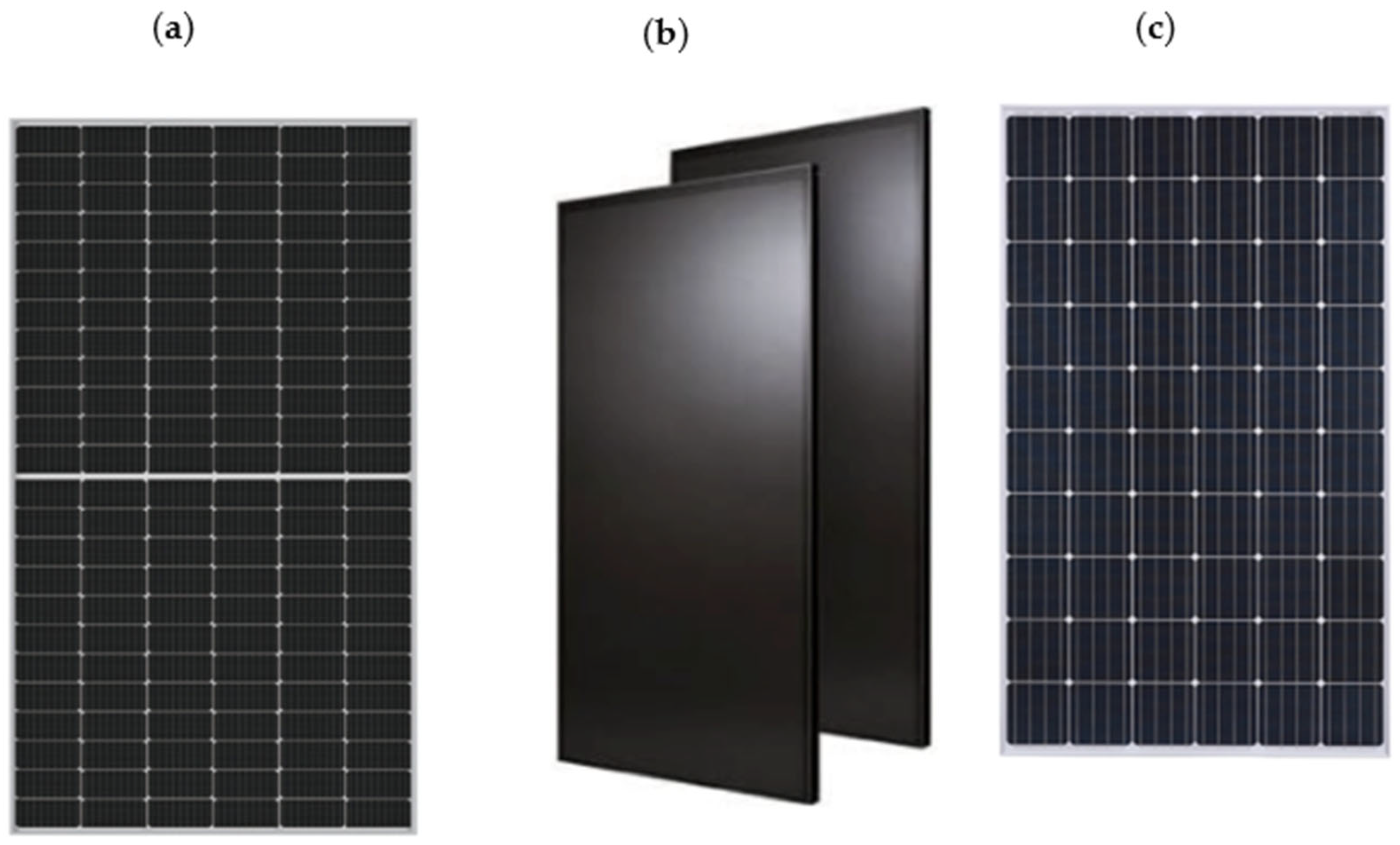
Figure 2.
Large-scale steady-state stationary solar simulator, class AAA.
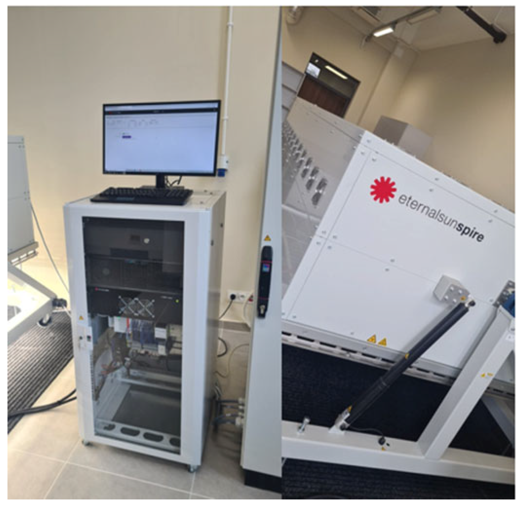
Figure 3.
View of photovoltaic modules during the test.
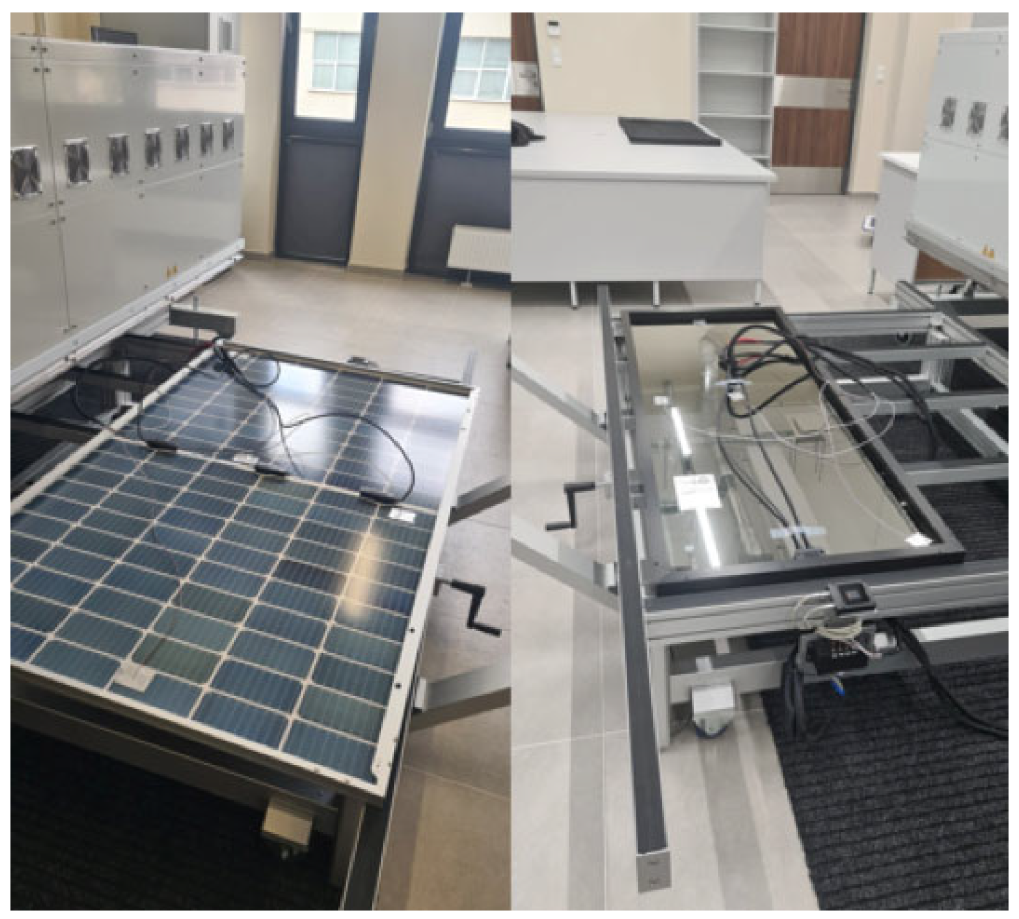
Figure 4.
Graphical representation of artificial neural network (ANN) used in this study: for every data point, the input includes features (green), the hidden layer consists of neurons (blue), and the output of the network is a vector with values and (pink).
Figure 4.
Graphical representation of artificial neural network (ANN) used in this study: for every data point, the input includes features (green), the hidden layer consists of neurons (blue), and the output of the network is a vector with values and (pink).
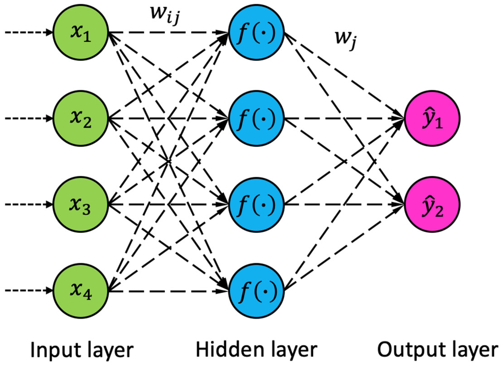
Figure 5.
Flow chart diagram for the data used and processes applied
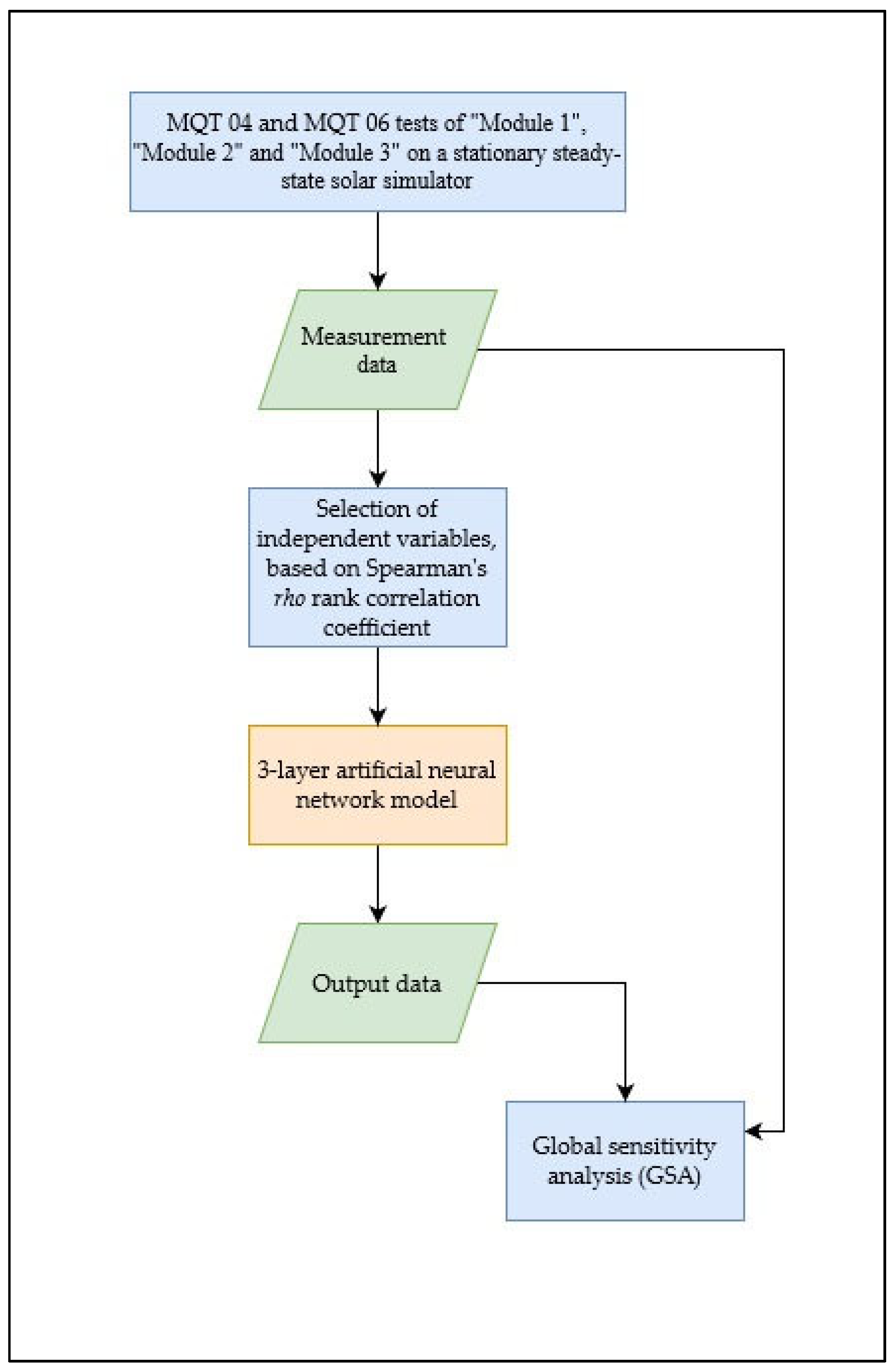
Figure 6.
Summary I-V characteristics of “Module 1”.
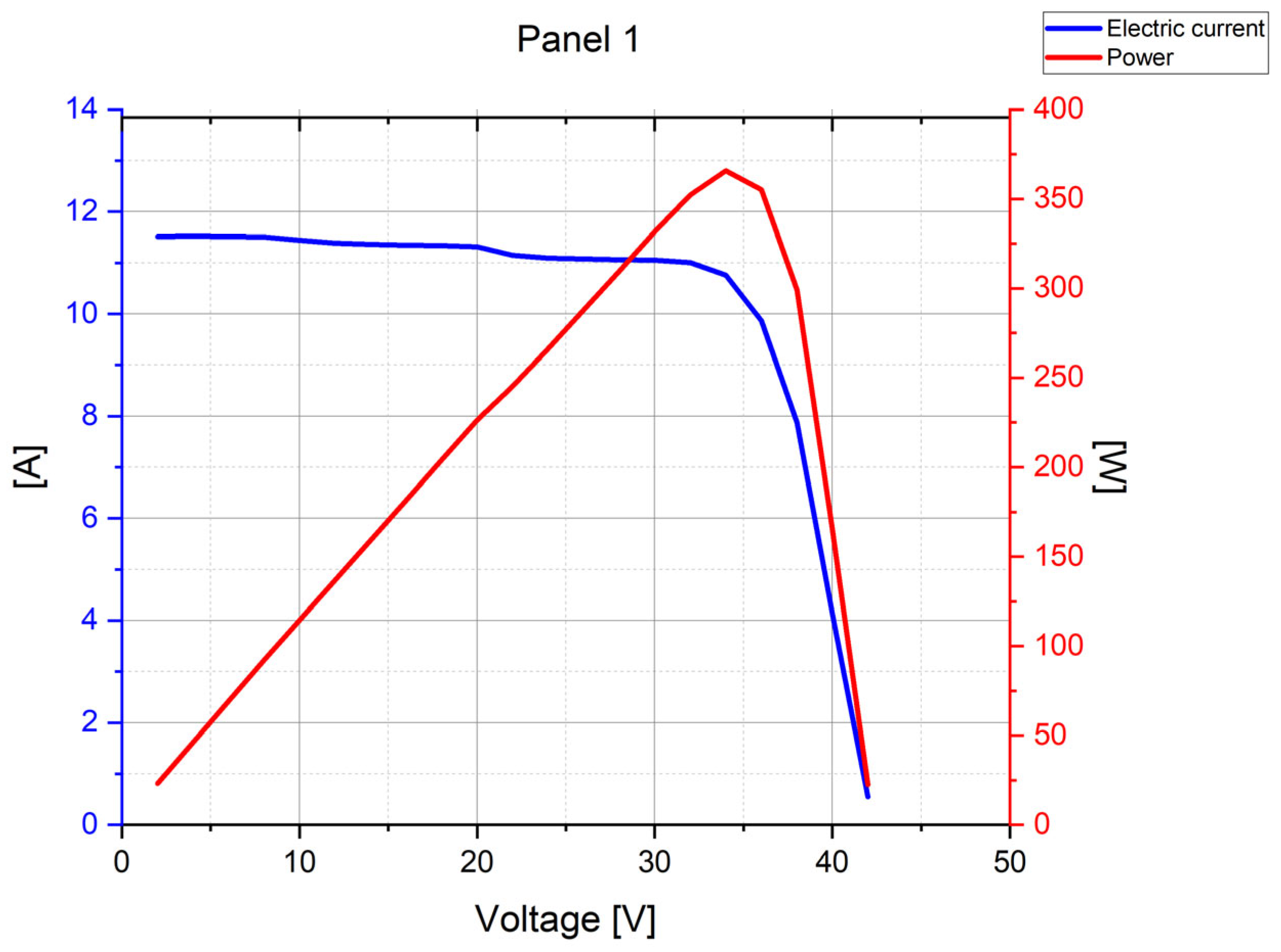
Figure 7.
Summary I-V characteristics of “Module 2”.
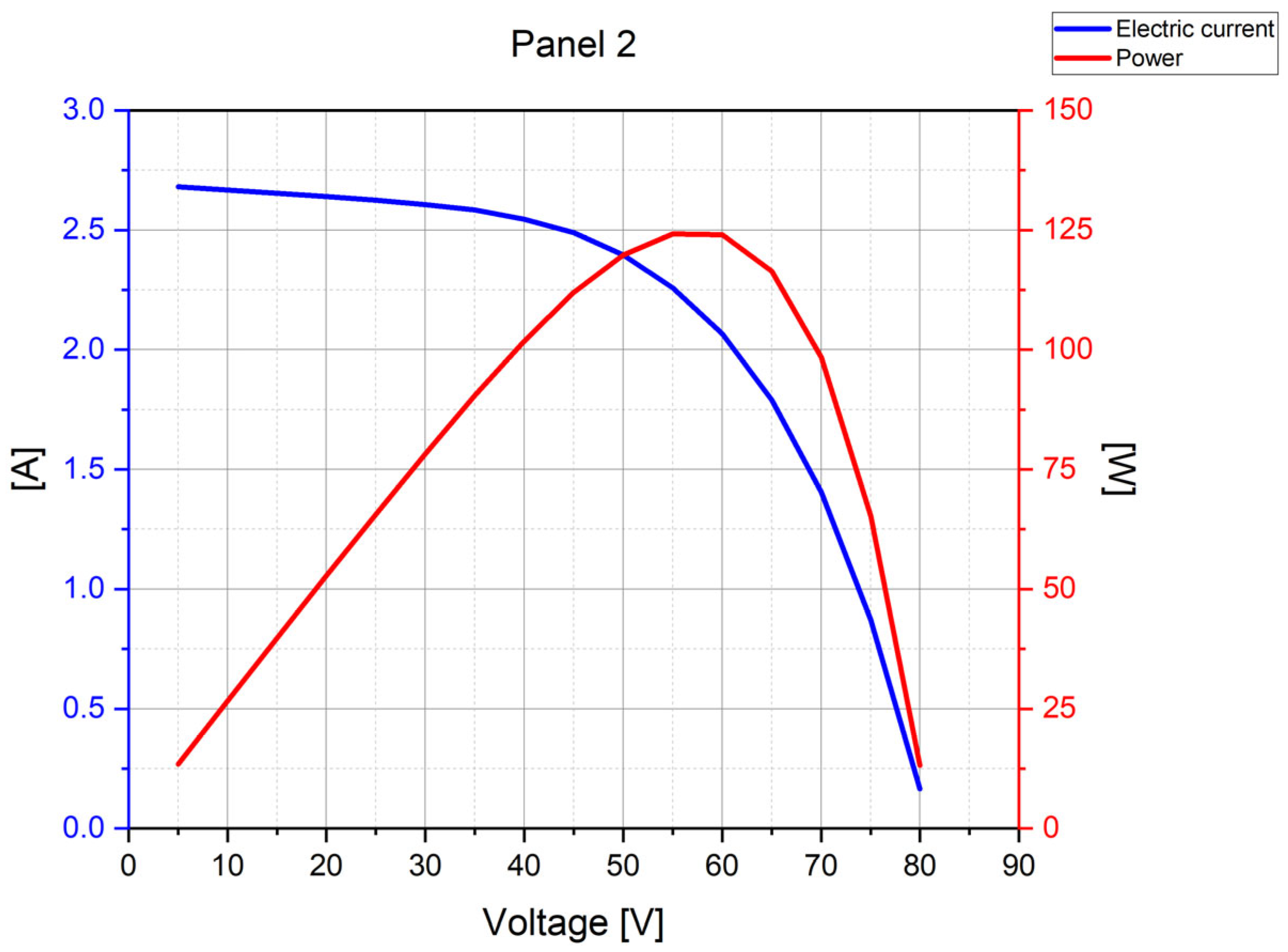
Figure 8.
Summary I-V characteristics of “Module 3”.
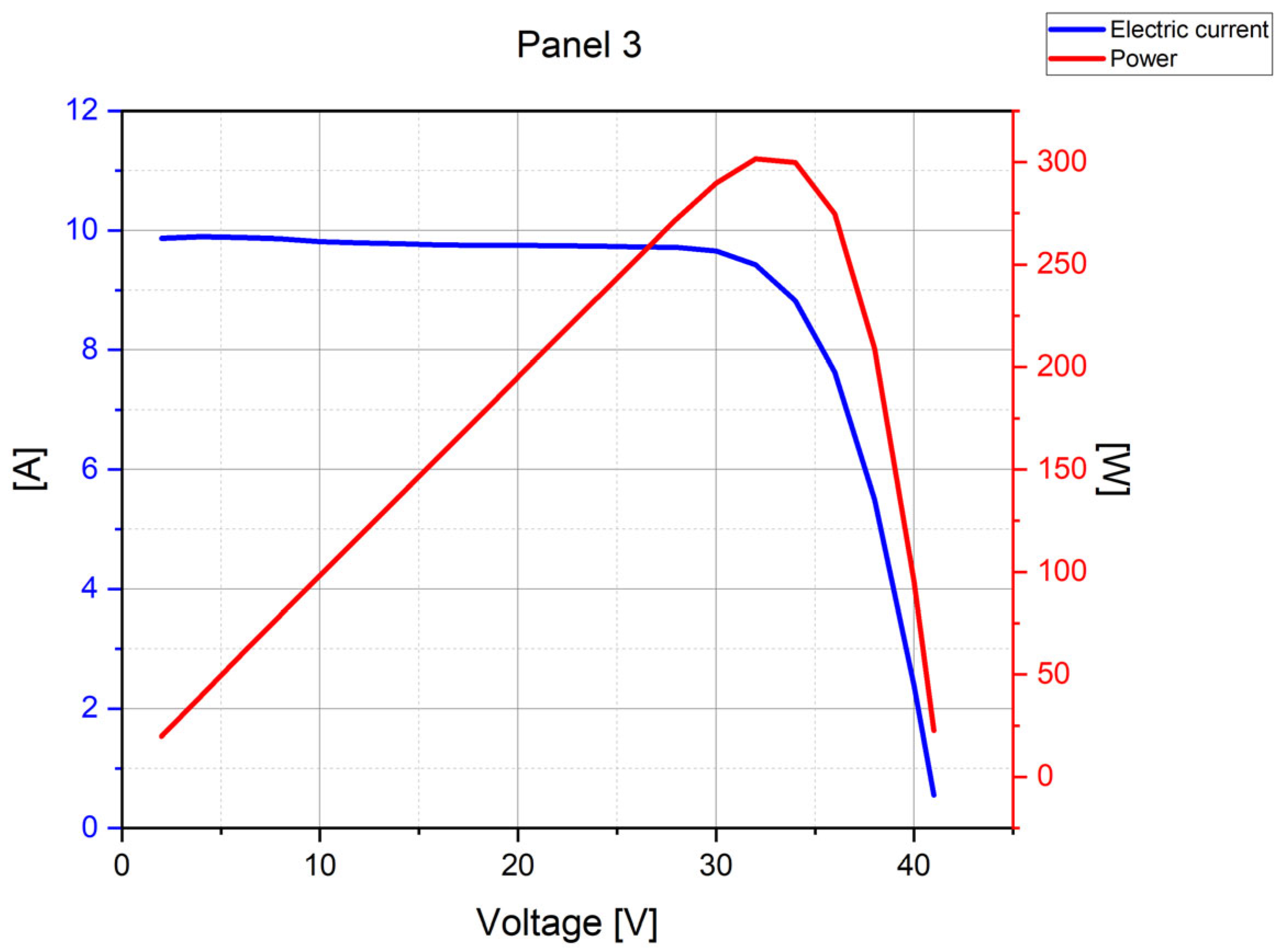
Figure 9.
Comparison of calculated with MLP model and experimentally tested (Measurement) characteristics of the Power [W] and the Voltage [V] for “Module 1” data.
Figure 9.
Comparison of calculated with MLP model and experimentally tested (Measurement) characteristics of the Power [W] and the Voltage [V] for “Module 1” data.
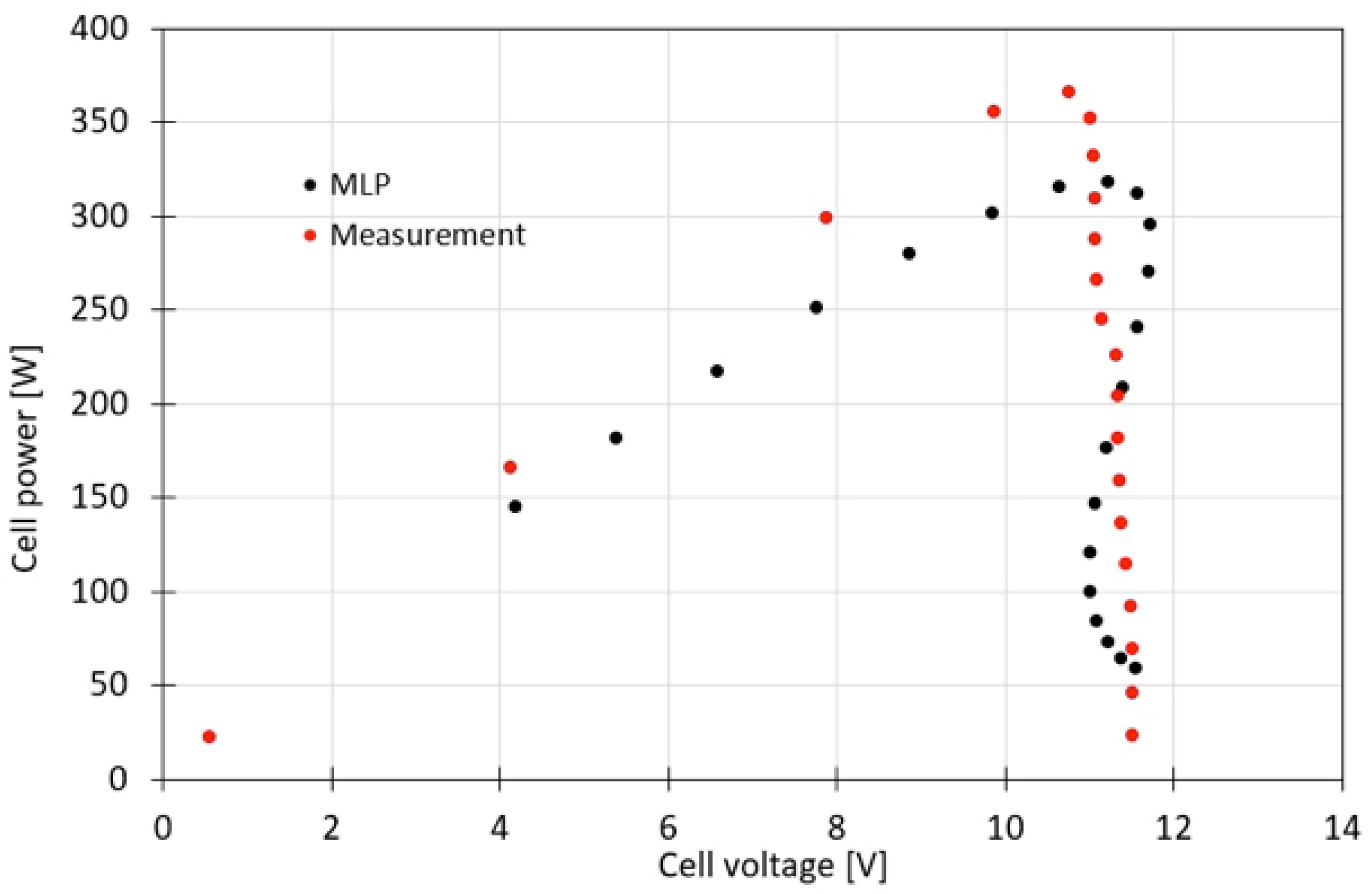
Figure 10.
Comparison of calculated with MLP model and experimentally tested (Measurement) characteristics of the Power [W] and the Voltage [V] for “Module 2” data.
Figure 10.
Comparison of calculated with MLP model and experimentally tested (Measurement) characteristics of the Power [W] and the Voltage [V] for “Module 2” data.
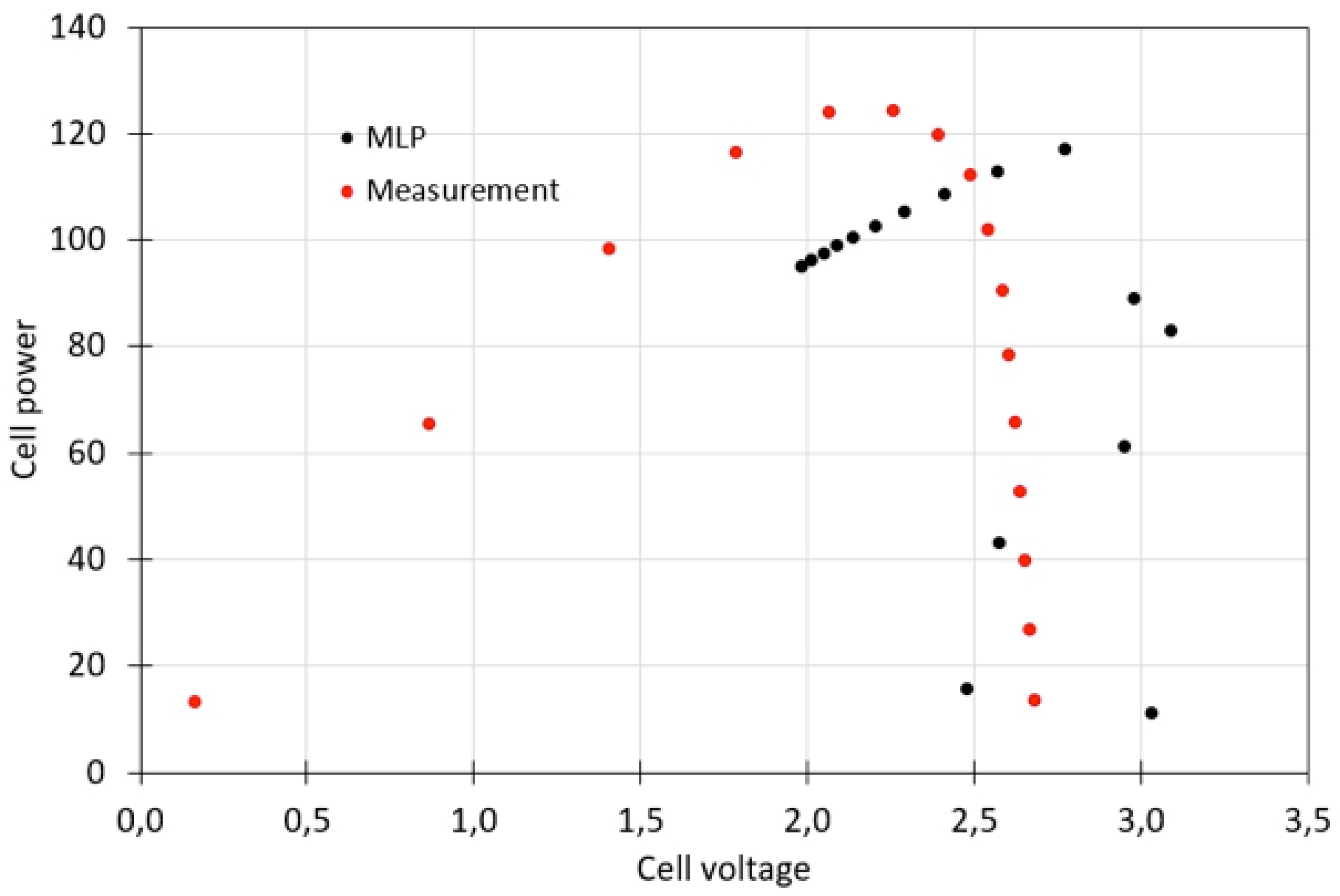
Figure 11.
Comparison of calculated with MLP model and experimentally tested (Measurement) characteristics of the Power [W] and the Voltage [V] for “Module 3” data.
Figure 11.
Comparison of calculated with MLP model and experimentally tested (Measurement) characteristics of the Power [W] and the Voltage [V] for “Module 3” data.
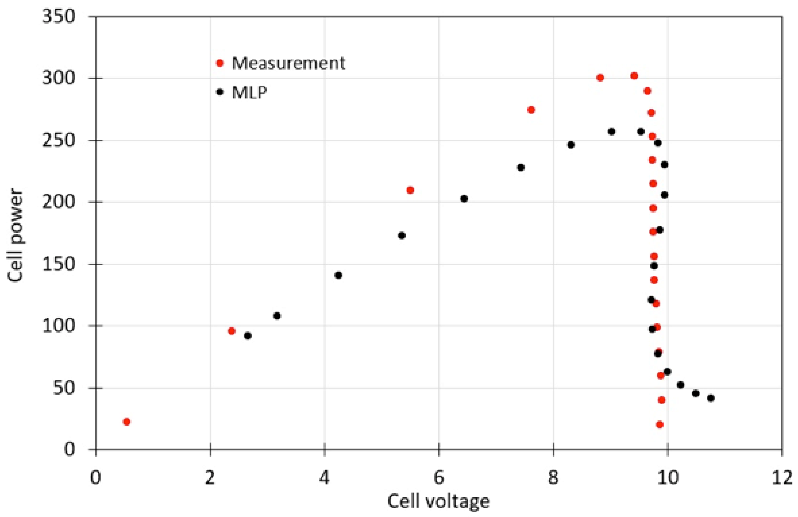

Table 1.
Characteristics of the tested photovoltaic modules.
| Parameter | PV modules tested | ||||
|---|---|---|---|---|---|
| Module 1 | Module 2 | Module 3 | |||
| Max Power | Pmax | [W] | 365 | 145 | 315 |
| Idle voltage | Voc/V | [V] | 40.7 | 59.5 | 40.53 |
| Module efficiency | Eff | [%] | 20.0 | 13.3 | 19.3 |
| Max power voltage | Vmpp | [V] | 34.1 | 60.4 | 33.2 |
| Max power current | Impp | [A] | 10.7 | 2.4 | 9.5 |
| Short-circuit current | Isc | [A] | 11.4 | 2.7 | 10.0 |
| Open-circuit voltage | Voc | [V] | 40.7 | 85.2 | 40.5 |
Table 2.
Results of module parameters obtained during measurements.
| Parameter | Module 1 | Module 2 | Module 3 |
|---|---|---|---|
| Pmax [W] | 367.302 | 125.332 | 303.844 |
| Isc [A] | 11.454 | 2.692 | 9.818 |
| Voc [V] | 44.996 | 86.334 | 49.71 |
| Impp [A] | 10.654 | 2.166 | 9.192 |
| Vmpp [V] | 34.47 | 57.804 | 32.838 |
| Filling Factor [-] | 0.712 | 0.538 | 0.622 |
Table 3.
Dependence of current and power values with averages for tested PV modules.
| Measurement | 5V | 15V | 25V | 35V | 40V |
|---|---|---|---|---|---|
| “Module 1” | |||||
| Power | |||||
| Measurement 1 [W] | 57.8901 | 171.1275 | 275.1322 | 365.42124 | 161.8382 |
| Measurement 2 [W] | 57.6934 | 170.9794 | 274.2930 | 362.1189 | 169.96 |
| Measurement 3 [W] | 57.3698 | 169.8569 | 280.7647 | 361.1334 | 168.7743 |
| Measurement 4 [W] | 57.5227 | 169.8666 | 281.0866 | 359.4855 | 161.9976 |
| Measurement 5 [W] | 57.3990 | 169.6859 | 274.4320 | 354.4239 | 165.2108 |
| Average [W] | 57.57503 | 170.3033 | 277.1417 | 360.5166 | 165.5562 |
| Current | |||||
| Measurement 1 [A] | 11.5763 | 11.409 | 11.0057 | 10.452 | 4.0459 |
| Measurement 2 [A] | 11.5389 | 11.399 | 10.9726 | 10.3584 | 4.249 |
| Measurement 3 [A] | 11.4748 | 11.325 | 11.2311 | 10.3311 | 4.2193 |
| Measurement 4 [A] | 11.507 | 11.3253 | 11.2439 | 10.2844 | 4.0499 |
| Measurement 5 [A] | 11.4799 | 11.3129 | 10.978 | 10.1403 | 4.1303 |
| Average [A] | 11.5154 | 11.3543 | 11.0863 | 10.3132 | 4.1389 |
| “Module 2” | |||||
| Power | |||||
| Measurement 1 [W] | 13.4401 | 65.8343 | 113.0481 | 119.1181 | 17.9283 |
| Measurement 2 [W] | 13.3214 | 65.1509 | 111.2806 | 114.9977 | 11.3292 |
| Measurement 3 [W] | 13.4363 | 65.8609 | 112.2522 | 116.6261 | 10.9828 |
| Measurement 4 [W] | 13.3855 | 65.2238 | 111.2941 | 115.5224 | 13.8337 |
| Measurement 5 [W] | 13.4530 | 65.9243 | 112.1763 | 115.5607 | 11.9393 |
| Average [W] | 13.4073 | 65.5988 | 112.0102 | 116.3650 | 13.2026 |
| Current | |||||
| Measurement 1 [A] | 2.6882 | 2.6334 | 2.5122 | 1.8326 | 0.2241 |
| Measurement 2 [A] | 2.6644 | 2.606 | 2.4729 | 1.7692 | 0.1416 |
| Measurement 3 [A] | 2.6873 | 2.6344 | 2.4945 | 1.7942 | 0.1373 |
| Measurement 4 [A] | 2.677 | 2.609 | 2.4732 | 1.777 | 0.1729 |
| Measurement 5 [A] | 2.6906 | 2.637 | 2.4928 | 1.7778 | 0.1492 |
| Average [A] | 2.6815 | 2.624 | 2.4891 | 1.7902 | 0.165 |
| “Module 3” | |||||
| Power | |||||
| Measurement 1 [W] | 49.4636 | 146.4109 | 243.2909 | 296.5507 | 107.8788 |
| Measurement 2 [W] | 49.5614 | 146.6602 | 243.8605 | 286.7913 | 89.9354 |
| Measurement 3 [W] | 49.5627 | 146.8454 | 243.7230 | 288.4221 | 102.8483 |
| Measurement 4 [W] | 49.4132 | 146.5157 | 242.7928 | 281.0666 | 84.2467 |
| Measurement 5 [W] | 49.2112 | 146.1223 | 242.8360 | 283.3992 | 92.6678 |
| Average [W] | 49.4424 | 146.5109 | 243.3006 | 287.2460 | 95.5154 |
| Current | |||||
| Measurement 1 [A] | 9.8910 | 9.7619 | 9.7318 | 8.4882 | 2.6970 |
| Measurement 2 [A] | 9.9170 | 9.7782 | 9.7545 | 8.2108 | 2.2484 |
| Measurement 3 [A] | 9.9121 | 9.7907 | 9.7494 | 8.2570 | 2.5712 |
| Measurement 4 [A] | 9.8839 | 9.7686 | 9.7121 | 8.0493 | 2.1062 |
| Measurement 5 [A] | 9.8459 | 9.7419 | 9.7138 | 8.1150 | 2.3167 |
| Average [A] | 9.8900 | 9.7683 | 9.7323 | 8.2241 | 2.3879 |
Table 4.
Correlation coefficients of tested PV modules.
| U | Tc | Tp | Pmax | Voc/V | eff | Vmpp | Impp | Isc | |
|---|---|---|---|---|---|---|---|---|---|
| U | 1.00 | 0.73 | 0.25 | 0.33 | 0.33 | 0.33 | 0.33 | 0.33 | 0.33 |
| Tc | 1.00 | 0.29 | 0.79 | 0.33 | 0.79 | 0.33 | 0.79 | 0.79 | |
| Tp | 1.00 | 0.44 | 0.31 | 0.44 | 0.31 | 0.44 | 0.44 | ||
| Pmax | 1.00 | 0.36 | 1.00 | 0.36 | 1.00 | 1.00 | |||
| Voc/V | 1.00 | 0.36 | 1.00 | 0.36 | 0.36 | ||||
| eff | 1.00 | 0.36 | 1.00 | 1.00 | |||||
| Vmpp | 1.00 | 0.36 | 0.36 | ||||||
| Impp | 1.00 | 1.00 | |||||||
| Isc | 1.00 |
Table 5.
Fitting measures between simulation results and measurements on dependent variables.
| Set | Tp | Tc | ||||
|---|---|---|---|---|---|---|
| Training | 0.94 | 24.68 | 36.06 | 0.97 | 0.53 | 1.17 |
| Test | 0.98 | 13.87 | 14.87 | 1.00 | 0.23 | 0.32 |
| Validation | 0.87 | 39.62 | 46.31 | 0.98 | 0.75 | 0.93 |
Disclaimer/Publisher’s Note: The statements, opinions and data contained in all publications are solely those of the individual author(s) and contributor(s) and not of MDPI and/or the editor(s). MDPI and/or the editor(s) disclaim responsibility for any injury to people or property resulting from any ideas, methods, instructions or products referred to in the content. |
© 2024 by the authors. Licensee MDPI, Basel, Switzerland. This article is an open access article distributed under the terms and conditions of the Creative Commons Attribution (CC BY) license (http://creativecommons.org/licenses/by/4.0/).
Copyright: This open access article is published under a Creative Commons CC BY 4.0 license, which permit the free download, distribution, and reuse, provided that the author and preprint are cited in any reuse.


