
Submitted:
19 May 2025
Posted:
20 May 2025
You are already at the latest version
Abstract
The addition of battery storage to solar plants enhances the ability of those plants to deliver electricity during high-value periods. However, the value proposition of storage improves over time due to falling battery costs and increasing volatility in electricity prices, making it unclear when storage adoption should occur. In this work, we consider a 100 MW solar plant constructed in the year 2022 and build a techno-economic model to determine the optimal system design and timing of storage additions in four locations (CAISO, NYISO, ERCOT, and PJM). We find that the optimal time to add storage is in the 2027-2032 timeframe, and that the optimal quantity of storage is much higher than the amount selected if storage is included during the solar plant construction. Additionally, the model suggests significant upscaling in inverter capacity, allowing the storage to deliver electricity during brief high-price periods. We also consider the effect of temporary and permanent subsidies for batteries, showing that a long-term subsidy encourages economically optimal delays in storage adoption.
Keywords:
storage
; battery
; solar
; timing
; optimization
; subsidy
1. Introduction
In 2021, the Environmental Protection Agency [1] found that the electric power sector accounted for roughly 25% of the total U.S. greenhouse gas (GHG) emissions. Worldwide, electricity use (residential, commercial, and industrial) accounts for almost 42% of total GHG emissions [2]. Despite this, by 2050 global energy demand is expected to triple [3]. Without the use of low- or zero-carbon production, this increase in electricity generation could significantly increase GHG emissions. Large-scale solar power plants currently represent only 3.9% of US generation but are rapidly being deployed and represent 53% of new generation in 2023 [4], [5].
Solar power has a notable weakness due to intermittency in power generation due to clouds, weather and seasonality. This creates greater volatility for the electricity grid, which must be managed either at the solar facility or by other grid entities [6], [7]. One solution to this volatility is the addition of battery energy storage that is co-located with the solar plant, which allows the solar+storage facility to become a more reliable and dispatchable source of renewable energy [8], [9]. Historically, the use of battery storage solutions was limited due to high battery costs, but this has been changing as those costs decrease, making battery storage more attractive for solar developers. The National Renewable Energy Laboratory (NREL) predicts that battery costs will continue to decrease through 2050 [10].
The importance of affordable renewable energy has led lawmakers to institute federal tax credits for solar power. The tax credit program allows for a plant to capitalize on either an investment tax credit (ITC) (reduces tax liability for a percentage of the solar system cost) or a production tax credit (PTC) (credit per kilowatt-hour kWh of electricity generated by solar technologies for the first 10 years a system is in operation). These credits offer substantial assistance to solar owners and investors, driving extensive investment in the last 10 years [11]. However, the decision to add battery storage to existing or newly built solar plants is more complex. Uncertainty surrounding the operation of solar plus storage plants (due to plant characteristics, grid characteristics, and geographic characteristics) and the predicted declining costs of solar and storage assets can make it difficult to evaluate and justify the upfront cost of adding storage to a solar facility.
Existing research on storage additions to solar plants has identified the potential of storage to mitigate intermittency in solar generation and considered the economic costs and benefits of the investment [12], [13], [14], [15]. In 2010, Nair and Garimella [15] found that battery energy storage has the highest potential revenue but will not be extensively employed until initial capital costs are driven down by policy or demand. Eyer and Corey [13] concur but also mention that there is recognition by policymakers and regulators, who are creating current or emerging incentives that are strong opportunity drivers for storage adoption.
Other work has identified the optimal storage size under different characteristics of a plant, such as weather, electricity consumption, and electricity prices [16], [17], [18]. Arun et al. [16] provide illustrative examples to storage sizing and propose that retaining a high system reliability requires attention to the ambient temperature effect on system sizing. Other work considers where future deployments should be located to ensure they make sense economically, which tend to be those with the best weather patterns and supportive electricity prices, such as California and Texas [19].
Researchers have performed detailed studies of different solar+storage technologies and configurations, determining how to best exploit technologies both behind and in front of the meter [20], [21], [22]. Englberger et al. [20] find that including both AC and DC storage can decrease the required amount of inverters and increase revenue but increases capital costs since batteries are more expensive than inverters. And Montanes et al. [22] conclude that two- to four-hour duration batteries seem to be most economically viable currently and locations like California and Texas should have a 1:1 ratio of battery to generation capacity for highest net value. These are just prominent examples of an extensive body of solar+storage research that considers optimal design from many different perspectives. However, one perspective seems to be missing: When should we add energy storage to a solar power plant? In an era when the costs of storage keep falling and the benefits of better dispatchability of solar output is increasing investigating the optimal timing of storage additions is highly relevant[10], [23].
The net benefit of adding energy storage to a solar plant increases over time due to two factors: the falling cost of batteries and the increasing benefit of electricity dispatchability. The first factor is well-known, but a smaller and growing literature is showing how high-renewables systems will affect electricity system economics. Average electricity prices are likely to fall as the deployment of renewable energy increases, introducing a “revenue cannibalization” effect for investors in wind and solar [15], [19], [24]. There is a wide body of research that studies future pricing, and while this is important, it lacks substantive conclusions as to how to mitigate this phenomenon or how revenue cannibalization can increase the value of storage over time. The focus on decreasing energy prices, especially during the periods when solar/wind are producing, indicates the need for future research to understand how we can continue decarbonizing the grid while ensuring it makes both social and business sense [24], [25].
Prior work on solar+storage has intensively investigated many important questions but has not addressed the issue of optimal timing of battery energy storage for new and existing solar plants. In this work, we directly address this question, using a techno-economic model that combines future energy prices, infrastructure costs, and solar plant design to identify the optimal timing and design of storage additions to solar plants. While investment decisions may currently consider the fact that storage will be lucrative in the future, our work additionally considers how initial solar plant design might prepare for later storage additions by scaling the inverters in an anticipatory way. It may be optimal to construct storage capacity in one or more phases several years after the initial construction of the solar plant. This model identifies the optimal inverter sizing, storage capacity, and construction timing for solar plus storage plants. We run the model with data from four Independent System Operators (ISO’s) to compare the economics of differing locations across the U.S. Furthermore, this model can be utilized to assess policy options, such as the effect of different subsidies quantities and phase-out, and aid in the design of policies that support the adoption of solar plus storage facilities.
2. Materials and Methods
Figure 1 presents an overview of the modeling approach. The model begins by producing a forecast of future electricity prices that uses historical prices from 2017 along with NREL forecasts of wind/solar generation through the year 2050. This results in hourly prices for four ISOs every five years from 2017 through 2047. These future electricity prices are used as an input for a linear programming-based operational model of a solar+storage plant. This module produces the optimal hourly operation of a solar+storage generator, given the size of solar, storage, and inverters, electricity prices, and solar generation patterns, and calculates the annual revenue. A Net Present Value (NPV) model calculates the NPV of a given solar+storage buildout strategy, given the scale and timing of solar, inverter, and storage additions and the estimated annual revenue of operation in each 5-year period. A higher-level optimization module uses the solar+storage operational module and the NPV module to search for NPV-maximizing buildout strategies. For this work, we assume that a 100 MW solar plant will be built in the initial year and allow the model to optimize the quantity of storage, the timing of storage additions (including in year 0), and the initial scale of inverters. Thus, the modeling perspective asks: if you are building a solar plant, how should inverters be initially scaled, when should storage be added, and how much storage would you want to add?
2.1 Data Inputs
Each Independent System Operator (ISO) in the U.S. has its own electricity generation mix, energy price patterns, and solar resource. These factors can contribute to differing optimal solar+storage strategies between locations. For this reason, we perform the analysis for locations in four U.S. ISOs: New York ISO (NYISO), PJM Interconnection (PJM), Electric Reliability Council of Texas (ERCOT), and California ISO (CAISO). For each ISO, we utilize a locational marginal price (LMP) in two different years, 2017 and 2022. The LMP represent the hourly electricity prices in different geographical zones as defined by each ISO. The zonal pricing system is employed by ISO’s to accurately reflect the difference in electricity generation, transmission, and distribution costs in the different zones. Additionally, we collect data on renewable generation capacity from the National Renewable Energy Laboratory (NREL) Electrification Futures Study for each ISO and historical capacity in both of the aforementioned years [26], [27]. Finally, we utilized demand and seasonal regression coefficients from prior research by Das et al. [24] to aid in calculating future LMP values out to the year 2050.
The next level of analysis, the solar plus storage module, utilizes the hourly electricity pricing from the prior level, as well as hourly solar generation patterns taken from Das et al. [24] and the NREL renewable capacities. Additionally, this module receives an initial inverter size, solar capacity, and storage capacity from the higher-level optimization module.
The high-level optimization relies on cost data for solar (per MW) and inverters (per MW), and the time-varying cost of storage (per MWh). Utility-scale solar and inverter costs are taken from NREL’s 2022 annual technology baseline, while the current and future battery storage costs are derived from NREL’s storage futures study [27], [28]. These inputs are given as parameters for the model and are not altered through the optimization.
2.2 Electricity Prices
The modeling approach requires estimates of future hourly electricity price patterns, which are challenging to locate or derive. For this work, we use a simple method to estimate future hourly electricity prices developed by Das et al. [24]. The electricity prices we use include both past and future electricity prices, reflecting model years 2017 (historical), 2022 (historical), 2027, 2032, 2037, 2042, and 2047. Historical electricity prices are monitored and published by ISOs and other third parties which were the sources for our collection of 2017 and 2022 data [29], [30], [31]. We decided to examine both 2017 and 2022 as reference historical years due to the concern that 2022 might include undesirable effects from COVID-19. We recognize that the pandemic may have affected electricity utilization and pricing as well as renewable energy projects, which could skew the pricing data from the normal and expected patterns after the year 2019.
After collection, the 2017 and 2022 electricity pricing data were organized into an hourly time-series by ISO. In the case of LMP pricing that was reported at a higher resolution than hourly, the inter-hour pricing was averaged. Any missing data was interpolated from adjacent data points.
An important input to the model is estimates of future hourly electricity prices. We use the method presented in Das et al. [24] along with forecasts of future wind/solar deployment from the NREL Electrification Futures Study [27]. To predict future electricity prices, we model renewable generation as negative demand and assume that there is a linear relationship between price and renewable generation capacity as determined by Das et al. [24]. To calculate future pricing the following equation was utilized:
LMPnew = LMPref – (Change in Dollar per MW of Renewable Generation * (RenewableGenerationcurrent – RenewableGenerationref)).
The benefit of this method is that it predicts future prices while retaining the realistic hourly fluctuations of observed/historical data. However, this method does not consider large-scale shifts in demand patterns or traditional generation, meaning that it is more accurate for near-term predictions and is likely to be structurally incorrect as the forecast goes further into the future.
A reference year of 2022 was used for the LMP and renewable generation data in Equation 1. The change in dollar per additional MWh of renewable generation represents the linear price decrease informed by the amount of installed renewable energy. These relationships are taken from Das et al. [24], which calculated the effects of changes in demand on price, calculated on a seasonal basis (seasons were defined as February-April, May-July, August-October, and November-January). Estimated hourly wind/solar generation was calculated by multiplying the future capacity in each region (using data from NREL’s Electrification Futures Study):
and hourly capacity factors from Das et al. [24], but originally derived from the Eastern Wind Integration and Transmission Study (EWITS), the Western Wind dataset, and the Typical Meteorological year (TMY3) dataset).
Renewable Generation per Hour = Solar Capacity * Capacity Factor,
It is important to note some benefits and limitations of this price forecasting method. As previously mentioned, by utilizing past pricing data the realistic hourly pricing patterns are preserved into the future, which is not the case for price patterns derived entirely from dispatch models. Additionally, the hourly capacity factors allow our predictions to follow generation patterns observed in recent years. On the other hand, these factors become less pertinent over time, so the estimates will provide diminishing returns over the long term. Given the importance of near-term periods in our NPV calculations, due to discounting, the use of a method that is more relevant for near-term periods seems appropriate.
2.3 Solar Plus Storage Linear Programming Model
The following linear programming is built upon a previous model used for a revenue maximization for a storage-only system [32]:
The objective function, Equation 3, maximizes revenue over the year, where Pt and Et represent the electricity price and the electrical energy delivered from storage at time t, respectively. Et may be negative, indicating energy storage. St represents the state of charge of the storage (in units of energy). Smax is the maximum state of charge, 4-7. The initial state of charge for the storage system is set to 50% of its maximum capacity, Equation 3. Energy transfers into and out of storage are subject to inefficiencies, with losses evenly distributed between the charge and discharge processes, Equation 5-6, where ηrt represents round-trip efficiency. The storage system has constraints on the lower and upper limits of charge, Equation 7-8, between 0 and Smax. The maximum increase in St , Equation 9, is the minimum of Rmax and Gt, which represent the maximum charge/discharge rate of the battery system and solar generation in hour t, respectively. The maximum decrease in St, Equation 10, is the negative minimum of Rmax and the maximum of 0 and Imax – Gt, where Imax represents the inverter capacity.
The linear programming model optimizes along the 8760 timepoints in chunks of 500 hours, with a 10% overlap to minimize boundary effects. Hourly plant operation optimization is only performed in the years 2022, 2027, 2032, 2037, and 2042. Gross projected revenue for in-between years (e.g., 2023, 2024, 2025, 2026) is linearly interpolated between the optimized outputs.
2.4 Net Present Value Model
The middle layer of the model functions to communicate between the user-facing optimization model and the solar+storage operation LP module to generate a lifetime NPV estimate for the plant scenarios. This layer is where the plant investment, battery prices, operations and maintenance, battery salvage, and discounting are handled. Final cash flows are combined by converting all values to 2022 dollars for NPV calculations.
2.4.1 Solar Plant
While the model is capable of varying solar scale and timing, all scenarios in this work assume that a 100 MW fixed-axis solar plant is built in year 0 (2022) of the project. Thus all build scenarios have the same estimated total cost of $94M in 2022 dollars [28].
2.4.2 Inverter Pricing
Inverters were estimated to cost $0.045/Wdc [28]. Inverters are always built during plant construction and are not expanded in later periods. This allows us to see how the anticipation of later storage additions affects the sizing of initial inverter selection.
2.4.3 Battery Pricing
Battery pricing is calculated based on NREL’s 2021 Battery Energy Storage System (BESS) table [27]. Battery types include 2-hr, 4-hr, 6-hr, 8-hr, and 10-hr. Future pricing conditions include low, mid, and high scenarios. Our base case assumes the mid scenario and 2-hour batteries, though power to energy ratio is investigated in sensitivity analysis. Battery additions to the solar plant are limited to a single year, including allowing for year 0 additions, where batteries are installed in the initial project with the solar.
2.4.4 Operations and Maintenance
Yearly plant O&M is estimated to be 1.1% of the capital investment costs. Yearly battery O&M is estimated to be 2.5% of the purchase price of the current active batteries [28].
2.4.5 Capital Payments and Battery Storage
All capital costs are handled as annualized payments over the expected lifetime of the asset, equivalent to an amortized loan with an interest rate of 5.5% for the solar plant and 4.5% for battery storage. This approach was used to address “salvage value” issues relating to the end of the modeling period. The operational lifetime for the solar plant is 25 years, resulting in an annual Capital Recovery Factor (CRF) of 8.55% (7.45% Loan CRF + 1.1% Operations and Maintenance (O&M)). Battery payments are made over the expected lifetime of 15 years, which results in a higher CRF of 11.81% (9.31% Loan CRF + 2.5% OM). Because battery lifetime is shorter than the study period, storage is replaced at end of life with new storage at the prevailing current year (2037 or 2042) market price. Because all costs are paid out at a fixed yearly rate over their lifetime, a salvage value does not need to be estimated.
2.4.6 Discounting
A discount rate of 5% and an inflation rate of 3% are used to calculate NPV.
2.5 Optimization Model
The high-level optimization model searches for NPV-maximizing choices for inverter capacity (built in year 0), storage capacity, and the storage addition year. This optimization is performed in MATLAB, using the global optimization and parallel computing toolboxes. Storage capacity and inverter capacity were constrained to specific ranges, and the possible storage addition years are constrained to 5-year increments between 2022 and 2047, as described in Table 1. A “build” is defined as a single combination of storage capacity, inverter capacity, and storage addition year for a solar plant at a given ISO location. To determine the appropriate range of searchable values for storage capacity and inverter capacity, preliminary testing was performed at a low resolution (~50 builds per additional year, 250 total) until a 25% increase of maximum potential storage capacity did not influence the optimal build conditions. For NY, CA, and PJM, 600 MWh was determined to be appropriate for base case analysis. ERCOT required a significantly higher threshold at 6,000 MWh, in order to not impede storage optimization. The maximum search range for inverter capacity was set at 2/3rds of the maximum potential storage capacity, as this provided more than adequate coverage while improving the optimization resolution.
Optimization within the specified solution space was performed with a genetic algorithm search, available within MATLAB’s global optimization toolbox. Each condition (e.g., base case, subsidy) began with a 25-generation optimization over the total range of storage, inverters, and storage addition years. Since the genetic algorithm favors higher performing regions of the solution space over lower performing areas, storage addition years with relatively lower NPV were underrepresented by the search (~10:1 in number of builds). To improve the resolution within these suboptimal storage addition years, an additional 5-10 generations of optimization were run in each underrepresented storage addition year. Final NPV estimates for a given set of conditions were not strongly influenced by the initial conditions, suggesting good convergence (see supplementary data). Over 1.2 million potential build combinations were possible for each set of conditions, making a brute-force search computationally infeasible. However, validation testing found that each dimension was smooth and contained only one maximum. Given the smooth nature of the optimization landscape, 0.5% of potential combinations (~6000) is sufficient for the genetic algorithm to obtain precise results that are reliably chosen as optimal during repeat runs with the same conditions.
3. Results
3.1 Base Case by Region
The base case analysis assumes certain fixed parameters across the four studied regions: 100 MW of solar built in year 0 (2022), 2-hour power-to-energy ratio for batteries, and the NREL mid-price scenario for battery cost projections. The decision variables that are being optimized are the initial inverter scaling in year 0, the quantity of energy storage to add, and the year in which to add it. The base case results are shown in Table 2.
In the base case scenario, all four regions show a positive NPV over the 25-year operational period of the plant, meaning that a solar+storage project is expected to be profitable. Additionally, all four regions choose to add storage at some point, showing that storage is an appropriate investment that improves upon the solar-only NPV. In anticipation of storage, all four locations install excess inverter capacity in anticipation of later storage. In practice, the economically optimal design for most solar facilities uses an undersized inverter system (i.e., 100 MW of solar panels would be linked to less than 100 MW of inverter [33]. However, our model chooses to significantly oversize the inverters for the 100 MW solar facility, but this only lasts 5 to 10 years until storage is added and the higher inverter capacity is needed. This choice makes financial sense because of the low cost of inverters relative to both solar and storage, meaning that the preparation cost is small. The storage addition year in the base case is in the 2027-2032 timeframe in all four locations, suggesting that storage additions are more preferable in future years than upon solar plant construction, at least with the base case assumptions. The ERCOT results suggest adding storage in the year 2027, the earliest timing in our analysis, which may be because of the higher value of storage under ERCOT price patterns. The optimal storage and inverter capacities for ERCOT are significantly larger than that of the other regions, showing that the model sees this as an opportunity to build a profitable and large storage facility co-located with the solar plant. Finally, regions with decreased utilization of storage tend to have lower plant NPV and quantity of inverters, presumably because limited market benefits of storage limit both factors.
3.2 Forced Storage Build Year Analysis
The model can be used to consider the possibility of adding storage in any year in the studied timeframe. By comparing and understanding how the optimal storage and inverter capacities change with build year and how that change affects NPV of the plant, we can better understand why the model identifies 2027 to 2032 as the optimal choice for storage additions. For this set of results, we force particular build years for storage and let the model choose the optimal quantity of storage and the initial inverter scale. For comparison, we also include a solar-only scenario where no storage is permitted in any year, though inverter scale is optimized. This forced storage build year analysis was performed for all four regions under otherwise base case conditions. Figure 2 depicts the results for CAISO. Figure 3 depicts the results for ERCOT. Figure 4 depicts the results for NYISO. Figure 5 depicts the results for PJM.
For CAISO, all of the storage scenarios have higher NPV than the solar-only comparison. The optimal amount of storage is approximately four times higher if storage is added 5 or 10 years after the solar. Even with cheaper storage, this still represents an increased total investment in batteries but represents a kind of tipping point where the marginal benefit of more storage becomes slightly higher than the marginal cost until much higher levels of storage are reached. In this way, moderate changes in the cost of storage can result in a significant shift in the optimal system design, as observed previously for other electricity systems (Sandler et al., 2021). The optimal inverter capacity has a slight upwards trend, following the optimal quantity of storage. Inverters are inexpensive compared with solar and storage, so this increased inverter capacity is built in anticipation of later storage and allows storage to better time-shift electricity production to specific valuable hours.
ERCOT also shows an increased NPV for storage added in any operational year, with an optimal build year of 2027. ERCOT electricity prices are the most volatile of the four studied locations, presumably due to the energy-only structure of the electricity market, and storage is naturally profitable under these conditions. Thus, the model chooses much larger amounts of storage than in other regions, with storage able to hold several days of solar production. This is true even though the storage can only be charged from the co-located solar, and it uses storage to save up solar energy and deliver it in bulk during specific high-price hours. These observations are consistent with the real-world deployment of a large number of battery facilities in ERCOT, both co-located with solar and as stand-alone sites [34].
NYISO had the overall lowest NPV results across the board. The addition of storage only improves NPV starting in 2027, with an optimal build year of 2032. Like other locations, the optimal amount of inverters increases in the first few periods then falls towards the end of the study period. This is because of the end-of-study cutoff for NPV: across all scenarios, a greater quantity of inverters is associated with greater quantity of storage, as it enables faster discharge of batteries in high-value hours. But if storage is added in the last 5-10 years of the solar plant, the overall benefit of that synergy with storage is limited to a short period and overbuilding inverters in the initial plant design is less desirable.
PJM performed similarly to NYISO but has a higher overall NPV. PJM offers a greater NPV than NYISO without storage and the model recommends building more inverters and storage than in NYISO and generates a greater NPV.
3.3 Simple Fixed Subsidy
Similarly, we analyzed a fixed subsidy rate on the plant NPV to determine its effectiveness. Currently, the U.S. investment subsidy provides a 30 percent discount on equipment, as described in section 1. Figure 6 shows the simulated effect of a 30% fixed subsidy on storage investment costs.
Three scenarios were tested in CAISO over the standard operational period: no subsidy (control), an expiring 30% battery subsidy that only provides benefits in 2022, and a fixed 30% battery subsidy that lasts the entire operational period. As expected, the presence of the subsidy increases the projected NPV and optimal storage capacity of the solar plus storage system. The increase in both projected NPV and storage capacity was larger in the fixed subsidy case than the expiring subsidy case, despite the subsidies having equivalent magnitude during the initial build in 2022. This is due to the replacement costs of the batteries also being subsidized over the operational period in the fixed subsidy case, whereas the batteries are replaced at full price in the expiring case. Since the plant cannot downsize its storage capacity in future years, a more modest quantity of batteries is built in 2022 when the subsidy is expected to expire.
3.4 Battery Cost Projection Sensitivity Analysis
We also assess the effect of future battery prices on the optimal scale of deployment, shown in Figure 7. Future battery pricing is separated into three levels offered in the NREL projections that were used: low, mid, and high. Mid corresponds to the middle future pricing prediction by NREL (our base case), low represents a low-cost scenario, and high represents their high-cost scenario.
As expected, given the results from the subsidy analysis, the low pricing condition (which corresponds to lower future prices of batteries) significantly increased the optimal quantity of storage in future build years compared to the mid and high conditions. The mid- and high-price scenarios have a similar amount of storage, demonstrating the general value of storage for future solar plants even under higher prices. However, the high-price scenarios had notably lower NPV than the mid-price results (not shown) because of the cost of the batteries.
3.5 Battery Charge/Discharge Rate Sensitivity Analysis
A sensitivity analysis was performed for the CAISO location to assess the effect of battery charge/discharge rate on optimal build parameters, shown in Figure 8. The 4-hr discharge rate performed the best in terms of maximized NPV, closely followed by the 6-hr condition. The 2-hr batteries performed better than the 8-hr batteries in the near years (2022-2027), but 8-hr batteries overtook the 2-hr battery from 2028. Predictably, with faster battery charge/discharge rates, more inverters and less total storage capacity was required to capitalize on hourly electricity price fluctuations.
4. Discussion
In this work, we used a combined linear programming and net present value approach to determine the optimal solar plant design choices as a function of battery properties and the timing of battery additions. While each scenario had its own results, there are several consistent themes that we observe. First, the addition of batteries at some point in time improves the NPV of the solar plant across scenarios and assumptions. If storage is added during the construction of the plant (in 2022), only two of the four locations - CAISO and ERCOT - show an NPV benefit. This is consistent with observed market behavior, as current electricity price patterns and anticipated growth in renewables make California and Texas the top two states for storage adoption in 2023 (Martucci, 2025). While the solar plants in PJM and NYISO don’t show a net benefit for storage in 2022, all four ISOs examined enjoy net benefits from storage starting in the year 2027.
The second general result is that the optimal time to add storage to a solar plant built in 2022 is consistently 5 to 10 years in the future. These results suggest that there is a value, sometimes a significant one, for solar developers and plant owners in planning for future storage additions and integration. This may imply physical preparation, such as leaving space for battery enclosures within the facility or sizing inverters based on future needs rather than for optimal solar-only design. Preparation could also be financial or contractual, such as ensuring funding during plant construction for future battery additions.
A third general result is that the addition of DC-connected batteries prompts the addition of more inverters, which we were not expecting. Because batteries are able to absorb excess solar energy, they reduce or eliminate “inverter clipping”, the curtailed energy lost during periods when solar DC output exceeds the available inverters. Thus, our initial hypothesis was that batteries would allow for lower investment in inverter capacity and decrease inverters relative to a solar-only facility. However, due to the low cost of inverters and the high value of electricity in certain hours, the opposite strategy has greater net benefits: batteries allow you to deliver larger quantities of energy concentrated into periods of high prices, which requires scaling up the inverter capacity.
The base case results suggest that waiting to install batteries is consistently preferable to adding them when the plant is built, but this is somewhat contradicted by the fact that current solar plants sometimes include storage. There are practical reasons for this choice that we do not capture in the modeling. In standard solar development practice, a solar developer specifies a project design, contacts an off-taker for the energy, and secures project finance before construction. This process necessitates a specific “bankable” project and any uncertainty about future project modifications would complicate or threaten the ability to close on the project. A second practical issue is that our model does not apply additional costs to having multiple project phases. In reality, there would likely be additional soft costs to delaying the battery construction by 5 or 10 years, such as identifying new financing or engaging a second engineering firm. These practical considerations push developers to design and build the entire project at one time and can explain why our model outputs might differ from current practice. However, there are also additional benefits in terms of real options. By deferring the decision to add batteries, the plant owner will be able to choose the preferred scale and timing of batteries based on improved information about electricity trends and battery prices. For example, waiting 5 years to add batteries allows the owner to either add a larger-than-planned battery if electricity prices are more volatile than expected or to defer the battery addition by another 2 years if battery prices do not fall as quickly as expected.
In the CAISO-focused analysis of subsidies, we observe that both temporary and permanent subsidies result in increased quantities of storage adoption. However, the optimal quantity of storage is higher (550 MWh versus 440 MWh) and occurs sooner (2027 versus 2032) when storage subsidies are expected to persist into the future. This demonstrates the value of long-term policy certainty in supporting the storage and solar industries. In the case where a solar developer expects that the policy support will end soon, they are more likely to add storage immediately, which is sub-optimal and results in significantly less storage in total (300 MWh versus 550 MWh). Long-term policy certainty would enable developers to plan for later additions of storage, which our analysis finds to be economically optimal.
Author Contributions
Conceptualization, E.H.; methodology, A.H., J.K., E.H; software, A.H., J.K.; analysis, J.K., A.H.; data curation, J.K.; writing, J.K., A.H., E.H.; visualization, J.K., A.H.; supervision, E.H. All authors have read and agreed to the published version of the manuscript.
Funding
This research received no external funding.
Data Availability Statement
The raw data and code supporting the conclusions of this article will be made available by the authors on request. Much of the original data comes from publicly-available data sources, described above in the Materials and Methods section.
Acknowledgments
During the preparation of the linear programming code, the author(s) used ChatGPT 3, 3.5, 4o for the purposes of debugging and data cleaning. The authors have reviewed and edited the output and take full responsibility for the content of this publication.
Conflicts of Interest
The authors declare no conflicts of interest.
References
- U.S. Environmental Protection Agency, “Sources of Greenhouse Gas Emissions.” Accessed: Apr. 26, 2025. [Online]. Available: https://www.epa.gov/ghgemissions/sources-greenhouse-gas-emissions.
- H. Ritchie, “Sector by sector: where do global greenhouse gas emissions come from?,” Our World in Data, Sep. 2020, Accessed: Apr. 26, 2025. [Online]. Available: https://ourworldindata.org/ghg-emissions-by-sector.
- IRENA, “World Energy Transitions Outlook 2023: 1.5C Pathway, Volume 1,” International Renewable Energy Agency, Jun. 2023. [Online]. Available: https://www.irena.org/-/media/Files/IRENA/Agency/Publication/2023/Jun/IRENA_World_energy_transitions_outlook_2023.pdf.
- Solar Energy Industries Association, “Solar Market Insight Report 2023 Year in Review,” SEIA. Accessed: Apr. 26, 2025. [Online]. Available: https://seia.org/research-resources/solar-market-insight-report-2023-year-review/.
- U.S. Energy Information Administration, “Electric Power Monthly: 24.” Accessed: Apr. 26, 2025. [Online]. Available: https://www.eia.gov/electricity/monthly/archive/december2024.pdf.
- C. H. B. Apribowo, S. Sarjiya, S. P. Hadi, and F. D. Wijaya, “Optimal Planning of Battery Energy Storage Systems by Considering Battery Degradation due to Ambient Temperature: A Review, Challenges, and New Perspective,” Batteries, vol. 8, no. 12, p. 290, Dec. 2022. [CrossRef]
- M. Ohrelius, M. Berg, R. Wreland Lindström, and G. Lindbergh, “Lifetime Limitations in Multi-Service Battery Energy Storage Systems,” Energies, vol. 16, no. 7, p. 3003, Mar. 2023. [CrossRef]
- A. F. M. Correia, P. Moura, and A. T. De Almeida, “Technical and Economic Assessment of Battery Storage and Vehicle-to-Grid Systems in Building Microgrids,” Energies, vol. 15, no. 23, p. 8905, Nov. 2022. [CrossRef]
- M. Lee, J. Park, S.-I. Na, H. S. Choi, B.-S. Bu, and J. Kim, “An Analysis of Battery Degradation in the Integrated Energy Storage System with Solar Photovoltaic Generation,” Electronics, vol. 9, no. 4, p. 701, Apr. 2020. [CrossRef]
- W. Cole and A. Karmakar, “Cost Projections for Utility-Scale Battery Storage: 2023 Update,” NREL/TP--6A40-85332, 1984976, MainId:86105, Jun. 2023. [CrossRef]
- The White House, “FACT SHEET: Biden-Harris Administration Announces New Clean Energy Projects to Revitalize Energy Communities, Support Coal Workers, and Reduce Reliance on Competitors Like China,” Apr. 2023. [Online]. Available: https://bidenwhitehouse.archives.gov/briefing-room/statements-releases/2023/04/04/fact-sheet-biden-harris-administration-announces-new-clean-energy-projects-to-revitalize-energy-communities-support-coal-workers-and-reduce-reliance-on-competitors-like-china/.
- N. Edoo and R. T. F. Ah King, “Techno-Economic Analysis of Utility-Scale Solar Photovoltaic Plus Battery Power Plant,” Energies, vol. 14, no. 23, p. 8145, Dec. 2021. [CrossRef]
- J. Eyer and G. Coery, “Energy Storage for the Electricity Grid: Benefits and Market Potential Assessment Guide,” SAND2010-0815, Oct. 2023. [Online]. Available: https://www.energy.gov/sites/prod/files/2016/10/f33/sandia_energy_storage_report_sand2010-0815_Feb_2010.pdf.
- V. V. Kuvshinov, V. P. Kolomiychenko, E. G. Kakushkina, L. M. A. Ali, and V. V. Kuvshinova, “Storage System for Solar Plants,” Appl. Sol. Energy, vol. 55, no. 3, pp. 153–158, May 2019. [CrossRef]
- N.-K. C. Nair and N. Garimella, “Battery energy storage systems: Assessment for small-scale renewable energy integration,” Energy and Buildings, vol. 42, no. 11, pp. 2124–2130, Nov. 2010. [CrossRef]
- P. Arun, R. Banerjee, and S. Bandyopadhyay, “Optimum sizing of photovoltaic battery systems incorporating uncertainty through design space approach,” Solar Energy, vol. 83, no. 7, pp. 1013–1025, Jul. 2009. [CrossRef]
- L. Barra, S. Catalanotti, F. Fontana, and F. Lavorante, “An analytical method to determine the optimal size of a photovoltaic plant,” Solar Energy, vol. 33, no. 6, pp. 509–514, 1984. [CrossRef]
- M. Yao and X. Cai, “Energy Storage Sizing Optimization for Large-Scale PV Power Plant,” IEEE Access, vol. 9, pp. 75599–75607, 2021. [CrossRef]
- E. Loth, “Wind energy value and deep decarbonization design, what’s next?,” Next Energy, vol. 1, no. 4, p. 100059, Dec. 2023. [CrossRef]
- S. Englberger, A. Jossen, and H. Hesse, “Unlocking the Potential of Battery Storage with the Dynamic Stacking of Multiple Applications,” Cell Reports Physical Science, vol. 1, no. 11, p. 100238, Nov. 2020. [CrossRef]
- J. McLaren, N. Laws, K. Anderson, N. DiOrio, and H. Miller, “Solar-plus-storage economics: What works where, and why?,” The Electricity Journal, vol. 32, no. 1, pp. 28–46, Jan. 2019. [CrossRef]
- C. C. Montañés, W. Gorman, A. D. Mills, and J. H. Kim, “Keep it short: Exploring the impacts of configuration choices on the recent economics of solar-plus-battery and wind-plus-battery hybrid energy plants,” Journal of Energy Storage, vol. 50, p. 104649, Jun. 2022. [CrossRef]
- D. Feldman, K. Dummit, J. Zuboy, and R. Margolis, “Spring 2023 Solar Industry Update [Slides],” NREL/PR--7A40-86215, 1974994, MainId:86988, Apr. 2023. [CrossRef]
- S. Das, E. Hittinger, and E. Williams, “Learning is not enough: Diminishing marginal revenues and increasing abatement costs of wind and solar,” Renewable Energy, vol. 156, pp. 634–644, Aug. 2020. [CrossRef]
- K. C. Divya and J. Østergaard, “Battery energy storage technology for power systems—An overview,” Electric Power Systems Research, vol. 79, no. 4, pp. 511–520, Apr. 2009. [CrossRef]
- S. Koebrich et al., “2017 Renewable Energy Data Book Including Data and Trends for Energy Storage and Electric Vehicles,” DOE/GO-102019-5113, Jan. 2019. [Online]. Available: https://www.nrel.gov/docs/fy19osti/72170.pdf.
- C. Murphy et al., “Electrification Futures Study: Scenarios of Power System Evolution and Infrastructure Development for the United States,” National Renewable Energy Laboratory, Golden, CO, Technical Report NREL/TP-6A20-72330, Jan. 2021. [Online]. Available: https://www.nrel.gov/docs/fy21osti/72330.pdf.
- NREL, “2022 Annual Technology Baseline.” Accessed: Apr. 26, 2025. [Online]. Available: https://atb.nrel.gov/electricity/2022/utility-scale_pv.
- LCG Consulting, “Industry Data Actual Energy Price.” Energy Online. [Online]. Available: http://www.energyonline.com/Data/Default.aspx.
- LCG Consulting, “Industry Data Real-time Price.” Energy Online. [Online]. Available: http://www.energyonline.com/Data/Default.aspx.
- Engie Resources, “Market Data: Historical Pricing Data.” [Online]. Available: https://www.engieresources.com/historical-data#reports_anchor.
- E. Hittinger and I. M. L. Azevedo, “Estimating the Quantity of Wind and Solar Required To Displace Storage-Induced Emissions,” Environ. Sci. Technol., vol. 51, no. 21, pp. 12988–12997, Nov. 2017. [CrossRef]
- H. Imad Hazim, K. Azmi Baharin, C. Kim Gan, and A. H. Sabry, “Techno-economic optimization of photovoltaic (PV)-inverter power sizing ratio for grid-connected PV systems,” Results in Engineering, vol. 23, p. 102580, Sep. 2024. [CrossRef]
- B. Martucci, “Texas storage deployment saved at least $750M since 2023: ACP | Utility Dive,” Utility Dive. Accessed: Apr. 26, 2025. [Online]. Available: https://www.utilitydive.com/news/texas-ercot-storage-deployment-saved-at-least-750m-since-2023-acp/735122/.
Figure 1.
Summary Block Diagram of Modeling approach. The high-level optimization model searches for an NPV-maximizing solar+storage buildout strategy. Hourly electricity prices are forecasted for future years using historical prices and expected future wind/solar generation. A solar+storage operation model determines the optimal operation and annual revenue for the power plant, given price and system design data for a given year.
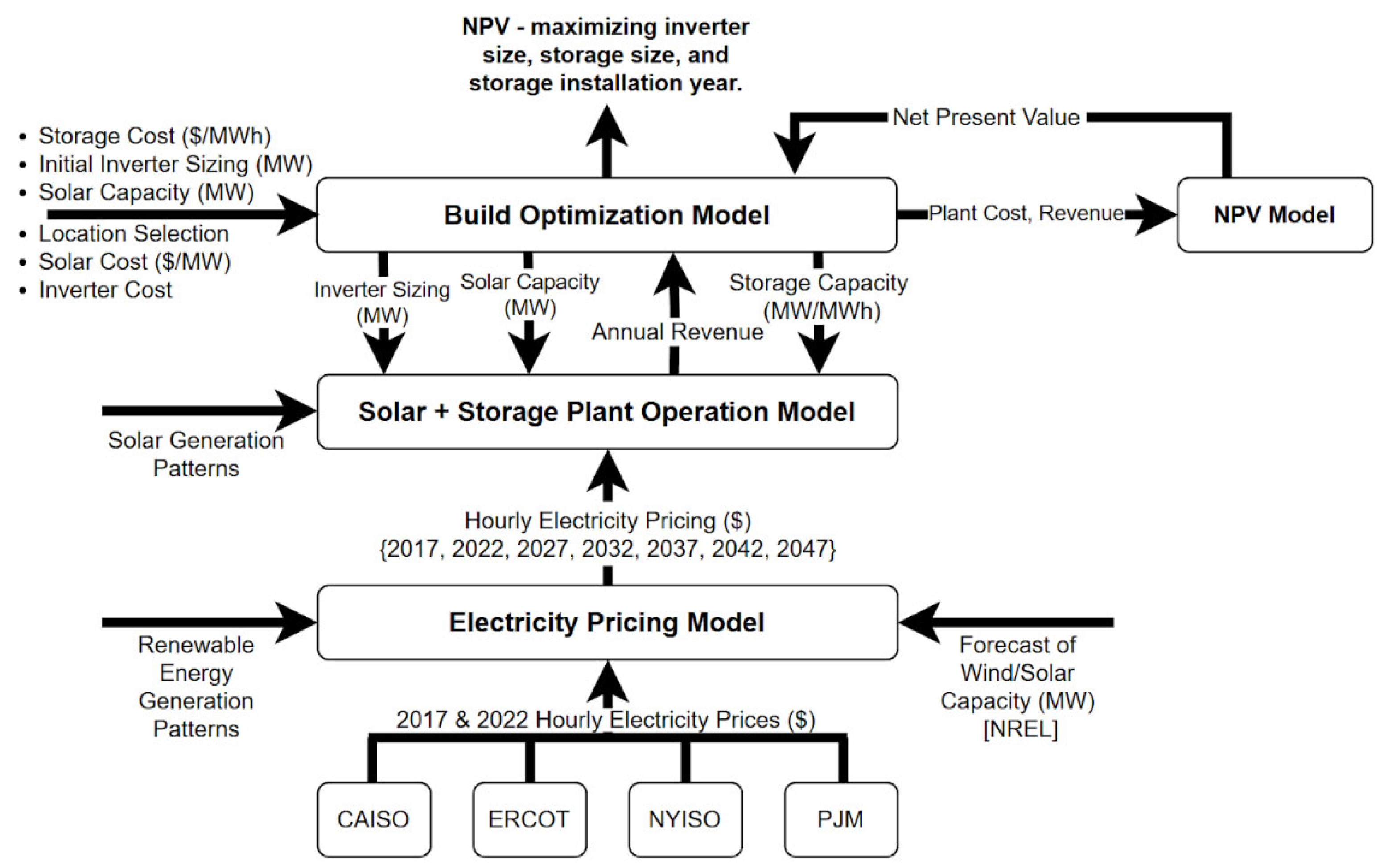
Figure 2.
Forced Storage Build-Year Analysis – CAISO: Showing optimal initial inverter capacity (MW, blue line), optimal storage capacity (MWh, red line), and NPV ($M, green bars). 2022 is the first operational year of the plant, and 2047 is the final projected operational year of the plant. The solar-only scenario represents the plant operation with storage constrained to zero. Optimal storage and inverter capacity tend to increase if storage is added in later years, due to the lower capital cost of storage. However, the overall NPV maximum is in 2032, a balance between the falling costs of storage and the opportunity cost of waiting to add storage.
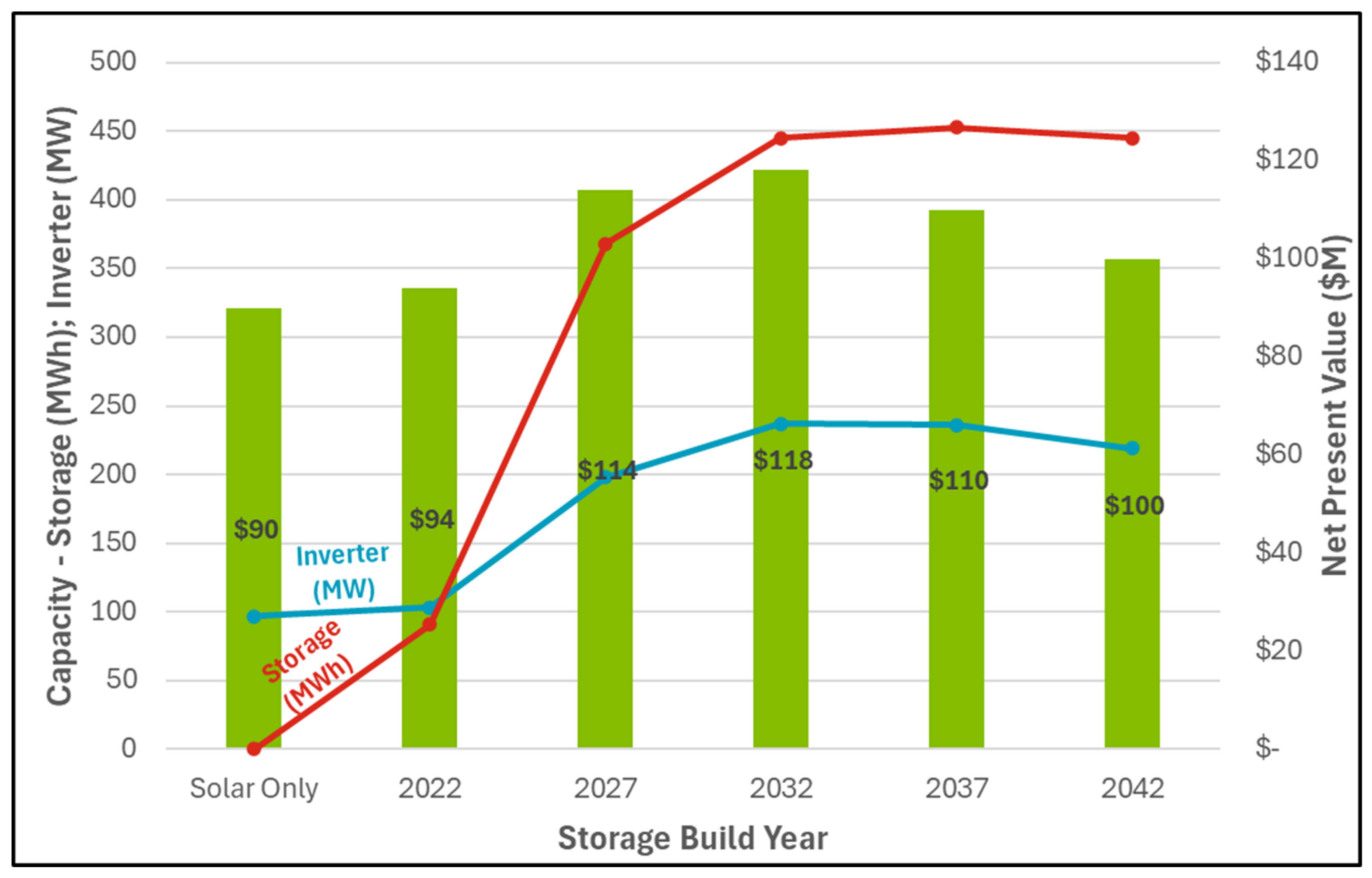
Figure 3.
Forced Storage Build-Year Analysis – ERCOT: Showing optimal inverter capacity (MW, blue line), optimal storage capacity (MWh, red line), and NPV ($M, green bars). 2022 is the first operational year of the plant, and 2047 is the final projected operational year of the plant. The solar-only scenario represents the plant operation with storage constrained to zero. Optimal storage and inverter capacity is much higher in ERCOT than in other locations, due to the inherent profitability of storage.
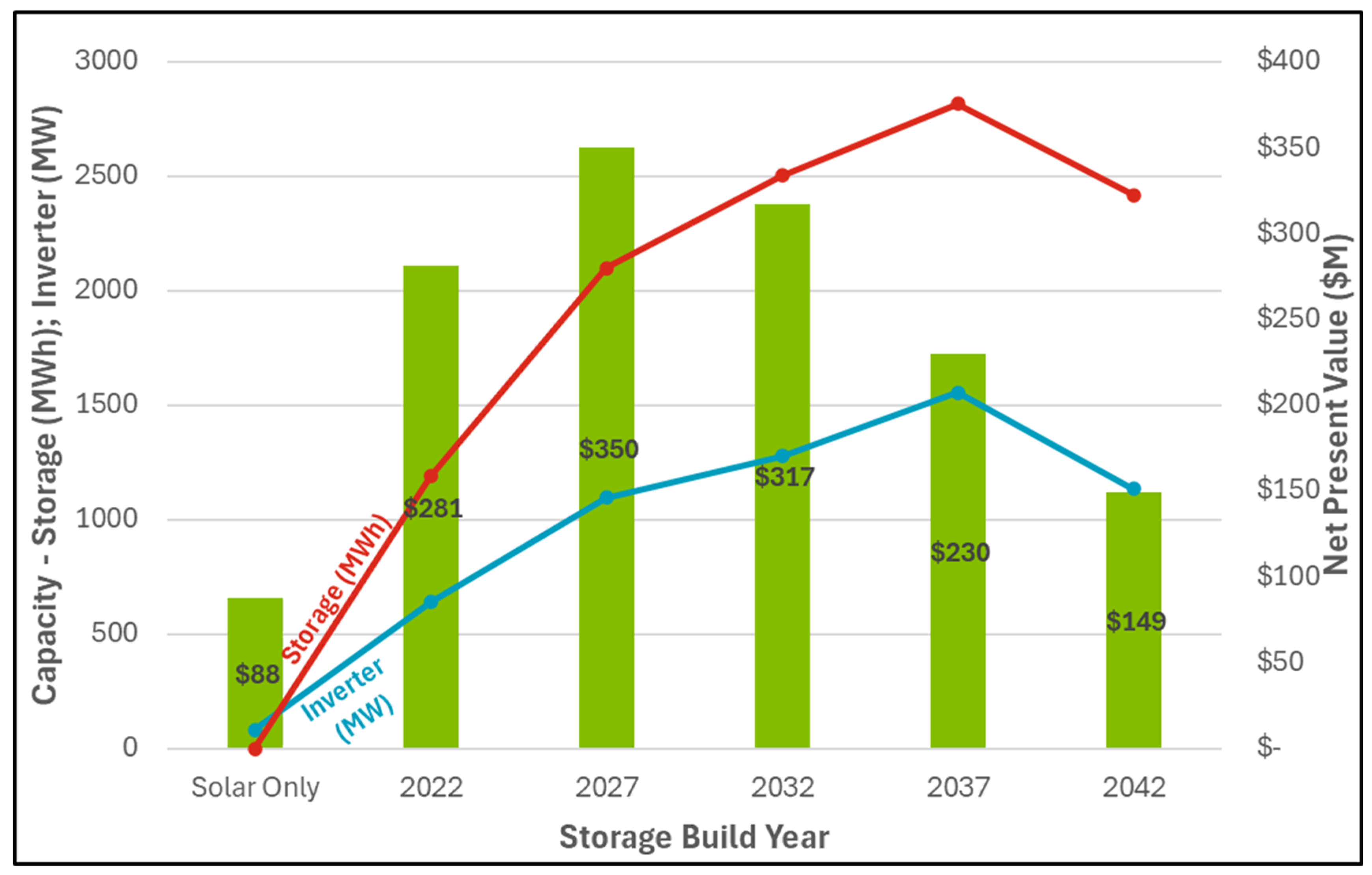
Figure 4.
Forced Storage Build-Year Analysis – NYISO: Showing optimal inverter capacity (MW, blue line), optimal storage capacity (MWh, red line), and NPV ($M, green bars). 2022 is the first operational year of the plant, and 2047 is the final projected operational year of the plant. The solar-only scenario represents the plant operation with storage constrained to zero. If storage is constrained to be built in 2022, the model chooses zero storage and reproduces the solar-only results.
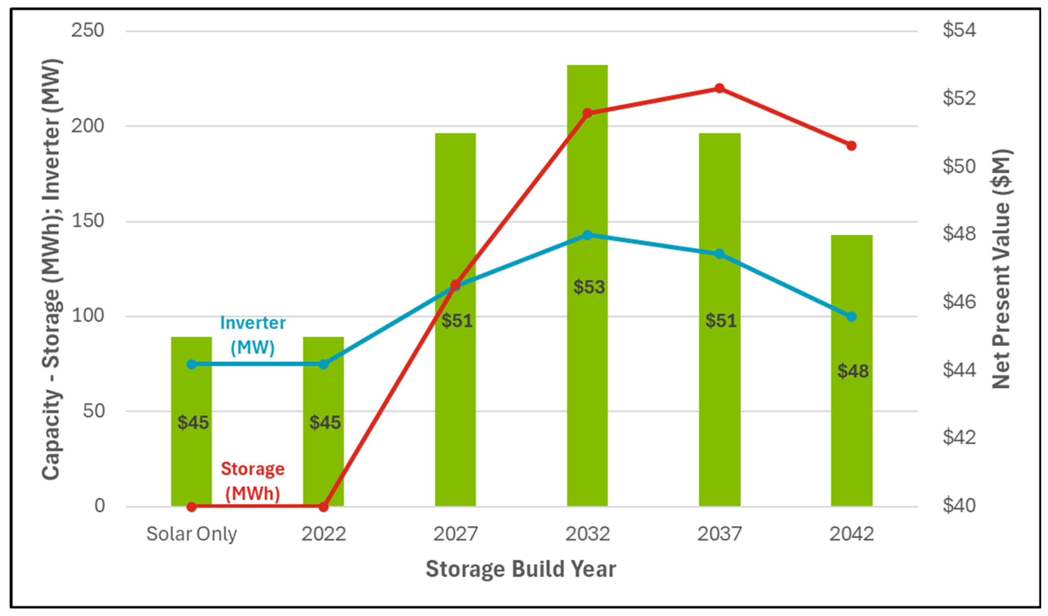
Figure 5.
Forced Storage Build-Year Analysis – PJM: Showing optimal inverter capacity (MW, blue line), optimal storage capacity (MWh, red line), and NPV ($M, green bars). 2022 is the first operational year of the plant, and 2047 is the final projected operational year of the plant. The solar-only scenario represents the plant operation with storage constrained to zero. If storage is constrained to be built in 2022, the model chooses zero storage and reproduces the solar-only results.
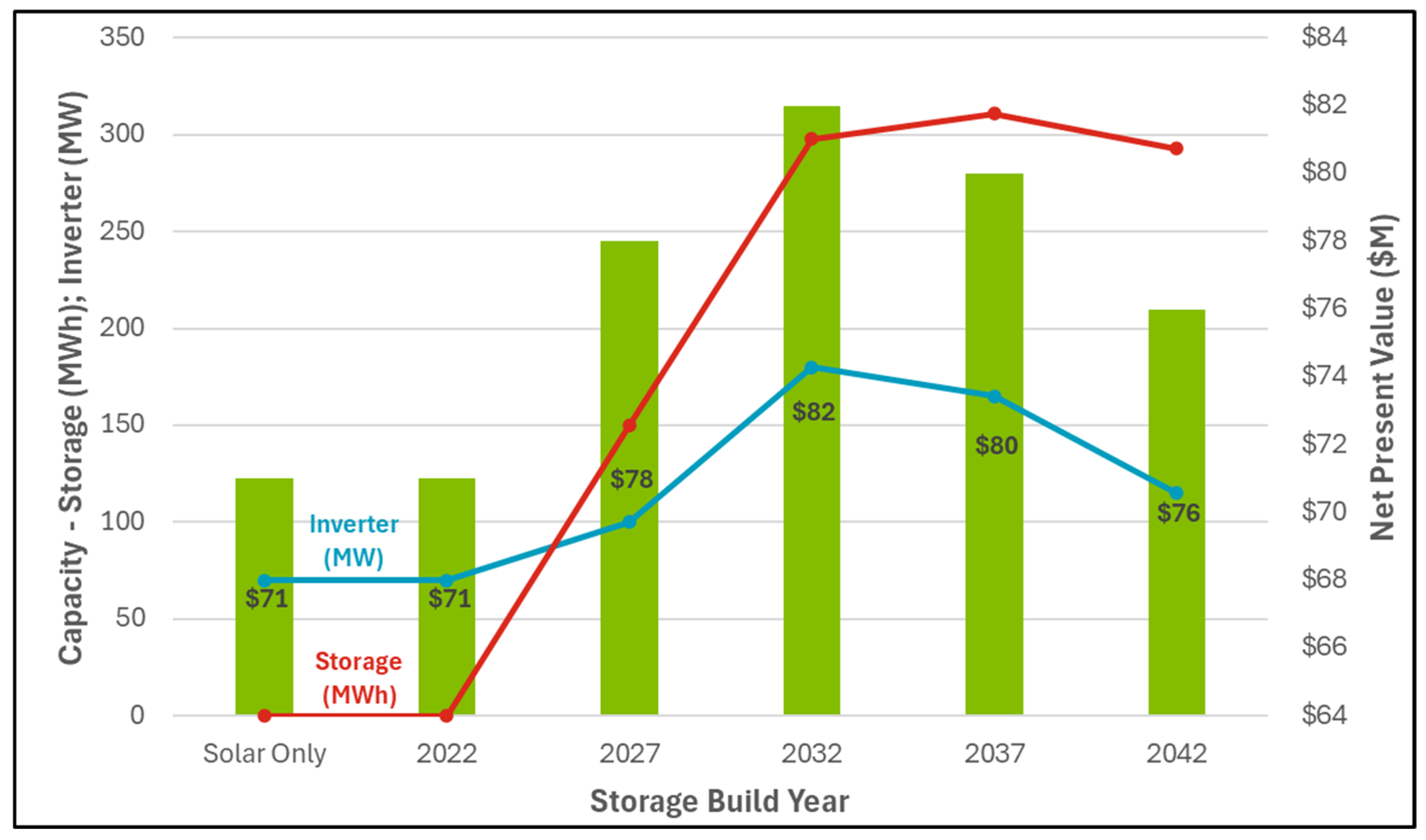
Figure 6.
Effect of 30% Subsidy on storage – CAISO: Three tested conditions: no subsidy (green), a temporary 30% subsidy that expires in 2023 (red), and a fixed 30% subsidy that stays through the entire operational period (red). 5601, 8434, and 8073 build scenarios were simulated, respectively. A: Net present value in millions of the build scenarios in CAISO by storage build year. B: Optimal storage capacity in CAISO by storage build year in MWh.
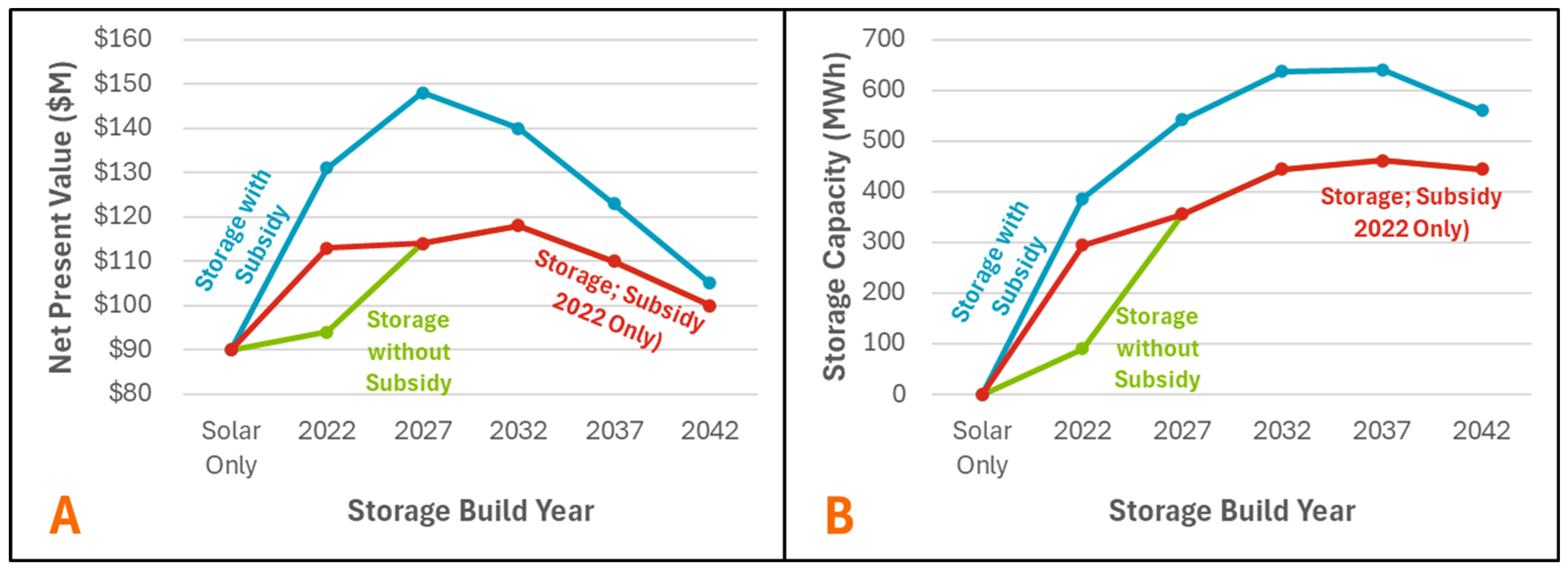
Figure 7.
Effect of Future Battery Pricing on Storage Capacity in ERCOT: Optimal storage capacity under base case conditions (in MWh, shown in green) for battery prices, low-cost conditions (in MWh, shown in blue), and high-cost conditions (in MWh, shown in red). 2022 is the first operational year of the plant, and 2047 is the final projected operational year of the plant. All scenarios run with standard conditions (see table 2) except for future battery pricing. Each storage build year contains the optimal conditions for a single plant (i.e., one build scenario), not the progression of the plant over time.
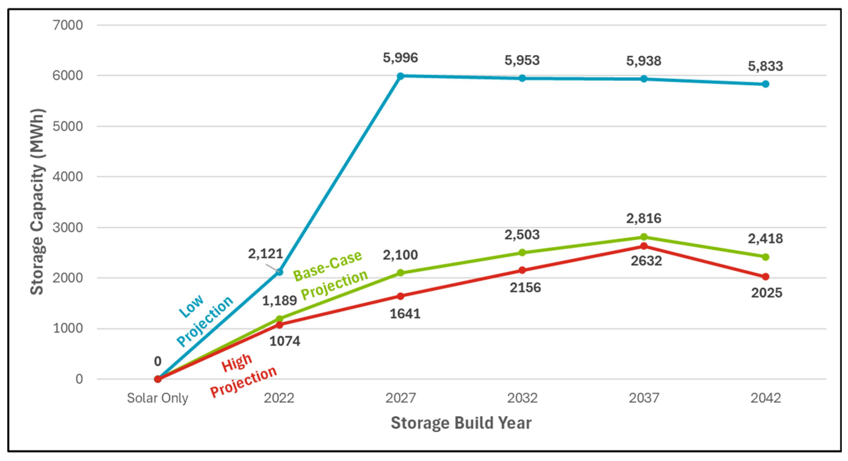
Figure 8.
Battery Charge/Discharge Rate Sensitivity Analysis: Sensitivity analysis in CAISO of battery duration type on: A) Projected future BESS prices from NREL Storage Futures Study [27], B) optimal build NPV ($M), C) optimal inverter capacity (MW), D) and optimal storage capacity (MWh). Battery types include 2-hour (purple), 4-hour (orange), 6-hour (green) and 8-hour (blue) charge/discharge rates. The number of hours corresponds to the time required for the battery to fully charge or discharge, with lower numbers corresponding to faster but more expensive batteries. The model was run until no improvements on NPV were observed for consecutive generations (average: 6831 scenarios).
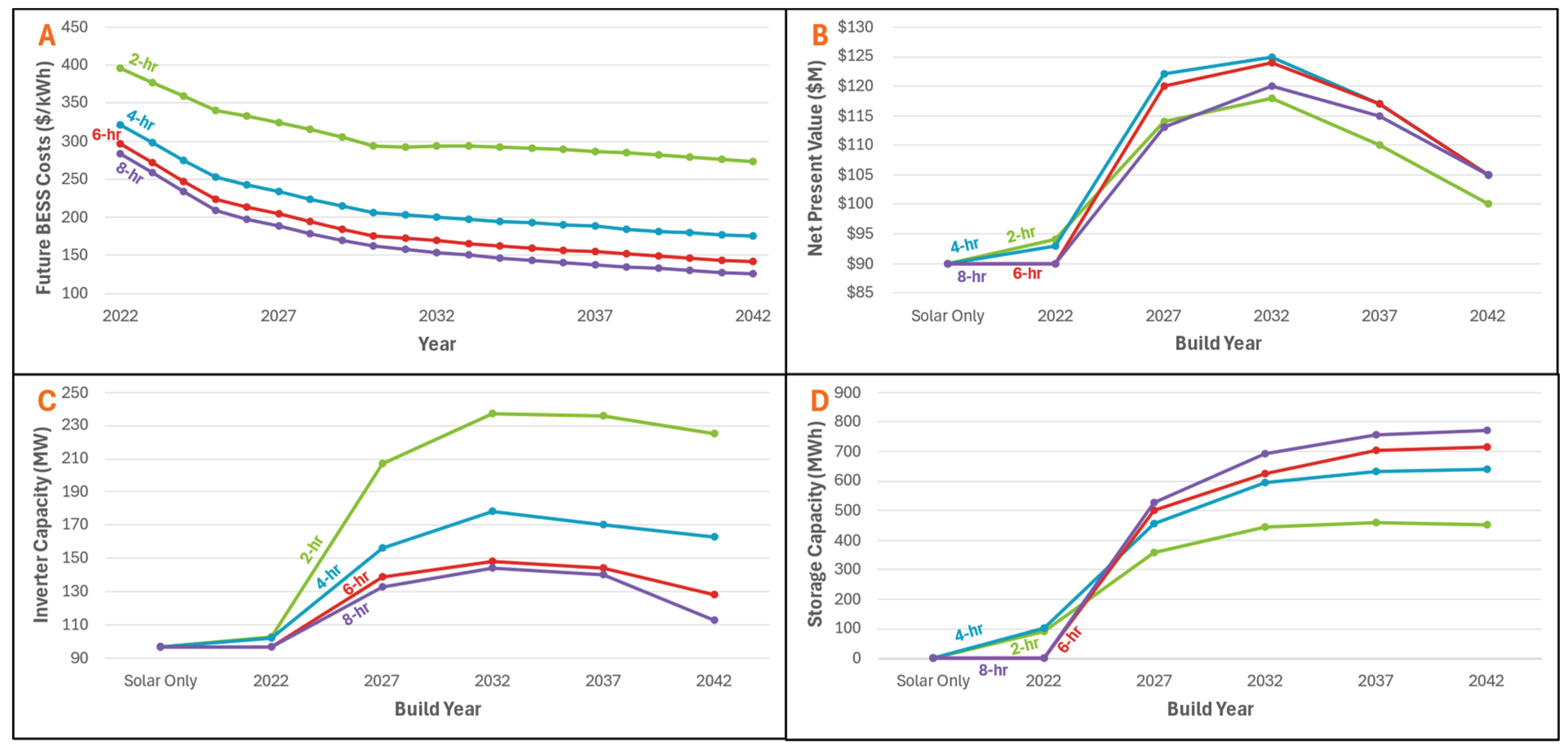

Table 1.
Optimization Parameters used in the high-level optimization.
| Optimization Parameter | Parameter Definition |
| Utility-Scale Solar | 100 MW Fixed Axis Solar |
| Storage Capacity | [0-600] MWh (NY, CA, PJM) [0-6,000] MWh (TX) |
| Inverter capacity | [0-400] MWh (NY, CA, PJM) [0-4,000] MWh (TX) |
| Storage Addition Years | 2022, 2027, 2032, 2037, 2042 |
| Solar + Inverter Capital Costs, Operation, & Maintenance | Paid as a fixed rate loan over the plant operation period. |
| Battery Costs | Paid over a 15-year battery lifespan – estimated.1 |
1New loan rate is calculated at the end of battery life.
Table 2.
Optimal Build Results – Base Case.
| Region | Optimal Conditions | ||||
| Plant NPV | Inverter Capacity (MW) | Storage Capacity (MWh) | Storage Build Year | Number of Cond. Simulated | |
| CAISO | $118M | 237 | 445 | 2032 | 1271 |
| ERCOT | $350M | 1,094 | 2,100 | 2027 | 970 |
| NYISO | $53M | 143 | 207 | 2032 | 1095 |
| PJM | $82M | 180 | 298 | 2032 | 1296 |
Disclaimer/Publisher’s Note: The statements, opinions and data contained in all publications are solely those of the individual author(s) and contributor(s) and not of MDPI and/or the editor(s). MDPI and/or the editor(s) disclaim responsibility for any injury to people or property resulting from any ideas, methods, instructions or products referred to in the content. |
© 2025 by the authors. Licensee MDPI, Basel, Switzerland. This article is an open access article distributed under the terms and conditions of the Creative Commons Attribution (CC BY) license (http://creativecommons.org/licenses/by/4.0/).
Copyright: This open access article is published under a Creative Commons CC BY 4.0 license, which permit the free download, distribution, and reuse, provided that the author and preprint are cited in any reuse.


