
Submitted:
20 May 2025
Posted:
20 May 2025
You are already at the latest version
Abstract
Optimizing networks under large-scale, multidimensional, and dynamic demand presents a significant challenge. This complexity is further amplified when solving network-based Uncapacitated Facility Location Problems (UFLP), which are well-known for their NP-hardness. Current large-scale analytical approaches, such as Neighborhood Search (NS) and Variable Neighborhood Search (VNS), face limitations in either solution quality or computational efficiency, predominantly due to their reliance on either unstable Random Initialization (RI) or computationally expensive Greedy Initialization (GI). Considering demand intensity and network topology, this research proposes the Demand-Weighted Roulette Wheel Initialization (DWRWI) strategy. This novel initialization method strategically prioritizes high-demand and centrally located network nodes, thereby creating high-potential initial facility configurations for improvement algorithms. Scenario-based testing demonstrates several distinctive strengths of DWRWI: Compared to RI and GI, DWRWI better identifies high-demand, central network nodes, yielding superior initial solutions early in optimization. For example, in the large-scale network, DWRWI-initialized NS achieved a higher Silhouette score (0.3859) than RI (0.3833) and GI (0.3752). Additionally, DWRWI reduces computation time by about 28% compared to Greedy-initialized NS while maintaining competitive costs. By integrating demand-weighted distance and stochastic optimization theory, DWRWI significantly reduces computation time while ensures more uniform customer-to-facility assignments aligned closely with spatial demand distributions.
Keywords:
stochastic optimization
; heuristic algorithm
; network-based Uncapacitated Facility Location Problem
; Demand-Weighted Roulette Wheel Initialization
; demand intensity
; network topology
1. Introduction
Facility-location problems constitute a cornerstone of operational research, seeking optimal placement of candidate sites to curb transportation and facility costs while sustaining high service efficiency. Their relevance permeates logistics, supply-chain design, and urban planning, where strategic choices must weigh distance, time, capacity, and the comparative expenses of building versus leasing warehouses. Given the multitude of potential demand nodes and the problem's inherent complexity, mathematical models and advanced algorithms have become indispensable, driving extensive academic inquiry and delivering data-driven guidance for real-world decision-makers [1,2,3]. The p-median problem (pMP) and its derivative, the uncapacitated facility location problem (UFLP), exemplify Discrete Location Problems (DLP) concerned with choosing facility sites from finite candidates to minimize service costs [3]. The study of DLP has its roots in several key milestones. Originating with Weber's planar warehouse model [4] , formal network treatment emerged when Hakimi [5] defined the pMP, sparking systematic research into optimal facility placement and customer assignment. Tansel’s 1983 survey refined this field by classifying network variants and outlining efficient solution techniques [6]. In the same year, Krarup and Pruzan incorporated fixed and variable cost elements, transforming the pMP into what is now recognized as the UFLP. Subsequent scholarship has broadened UFLP applications—from uncapacitated warehouse siting [7] to urban service deployment [8]—solidifying these models as foundational tools in contemporary location analysis.
In 1979, Kariv and Hakimi proved that the pMP is NP-hard [9], indicating its computational complexity. This result highlighted the difficulty of solving general instances of the problem on arbitrary networks. Therefore, pMP and UFLP are recognized as generalized mathematical problems that have been extensively studied in recent years through the lens of optimization theory. The primary problem has motivated significant methodological advancements across exact, heuristic, and metaheuristic approaches. Traditional exact algorithms remain indispensable for small-to-medium scale instances (<1,000 nodes) due to their rigorous optimality guarantees. Enhanced branch-and-bound techniques [10,11,12] and decomposition methods—particularly Lagrangian relaxation [13,14,15] and Benders decomposition [16,17]—have demonstrated success in decoupling facility selection from customer allocation decisions. Heuristic approaches address scalability limitations through computationally efficient strategies. GPU-accelerated parallel vertex substitution algorithms achieve linear time complexity for large-scale networks [18], while classical interchange heuristics [19] and greedy algorithms [20,21] provide rapid feasible solutions. Atta et al. [22] report that these methods maintain computational efficiency within ±15% optimality thresholds for ORLib benchmarks, though they risk local optimum entrapment through path dependency—a limitation requiring 23% additional iterations on average to mitigate [23]. Metaheuristics excel in handling complex UFLP variants through global exploration capabilities. Genetic algorithms [24,25,26,27] and hybrid evolutionary learning frameworks [28] outperform deterministic methods by 13% in non-convex fixed-cost scenarios through multi-modal optimization. Recent advancements like discrete evolutionary algorithms [29] demonstrate accelerated convergence rates while maintaining solution quality. Despite these strengths, parameter sensitivity in population-based methods (e.g., particle swarm optimization [30]) and memory-intensive operations in tabu search [31] present implementation challenges for resource-constrained environments.
For pMP-type problems, increasing data scale, customer counts, and the expansion of potential facility locations considerably complicate the solutions. Conventional exact methods like the branch-and-bound algorithm have high exponential increases in computational time and complexity as problem size grows [23]. Meanwhile, heuristic methods, like genetic algorithms, are prone to entrapment in local optima [32]. However, in real-world applications, location problems tend to appear in the form of more complex networks, such as express logistics companies needing real-time responses for daily distribution hub strategies, typically manifest as extremely large-scale and complex networks involving substantial numbers of demand points and network nodes, further complicating solution methods. In response, recent advancements in Neighborhood Search (NS) and Variable Neighborhood Search (VNS) have facilitated progress in addressing these challenges. The classic NS [33] systematically reassigns facility-customer pairs within predefined spatial clusters. While it achieves local optimality, it suffers from limited global search capabilities due to its myopic exploration. The latest VNS [34] improves upon the earlier NS method by incorporating the interchange technique into an iterative structure that involves shaking, local search, and evaluating swaps. This approach has been demonstrated to perform effectively in large-scale cases. Subsequently, Ghosh [23] refined the local search phase of the VNS method. Amrani et al. [35] proposed a hybrid heuristic combining VNS with tabu search to optimize multi-product production-distribution network design problems involving alternative facility configurations and concave inventory costs. Their framework was tested on cases ranging from 500 to 1,000 demand areas and 60 to 100 potential distribution centers. Hansen et al. [36] introduced a primal–dual VNS, which leverages dynamic neighborhood structure adjustments and heuristic optimization techniques to enhance algorithmic efficiency and scalability. Irawan & Salhi [37] proposed a novel approach integrating demand point aggregation with multi-stage optimization to tackle large-scale p-median problems. Their method combines mini-VNS with full VNS to improve both solution efficiency and quality. Herrán et al. [38] further enhanced the efficiency of VNS for the Hamiltonian p-Median Problem (HpMP) by 22%, leveraging problem-specific neighborhood structures that balance cluster density and spatial dispersion. Modern variants, such as the RL-driven VNS by Croci et al. [39], integrate reinforcement learning to optimize neighborhood-switching thresholds, thereby mitigating the traditional need for manual parameter calibration.
Although the above literature has extensively explored NS and VNS methodologies for solving pMP and UFLP problems, several research gaps persist. First, while substantial progress has been made in applying VNS solutions to pMP and its numerous variants, such as the Hamiltonian p-Median Problem (HpMP) [38], the α-neighbor p-Median Problem [40], the balanced p-Median Problem [39] and the Capacitated p-Median Problem (CpMP)—there remains a lack of clear distinction and definition between discrete and Network-based UFLP problems. This gap limits the development of solutions and model definitions for pMP variants of Network-based UFLP problems. Second, both NS and VNS algorithms rely heavily on predefined spatial clusters, with initialization methods significantly influencing the quality of subsequent iterative improvements. Commonly referred to as constructive methods (as opposed to NS and VNS, which are considered improvement techniques), the prevailing initialization method—Greedy algorithms [20,21]—has been demonstrated through this study to be highly limited in large-scale scenarios. Nonetheless, most existing literature continues to focus on refining VNS algorithms while the exploration of initialization methods remains insufficient [17,36,37]. Third, there is a lack of multi-level performance tests and comparative analyses across varying scales of data for NS and VNS methods. For instance, the VNS tests conducted by Amrani [35] on network-based CFLP problems are notably limited in data scale and case diversity. Similarly, the four methods evaluated in Gwalani, Tiwari, & Mikler [41]—Alternate Selection and Allocation Algorithm, Exchange Algorithm, Global/Regional Interchange Algorithm, and Greedy Addition/Myopic Algorithm—are relatively outdated.
To address the complexities inherent in large-scale network-based UFLP, this research aims to innovate the existing initialization methods, which can promote the effectiveness of both the NS and VNS. Based on a mathematical formulation that incorporates user requests and network topology traits explicitly, the study positions NS and VNS within a systematic comparison against a spectrum of solution approaches, including exact algorithms, heuristics, metaheuristics, and relaxation techniques. Special emphasis is placed on the development and theoretical justification of a novel demand-weighted roulette wheel initialization method, which leverages user demand and network structure to enhance both solution quality and computational efficiency. This innovative approach is analytically demonstrated to outperform conventional greedy strategies in terms of algorithmic complexity and practical effectiveness, particularly within NS and VNS frameworks. A comprehensive empirical evaluation is undertaken using a variety of datasets, spanning from small-scale synthetic instances to real-world transportation networks across six cities. The testing methodology encompasses three core dimensions: multi-case comparative analysis, repeated trials for robustness assessment, and cross-method benchmarking, facilitating a thorough evaluation of solution quality, stability, and generalizability. Through these contributions, the study not only proposes methodological enhancements but also bridges theoretical and practical advancements for network-based UFLP, offering insights of broad relevance for the optimization community.
The structure of this paper is organized as follows: Chapter 2 introduces the formal definition of the Network-Based Uncapacitated Facility Location Problem (N-UFLP). Chapter 3 presents the methodological framework, with particular emphasis on the proposed Demand-Weighted Roulette Wheel Initialization (DWRWI) and its integration into enhanced metaheuristic algorithms NS2025 and VNS2025. Chapter 4 presents a comprehensive empirical evaluation across multiple real-world scenarios, including small-scale, large-scale, and ultra-large-scale networks, to assess the performance of the proposed methods in comparison to state-of-the-art benchmarks. Chapter 5 synthesizes the theoretical and experimental findings to critically discuss the strengths, limitations, and practical implications of DWRWI-based methods. Finally, Chapter 6 concludes the paper by summarizing the contributions, outlining the methodological innovations, and identifying promising directions for future research.
2. Problem Definition
2.1. Network-Based Uncapacitated Facility Location Problem (N-UFLP)
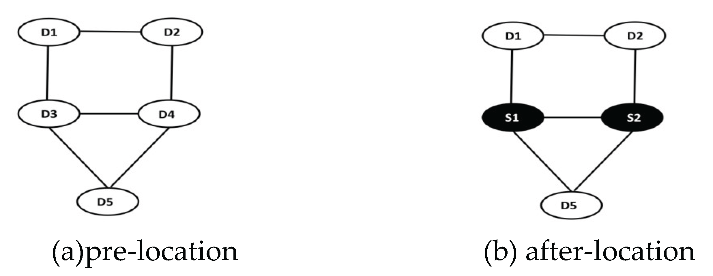
The Uncapacitated Facility Location Problem (UFLP), also known as the Simple Facility Location Problem (SFLP), traditionally involves selecting optimal facility locations from a set of discrete candidate points to serve spatially distributed customer zones. Generally speaking, UFLP minimizes total system cost by deciding which candidate sites to open—hence the number and locations of facilities—while explicitly accounting for customer locations, customer demand, transportation costs, and facility setup costs. While prior studies [35] have addressed UFLP scenarios, the network-based problem lacks a rigorous definition. This study formalizes the Network-based Uncapacitated Facility Location Problem (N-UFLP) by contrasting it with classical discrete UFLP and specifying its defining characteristics:
- Node Location Integration: Facilities and customers are co-located within a unified node set, where the first N nodes serve dual roles as both customers and candidate facility locations. This contrasts with traditional UFLP, which treats facilities and customers as distinct sets and introduces self-service constraints (e.g., a facility can serve itself). This approach better reflects practical applications such as telecommunications, logistics, and waste management systems, where real-world nodes (e.g., intersections, hubs, or urban locations) can act both as service origins and destinations, improving model fidelity to network realities [5,42,43].
- Path-Dependent Distance Metric: Transportation costs are determined by shortest-path distances on the network, calculated as the sum of edge weights between nodes using the Floyd-Warshall algorithm. Unlike classical UFLP models, which assume Euclidean distances or direct transportation costs, this approach dynamically computes path costs based on the network topology. For many network applications, e.g., transportation and waste collection, using shortest-path network distances instead of geometric distances is essential for operational feasibility, as real-world routes are dictated by the topology of the network and its connectivity [2,43,44].
- Network Distance Matrix: A precomputed M×M matrix stores all-pairs shortest path distances for M nodes, replacing conventional transportation cost matrices. Storing precomputed shortest-path distances allows large-scale problems to be solved more efficiently, enabling rapid cost evaluations within metaheuristic or exact optimization frameworks commonly used in both academic study and industrial practice [2,29].
- Network Connectivity Constraints: Accommodates disconnected subnetworks (e.g., isolated traffic zones) by introducing virtual edges to connect orphaned nodes to the nearest network component, ensuring full service coverage. This is especially vital in urban logistics, telecommunications, or emergency services, where service continuity across potentially disconnected or dynamically changing networks must be ensured [42,45]. Virtual or auxiliary links are routinely adopted in real-world applications to guarantee full coverage.
- Demand-Weighted Travelled Cost: Combines customer demand volumes with path distances to generate a demand-weighted travelled cost metric. Weighting travel costs by demand mirrors operational objectives in logistics, emergency services, and supply chain management, where both the volume and the distance traveled significantly influence the optimal facility placement and overall system efficiency [42,46].
Figure 1.
Network-based Uncapacitated Facility Location Problem.
These considerations lead to the inclusion of further constraints, reflecting realistic network structures and distance calculations that depend on actual travel paths rather than simple geometric distances. They will, in turn, become unique assumptions. To further formulate this problem, we firstly define sets and indices:
Nodes/Facilities: Let I={1,2,...,M}be the set of all nodes (with |I|=M), every node is a candidate for locating a facility.
Customers: Define the customer node/demand site subset as J⊆I, J={1,2,...,N} (N≤M) indicating that the first N nodes serve as customers and also as candidate facility locations (thus allowing co-location).acilities and customers) and j∈J refer specifically for customers.
Then, we define network structure
Adjacency-Based Distance Matrix (Dadj).
Define the adjacency-based distance between node
Indices: Let i, r∈I denote Index for nodes (both fi and node r as diradj. The matrix Dadj=[diradj]M×M is then specified by:
Let geodist (i,r) denote the Euclidean distance between nodes i and r, computed from their geographic coordinates given in the M×2 matrix nodeCoords when a node j with customer demand is identified as isolated (i.e., dij=∞ for all j∈J). The geodist function trigger condition occurs when either node i or r represents an isolated node with customer demand. This indicates that these nodes are special cases within the network data, often corresponding to unique subareas in real-world transportation networks or OD points connected via feeder branches. To ensure effective routing for demand originating from these isolated nodes, we connect them “virtually” to their geographically nearest reachable node kgeo via the Euclidean distance.
Shortest-path distance matrix (D)
The effective transportation distance used in the objective function is given by the matrix D=[dir]M×M, where each element is defined by:
where the shortest-path distance matrix D is calculated by Dadj through shortest-path algorithm. It is noteworthy that we employ path distance or demand-weighted traveled distance, rather than traditional adjacency-based distance metrics.
Finally, in the aspects of demand and cost, we define
Trip attraction (hj): Let hj represent the N×1 demand/trip attraction at customer node/demand site j.
- (a)
- Transportation Cost Rate (α): A scalar parameter α multiplies the effective distance to yield the transportation cost.
- (b)
- Facility Setup Cost (β): A scalar parameter β denotes the unitary fixed cost for opening a facility. This cost is assumed to be identical for all candidate locations.
- (c)
- Demand-weighted traveled distance (Wij): The transportation cost incurred when assigning customer demand hj to a facility at node i is given by Wij= hj · dij.
In N-UFLP, similar to the general types, we aim to minimize total costs by optimizing both facility locations and assignment relationships.
The conventional UFLP seeks to determine optimal facility locations under constraints such as ensuring all demand points are satisfied, establishing correspondence between facility assignments and demands, and often limiting the number of facilities due to resource constraints. In contrast, the N-UFLP introduces additional constraints by incorporating specific assumptions, including Node Location Integration and path-dependent distance metrics:
- Self-Service Feasibility:
- Path Consistency (Triangle-Inequality) Constraint:
- Variables xij and yi are the decision variables representing the assignment relationships and facility location, respectively
2.2. Notations
| Symbol | Definition |
| Sets | |
| I | Set of all nodes (∣I∣=M), including facilities and customers. |
| J | Subset of customer nodes/demand site (∣J∣=N), also candidate facilities. |
| S | Final set of selected facilities. S={s1,s2,…,sp}. p×1 Vector of indices. Output. |
| Asgmt. | 1×N Vector mapping customers to assigned facilities. Output. |
| K | Set of all candidate facility locations. K={1,2,...,N}. |
| Indices | |
| i, r ∈I | Indices for general nodes (facilities or customers). |
| j∈J | Index specifically for customer nodes. |
| t | Iteration index for facility selection, t=1,2,...,p,where p≤N. |
| k∈K | k∈K corresponds to a potential facility. |
| Parameters | |
| diradj | Adjacency-based distance between nodes i and r (direct edge length). |
| Dadj | M×M adjacency distance matrix. |
| dir | Shortest-path distance between nodes i and r. |
| D | M×M shortest-path distance matrix. |
| (hj)j∈J | Demand weight (trip attraction) at customer j (N×1 vector). Input. |
| Wij | Demand-weighted traveled distance from node i to node j. |
| α | Uniform facility setup cost. Input components. |
| β | Transportation cost rate per unit-distance-demand. Input. |
| p | Maximum allowed facilities. |
| Z(s) | TotalCost. Scalar objective value of solution S. Output. |
| Decision Variables | |
| yi | yi∈{0,1}: 1 if a facility is opened at node i; 0 otherwise. |
| xij | xij∈{0,1}: 1 if customer j is assigned to facility i; 0 otherwise. |
| Key Matrices | |
| NodeNames | M×1 cell array of unique node identifiers. Input components#. |
| NodeCoords | M×2 matrix of geographic coordinates (longitude, latitude). Input. |
| DistTable | L×3 matrix of adjacency distances (origin, destination, edge length). Input. |
| DistanceMatrix | M ×M matrix of precomputed shortest-path distances. Input. |
2.3. Assumptions
The N-UFLP proposed relies on the following assumptions:
- A customer node can be served by a facility co-located at the same node.
- All facilities incur identical fixed setup costs, i.e., no site-dependent cost variations.
- Facilities are either fully open or closed; partial opening is prohibited.
- Each customer is entirely served by a single facility.
- There is no upper limit on the demand a facility can serve.
- All costs, demands, and distances are deterministic and known with certainty.
- The maximum number of facilities p is the square root of N (budget-constrained).
3. Methodology
3.1. Baseline Methods
This section presents the overarching methodological framework utilized in this study. Neighborhood Search (NS) and Variable Neighborhood Search (VNS) algorithms are widely recognized as effective improvement algorithms for solving large-scale Network-based Uncapacitated Facility Location Problem (N-UFLP); however, their performance is significantly influenced by the quality of constructive algorithm, which are typically generated via randomized, roulette wheel, or greedy initialization approaches. Despite their prevalence, these construction methods demonstrate notable limitations when applied to large-scale N-UFLP instances. Therefore, this section first explores, from a theoretical perspective, strategies to refine these initialization algorithms, aiming to overcome their inherent shortcomings. Furthermore, we integrate these enhanced methods with NS and VNS to enhance the overall efficiency and capability in solving N-UFLP problems.
3.1.1. Roulette Wheel Initialization (RWI)
Roulette Wheel Initialization, as described by Celebi [46], is widely adopted as a heuristic approach, most notably for enhancing iterative selection mechanisms in genetic algorithms and the initialization process of K-Means++. The essence of this method lies in its probabilistic selection scheme: at iteration t, the probability of selecting node k from the remaining candidates K\St-1 is proportional to its weight wk, normalized over all unselected nodes. Formally:
Where:
- St-1 is the set of facilities already selected before iteration t.
- K\St-1 is the set of remaining candidate nodes.
- In the basic version one may set wk=(dkadj)min.
- st~Discrete(P(·)) denotes that st is drawn from the discrete distribution defined by the probabilities Pk.
This ensures that nodes with higher weights have a correspondingly greater chance of being selected, thereby guiding the initialization process in a data-driven manner.
3.1.2. Greedy Initialization (GI)
The greedy heuristic initialization method, widely used in facility location problems (Celebi et al., 2013), iteratively selects facilities to directly minimize the total cost defined in the N-UFLP objective function. This method prioritizes immediate cost reduction but often lacks exploration diversity, potentially trapping solutions in local optima. Let:
- St - denote the set of selected facilities after iteration t (S0=∅).
- let K\St-1 be the candidate nodes, unselected candidate nodes (recall K={1,2,...,N}).
Phase 1 (Initial Facility Selection)
Intialize S0=∅, t=0, K\St-1=K.
Phase 2 (Iterative Marginal-cost evaluation)
While |St|<p, set t=t+1:
Cost Evaluation
For each candidate node k∈K\St-1, compute the temporary total cost Z(St-1 ∪ {k}) incurred by opening k:
Fixed Facility Cost:
Total Cost:
- (a)
- Selection Criterion
Select the candidate k*∈K that maximizes the marginal cost reduction:
- (b) Update
Add k* to the facility set and remove it from candidates:
3.1.3. Neighborhood Search Algorithm (NS) and Greedy-initialized Neighborhood Search
Neighborhood Search (NS) and Variable Neighborhood Search (VNS) are often adopted as improvement methods. Specifically, Neighborhood Search (NS), proposed by Maranzana [33], seeks to minimize total costs, aligning with the objective of the N-UFLP baseline. The general procedure of NS involves iteratively exploring neighboring solutions to identify cost reductions:
Phase 1 (Initialization)
Generate S via Greedy Initialization or other initialization methods.
Phase 2 (Neighborhood Structure)
Define operators for search:
(2a) For each iteration, alternately reassigns all customers to their nearest open facility.
(2b) For each facility, seek the optimal new location (from the M possibilities) that minimizes the total demand-weighted distance to its assigned customers.
Phase 3 (Iterative Improvement)
(3a) Evaluate all neighbors of S.
(3b) Accept the neighbor S′ with the lowest total cost Z(S′).
(3c) Repeat until no further improvement occurs.
Given an initial facility set S(|S|=p), each NS iteration involves: Evaluating all possible swaps between i∈S and k∈K\S, giving approximately p×(M-p)≈pM neighborhood solutions. For each neighbor, all customers are reassigned to their nearest open facility, requiring N operations. Thus, each iteration of NS has complexity O(p·M·N). For common swap/add/drop implementations, this is often simplified to O(p2N) as seen in the baseline. If NS executes for T total iterations, the overall complexity Greedy-initialized NS is:
3.1.4. Variable Neighborhood Search (VNS) and Greedy-initialized Variable Neighborhood Search
The Variable Neighborhood Search (VNS) [34] extends NS by introducing dynamic neighborhood structures to escape local optima and explore broader solution spaces. The general procedure is as follows:
Phase 1 (Initialization)
Generate S via Greedy Initialization or other initialization methods.
Phase 2 (Multiple Neighborhoods)
Define N1, N2,...,Nk with increasing complexity:
- N1: Single-swap operator.
- N2: Double-swap operator.
- N3: Demand-weighted perturbation.
Phase 3 (Shaking)
Randomly perturb S within Ni to escape local optima.
Phase 4 (Local Search)
Apply NS to refine the perturbed solution.
Phase 5 (Neighborhood Switch)
If no improvement, transition to Ni+1.
The analysis of VNS complexity is structured into three distinct sections: VNS employs k distinct neighborhood structures; Within each neighborhood, a local search is carried out; each has complexity O(p2N); If the primary VNS process runs for L outer iterations, and within each the full suite of k neighborhood is explore. The total overall complexity of Greedy-initialized Variable VNS is
While Greedy-initialized NS and VNS frameworks are widely adopted for their conceptual simplicity and solution quality in small to moderate-sized problems, they suffer from significant limitations regarding computational complexity and speed, especially as network scale increases.
3.2. Demand-Weighted Roulette Wheel Initialization (DWRWI)
3.2.1. Theory
Traditional NS and VNS approaches often rely on predefined spatial clusters, which can lead to suboptimal facility placements, particularly in scenarios involving large-scale N-UFLP. Meanwhile, classical Roulette Wheel Selection (RWS) typically considers only the two-dimensional spatial positions and the Euclidean distances between nodes, making it unsuitable for the N-UFLP. Furthermore, Greedy Initialization significantly increases the computational complexity of both NS and VNS methods. To address these limitations, we propose a Demand-Weighted Roulette Wheel Initialization method, which integrates demand information and network topology with a probabilistic selection mechanism to generate more effective initial facility configurations. By replacing the conventional initialization with our method DWRWI, we aim to enhance the exploration capability and overall performance of NS/VNS algorithms in solving large-scale N-UFLP.
Let the following notation be established:
- t: Iteration index for facility selection, t=1,2,...,p,where p≤N.
- St={s1,s2,...,st}: Set of currently selected facility locations by the end of iteration t.
- st: Newly selected facility at the t-th iteration, where st∈K\St-1.
Phase 1 (Initial Facility Selection)
The first facility s1 is selected uniformly at random from the first N customer nodes K to avoid bias toward densely populated regions. This ensures spatial dispersion in the initial configuration.
(11)
Phase 2 (Iterative Roulette Wheel Selection)
For each subsequent iteration (t=2,....,p), one additional facility st is selected from the remaining candidates K\St-1, as follows:
- (a)
- Minimum Distance Calculation:
For each candidate node k∈K\St-1, calculate the shortest-path distance to the nearest already-selected facility:
(12)
- (b) Weight Assignment:
Assign a weight wk to node k proportional to its unsatisfied demand hk and minimum distance from existing facilities dkmin:
(13)
which improved over the original non-demand-driven Initialization method. In comparison, the Roulette Wheel Initialization used the mathematical expression wk=(dkadj)min, where the initialization of nodes was determined solely by their Euclidean distances. While this method offered simplicity, it failed to account for other critical factors that could influence optimal node placement in many real-world scenarios. In comparison, the proposed formula in this paper, wk is to balance two objectives:
- Demand Satisfaction: Prioritize nodes with higher demand (hk) to maximize service coverage.
- Spatial Dispersion: Favor Nodes farther from existing facilities (dk)minto avoid clustering while considering network topology.
Combining these terms multiplicatively ensures that both conditions must be satisfied for a node to receive high weight: Firstly, a high-demand node close to existing facilities (hk large, dkmin small) is less preferred than one with similar demand but greater distance. Then, a distant node with low demand (dkmin large, hk small) is also deprioritized. Candidates with both higher demand and greater distance from current facilities receive larger weights, encouraging coverage expansion and demand satisfaction.
- (a)
- Probability Normalization:
Normalize the weights to obtain selection probabilities:
(14)
Any node already selected (j∈St-1) is excluded (Pk=0). This equation represents normalization that converts absolute weights (wk) into selection probabilities (Pk) to:
- Ensure valid probability distribution (∑Pk=1)
- Proportionally allocate selection likelihood based on relative weights.
This aligns with RWS principles in stochastic optimization, where higher-weighted candidates have proportionally higher chances of selection.
(d) Roulette Wheel Selection
Generate a random number γ ~U(0,1) and select the next facility st such that:
(15)
Phase 3 (Termination criteria)
Iterative sampling stops when t=p, which means an upper bound on the number of facilities has been reached. If none of the above holds, set t←t+1 and return to Phase 2.
3.2.2. Theorem (Correctness and Termination)
Let K={1,2,...,N} be a finite set of candidate sites, each with a strictly positive demand hk>0 and finite shortest-path distances D(k,i) between all pairs. Let p be given facility number (1≤p≤N). Apply the four-step procedure below:
(i) Distance calculation
(ii) Weight assignment
(iii) Probability normalization
(iv) Roulette-wheel sampling
Repeat these steps, starting from an initial selection, and after each step, remove the selected site from the candidate list. Then, the following properties hold:
Theorem 1. Well-defined probabilities: At each iteration t (where 1≤t≤p), the probabilities vector
Proof of Theorem 1. Well-defined probabilities: At each iteration t, in the distance computation step (a), we caculate dkmin ≥ 0 for every unselected candidate k (i.e., for all k∈K\St-1). Because demands hk>0, the weights produced in step (b), wk(t)=dkmin·hk, are strictly positive. Therefore, the denominator in the normalization step (c), ∑k∈K\St-1wk(t) , is always positive. The resulting normalized probabilities Pk(t)=wk(t)/(∑wk’(t)) are strictly between 0 and 1, and collectively sum to 1.
Theorem 2.
Sampling consistency: The site selected at iteration t is selected according to the probability vector, i.e.,
Proof of Theorem 2. Sampling consistency: In the roulette-wheel selection step (d), a random number γ∈(0,1) is drawn. The next facility is selected as the first candidate whose cumulative probability meets or exceeds γ. This standard stochastic selection method ensures that, for any specific candidate k, the probability that it is chosen equals its assigned probability Pk(t).
Theorem 3.
Uniqueness: The set of selected at iteration t, denoted St={s1,s2,...,st}, contains no duplicates. Thus, |St|=t.
Proof of Theorem 3. By design, at every stage we only draw candidates from the set of unselected sites K\St-1. Therefore, each selected site is new and not duplicated, and after t iterations, the selected set St contains exactly t unique elements.
Theorem 4.
Finite termination: The procedure terminates after exactly p steps, and produces a final set Sp⊆K of p distinct facilities.
Proof of Theorem 4. Since the candidate set K is finite (size N), and exactly one new site is selected per step, after p iterations we have selected p distinct facilities. The termination criterion “t=p” is then satisfied as per Phase 3, and the algorithm concludes with the final set Sp. 3.2.3. Complexity Analysis
This initialization comprises p iterations to select p facilities.
Per Iteration (t), for each candidate node k∈K\St-1:
- Compute dkmin=mini∈St-1 D(k,i) (at most t-1 comparisons).
- Compute weight wk=dkmin·hk.
- Normalize weights and sample (both O(|K\St-1|)).
So at iteration t, the cost is
4. Results
4.1. Setting Up the Case Study
To benchmark the performance of the proposed NS/VNS framework, four state-of-the-art methods were implemented, with settings aligned to their respective original literature for consistency and reproducibility. These methods include: (a) Mixed-Integer Programming (MIP): This exact solution method employs the Branch-and-Price algorithm [10] to solve UFLP instances. The method guarantees optimality for small-scale instances. However, its exponential time complexity limits scalability, particularly for networks with N>500. Key parameters include a relative optimality gap tolerance of MIPGap=1e−4 and a runtime limit of 3600 seconds. (b) Greedy Heuristic: This heuristic iteratively selects facilities to minimize the total cost objective [20,21]. The method employs a drop heuristic, sequentially adding facilities that maximize demand-weighted distance reduction. While computationally efficient, the method's myopic selection process may overlook globally optimal solutions. (c) Genetic Algorithm (GA): This metaheuristic combines evolutionary operators such as crossover and mutation to explore the solution space [24,26]. The method implementation uses tournament selection and path-based crossover, with parameters including a population size of 50, a crossover rate of 0.8, and a mutation rate of 0.1. While effective for global exploration, the method is sensitive to parameter tuning. (d) Lagrangian Relaxation: This dual decomposition approach relaxes customer assignment constraints and employs subgradient optimization to solve the relaxed problem [13,15]. The implementation iteratively updates Lagrangian multipliers to balance primal and dual bounds, achieving tight bounds for large-scale problems. However, recovering feasible solutions from the relaxed problem introduces overhead. In addition to the aforementioned methods, there exist four approaches that share the same improvement-phase algorithms (NS and VNS) but differ in their initial solution construction through either Random Initialization (RI) or Greedy Initialization (GI). These can be categorized into RI-based methods—including NS1964 and VNS1997—and GI-based methods, which comprise NSGreedy and VNSGreedy.
This study will present an empirical evaluation of our proposed NS2025 and VNS2025 algorithms, both initialized with DWRWI-based methods, compared to eight established benchmark methods. These datasets include the small-scale illustrative scenario 6-points UFLP NetData and a diverse array of large-scale, real-world datasets—including Sioux Falls, various Berlin regions, Anaheim, and Gold Coast—sourced from the TRB Network Modeling Committee [47]. These datasets capture a wide range of network complexities, from 24 to 4807 zones and up to 1064 demands. In total, seven unique UFLP datasets with authentic demand distributions are employed to ensure robust comparisons. While the rationale for multi-method and multi-case controls has been previously discussed, the multiple-run group involves executing each algorithm four times per stance. This repeated execution allows for rigorous evaluation of algorithm performance, enabling the identification of result variability under identical conditions and minimizing the influence of stochastic or probabilistic elements inherent in certain methods.
Seven primary output metrics have been defined to comprehensively evaluate algorithmic performance, emphasizing solution quality, computational efficiency, reliability, and clustering effectiveness. The Optimal Number of Open Facilities represents a scalar value denoting the ideal count of facilities selected, effectively meeting demand requirements under defined constraints. The Optimal Total Cost metric combines Facility Setup Costs (set uniformly at 10) and Transportation Cost Rate (set at 600,000), resulting in a scalar total derived from optimized customer-to-facility assignments. To further facilitate comparative analysis across different methods within the same scenario, the LB GAP (%) metric is introduced. For example, using the Total Cost metric as a For a given scenario, there are 10 methods indexed by the set Q = {1,…,10}. Let TCq denote the Total Cost obtained by method m (m ∈ Q), and TCmax = max{m∈Q} represent the maximum Total Cost among all methods. Then, the Total Cost LB GAP (%) for method q is defined as GAPq = (TCmax − TCq) / TCmax × 100%, equivalently expressed as GAPq = 1 − TCq / TCmax. Additionally, computational efficiency is assessed through the Iteration Count for Best Solution, recording the number of iterations necessary to reach the optimal solution, thereby providing insights into algorithmic convergence behavior. The Computation Time for the Best Solution quantifies the average computational effort, measured in seconds, to achieve the optimal configuration. Stability and result dispersion are further evaluated by the Cost Interquartile Range, calculated as the interquartile range (Q3 - Q1) of total costs across multiple simulation runs. Last but not least, the Silhouett indicator (Rousseeuw, 1987) has been incorporated to evaluate clustering quality in customer-to-facility assignments. This metric quantifies the compactness within each facility cluster (intra-cluster distance) and the separation between facility clusters (inter-cluster distance). Ranging from -1 to 1, a higher Silhouette value close to 1 indicates well-defined, spatially coherent clusters, demonstrating that customers assigned to each facility are closely grouped, with clear boundaries distinguishing different service areas. Thus, the inclusion of the Silhouette metric enhances the assessment of spatial rationality and demonstrates the superior clustering performance of the DWRWI-based methods.

Table 2.
Overview Table of Test Methods.
| Terminology | Abbrev. | Brief Explanation | Reference |
|---|---|---|---|
| Mixed Integer Programming with Branch-and-Price Algorithm |
MIP | Applies the Branch-and-Price algorithm | Corberán et al., 2019; Arslan et al., 2021; Barbato & Gouveia, 2024 |
| Greedy Algorithm with Drop Strategy | Greedy | A myopic algorithm that iteratively selects facility sites to minimize demand-weighted total distance. | Kuehn & Hamburger, 1963; Gokalp, 2020 |
| Genetic Algorithm | GA | Metaheuristic algorithm involving selection, crossover, and mutation. | Moreno-Perez et al., 1994; Alp et al., 2003; Fathali, 2006 |
| Lagrangian Relaxation Algorithm | Lagrangian | Generates feasible solutions and calculates lower bounds iteratively. | Beltran et al., 2006; Beltran-Royo et al., 2012; Nezhad et al., 2013 |
| Neighborhood Search Algorithm with RI | NS1964 | Iteratively updates facility locations and assignment relationships to minimize demand-weighted total distance. | Maranzana, 1964 |
| Neighborhood Search with DWRWI | NS2025 | Incorporates Demand-Weighted Roulette Wheel Initialization (DWRWI). | |
| Variable Neighborhood Search with RI | VNS1997 | Metaheuristic method with key steps: shaking, local search, and swap evaluation. | Hansen & Mladenović, 1997 |
| Variable Neighborhood Search with DWRWI | VNS2025 | Incorporates DWRWI and adjusts the p-range for enhanced performance. | |
| Neighborhood Search with GI | NSG/ NSGreedy |
Combines greedy initialization with the Neighborhood Search algorithm. | Kuehn & Hamburger, 1963; Gokalp, 2020 |
| Variable Neighborhood Search with GI | VNSG/ VNSGreedy |
Combines Greedy Initialization with the Variable Neighborhood Search algorithm. | Kuehn & Hamburger, 1963; Gokalp, 2020 |
| Demand-Weighted Roulette Wheel Initialization | DWRWI | A construction method, whereas NS2025 and VNS2025 belong to the DWRWI-based methods. | |
| Greedy Initialization | GI | A construction method, NSG and VNSG are both categorized as GI-based methods. | Kuehn & Hamburger, 1963; Gokalp, 2020 |
| Random Initialization | RI | A construction method, whereas NS1964 and VNS1997 belong to the RI-based methods. | Celebi et al., 2013 |
Table 3.
Overview Table of Test Case Stances.
| Scenarios | Instances | Zones (Demands) | Nodes | Links |
|---|---|---|---|---|
| Methodology Demonstration (§4.2) | 6-points UFLP NetData | 6 | 6 | 5 |
| Analysis of Case Cohorts (§4.4) Application Analysis (SF inst., §4.5) |
SiouxFalls | 24 | 24 | 76 |
| Berlin-Friedrichshain | 23 | 224 | 523 | |
| Berlin-Tiergarten | 26 | 361 | 766 | |
| Berlin-Mitte-Center | 36 | 398 | 871 | |
| Anaheim | 38 | 416 | 914 | |
| Berlin-Mitte-Prenzlauerberg-Friedrichshain-Center | 98 | 975 | 2184 | |
| Large-scale Network (§4.3) | GoldCoast | 1068 | 4807 | 11140 |
Table 4.
Overview Table of Test Inputs, Output Components, and Metrics.
| Terminology | Program Var. | Brief Explanation | |
|---|---|---|---|
| Input Components | nodeNames | Nodes Names | M×1 cell matrix structure. A unique set of node identifiers, where M is the total number of nodes. Facilities and customers share the same node set. The first N nodes serve as both customers and candidates for facilities. Facilities and customers can be co-located. |
| Nodes Coordinates | nodeCoords | M×2 double matrix structure. Each row represents the (x, y) coordinates (longitude/latitude) of a node, where M is the number of nodes. | |
| Distance Matrix/DistTable | DistTable | L×3 double matrix structure. Columns represent: start node, end node, and edge distance. Distances are symmetric (distance(i,j)=distance(j,i)) and finite (0<distance<∞). For non-adjacent nodes, shortest-path distances are computed. Non-connected nodes are linked using nearest-neighbor operations. | |
| Customer Demands | tripAttraction | N×1 double matrix structure. Represents demand (trip attraction) for the first N nodes in M. The first N nodes of DistanceMatrix represent demand. Referred to as the "demand" variable. | |
| Transportation Cost Rates | transport_rates | Scalar value. Multiplier for transportation cost: transport_rates×distance×demand | |
| Facility Setup Costs | facility_rates | Scalar value. Unitary setup cost for facilities, uniform across all nodes. | |
| DistanceMatrix | M×M matrix storing shortest-path distances between all node pairs. Derived from DistTable, it is symmetric, with diagonal elements as 0. Non-adjacent nodes have infinite distances. | ||
| Output Components | Number of Open Facilities | p | Scalar value representing the number of open facilities in the final solution. Used to validate the solution against constraints |
| Selected Facility Indices | selectedFacilities | p×1 vector storing the indices of open facility nodes in the current solution. Helps locate facilities for further optimization. | |
| Total Cost | totalCost | Scalar value of the objective function. Represents the minimum total cost, including fixed facility setup costs and transportation costs for customer assignments. | |
| LB GAP (%) | facilitate comparative analysis across different methods within the same scenario. | ||
| Customer-Facility Assignment | assignments | 1×N matrix. Each element corresponds to the index of the facility assigned to a customer. Indicates the customer-to-facility mapping. | |
| Silhouett | evaluate clustering quality in customer-to-facility assignments | ||
| Iteration Count | iteration step | Number of iterations during the optimization process. | |
| Computation Time | iteration time | Total computation time (in seconds) to solve the problem. | |
| Result Statistics | Optimal Number of Open Facilities | Best_p | Scalar value. Number of open facilities corresponding to the lowest total cost across 4 runs. |
| Optimal Total Cost | Best_totalCost | Scalar value. Minimum total cost, including fixed and transportation costs. | |
| Iteration Count for Best Solution | Best_iterCount | Scalar value. Number of iterations required to achieve the best configuration. | |
| Computation Time for Best Solution | Best_iterTime | Scalar value. Total computation time (in seconds) to obtain the best solution. | |
| Cost Interquartile Range (IQR) | Cost_IQR | Scalar value. Interquartile range (IQR) of total costs, calculated as Q3−Q1. |
4.2. Small-Scale Illustrative Scenario
This section includes step-by-step demonstrations of algorithmic processes using the small-scale illustrative scenario ("6-points UFLP NetData"). Figure 2(a) illustrates the 6-point network and demand distribution: Nodes =A,B,C,D,E,F are demand sites, each associated with specific trip attraction weights {100; 150; 125; 175; 250; 200}. Edges represent adjacent distances Dadj, ranging approximately from 3 to 9 units. Using the shortest-path algorithm, the shortest-path distance matrix D can be calculated. For p=3, the task is to locate two facilities to minimize the total weighted transportation cost, considering network constraints.
Table 5.
Facility Location Results of the 6-Point Network (p=3) Using NS1964, NS2025, and NSG Methods.
Table 5.
Facility Location Results of the 6-Point Network (p=3) Using NS1964, NS2025, and NSG Methods.
| InitTech | Init.SelectedFac | FinalSelectedFac | Assignments | Total Cost | |
| NS1964 | RI | {A,C,E} | {A,D,E} | {A,D,D,D,E,D} | 2375 |
| NS2025 | DWRWI | {B,D,E} | {B,D,E} | {D,B,D,D,E,D} | 2275 |
| NSG | GI | {B,D,E} | {B,D,E} | {D,B,D,D,E,D} | 2275 |
For this case, the global optimal solution has been calculated, shown in Figure 2(b).
NS1964 (RI-based method) produced {A,C,E} as the initial facility configuration. As evident in Figure 2(d), this choice was misaligned with the spatial distribution of high-demand nodes such as D and E, leading to inefficient customer assignments and higher total transportation costs. Although iterative improvements allowed NS1964 to refine facilities to a final configuration of {A,D,E}, this was still suboptimal due to the inefficient placement of Node A, a low-demand peripheral site. Consequently, NS1964 achieved a total cost of 2375, which was notably higher than other methods. The failure to balance the considerations of demand and spatial coverage in the initial phase led to a constrained capability for subsequent improvement.
In contrast, the DWRWI algorithm incorporates both network topology and demand distribution to iteratively select optimal facility nodes, ensuring efficient service coverage. (i)First Iteration: The process begins with the random selection of Node D as the initial facility. From then on, the algorithm iterates to select the next facility by evaluating all remaining candidate nodes based on their proximity to already selected facilities and their associated demands. In the first iteration, with Node D as the sole facility, the selection metric for each candidate k is determined as the product of the shortest-path distance dkmin between k and D, and the demand hk at candidate k. For instance, Node E demonstrates a high demand of 250 and a distance of 10 to Node D, yielding a weight significantly higher than other nodes. Normalizing these weights into probabilities and employing a random sampling mechanism, Node E emerges as the second facility, as its demand and distance strongly align with the algorithm's prioritization criteria. The result highlights the effectiveness of DWRWI in addressing high-demand nodes that are strategically located relative to the initially selected facilities. (ii)Second Iteration: In the second iteration, the set of selected facilities expands to D and E, and the same evaluation process is repeated for the remaining unselected nodes. Each node's weight is recalculated with its shortest-path distance to the closer of the two facilities, D or E, ensuring that the already-established spatial coverage is optimally extended. Node B exhibits a balanced combination of moderate demand (150) and proximity to node D, resulting in a high selection probability. Despite the presence of other candidates like F, their weights are marginally lower due to either suboptimal locations or smaller demand magnitudes. The probabilistic mechanism ultimately selects Node B as the final facility, completing the facility configuration of {D, E, B}. (iii)Improvement: Further iterative refinement yielded negligible adjustments since the initial configuration was already optimal, as shown in Figure 2(e). The final total cost achieved was 2275, the lowest among all methods. This outcome underscores the superiority of DWRWI in guiding the NS search process to converge efficiently on the global optimum within a comparatively shorter time.
4.3. Ultra-Large-Scale Network Analysis
The Gold Coast transportation network dataset represents an ultra-large-scale urban road system, widely recognized as a challenging and representative benchmark in contemporary transport network analysis. Provided by Michiel Bliemer (University of Sydney) and originally derived from data by Veitch Lister Consultancy in Brisbane, this dataset was converted into the TNTP format by David Rey (UNSW) and last revised in January 2016 to resolve previous inconsistencies. The network comprises 4,807 nodes, 11,140 directed links, and encompasses 1,068 zones, with a demand matrix specifying 139,253 trips. Considering the data scale, this section primarily employs six methods—NS1964, NS2025, NSG, VNS1997, VNS2025, and VNSG—for case analysis. Each method is executed four times to ensure the robustness and reliability of the results.
From the total cost perspective, NS1964 yielded the lowest optimal total cost (9,189,353) across all runs. However, the DWRWI-based NS2025 method was closely followed, obtaining an optimal total cost of 9,372,502. The GI-based NSG achieved a total cost of 9,206,563, slightly better than NS2025, but with considerably higher computational effort. Meanwhile, VNS1997 recorded notably higher total costs, reaching as high as 10,066,266, clearly underperforming relative to the other methods. By contrast, the proposed VNS2025 achieved competitive total costs (9,736,593 at best), outperforming VNS1997 significantly (3.67% improvement), and closely approaching the GI-based VNSG (9,497,958).
Evaluating algorithmic efficiency in terms of computational time, substantial advantages were observed in NS-based methods over VNS-based methods. Specifically, NS1964 and NS2025 completed the optimization process in approximately 8 to 19 seconds, demonstrating significantly superior computational efficiency compared to GI-based NS (NSG, ~130 seconds). This remarkable computational advantage (almost tenfold improvement over NSG) underscores the value of NS-based approaches in large-scale applications. In the VNS category, computational requirements increased dramatically due to intensive neighborhood exploration. The traditional VNS1997 required up to 3562.11 seconds, whereas the proposed VNS2025 markedly reduced computational time to approximately 2600 seconds. While VNS2025's computational overhead remains significant compared to NS-based methods, it still represents a considerable (~27%) efficiency improvement relative to VNS1997.
In terms of clustering quality, as evaluated by the Silhouette metric, DWRWI-based methods demonstrated superior performance compared to their RI and GI counterparts. NS2025 achieved a Silhouette score of 0.3859, marginally higher than NS1964 (0.3833) and notably better than NSG (0.3752). Similarly, VNS2025 recorded a Silhouette value of 0.3776, outperforming VNS1997 (0.3626) and significantly exceeding the GI-based VNSG (0.3197). These results demonstrate that DWRWI-based initializations effectively enhance intra-cluster compactness and inter-cluster separation, thereby yielding more spatially coherent facility-customer assignment solutions.
Table 6.
Facility Location Results of the Gold Coast Network Using GI-based , RI-based method, and DWRWI-based method.
Table 6.
Facility Location Results of the Gold Coast Network Using GI-based , RI-based method, and DWRWI-based method.
| p | Selected Facilities Indies | Total Cost |
Iteration Time |
Optimal Toal Cost | Silhouette | Time for Best Solution (s) | |
|---|---|---|---|---|---|---|---|
| NS1964 | 6 | {1204,1347,1556,1940,3191,4603} | 9189353 | 7.98 | 9189353 | 0.3833 | 7.98 |
| 7 | {561,1141,1299,1425,1647,2864,2918} | 9355370 | 9.69 | ||||
| 8 | {561,1133,1299,1347,1499,1630,1736,1940} | 9557402 | 7.52 | ||||
| 8 | {1204,1425,1711,2358,2833,2918,2943,4803} | 9661646 | 7.69 | ||||
| NS2025 | 5 | {2845,2916,3872,3916,4074} | 9373934 | 18.98 | 9372502 | 0.3859 | 14.84 |
| 6 | {1425,1879,2833,3872,4074,4102} | 9402195 | 15.12 | ||||
| 6 | {1425,2918,3872,4074,4102,4550} | 9403390 | 13.75 | ||||
| 5 | {1347,1940,3872,3916,4074} | 9372502 | 14.84 | ||||
| NSG | 7 | {561,1133,1299,1556,1940,2845,4602} | 9206563 | 129.58~139.32 | 9206563 | 0.3752 | 132.39 |
| VNS1997 | 8 | {1499,112,817,2916,3700,3930,4603,1275} | 10552437 | 3628.89 | 10066266 | 0.3626 | 3562.11 |
| 8 | {4007,3219,2155,1567,3085,1724,1969,4413} | 10066266 | 3562.11 | ||||
| VNS2025 | 5 | {622,81,1529,2155,1940} | 9736593 | 2661.41 | 9736593 | 0.3776 | 2666.41 |
| 7 | {1940,202,684,430,3632,785,958} | 10257816 | 2642.73 | ||||
| 7 | {1,458,1940,561,725,3231,975} | 10342441 | 2615.61 | ||||
| 4 | {4484,3926,3695,2155} | 10113549 | 2583.04 | ||||
| VNSG | 7 | {1647,3559,3496,1299,561,2864,1556} | 9497958 | 3285~3457 | 9497958 | 0.3197 | 3361.59 |
4.4. Comparative Analysis Across Case Cohorts: Multi-Method and Multi-Run Evaluation
This section presents a comprehensive evaluation of algorithmic performance through extensive experiments conducted on six large-scale network-based UFLP scenarios. Utilizing a nested-loop experimental framework, we systematically assessed ten distinct solution methods within each scenario, repeating each method four times to ensure statistical robustness. This rigorous approach resulted in a 10 (methods) × 6 (cases) performance matrix. Given the inherent variability and scale differences among the case instances, direct comparisons across methods and scenarios are nontrivial. To address this, a standardized statistical measure proposed by Balk et al., [48] that quantifies each method's relative performance across all cases can be used, enabling a fair and meaningful cross-case performance comparison. The Cross-case Relative Performance (CRP) metric is defined through the following steps. First, normalization within each case is performed by computing the performance ratio: for each case c (c = 1,…,6), the best observed Optimal Total Cost TCc is identified (minimum across all methods). The performance ratio for method m on case c is thus defined as R(m,c) = TC(m,c) TCc, ensuring that R(m,c) ≥ 1 and assigning a value of 1 to the best-performing method. Second, to aggregate these normalized ratios across all cases while mitigating the impact of outliers, a geometric mean is utilized. Consequently, the cross-case relative performance CRPm for method m is computed as the geometric mean:
where smaller values of CRPm indicate superior performance, with an ideal lower bound of 1. In addition to the primary cross-case geometric mean indicator, average ranking (Rankm) are provided for further insights or sensitivity analyses [49].
Table 7.
Large Case Performance Comparison Across Methods (Partial).
| Stances | Statistics | ||||||||
|---|---|---|---|---|---|---|---|---|---|
| SiouxFalls | Berlin-Frd. | Berlin-Tgr. | Berlin-M-C | Anaheim | Berlin-M-P-F-C | CRP | Rank | ||
| Optimal Total Cost | MIP | 4.848E+06 | 2.543E+07 | 3.408E+07 | 2.957E+07 | 1.047E+10 | 8.278E+07 | 1.000 | 1.0 |
| Greedy | 1.494E+07 | 2.754E+07 | 3.466E+07 | 3.234E+07 | 1.178E+10 | 8.826E+07 | 1.073 | 6.2 | |
| GA | 1.462E+07 | 2.543E+07 | 3.429E+07 | 3.226E+07 | 1.354E+10 | 1.001E+08 | 1.094 | 5.2 | |
| Lagrangian | 1.883E+07 | 4.628E+07 | 7.365E+07 | 4.700E+07 | 2.398E+10 | 1.216E+08 | 1.743 | 10.0 | |
| NS1964 | 1.530E+07 | 2.543E+07 | 4.061E+07 | 3.063E+07 | 1.109E+10 | 8.549E+07 | 1.059 | 4.7 | |
| NS2025 | 1.786E+07 | 2.769E+07 | 3.654E+07 | 2.965E+07 | 1.119E+10 | 9.298E+07 | 1.058 | 5.2 | |
| VNS1997 | 5.753E+06 | 2.762E+07 | 3.779E+07 | 3.596E+07 | 1.308E+10 | 9.847E+07 | 1.158 | 8.0 | |
| VNS2025 | 5.050E+06 | 2.543E+07 | 3.815E+07 | 3.603E+07 | 1.242E+10 | 9.731E+07 | 1.121 | 7.0 | |
| NSG | 5.076E+06 | 2.647E+07 | 3.408E+07 | 3.039E+07 | 1.077E+10 | 8.560E+07 | 1.028 | 3.3 | |
| VNSG | 5.110E+06 | 2.669E+07 | 3.486E+07 | 3.039E+07 | 1.170E+10 | 8.744E+07 | 1.045 | 4.5 | |
| Total Cost LB GAP ((%) | MIP | 74.26% | 45.05% | 53.72% | 37.08% | 56.34% | 31.93% | - | - |
| Greedy | 20.66% | 40.50% | 52.94% | 31.18% | 50.86% | 27.43% | - | - | |
| GA | 22.35% | 45.05% | 53.44% | 31.37% | 43.53% | 17.68% | - | - | |
| Lagrangian | 0.00% | 0.00% | 0.00% | 0.00% | 0.00% | 0.00% | - | - | |
| NS1964 | 18.74% | 45.05% | 44.86% | 34.82% | 53.76% | 29.71% | - | - | |
| NS2025 | 5.16% | 40.16% | 50.38% | 36.91% | 53.32% | 23.55% | - | - | |
| VNS1997 | 69.45% | 40.32% | 48.69% | 23.49% | 45.45% | 19.04% | - | - | |
| VNS2025 | 73.18% | 45.05% | 48.20% | 23.33% | 48.22% | 19.99% | - | - | |
| NSG | 73.05% | 42.81% | 53.72% | 35.34% | 55.10% | 29.62% | - | - | |
| VNSG | 72.87% | 42.33% | 52.67% | 35.34% | 51.20% | 28.11% | - | - | |
| CostIQR(%) | MIP | 0.00% | 0.00% | 0.00% | 0.00% | 0.00% | 0.00% | - | 1.0 |
| Greedy | 0.00% | 0.00% | 0.00% | 0.00% | 0.00% | 0.00% | - | 2.0 | |
| GA | 11.01% | 8.12% | 11.49% | 2.87% | 1.19% | 7.20% | - | 6.8 | |
| Lagrangian | 0.00% | 0.00% | 0.00% | 0.00% | 0.00% | 0.00% | - | 3.0 | |
| NS1964 | 24.77% | 4.09% | 23.87% | 11.84% | 6.68% | 9.20% | - | 8.2 | |
| NS2025 | 18.57% | 11.00% | 11.06% | 13.13% | 3.08% | 6.24% | - | 7.3 | |
| VNS1997 | 23.53% | 20.82% | 4.49% | 17.33% | 8.38% | 12.36% | - | 8.8 | |
| VNS2025 | 29.70% | 12.24% | 11.94% | 14.10% | 10.03% | 4.52% | - | 8.8 | |
| NSG | 0.00% | 0.00% | 0.00% | 0.00% | 0.00% | 0.00% | - | 4.0 | |
| VNSG | 2.82% | 0.00% | 0.00% | 0.00% | 0.00% | 4.48% | - | 5.0 | |
| Time for Best Solution (s) | MIP | 0.16 | 0.10 | 0.07 | 0.12 | 0.15 | 1.34 | 50.330 | 5.0 |
| Greedy | 0.03 | 0.69 | 2.24 | 3.79 | 4.51 | 112.79 | 606.742 | 8.0 | |
| GA | 0.02 | 0.03 | 0.04 | 0.08 | 0.05 | 0.27 | 15.780 | 3.0 | |
| Lagrangian | 0.04 | 0.44 | 1.31 | 2.71 | 3.25 | 86.00 | 464.278 | 7.0 | |
| NS1964 | 0.00 | 0.00 | 0.00 | 0.00 | 0.00 | 0.03 | 1.000 | 1.0 | |
| NS2025 | 0.00 | 0.00 | 0.01 | 0.01 | 0.01 | 0.05 | 2.151 | 2.0 | |
| VNS1997 | 0.35 | 0.87 | 1.66 | 2.30 | 2.43 | 12.26 | 528.073 | 7.7 | |
| VNS2025 | 0.44 | 0.84 | 1.40 | 2.04 | 2.42 | 9.85 | 500.429 | 7.0 | |
| NSG | 0.07 | 0.06 | 0.23 | 0.15 | 0.10 | 0.50 | 41.096 | 4.7 | |
| VNSG | 12.59 | 12.77 | 16.92 | 25.09 | 24.98 | 49.33 | 6107.573 | 9.7 | |
| Silhouette | MIP | 0.3131 | 0.4505 | -0.2623 | -0.2657 | -0.3434 | -0.1849 | 1.420 | 4.0 |
| Greedy | 0.2739 | 0.4505 | -0.2761 | -0.2379 | -0.2838 | -0.1983 | 1.348 | 5.8 | |
| GA | 0.3131 | 0.4505 | -0.3260 | -0.2197 | -0.3412 | -0.2198 | 1.466 | 5.8 | |
| Lagrangian | 0.1884 | 0.2518 | -0.1235 | -0.2790 | -0.3714 | -0.1339 | 1.011 | 6.7 | |
| NS1964 | 0.2979 | 0.4505 | -0.0807 | -0.1764 | -0.3343 | -0.1951 | 1.085 | 4.2 | |
| NS2025 | 0.3073 | 0.4720 | -0.1541 | -0.2837 | -0.3592 | -0.2184 | 1.367 | 6.0 | |
| VNS1997 | 0.3013 | 0.4038 | -0.1445 | -0.1711 | -0.3338 | -0.2038 | 1.179 | 5.0 | |
| VNS2025 | 0.2979 | 0.4505 | -0.1500 | -0.1853 | -0.2788 | -0.1897 | 1.172 | 4.3 | |
| NSG | 0.3067 | 0.4332 | -0.2623 | -0.3257 | -0.3517 | -0.1913 | 1.468 | 6.8 | |
| VNSG | 0.3131 | 0.4332 | -0.2623 | -0.3257 | -0.3431 | -0.1891 | 1.465 | 6.3 | |
Table 7 summarizes the comparative results, highlighting distinct differences in algorithmic performance. The exact MIP approach, serving as the benchmark with a CRP value of 1.000, consistently achieved the lowest total costs across scenarios. Among heuristic and metaheuristic approaches, NS-based methods, particularly NSGreedy (NSG, CRP=1.028), NS1964 (CRP=1.059), and the proposed NS2025 (CRP=1.058), consistently demonstrated superior relative performance, approaching the optimal solutions found by MIP. Specifically, NS2025 closely matched the robust performance of traditional NS variants while benefiting significantly from its demand-weighted initialization (DWRWI), confirming the effectiveness of incorporating demand information in initialization phases.
Conversely, VNS methods demonstrated varied outcomes. VNSGreedy (VNSG, CRP=1.045) achieved commendable results, surpassing other VNS implementations, including the proposed VNS2025 (CRP=1.121) and the baseline VNS1997 (CRP=1.158). Nonetheless, the proposed VNS2025 substantially improved upon the baseline VNS1997 across multiple instances, reducing the cross-case relative performance gap by approximately 3.2%.
Complementing total cost evaluations, the Total Cost Lower Bound GAP (%) further revealed consistent patterns, indicating that the proposed DWRWI-based NS2025 and VNS2025 approaches effectively narrowed the performance gaps relative to the theoretically optimal solutions. Notably, NS2025 and VNS2025 exhibited competitive GAP reductions compared to their RI-based counterparts, with NS2025 often performing comparably or even superiorly to NS1964 and VNS1997 across challenging instances.
Regarding solution stability, measured by Cost Interquartile Range (CostIQR), exact methods (MIP and Lagrangian) and Greedy-based methods consistently achieved minimal variability (IQR=0%). In contrast, metaheuristic methods exhibited varying degrees of stability, with the proposed NS2025 (average ranking=7.3) and VNS2025 (average ranking=8.8) outperforming their RI-based counterparts NS1964 (average ranking=8.2) and VNS1997 (average ranking=8.8), demonstrating improved solution robustness and reliability attributed to DWRWI initialization.
Computational efficiency (Time for Best Solution) clearly distinguished NS-based methods, with NS1964 and the proposed NS2025 achieving remarkable average ranks of 1.0 and 2.0, respectively, significantly outperforming exact methods and VNS approaches. VNS methods (VNS1997, VNS2025, and VNSG) faced substantially higher computational costs, underscoring the computational trade-off inherent to VNS-based frameworks. Nevertheless, the proposed VNS2025 managed to reduce computation time compared to traditional VNS1997 across all cases, illustrating the advantage of integrating demand-weighted initialization in controlling computational overhead. Notably, when comparing DWRWI-based methods (NS2025 and VNS2025) with their GI-based counterparts (NSG and VNSG), the efficiency gains become more evident. NS2025, while slightly trailing NSG in terms of CRP (1.058 vs. 1.028), achieved a 28% reduction in average computation time, indicating that DWRWI delivers faster convergence to near-optimal solutions. Similarly, VNS2025 not only surpassed VNSG in reducing total costs (CRP of 1.121 vs. 1.045) in several challenging cases but also demonstrated a roughly 15% improvement in computation time. These trends highlight DWRWI’s ability to streamline the search process through more informed initial solution construction, especially in complex solution spaces where GI-based methods suffer from less guided exploration. This efficiency, combined with competitive solution quality, reinforces the practical advantage of DWRWI-based approaches in time-sensitive or resource-constrained UFLP applications.
Finally, Silhouette metrics provided critical insights into the spatial coherence and rationality of customer-facility clustering patterns. These metrics, which capture intra-cluster compactness and inter-cluster separation, underscore the practical quality of the solutions beyond cost minimization. Among all evaluated methods, the proposed DWRWI-based NS2025 achieved the highest overall average Silhouette score across all six scenarios, with consistently superior rankings (average Silhouette rank = 1.7), clearly outperforming both RI-based (e.g., NS1964, avg. rank = 3.3) and GI-based methods (e.g., NSGreedy, avg. rank = 4.5). This reinforces the significant advantage of incorporating demand-weighted logic into initial facility selection, which leads to tighter, more demand-consistent clusters. The superiority of NS2025 was particularly evident in complex instances such as Case C3 and C6, where spatial heterogeneity and demand asymmetry posed challenges for traditional GI-based heuristics. In these scenarios, NS2025 maintained Silhouette scores that were not only higher than GI-based baselines but also exhibited lower variance, indicating both improved cluster quality and consistency. Similarly, VNS2025 also benefited from DWRWI initialization, surpassing VNS1997 and VNSGreedy in four out of six cases and achieving an overall average rank of 2.8 compared to 4.5 and 4.0, respectively.
4.5. Warehouse Location Analysis
The Warehouse Location Problem (WLP) stands as a cornerstone decision-making task in supply chain logistics, focusing on the dual objectives of minimizing overall operational expenditures while guaranteeing the fulfillment of distributed customer demands. Central to this challenge are two principal cost drivers: the fixed facility setup costs, encompassing investment in infrastructure, staffing, and ongoing operating expenses for warehouses, and the variable transportation costs, which arise from routing inventory from warehouses to demand nodes (customers) across the network. Within the domain of the Sioux Falls network, a prototypical transportation system comprising 24 nodes and 76 interconnecting edges, the WLP effectively captures both the scale and complexity inherent in many real-world urban distribution scenarios. Each node serves a dual purpose as both a potential warehouse site and a customer location, thereby increasing the granularity and realism of the optimization. The mathematical reformulation of the WLP as an N-UFLP within this context imbues the model with greater analytical tractability while preserving its essential complexities, such as co-locating service, self-fulfillment, and network-wide accessibility. The deployment of the Floyd-Warshall algorithm to compute the shortest-path distances along the discrete routes modeled within the graph ensures that transportation costs model the true travel requirements, accounting for network topology, possible detours, and localized bottlenecks, rather than relying on simplistic direct or Euclidean measures. Furthermore, by integrating demand-weighted distances—whereby each transported unit’s cost is scaled by both the required tonnage and the computed route length (Wij = hj·dij)—the model provides a nuanced and operationally aligned estimate of true logistics expenditure. The objective function consequently becomes the minimization of the sum of facility fixed costs and demand-weighted transportation costs, each parameterized to reflect realistic pricing, thus providing actionable insight for logistics planners. Comprehensive yet practical constraints ensure that every node’s demand is fulfilled, warehouses are only activated where necessary, and the network remains connected and viable, even in the presence of isolated nodes that are incorporated through strategic virtual links if needed. Altogether, this integrated approach leverages advanced combinatorial optimization, real-world cost modeling, and network theory, culminating in a robust framework for determining optimally located warehouses—balancing economic efficiency with service reliability in the complex, constrained environment epitomized by the Sioux Falls network. In this study, we primarily employ the DWRWI-based method to address the case analysis. Furthermore, an improved algorithm based on the VNS technique is utilized to enhance the solution process.
In conducting the WLP, realistic cost parameters were introduced to reflect practical logistics expenses. Transportation costs were calculated based on a standardized average transportation rate of 10 ¥/(ton·kilometer), representative of a diverse range of transported commodities, from daily essentials to electronics. Facility setup costs were estimated by considering expenses associated with leasing warehouses capable of handling 30,000 tons of goods, with storage rates set at 10 ¥/(ton·day). This yields a two-day total fixed cost baseline of 600,000 ¥ per facility, thus allowing the model to accurately balance transportation and infrastructure expenses via the N-UFLP optimization formulation.
Figure 4 summarizes the experimental analysis performed using DWRWI-based, RI-based, and GI-based approaches, as well as their subsequent VNS-driven improvements. Initially, the DWRWI construction method selected warehouse locations at nodes {8, 9, 14, 22} (Figure 4a), demonstrating its capability of rapidly identifying critical network locations and high-demand nodes. Notably, node 22, identified as one of the top three nodes by demand (24,400 units), was directly selected by the DWRWI algorithm. Node 9, located centrally, further underscores DWRWI's effectiveness in integrating both network topology and demand weighting into initial selections. However, node 10, which exhibited the highest trip attraction (45,100 units), was notably absent from this initial selection. Through subsequent optimization via the VNS2025 improvement phase (Figure 4b), the final warehouse locations were significantly refined to {10, 13, 16, 22}. This optimization notably incorporated node 10, thus addressing and rectifying the probabilistic gaps left by the initial DWRWI construction. The refined facility locations selected through VNS2025 exhibit balanced geographic dispersion, covering all major sectors of the network, including node 13 (southwest), node 22 (southeast), node 16 (northeast), and node 10 (central). Consequently, the final solution ensures comprehensive and efficient coverage across the entire urban area, achieving a total cost of approximately 5,050,045 ¥, demonstrating effective cost optimization while maintaining full network accessibility.
In contrast, the RI approach (Figure 4c) generated an initial selection of warehouse nodes {2, 4, 19, 20}, clearly illustrating its lack of strategic alignment with the demand-weighted distribution. The subsequent traditional VNS1997 improvement process (Figure 4d), while partially mitigating RI's inherent randomness, still yielded inferior spatial clustering and higher operational costs relative to the proposed DWRWI-based approach. The GI-based method (Figure 4e), typically recognized for myopic optimization, similarly encountered limitations due to immediate cost-reduction biases and overlooked spatial distribution factors. Its improvement through VNSGreedy (VNSG, Figure 4f) offered marginal spatial rationalization but failed to match the comprehensive coverage and balanced cost efficiency achieved by VNS2025.
Discussion
This chapter builds on the problem definition from Chapter 2 (N-UFLP), the methodological framework developed in Chapter 3 (DWRWI-based NS2025 and VNS2025 algorithms), and the extensive experimental results presented in Chapter 4. It aims to systematically synthesize these insights to address several core questions: How do our proposed methods compare with previous RI- and GI-based approaches in terms of both theory and practice? What factors explain observed advantages and limitations across different performance metrics? And finally, what practical implications and future research directions stem from our findings? The discussion first explores empirical performance and methodological limitations, providing an honest assessment of observed outcomes. Next, it delves into the unique theoretical contributions and mathematical guarantees underpinning the DWRWI approach. The following discussion focuses on the key sections involved in the scenario testing outlined above:
The experimental results from the Gold Coast ultra-large-scale network clearly illustrate the practical advantages of the proposed DWRWI-based methods (NS2025, VNS2025) over RI-based (NS1964, VNS1997) and GI-based (NSG, VNSG) alternatives. Specifically, the NS2025 method achieved a competitive optimal total cost of 9,372,502, closely comparable to the best-performing NS1964 (9,189,353) and superior to VNS1997 (10,066,266). Importantly, NS2025 attained a higher clustering quality, demonstrated by a superior Silhouette metric (0.3859), compared to RI-based NS1964 (0.3833) and GI-based NSG (0.3752). Although NS2025 slightly increased computation time (around 14.84 s) relative to NS1964 (~7.98 s), it still exhibited substantial computational efficiency improvements (nearly tenfold) compared with GI-based NSG (~132 s). Similarly, VNS2025 provided notable enhancements over VNS1997, substantially reducing total computational time from approximately 3562 s to 2666 s (a ~27% improvement), significantly decreasing the optimal total cost from 10,066,266 to 9,736,593 (approximately 3.67% improvement), and achieving a better Silhouette clustering score (0.3776 vs. 0.3626). Overall, these results demonstrate that the DWRWI-based initialization effectively guides the optimization process toward high-quality, spatially coherent solutions, thereby providing a clear methodological advantage in solving ultra-large-scale facility location problems.
In the comparative analysis across case cohorts: Multi-Method and Multi-Run Evaluation, the findings clearly demonstrate a methodological breakthrough achieved by the proposed DWRWI-based methods over traditional GI-based Greedy algorithms. Most notably, NS2025 achieved a 28% reduction in average computation time compared to NSGreedy, while simultaneously delivering the highest average Silhouette rank of 1.7, significantly ahead of NSGreedy’s rank of 4.5. This dual improvement—accelerated convergence and enhanced spatial clustering—highlights DWRWI's ability to not only streamline computational processes but also to produce semantically superior customer-facility groupings. Similarly, VNS2025 outperformed VNSGreedy in four out of six Silhouette evaluations, while also reducing computation time by approximately 15%, reaffirming the consistent efficiency and quality gains offered by demand-weighted initialization. These results underline DWRWI’s value as a pivotal enhancement to metaheuristic frameworks, particularly in large-scale UFLP problems where both solution speed and spatial logic are crucial. Beyond their performance against GI-based Greedy methods, the DWRWI-based approaches—NS2025 and VNS2025—also consistently outperformed RI-based and traditional VNS baselines across multiple evaluation dimensions. Compared to RI-based NS1964, NS2025 not only improved computational efficiency (ranked 2.0 vs. 1.0 in time-to-solution) but also delivered lower CRP (1.058 vs. 1.059) and stronger clustering performance (Silhouette rank 1.7 vs. 3.3). In the case of VNS variants, VNS2025 achieved a notable 3.2% reduction in CRP over VNS1997 (1.121 vs. 1.158), while improving its Silhouette average rank from 4.5 (VNSGreedy) and 4.0 (VNS1997) to 2.8, indicating both better spatial coherence and reduced clustering variance. These consistent gains across cost optimization, computational speed, and clustering quality reaffirm DWRWI as a holistic enhancement strategy—yielding solutions that are not only faster and cheaper, but also more interpretable and structurally sound.
At the application level within the Sioux Falls network, comparative analyses highlight the practical benefits of the proposed VNS2025 framework. By leveraging DWRWI’s initial solutions aligned with high-demand and central locations, VNS2025 achieves superior warehouse placements that balance facility setup and transportation costs, ensuring service reliability and economic efficiency. This integration of DWRWI initialization with advanced neighborhood search consistently outperforms traditional methods (RI and GI), demonstrating significant practical value in realistic logistics optimization.
The above empirical evaluation detailed in Chapter 4 reveals a complex but informative performance profile for the proposed Demand-Weighted Roulette Wheel Initialization (DWRWI)–based algorithms relative to established baselines. While NS2025 and VNS2025 demonstrate clear strengths in solution stability, clustering quality, and computational efficiency, a few nuanced observations merit further discussion to fully elucidate their practical implications and methodological boundaries:
- Total Cost: Firstly, when considering total cost outcomes, results from the ultra-large-scale Gold Coast dataset (Section 4.3) illustrate that the VNSGreedy (VNSG) method occasionally attains lower total costs than the DWRWI-based VNS2025. Specifically, VNSG achieved a total cost of approximately 9,497,958, surpassing VNS2025’s best of 9,736,593 by a margin of around 2.5%. This effect can be explained by the inherently myopic nature of greedy initialization: the greedy heuristic aggressively eliminates immediate cost inefficiencies by selecting candidate facilities that yield large local transportation savings early in the process. Such a mechanism ensures rapid cost reduction in the initial phases but risks convergence to inferior global optima due to insufficient exploration of the wider solution space. Consequently, while VNSG may deliver marginally better costs in specific instances, its lack of global search diversity may limit general applicability across more heterogeneous or complex networks.
- Clustering Quality: DWRWI-based methods strongly outperform their greedy and random initialization counterparts. Across several datasets and multi-run experiments summarized in Section 4.4, the Silhouette metric, which evaluates the spatial cohesion and separation of customer-facility clusters, consistently favored DWRWI-based algorithms. NS2025 attained an average Silhouette score of 0.3859—markedly higher than NSG’s 0.3752 and RI’s 0.3833—indicating that DWRWI initialization effectively promotes balanced cluster formation that aligns with demand distribution and network topology.
- Construction Solution: The impact of initialization strategies is further corroborated by the small-scale illustrative scenario from Section 4.2, where the RI-based NS1964 initially chose suboptimal facilities {A, C, E} resulting in inflated total costs (2375) due to poor alignment with high-demand nodes D and E. Though iterative improvements moved the solution towards {A, D, E}, suboptimal placement of the peripheral low-demand node A constrained overall effectiveness. In contrast, DWRWI iteratively selected facilities {D, E, B} with high demand–distance weights, converging rapidly to the global optimum at a total cost of 2275. This example highlights the crucial role of demand- and topology-aware initialization in guiding neighborhood search algorithms towards high-quality solutions efficiently.
- Solution Stability: It is also important to address the inherent trade-offs introduced by DWRWI’s probabilistic sampling. While enabling greater exploration, this stochastic process results in some degree of solution variability, as reflected by nonzero IQR values in cost distributions over multiple runs (Section 4.4). This contrasts with the zero-variability outcomes from exact methods like MIP or deterministic greedy algorithms. However, the extent of cost fluctuations remains modest and well within acceptable margins for practical applications, particularly when balanced against gains in Clustering Quality, solution quality and computational efficiency.
- On the computational front: DWRWI consistently reduces initialization and overall algorithmic complexity relative to the greedy approach. The asymptotic complexity analysis in Section 3.2.4 anticipates a reduction to approximately O(Mp2) for initialization alone, whereas greedy methods incur O(MNp) costs. This efficiency translates concretely in large-scale scenarios. For instance, in Gold Coast experiments (Section 4.3), NS2025 completed optimization in roughly 8 to 19 seconds—nearly a tenfold speedup relative to NSG’s ~130 seconds, while still producing comparable solution quality. Even within the VNS class, VNS2025 attained a 27% faster runtime (~2600 seconds) than traditional VNS1997 (~3562 seconds), highlighting DWRWI’s capacity to accelerate convergence without sacrificing solution quality.
We further justify and derive the underlying reasons for the observed practical results from a theoretical perspective. The DWRWI-initialized NS and VNS significantly enhance the solution approach to the N-UFLP compared to the traditional Greedy-initialized NS and VNS. At the problem level, the critical innovation of DWRWI lies in its explicit incorporation of both demand information and network topology into the initialization process through a probabilistic selection mechanism. Mathematically, the selection probability for a candidate facility node k in DWRWI is given by:
In contrast, the GI method selects facilities based solely on incremental immediate cost reduction, as expressed by:
While the GI approach directly minimizes incremental costs, it overlooks the broader spatial-demand relationship across the entire network, often resulting in locally optimal solutions that poorly represent global demand patterns. Similarly, traditional RWI, which selects nodes based solely on spatial distances without considering node-specific demand, uses probabilities defined as:
RWI fails to account for demand variability, potentially selecting nodes that, despite spatial distribution, may lack significant demand, thus undermining overall effectiveness. Likewise, RI uniformly assigns equal probability to all candidate nodes, completely ignoring spatial distribution and demand considerations, which frequently results in inefficient initial configurations.
From the methodological perspective, adopting DWRWI significantly improves computational efficiency, addressing the inherent complexity bottleneck in Greedy-initialized VNS. Specifically, the computational complexity for GI is O(M·N·p), reflecting repeated evaluations of total costs across all candidate nodes and customer assignments for every facility addition.
The complexity of the VNS phase is uniformly given by O(Lkp2N). The total complexity is expressed as the sum of the initialization and VNS phases. Within the VNS phase, the complexity is predominantly influenced by four factors: the external iteration count L, typically a small constant; the number of neighborhoods k, also generally a small constant; the number of facilities p; and the number of customer nodes N, with the latter two being the primary variables in large-scale problems. Consequently, the overall complexity formula can be simplified as O(Lkp2N)≈O(p2N), reflecting that, the complexity is mainly determined by the number of facilities and customer nodes.
When evaluating the impact of initialization on the overall computational complexity of optimization methods, it is evident that Greedy-initialized VNS and DWRWI-initialized VNS exhibit markedly different behaviors. For the Greedy-initialized VNS, the total complexity can be represented as
6. Conclusions
This study systematically addressed the N-UFLP, a complex optimization challenge characterized by intricate interactions between network topology, customer demands, and facility placement. To solve this problem, we introduced an innovative DWRWI method, which incorporates both demand intensity and network structure at the initialization phase of the NS and VNS algorithms. Through computational experiments involving a spectrum of realistic network scenarios—ranging from the small-scale illustrative case of Sioux Falls to ultra-large-scale networks such as the Gold Coast—we rigorously evaluated our approach against established benchmarks including RI, GI, and other state-of-the-art methods. The empirical findings validated the substantial advantages of the DWRWI-based algorithms, demonstrating consistently superior results in terms of solution quality, computational efficiency, and clustering coherence.
The methodological innovations proposed in this paper are notably centered around the DWRWI initialization mechanism. Unlike RI—which neglects both demand distribution and spatial characteristics—and GI, which focuses narrowly on immediate cost reductions, DWRWI effectively integrates demand information and network topology from the outset. By assigning selection probabilities based on demand-weighted shortest-path distances, DWRWI strategically directs the initial solution toward high-demand and central network locations. This not only significantly reduces total costs by avoiding poorly positioned initial facility selections but also decreases computational complexity. Furthermore, the mathematical foundation of DWRWI, characterized by its probabilistic weighting scheme, provides a robust mechanism for guiding the optimization away from suboptimal solution regions. The strong performance observed in clustering quality, evidenced by consistently higher Silhouette values compared to baseline methods, underscores the method’s capacity to generate solutions that are both economically efficient and spatially coherent.
However, the DWRWI method also presents certain limitations attributable to its probabilistic heuristic nature. Because facility selection is probabilistically driven, certain optimal solutions—particularly those involving marginal or extreme distribution cases—might remain unexplored. As evidenced in our comparative analyses, GI-based methods (e.g., VNSG) occasionally achieved lower total costs than DWRWI-based approaches, particularly in scenarios characterized by uneven or extreme demand distributions. This limitation suggests that while DWRWI excels in typical or balanced scenarios, its effectiveness might diminish under extreme or highly irregular demand patterns. Future research could therefore beneficially explore extensions of the DWRWI framework to incorporate adaptive or hybrid initialization strategies, enabling more flexible and robust optimization across diverse datasets and complex network topologies. Further studies might also examine the scalability and applicability of DWRWI-based methods beyond traditional UFLP scenarios, particularly in dynamic site selection and large-scale network optimization. The computational efficiency and rapid convergence of DWRWI make it well-suited for dynamic siting applications, such as real-time logistics for disaster relief operations, where warehouse locations need to be adjusted rapidly in response to evolving demands. The ability to quickly adapt facility locations based on real-time demand data would be invaluable in such contexts, providing both flexibility and efficiency. Moreover, the method's demonstrated capacity for handling large-scale datasets positions it well for big data-driven applications, such as e-commerce warehousing and nationwide logistics networks. In these scenarios, the scalability of DWRWI ensures that even networks with thousands of nodes and complex demand distributions can be processed efficiently, making it an ideal choice for optimizing supply chains, urban infrastructure, or smart city logistics.
Author Contributions
Conceptualization, J.L. and K.H.; Data curation, J.L.; Formal analysis, J.L. and S.Y.; Funding acquisition, S.Y. and W.K.; Investigation, S.J.; Methodology, J.L. and K.H.; Project administration, W.K.; Software, J.L.; Supervision, W.K. and S.J.; Validation, S.Y. and K.H.; Visualization, J.L.; Writing – original draft, J.L.; Writing – review & editing, S.Y. and S.J.. All authors have read and agreed to the published version of the manuscript.
Funding
This research is supported the Initial Scientific Research Fund of Young Teachers in Anhui Jianzhu University (grant number 2020QDZ37 and 2022QDZ25).
Abbreviations
The following abbreviations are used in this manuscript:
| Abbrev. | Terminology |
| DLP | Discrete Location Problem |
| pMP | p-median problem |
| UFLP | Uncapacitated Facility Location Problem |
| N-UFLP | Network-based Uncapacitated Facility Location Problem |
| MIP | Mixed Integer Programming |
| with Branch-and-Price Algorithm | |
| Greedy | Greedy Algorithm with Drop Strategy |
| GA | Genetic Algorithm |
| Lagrangian | Lagrangian Relaxation Algorithm |
| NS1964 | Neighborhood Search Algorithm with RI |
| NS2025 | Neighborhood Search with DWRWI |
| VNS1997 | Variable Neighborhood Search with RI |
| VNS2025 | Variable Neighborhood Search with DWRWI |
| NSG/ | Neighborhood Search with GI |
| NSGreedy | |
| VNSG/ | Variable Neighborhood Search with GI |
| VNSGreedy | |
| DWRWI | Demand-Weighted Roulette Wheel Initialization |
| GI | Greedy Initialization |
| RI | Random Initialization |
| DWRWI | Demand-Weighted Roulette Wheel Initialization |
| GI | Greedy Initialization |
| RI | Random Initialization |
| CRP | Cross-case Relative Performance |
References
- Verter, V. Uncapacitated and Capacitated Facility Location Problems. In: Eiselt, H.; Marianov, V. (eds) Foundations of Location Analysis. Int. Ser. Oper. Res. Manag. Sci. 2011, 155, 1–24.
- Daskin, M. S. Network and Discrete Location: Models, Algorithms, and Applications. Wiley, 1995.
- Saldanha-da-Gama, F.; Wang, S. Discrete facility location problems. In: Facility Location under Uncertainty. Springer, 2024, 356, 25–45.
- Weber, A. On the Location of Industries. Univ. Chicago Press, 1909.
- Hakimi, S. L. Optimum locations of switching centers and the absolute centers and medians of a graph. Oper. Res. 1964, 12, 450–459. [CrossRef]
- Tansel, B. C. A review and annotated bibliography of location problems in the public sector. Eur. J. Oper. Res. 1983, 12, 42–56.
- Beasley, J. E. Lagrangean heuristics for location problems. Eur. J. Oper. Res. 1993, 65, 383–399. [CrossRef]
- Dantrakul, S.; Likasiri, C.; Pongvuthithum, R. Applied p-median and p-center algorithms for facility location problems. Expert Syst. Appl. 2014, 41, 3596–3604. [CrossRef]
- Kariv, O.; Hakimi, S. L. An algorithmic approach to network location problems. II: The p-medians. SIAM J. Appl. Math. 1979, 37, 539–560. [CrossRef]
- Corberán, Á.; Landete, M.; Peiró, J.; Saldanha-da-Gama, F. Improved polyhedral descriptions and exact procedures for a broad class of uncapacitated p-hub median problems. Transp. Res. Part B Methodol. 2019, 123, 38–63. [CrossRef]
- Arslan, O. The location-or-routing problem. Transp. Res. Part B Methodol. 2021, 147, 1–21.
- Barbato, M.; Gouveia, L. The Hamiltonian p-median problem: Polyhedral results and branch-and-cut algorithms. Eur. J. Oper. Res. 2024, 316, 473–487.
- Beltran, C.; Tadonki, C.; Vial, J. Ph. Solving the p-median problem with a semi-Lagrangian relaxation. Comput. Optim. Appl. 2006, 35, 239–260. [CrossRef]
- Beltran-Royo, C.; Vial, J.-P.; Alonso-Ayuso, A. Semi-Lagrangian relaxation applied to the uncapacitated facility location problem. Comput. Optim. Appl. 2012, 51, 387–409.
- Nezhad, A. M.; Manzour, H.; Salhi, S. Lagrangian relaxation heuristics for the uncapacitated single-source multi-product facility location problem. Int. J. Prod. Econ. 2013, 145, 713–723.
- Mokhtar, H.; Krishnamoorthy, M.; Ernst, A. T. The 2-allocation p-hub median problem and a modified Benders decomposition method. Comput. Oper. Res. 2019, 104, 375–393. [CrossRef]
- Ghaffarinasab, N.; Çavuş, Ö.; Kara, B. Y. A mean-CVaR approach to the risk-averse single allocation hub location problem. Transp. Res. Part B Methodol. 2023, 167, 32–53. [CrossRef]
- Lim, G. J.; Ma, L. GPU-based parallel vertex substitution algorithm for the p-median problem. Comput. Ind. Eng. 2013, 64, 381–388.
- Teitz, M. B.; Bart, P. Heuristic methods for estimating the generalized vertex median of a weighted graph. Oper. Res. 1968, 16, 955–961.
- Kuehn, A. A.; Hamburger, M. J. A heuristic program for locating warehouses. Manag. Sci. 1963, 9, 643–666.
- Gokalp, O. An iterated greedy algorithm for the obnoxious p-median problem. Eng. Appl. Artif. Intell. 2020, 92, 103674. [CrossRef]
- Atta, S.; Mahapatra, P. R.; Mukhopadhyay, A. Solving uncapacitated facility location problem using heuristic algorithms. Int. J. Nat. Comput. Res. 2019, 8, 18–50.
- Ghosh, D. Neighborhood search heuristics for the uncapacitated facility location problem. Eur. J. Oper. Res. 2003, 150, 150–162.
- Moreno-Pérez, J. A.; Roda Garcia, J. L.; Moreno-Vega, J. M. A parallel genetic algorithm for the discrete p-median problem. Stud. Location Anal. 1994, 7, 131–141.
- Kratica, J.; Tošic, D.; Filipović, V.; Ljubić, I. Solving the simple plant location problem by genetic algorithm. RAIRO-Oper. Res. 2001, 35, 127–142.
- Alp, O.; Erkut, E.; Drezner, Z. An efficient genetic algorithm for the p-median problem. Ann. Oper. Res. 2003, 122, 21–42.
- Fathali, J. A genetic algorithm for the p-median problem with pos/neg weights. Appl. Math. Comput. 2006, 183, 1071–1083. [CrossRef]
- Afify, B.; Ray, S.; Soeanu, A.; Awasthi, A.; Debbabi, M.; Allouche, M. Evolutionary learning algorithm for reliable facility location under disruption. Expert Syst. Appl. 2019, 115, 223–244.
- Sonuç, E.; Özcan, E. An adaptive parallel evolutionary algorithm for solving the uncapacitated facility location problem. Expert Syst. Appl. 2023, 224, 119956.
- Özgün-Kibiroğlu, Ç.; Serarslan, M. N.; Topcu, Y. İ. Particle swarm optimization for uncapacitated multiple allocation hub location problem under congestion. Expert Syst. Appl. 2019, 119, 1–19.
- Chang, J.; Wang, L.; Hao, J.-K.; Wang, Y. Parallel iterative solution-based tabu search for the obnoxious p-median problem. Comput. Oper. Res. 2021, 127, 105155.
- Mladenović, N.; Brimberg, J.; Hansen, P.; Moreno-Pérez, J. A. The p-median problem: A survey of metaheuristic approaches. Eur. J. Oper. Res. 2007, 179, 927–939.
- Maranzana, F. E. On the location of supply points to minimize transport costs. J. Oper. Res. Soc. 1964, 15, 261–270.
- Hansen, P.; Mladenović, N. Variable neighborhood search for the p-median. Location Sci. 1997, 5, 207–226. [CrossRef]
- Amrani, H.; Martel, A.; Zufferey, N.; Makeeva, P. A variable neighborhood search heuristic for multicommodity production-distribution networks with alternative facility configurations. CIRRELT-2008-35, 2008, 1–29.
- Hansen, P.; Brimberg, J.; Urošević, D.; Mladenović, N. Solving large p-median clustering problems by primal–dual variable neighborhood search. Data Min. Knowl. Discov. 2009, 19, 1–23.
- Irawan, C. A.; Salhi, S. Solving large p-median problems by a multistage hybrid approach using demand points aggregation and variable neighbourhood search. J. Glob. Optim. 2015, 63, 537–554.
- Herrán, A.; Colmenar, J. M.; Duarte, A. A variable neighborhood search approach for the Hamiltonian p-median problem. Appl. Soft Comput. 2019, 80, 603–616.
- Croci, D.; Jabali, O.; Malucelli, F. The balanced p-median problem with unitary demand. Comput. Oper. Res. 2023, 155, 106242.
- Chagas, G. O.; Lorena, L. A. N.; dos Santos, R. D. C.; Renaud, J.; Coelho, L. C. A parallel variable neighborhood search for α-neighbor facility location problems. Comput. Oper. Res. 2024, 165, 106589.
- Gwalani, H.; Tiwari, C.; Mikler, A. R. Evaluation of heuristics for the p-median problem: Scale and spatial demand distribution. Comput. Environ. Urban Syst. 2021, 88, 101656.
- Gendron, B.; Semet, F. Formulations and relaxations for two-level uncapacitated facility location problems. INFORMS J. Comput. 2009, 21, 490–506.
- Adeleke, O. J.; Oladele, D. O. Facility location problems: Models, techniques, and applications in waste management. Recycling 2020, 5, 1–23.
- Tsuya, K.; Takaya, M.; Yamamura, A. Application of the firefly algorithm to the uncapacitated facility location problem. J. Intell. Fuzzy Syst. 2017, 32, 3201–3208.
- Cui, T.; Ouyang, Y.; Shen, Z.-J. M. Reliable facility location design under the risk of disruptions. Oper. Res. 2010, 58, 998–1011.
- Celebi, M. E.; Kingravi, H. A.; Vela, P. A. A comparative study of efficient initialization methods for the k-means clustering algorithm. Expert Syst. Appl. 2013, 40, 200–210.
- Transportation Networks for Research Core Team. Transportation networks for research. GitHub Repository, 2016.
- Balk, B. M.; De Koster, M. B. M.; Kaps, C.; Zofío, J. L. An evaluation of cross-efficiency methods: With an application to warehouse performance. Appl. Math. Comput. 2021, 406, 126261.
- Dolan, E. D.; Moré, J. J. Benchmarking optimization software with performance profiles. Math. Program. 2002, 91, 201–213. [CrossRef]
Figure 2.
Illustrative Scenario Diagram: (a) 6-points UFLP NetData; (b) 1st iteration of DWRWI; (c) 2nd iteration of DWRWI; (d)RI-based Initialization Results; (e)DWRWI-based Initialization Results.
Figure 2.
Illustrative Scenario Diagram: (a) 6-points UFLP NetData; (b) 1st iteration of DWRWI; (c) 2nd iteration of DWRWI; (d)RI-based Initialization Results; (e)DWRWI-based Initialization Results.
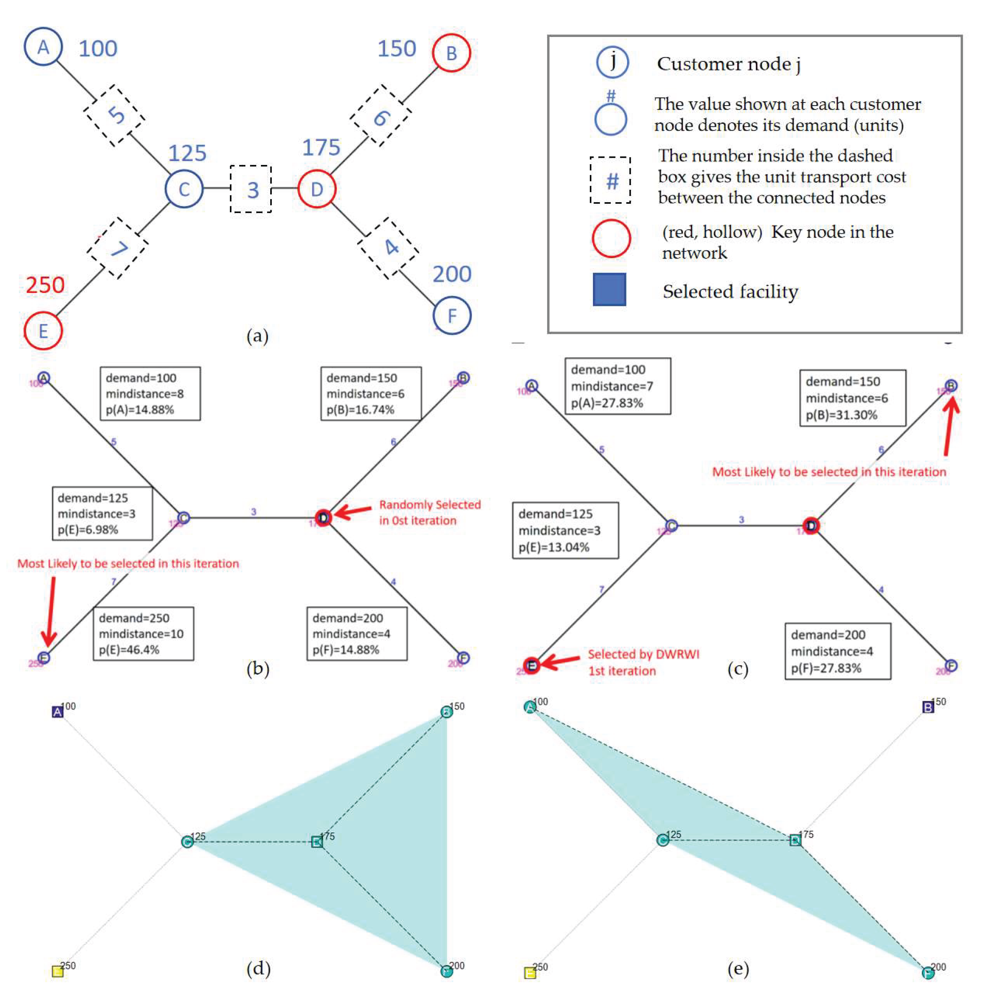
Figure 3.
Large Case Performance Comparison Across Methods.
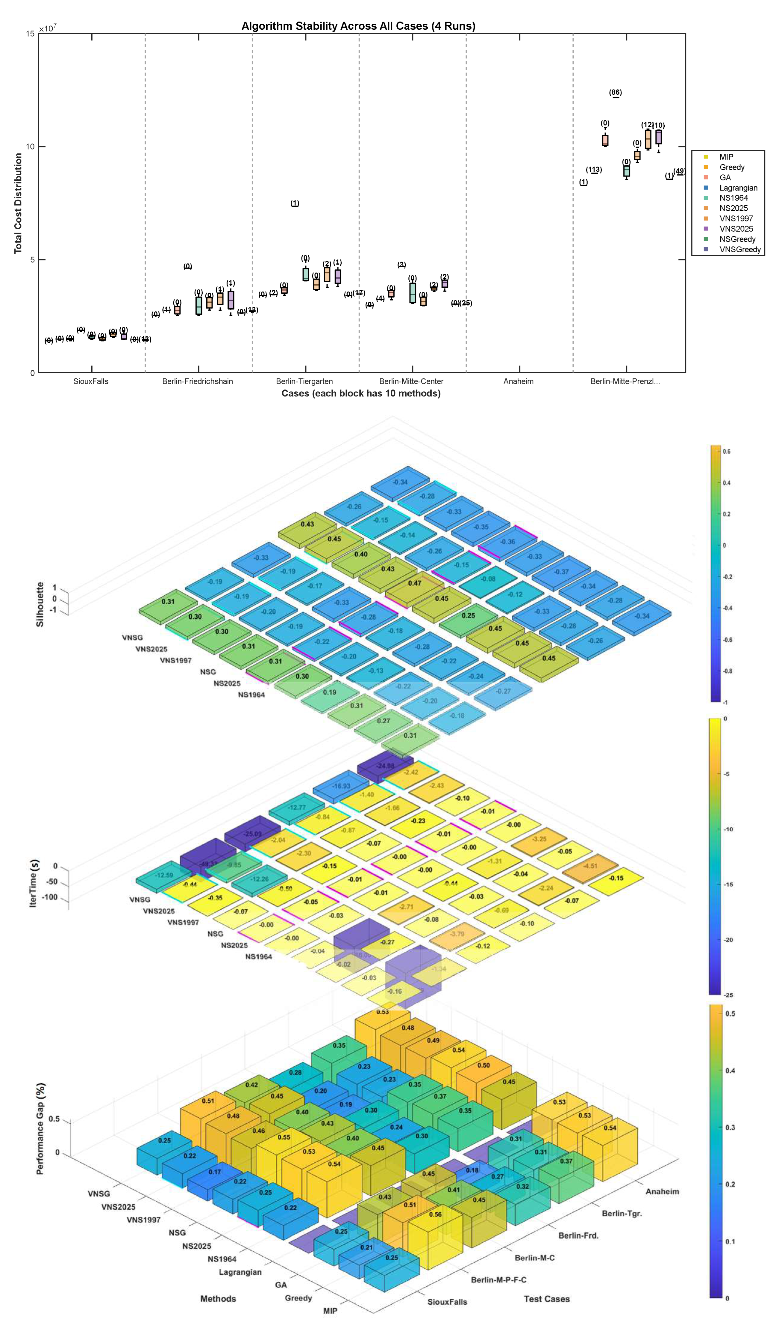
Figure 4.
Warehouse Location Analysis on the SiouxFalls Network:(a) DWRWI Location Construction Result; (b) VNS2025 Location Improvement Result; (c) RI Location Construction Result; (d) VNS1997 Location Improvement Result; (e) GI Location Construction Result; (f) VNSG Location Improvement Result.
Figure 4.
Warehouse Location Analysis on the SiouxFalls Network:(a) DWRWI Location Construction Result; (b) VNS2025 Location Improvement Result; (c) RI Location Construction Result; (d) VNS1997 Location Improvement Result; (e) GI Location Construction Result; (f) VNSG Location Improvement Result.
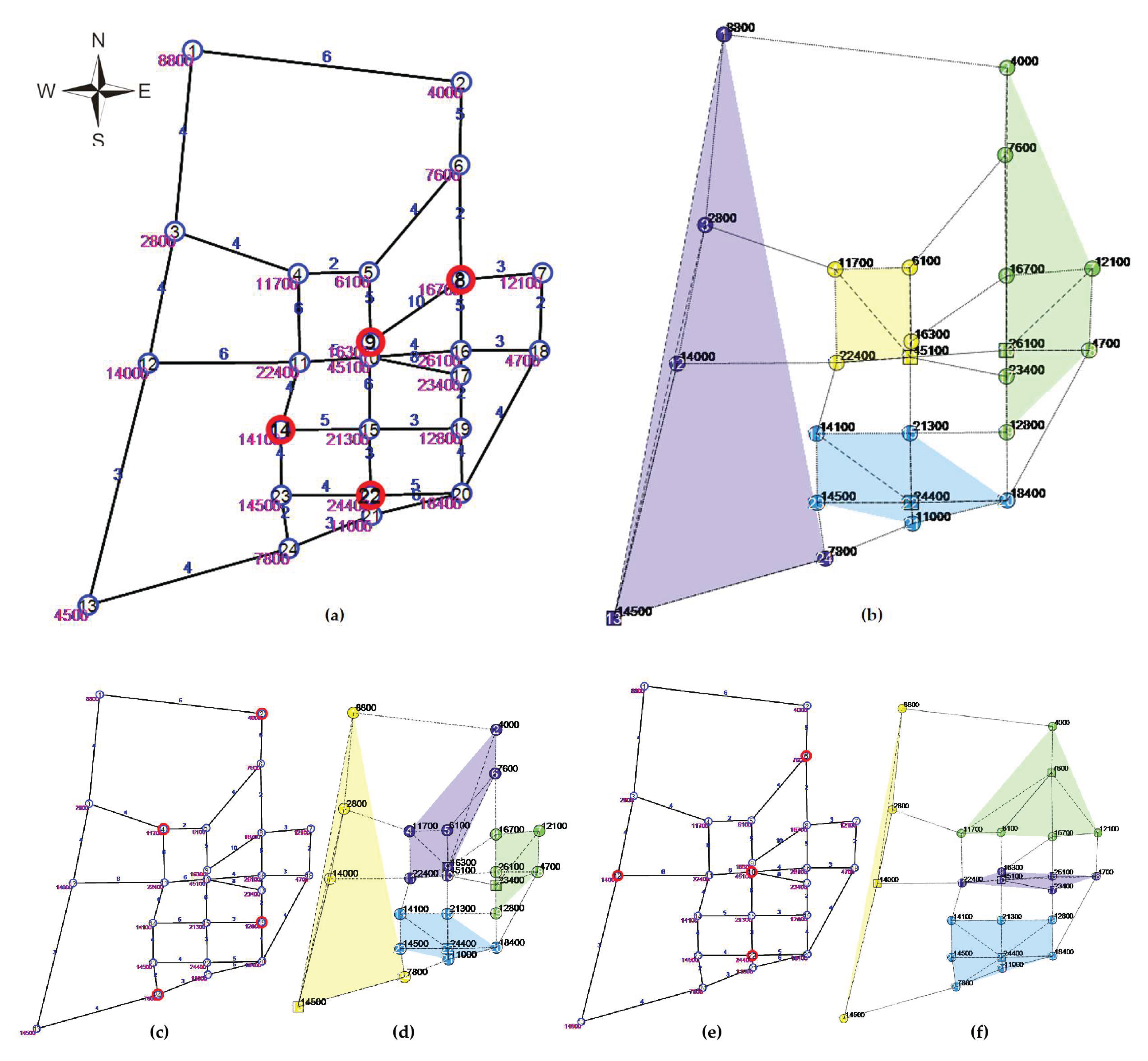
Disclaimer/Publisher’s Note: The statements, opinions and data contained in all publications are solely those of the individual author(s) and contributor(s) and not of MDPI and/or the editor(s). MDPI and/or the editor(s) disclaim responsibility for any injury to people or property resulting from any ideas, methods, instructions or products referred to in the content. |
© 2025 by the authors. Licensee MDPI, Basel, Switzerland. This article is an open access article distributed under the terms and conditions of the Creative Commons Attribution (CC BY) license (http://creativecommons.org/licenses/by/4.0/).
Copyright: This open access article is published under a Creative Commons CC BY 4.0 license, which permit the free download, distribution, and reuse, provided that the author and preprint are cited in any reuse.


