
Submitted:
02 June 2025
Posted:
03 June 2025
You are already at the latest version
Abstract
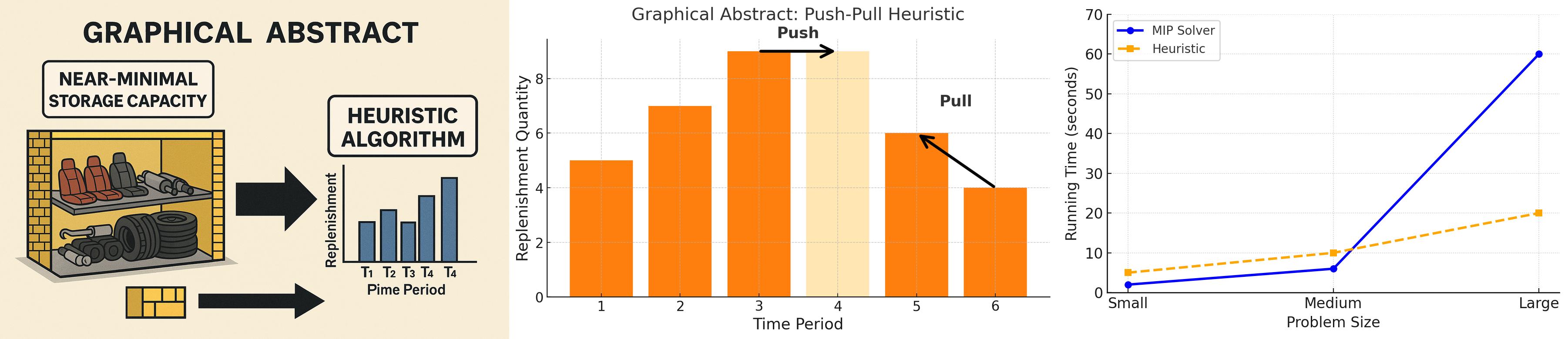
This study aimed to develop an effective heuristic for solving multi-item uncapacitated lot-sizing problems with near-minimal storage capacities. For the initial replenished plan, applying network flow based on a dynamic programming approach was used to solve the single-item lot-sizing problem, while the push operation was used to move the replenished quantities of some items from the existing period to consecutive periods under storage capacity constraints for meeting all demands. To improve the replenished plan, the pull operation was used to return some replenished quantities from the existing period to the previous one and meet all demands together. The results of the random experiment example showed that the proposed heuristic generated differences of 1.20%, 0.63%, and 0.54% between its solutions and the optimal solution with additional storage capacity parameters of 5%, 10% and 20%, respectively. This heuristic effectively solves all random instances of the worst-case conditions for robust operation with the near-minimal storage capacities. For large-scale problems, the proposed heuristic performed well on small gaps between the approximate and optimal solution using less running time with near-minimal storage capacity. Meanwhile, the MIP solver still enhances the running of small and medium-scale problems with near-minimal storage capacity in the shortest run time.
Keywords:
multi-item
; lot size
; near-minimal storage capacity
; replenishment plan
1. Introduction
In supply chain management, the inventory bound, or limitation storage is an im-portant constraint. Raw materials cannot be stored in huge volumes, although the unit price of a raw material unit is low. If raw materials have many different items and stock-keeping units (SKUs), it results in complex problems. Supply chain management decisions depend on the procurement policy of the organization. It comprises operating on minimum inventory cost while considering whether or not to use an expanded storage. An expanded storage area is a feasible solution, which operates at the lowest inventory cost. However, the investment cost for land lease and acquisition, including the rack and shelving supply, must be considered as well. In the case of not considering an expanded storage area, there are two feasible solutions. Firstly, when inventory is over, it must be kept in another area, such as the production line; notwithstanding, this result is with late disbursement, lost materials, and incorrect counting of the number of remaining materials. Total inventory cost is still low. Secondly, keep the amount of inventory under the storage capacity, but the order frequency must grow evidently. As a result, the storage cost continues to be high. When the number of items or SKUs increase, deciding how much of each item to order without exceeding capacity becomes more difficult. In many process industries such as paper manufacturing, petrochemical manufacturing, refineries, food processing, and pharmaceutical manufacturing, storage capacity has become a limiting factor.
In practice, industries such as trailer assembly processes [11], raw-material perishability in composites [22] must all contend with limited inventory bounds. Tight inventory bounds or near-minimal storage capacities that slightly exceed demand require specialized heuristics. Industries operating under Just-In-Time assembly, such as automotive plants [26], are especially sensitive to these constraints. Therefore, the authors introduce a dynamic programming approach based on network flow to generate an initial replenishment plan for each single item and develop a new heuristic to manage the multi-item lot-sizing problem under near-minimal storage capacities.
Storage capacity has been defined by researchers as comprising two distinct categories, such as: the number of ending inventory only, and the sum of the number for the beginning inventory and replenishment. Firstly, most researchers proposed the storage capacity to be based on the number of ending inventory only. Secondly, other researchers introduced the storage capacity to be the total of the number of the beginning inventory and replenishment. Thus, many researchers have defined inventory as the quantity of goods on hand at the end of a specific period. However, in the real world problem, raw material stores usually receive the replenishment at the beginning of the period and keep the inventory of the previous period together to be not over the storage capacity. Consequently, this paper suggests that the total number of inventory in each period depends on the sum of inventory and replenishment at the beginning of the period. There are two definitions of storage capacity: one based on the number of ending inventory, and the other on the sum of beginning inventory plus replenishment. These different definitions not only affect how inventory is calculated but also directly impact the formulation of inventory planning models. As a result, various algorithms have been developed to solve these models.
Lot sizing problems are typically solved using exact methods such as MIP , dynamic programming and heuristic techniques. The earliest known MIP formulation for the lot-sizing problem in the U. S. petroleum refining industry was introduced by Manne [18] in 1958. In his seminal paper, he presented a mathematical model for the dynamic lot-sizing problem, which develop in production planning and inventory control. Meanwhile,Wagner and Whitin [19] introduced a forward algorithm based on the dynamic programming approach to search for optimal lot size decisions. They established the optimal lot sizes for a single item when demand, inventory holding charges, and setup costs change over time. For the management of procurement of materials with storage capacity, consider both the single item and multi-item.
The dynamic programming approach have been implemented by various researches to solve the single-item dynamic lot size problem. Love [1] introduced the first dynamic programming formulation for the Economic Lot-Sizing Problem with Bounded Inventory (ELSB), where inventory levels are constrained by the lower and upper bounds. His model considers both production capacities and storage limitations, which are common in practical applications. It solved in O(T3) time considering backlogging, time-dependent inventory bounds and piecewise concave production, and storage costs when T is the number of periods in the planning horizon. Toczylowski [21] presented an efficient O(T2) algorithm for the general single-item dynamic lot-sizing problem with limited inventory levels and nonzero initial and safety stock levels. Loparic et al. [2] derived a dynamic program or the shortest path problem using regeneration intervals to solve a single-item lot-sizing problem with sales constraints and lower bounds on safety stocks. The limitation of this research is that, in practice, safety stock levels often fluctuate. Sedano-Noda et al. [12] introduced an O(T logT) greedy algorithm to provide optimal policies assuming reorder and linear holding costs without setup costs or backlogging. However, the limitation of this research is that it considers only zero setup costs, which is not practical. Liu and Tu [13] proposed the capacity production-planning (CPP) problem where the production quantity was limited by inventory capacity and stockout. This problem occurs in petrochemical and glass manufacturing, crude oil refining, and food processing. They applied a minimum-cost flow algorithm to construct the network. By applying standard successive-shortest-path methods, they achieved an overall time complexity O(T3). Önal et al. [5] modified dynamic programming procedure that restores optimality for the general bounded-inventory lot- sizing problem in O(T2). However, this study did not include any computational experiments to validate the practical performance of the corrected method. Chu and Chu [14] proposed the dynamic programming approach for the inventory-bounded outsourcing and inventory-bounded outsourcing models. These models execute overall complexity time with O(T2 log T) and O(T2), respectively. The limitation of this approach is impractical for planning horizons longer than a few dozen periods. Hwang and Heuvel [15] presented the O(T2) algorithm based on dynamic programming and the Monge property for solving a dynamic lot-sizing problem with backlogging and inventory bounds when general production and inventory cost structures are concave. In addition, they introduced the O(T log T) algorithm using the points-approach and a geometric technique for fixed-charge cost structure as well as the O(T) algorithm using a line-segments approach, including a geometric technique for the fixed-charge cost structure without speculative motives. However, their algorithm does not provide an optimal solution for the ULS-IB problem. Hwang et al. [16] developed the first polynomial-time O(T⁴) dynamic-programming algorithm to solve the single-item deterministic Economic Lot-Sizing problem with lost sales and bounded inventory (ELS-LB), under the assumption that each period’s inventory capacity is fixed. A drawback of their DP algorithm is that it requires a long running time and a large amount of memory to execute. Boonphakdee and Charnsethikul [23] developed a network- flow based on the dynamic programming approach to solve the single-item uncapacitated lot-sizing problem. In this study, the authors introduce their DP algorithm to generate the initial replenishment plan. Atamtürk and Küçükyavuz [3] proposed a linear programming formulation that achieves tighter relaxations for the single-item lot-sizing problem with inventory bounds and fixed costs.. Gutiérrez et al.[20] extended the classical Wagner–Whitin model by time-varying storage capacities and allowing backlogging. They developed a dynamic programming algorithm with time complexity of O(T³), where T is the number of periods in the planning horizon Their algorithm applies only when both the production cost and the holding or stockout cost functions are concave. Guan and Liu [4] introduced two stochastic models for the single-item lot-sizing problem under uncertainty including inventory-bound only and the other both inventory-bound and constant order-capacity constraints. They developed dynamic programming algorithms from them with the time complexity O(T2) and O(T2nLogT), respectivity, where T is the number of time periods and n is the number of possible order capacities. However, stochastic DP requires complete and precise probability distributions of demand for every period. Chu et al. [6] proposed a single-item dynamic lot-sizing model integrating backlogging, outsourcing, and limited inventory. They developed a dynamic programming algorithm that solves the lot-sizing problem in polynomial time with O(T³) time complexity, where T is the number of periods in the planning horizon. As a result, their algorithm cannot support concave setup or volume-discount cost structures. Brahimi et al.[8] introduced the Two-Level dynamic Lot-Sizing Problem with Bounded Inventory (2LLSP-BI), integrating raw-material procurement and finished-product production planning under finite warehouse capacity constraints. They introduced a new Lagrangian-relaxation heuristic which decomposes 2LLSP-BI into N single-item lot-sizing subproblems. Each subproblem is solved by a dynamic programming. The time per Lagrangian iteration is O(N⋅T2+T⋅Imax), where Imax is the number of the capacity bounds. The raw-material inventory has a single static bound, whereas finished-goods storage is unbounded.Finally, Di Summa and Wolsey [24] studied a mixed-integer program that provides a new convex-hull characterization for the single-item discrete lot-sizing problem with a variable upper bound on the initial stock. However, this formulation is in general too large to be practically useful.
In practice, it is hard to handle only a single item in raw-material storage or on the production line. Consequently, managing multiple items can be quite complex. It is difficult to keep each item and to balance holding costs against ordering costs. Heuristic algorithms are commonly used to solve the multi-item dynamic lot-sizing problem. Many researchers have been interested in creating the heuristic algorithm for solving the multi-item uncapacitated lot-sizing problem with inventory bound (MULSP-IB) due to the practical problem in the real world. This problem is like the multi-item capacitated lot-sizing problem (MCLSP), where the items allocate to a machine with a production capacity constraint. The MULSP-IB only has the limitation of on-hand inventory. Dixon and Poh [27] proposed the smoothing approach. They developed the push and pull operations if all weight or volume of inventory is maintained at more than the storage capacity. For the push operation, replenishment in the existing period t is moved to the consecutive period t+1. On the other hand, the pull operation postpones the replenishment in a backward direction from the existing period t to a previous period t-1 so that all the weight or volume of inventory is maintained at less than the storage capacity. This procedure runs in O(n⋅T). The authors apply the principle of this smoothing method to implement the push and pull procedures. The push procedure postpones replenishment from the current period to the next period, whereas the pull procedure shifts it back to the previous period. Moreover, the authors compare this heuristic’s performance against other heuristics. Park [25] studied the two systems together. He presented the solutions of integrated production and distribution planning and investigated the effectiveness of their integration in a multi-plant, multi-retailer, multi-item, and multi-period logistic environment. Additionally, he introduced the optimization models and a heuristic solution for both integrated and decoupled planning. Akbalik et al. [7] improved the dynamic programming running in O (2nTn+1) time with a polynomial growth rate if the number of items (n) is fixed to solve the MULSP-IB. However, the Tn+1 factor makes the algorithm impractical for larger multi-item instances. Gutiérrez et al. [17] extended the smoothing technique of Dixon and Poh[27]. explored the multi-item dynamic lot-sizing problem with storage capacities or inventory bounds. The problem has been presented to bound applying the weight of inventory in a previous period plus the weight of replenishment in the current period. Its average solution is over around 5% of the solution computed by CPLEX. The authors also compare its performance against the proposed heuristics. Melo and Ribeiro [9] presented the multi-item uncapacitated lot-sizing problem with shared inventory bounds. They developed two MIP-based heuristics : a rounding scheme for generating the feasible solution and a relax-and-fix heuristic for improving the solution. These MIP-based heuristics yield only near-optimal solutions on average within about 2-4 % of the true optimum. Witt[10] introduced a mathematical model for the Multi-Level Capacitated Lot-Sizing Problem with Inventory Constraints (MLCLSP-IC). His model integrates capacity bounds at each level of a product Bill-of-Materials and explicit work-in-process inventory limits. Although it is multi-level, the approach supports only a single item per level; it cannot accommodate product families that share capacities or complex Bills of Materials with alternative subassemblies. Finally, heuristics and MIP-based heuristics for solving MULSP-IB are further explained in Table 1 as below.
In Table 1, the researchers considered only limited storage capacity and did not specifically consider on the case of tight capacity constraints. Therefore, the authors are interested in near-minimal storage capacity constraints, which occur in the automotive assembly industry [26].
This study proposes a new heuristic for computing the approximate replenishment plan for multiple items in each period under storage capacity constraints. The novelty of this study considers the proposed procedure, which can be executed effectively under near-minimal or worst-case storage capacity constraint. Storage capacity is defined as the sum of the weight (or volume) of all items carried over from the previous period and the weight (or volume) of all replenishments in the current period. The authors introduce a dynamic programming approach based on network flow [23] to determine the replenishment plan for each item and propose two methods for computing a multi-item replenishment schedule under storage-capacity constraints. The proposed heuristics consist of a push method and a pull method. The push method postpones replenishments forward from period t to period t + k whenever the inventory level in period t exceeds the limited capacity, and repeats this until the inventory in every period does not exceed its capacity. Then the pull method refines the plan by moving replenishments backward from period t to earlier periods
The second section describes the mathematical formulation of MULSP-IB. The proposed heuristic is effective for solving this problem by the modified push and pull operation. It improves comparison with the push operation by Gutiérrez et al. shown in Section 3, and this heuristic is examined by Gutiérrez’s example in Section 4. In Section 5, the randomly generated data has been implemented for solving the different problem sizes. The performance of this proposed heuristic is compared with the result of Gutiérrez et al.’s algorithm and the smoothing method. For the robustness condition, the worst-case condition is analyzed, which is the near-minimal storage capacity. In the sensitivity analysis, varying the storage capacities affects the total cost and inventory levels. Finally, conclusions are provided in Section 6.
2. Problem Description
2.1. Problem Statement
The problem of MULSP-IB can be stated as this: Each demand dit must be partly or entirely replenished at a period t by inventory . In this study, consider that demands and inventory bounds are time-varying, and the total actual weight/volume of inventory is not over storage capacity. The problem is to find the periods and the number of raw materials delivered within these periods. The objective is to construct a replenished plan such that the total cost is minimized.
2.2. Problem Assumptions
Assumptions are provided to define certain parameters and decision variables as follows.
Assumption 1. Storage capacity is the upper bound of stock.
Assumption 2. A replenished item is stored first before it is used to satisfy demand. This means that the inventory at the beginning of a period plus the replenish-ment is the actual inventory at the end of the periods.
Assumption 3. The sum of demand is not over storage capacity in all periods, and the demands are satisfied at the end of the period.
Assumption 4. Number of items is independent of the quantity of demand and the number of procurement planning horizon.
Assumption 5. Initial inventory in the first period and ending inventory in the last period are zero.
Assumption 6. Backlogging is not allowed.
Assumption 7. There is no consideration of lead time.
2.3. Decision Variables and Parameters
Explanation of decision variables and parameters can be noted in the following.
Indices i the number of items indexed from 1 to N t the number of periods indexed from 1 to T
Parameters dit the demand of item i at period t
Di,t the accumulative demand of item i from period t to period T
fi,t the fixed ordering cost of item i at period t
hi,t the holding cost of item i at period t
pi,t the cost of procuring raw materials of item i at period t
Ii,t the inventory level of item i at period t
wi the unit weight of item i
Ut the storage capacity at period t
Decision variables xi,t the procurement quantity of item i at period t Yi,t if the replenishment of item i at period t occurs, Yit is 1. Otherwise, Yit is 0.
2.4 Mathematical Model


The objective function of MULSP-IB minimizes the sum of ordering, purchased and holding costs in constraint (1). Constraint (2) is the balance of the inventory equation. Each purchased unit and inventory unit at the beginning of the period are always kept first, before moving to production/customers following its demand in constraint (3). Constraint (4) link the purchased variables with the binary variables Yit and accumulated demand () of item i from periods t to T . Constraint (5) is the initial inventory in the first period and the ending inventory in the last period are zeroes. Constraint (6) defines the purchased quantity and inventory, which are not negative. In constraint (7), if replenishment occurs at any period, Yit is 1. Otherwise, Yit is 0.
3. The Proposed Heuristic
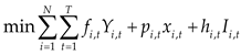
The push and pull strategies of Dixon and Poh [27] consider that excess storage capacity has occurred. This is reduced by moving a replenishment quantity from the existing period t to t+1 when the sum of both inventory and replenishment of all items (SIRallitems) for the existing period is over the storage capacity, called the push operation. On the other hand, a replenishment quantity from period t is returned to a previous period when SIRal litems is less than the storage capacity, called the pull strategy. The push method focuses on reducing SIRallitems in the existing period until success only. Therefore, each iteration enables the reduction of SIRallitems prominently, while ordering cost will grow as necessary, causing total inventory cost to expand as necessary. Furthermore, Gutiérrez et al.’s he ristic extend the push strategy in so far that a replenishment quantity can be moved from any period t to t+k,. For any iteration, Gutiérrez et al.’s heuristic possibly moves a replenishment quantity from a non-existing period to the next period, resulting inSIRallitems in the existing period not also reducing. However, ordering costs still expanding is unnecessary. This study also applies Dixon and Poh’s approach to both the push and pull strategies. For the push strategy, consider a replenishment item in the existing period, which has the maximum sum of inventory and the replenishment quantity (SIRmax). Consider an item of SIRmax condition, called iSIRmax that has an inventory cost of zero at period t+k,called on tzero. Therefore, a replenishment quantity is equal to its demand in the existing period, then it moves so as to add the original replenished quantity at period tzero. After that, the replenishment quantity of the existing item is balanced for all periods. It runs repeatedly until all SIRallitems are less than storage capacities. This procedure is called the push method.
For the pull strategy, find the periods (tmin and tmax) with the minimum and maxi mum differences between SIRallitems and their storage capacities (U), called SIRallitems_Umin and SIRallitems_Umax. If the index of period tmin is higher than the index of period tmax, consider a SIRmin item called iSIRmin for period tmin. Return the replenished quantity, which is the demand of iSIRmin of period tmin, to add the original replenished quantity of the same item at period tmax. Then, calculate all SIRallitems again. If a new SIRallitems for period tmax is still greater than storage capacity at that period, find a new item with SIRmax called iSIRmax. Next, determine the period tzero on iSIRmax and calculate the round-up of the new SIRallitems_U for period tmax divided by its weight, called SIRallitems_Uroundup. Move the replenished quantity, SIRallitems_Uroundup for period tmax, to period tzero. Finally, balance the replenished plan again. This procedure is called the pull method. It can effectively improve the solution generated by the push method. Next, determine the period tzero on iSIRmax and calculate the round-up of the new SIRallitems_U for period tmax divided by its weight, called SIRallitems_Uroundup. Move the replenished quantity, SIRallitems_Uroundup for period tmax, to period tzero. Finally, balance the replenished plan again. This procedure is called the pull method. It can effectively improve the solution generated by the push method. This study proposes a new procedure for solving MULSP-IB. It has a property suggesting that the sum of both the inventory and the replenished quantity for all items (SIRallitems) agree with less storage capacity, satisfying all demands for the existing period or equal storage capacity for that period. This property is presented to clarify the logical flow of arguments as follows:
Theorem 1.
If t is a period such that
for some items i satisfying , , then .
Proof of Theorem 1.
For a contradiction method, the assumption is . Given . It implies that the total inventory is sufficient to satisfy or exceed the storage limitation. However, some and are used to satisfy the demands such that no additional replenishments can exceed the storage limitation. Therefore, there is no additional inventory available to satisfy or exceed the limitation.
Theorem 2.
If t is a period such that for some items i satisfying , , then .
Proof of Theorem 2.
For a contradiction method, let us study a replenishment () that there is an item i, for which the assumption is . In the case of , given , the inventory level and extended replenishments () are not sufficient to satisfy the sum of the consecutive demand (). Further, in the case of , there is additional inventory to be over the storage capacity. However, the given condition does not satisfy the demand. Therefore, the sum of inventory and replenished quantity cannot exceed the storage capacity. To satisfy demand, the sum of the inventory and replenished quantity of all items in each period must either be less than or equal to the storage capacity explained by Theorems 1 and 2, respectively.
3.1. The Push Method
The objective of this method is to seek the approximate solution of MULSP-IB. The procedure for this method can be explained by the pseudo-algorithms as follows:
1: procedure InitialSolution(N, T, U, d, h, f)
2: Input:
3:N← number of items
4:T← number of periods
5:U[1..T] ← inventory bounds per period (network-flow based)
6:d[1..N][1..T] ← demand of item i in period t
7:h[1..N][1..T] ← holding cost of item i in period t
8:f[1..N][1..T] ← ordering cost of item i in period t
9: Output:
10:x[1..N][1..T]← initial replenishment plan
11: for i ← 1 to N do
12:x[i][1..T] ← NetworkFlowDP(i, U, d[i], h[i], f[i])
13: end for
14: return x
15: end procedure
16: procedure PushAlgorithm(N, T, U, d, h, f, x)
17: Input:
18:N← number of items
19:T← number of periods
20:U[1..T] ← storage capacity per period
21:d[1..N][1..T] ← demand of item i in period t
22:x[1..N][1..T] ← initial replenishment plan
23: Output:
24:x[1..N][1..T], TotalCost
25: for t ← 1 to T do
26:// Compute SIR for each item at period t
27:for i ← 1 to N do
28: if t == 1 then
30: else
31: inv[i] ← inv_prev[i] + x[i][t] - d[i][t]
32: end if
33: tailDemand ← 0
34: for k ← t to T do
35: tailDemand ← tailDemand + d[i][k]
36: end for
37: SIR[i] ← inv[i] + tailDemand
38: inv_prev[i] ← inv[i]
39:end for
40:SIRall ← Σ_{i=1..N} SIR[i]
41:slack ← SIRall - U[t]
42:while slack > 0 do
43: iMax ← argmax_{i=1..N} SIR[i]
44: Δ ← d[iMax][t]
45: x[iMax][t] ← x[iMax][t] - Δ
46: if t < T then
47: x[iMax][t+1] ← x[iMax][t+1] + Δ
48: end if
49: // Recompute inventory and SIR
50: SIRall ← 0
51: for i ← 1 to N do
52: if t == 1 then
54: else
55:inv[i] ← inv_prev[i] + x[i][t] - d[i][t]
56: end if
57: tailDemand ← 0
58: for k ← t to T do
59: tailDemand ← tailDemand + d[i][k]
60:end for
61: SIR[i] ← inv[i] + tailDemand
62: inv_prev[i] ← inv[i]
63: SIRall ← SIRall + SIR[i]
64: end for
65: slack ← SIRall - U[t]
66:end while
67: end for
68: // Calculate total cost
69: TotalCost ← 0
70: for i ← 1 to N do
71:for t ← 1 to T do
72: if x[i][t] > 0 then
73: TotalCost ← TotalCost + f[i][t]
74: end if
75: TotalCost ← TotalCost + inv_prev[i] * h[i][t]
76:end for
77: end for
78: return x, TotalCost
79: end procedure
In line no. 16, pseudo code of dynamic programming based on network flow can be shown in Appendix A.1. The logical sequence including selection rules of the push method can be explained in Figure 1.
In Figure 1, the algorithm stops computing if the difference (diff) between the sum of previous inventory plus replenishment quantity (SIRalitem) and the storage capacity (U) for each period is less than or equal to zero. This selection rule determines whether to perform the next step of the algorithm. From the pseudo code, dynamic programming based on network flow algorithm has time complexity that depends on Dmax, the largest demand value across all items i and all time periods t. Therefore, large demand values significantly influence the running time when solving large-scale problems. The push algorithm has time complexity where W is number of iterations of the while loop per period. If the total inventory exceeds the storage capacity by a large amount, many iterations (W) will be needed to reduce the overcapacity ;otherwise, iteration stops. Therefore, in large-scale problems, inventory overcapacity is likely, causing the proposed algorithm to have a high running time. The replenishment plan generated by the push method can be improved to reduce the total cost using the pull method, which will be discussed in the next section.
3.2. The Pull Method
The objective of this method is to improve the replenishment plan, which is computed by the push method. Some replenishments may be returned from the existing period to the previous period so that the sum of inventory and replenished quantity of all items for the previous period is added to equal its storage capacity. The procedure for the pull method shows the pseudocode of algorithms as follows
1: PROCEDURE Pull method
2: INPUT:
3: X [i, t]← initial replenished quantity for item i in period t computed by the push method
4: demand[i, t]← demand of item i in period t
5: SIR[i, t] ← the sum of previous inventory and replenished quantity of item i in period t
6: U← storage capacity for period t
7: w[i, t] ←weight (or size) of item i in period t
8: T←total number of periods
9: OUTPUT:
10: replenishment plan[i, t] ←adjusted replenished quantities
11: inventoryCost ←updated total inventory cost
12: // Compute initial aggregate SIR per period
13: FOR t ← 1 TO T DO
14:SIRallitems[t] ← Σᵢ SIR[i, t]
15:SIRallitems_SC[t] ← Σᵢ (SIR[i, t] · w[i, t])
16: END FOR
17: // Find periods with min/max aggregate SC usage
18: Tmin ← arg minₜ SIRallitems_SC[t]
19: Tmax ← arg maxₜ SIRallitems_SC[t]
20: // Loop until the lightest-loaded period index is not after the heaviest
21: IF Tmax< Tmin DO
22:// 1) Move the smallest-rate demand from Tmin to Tmax
23:i_min ← arg minᵢ SIR[i, Tmin]
24:qty ← demand[i_min, Tmin]
25:X[i_min, Tmax] ← X[i_min, Tmin] + qty
26:X[i_min, Tmin] ← X[i_min, Tmin] - qty
27:// 2) Rebalance and update all metrics
28:CALL UpdateMetrics()
29:// 3) If Tmax still exceeds capacity, boost its replenishment
30:IF SIRallitems_SC[Tmax] > U THEN
31: i_max ← arg maxᵢ SIR[i, Tmax]
32: adjustment ← ⌈SIRallitems_SC[Tmax] / w[i_max, Tmax]⌉
33: X[i_max, Tmax] ← X[i_max, Tmax] + adjustment
34: CALL UpdateMetrics()
35:END IF
36:// 4) Recompute Tmin and Tmax for next iteration
37:Tmin ← arg minₜ SIRallitems_U[t]
38:Tmax ← arg maxₜ SIRallitems_U[t]
39: END IF
40: RETURN (X, inventoryCost)
41: END PROCEDURE
42: // Subroutine to recalculate inventory levels, SIR, aggregate metrics, and cost
43: PROCEDURE UpdateMetrics
44: FOR t ← 1 TO T DO
45:FOR each item i DO
46: // Recompute SIR[i, t] based on new replenishment qty and demand
47: SIR[i, t] ← ComputeSIR(X[i, t], demand[i, t])
48:END FOR
49:SIRallitems[t] ← Σᵢ SIR[i, t]
50:SIRallitems_U[t] ← Σᵢ (SIR[i, t] · w[i, t])
51: END FOR
52: inventoryCost ← ComputeTotalCost(X, demand, holdingCosts, orderingCosts)
53: END PROCEDURE
In Figure 2, the algorithm proceeds to compute an improved solution if the index of the period with the minimum diff (Tmin) is greater than the index of the period with the maximum diff (Tmax). This selection rule determines whether to perform the next step of the algorithm. The push algorithm has time complexity O(N2T2) when L ≤ N·T , where L is the number of loop. The total running time depends on how many iterations L the algorithm performs to balance the load between periods. If L grows large (close to N·T in the worst case), running time can grow quadratically. To explain the heuristic algorithm, the authors use a numerical example to demonstrate it in the next section.
4. A Numerical Example
This study presents the simple example by Gutiérrez et al. [17] to explain the procedure for both proposed methods. Data from this example is shown in Table 2.
4.1. The Initial Solution
4.2. Solution of the Push Method
From Table 3, SIRallitems values of periods 1, 3, and 4 are positive and their SIRallitems values are certainly excess. Next, the replenished quantity for period one is moved as follows. Period 1
Iteration 1
- Select item 1, which has the maximum SIR (SIRmax) of 567, and find period tzero = 5 on item 1, which has an inventory cost of zero.
- Insert the replenished quantity, which equals the demand of item 1 for period tzero =
- 136 units, on a replenished plan on item 1 for period tzero. For balance demand, de
- crease the replenishment of item 1 for period 1 to 567-136 =431 units.
- Balance a replenished plan and update inventory, SIR,SIRallitems, SIRallitems_U, and total inventory cost (see Table 4).
- SIRallitems_U for period 1 is reduced to 987-756 = +231. Afterward, go to steps 1-4.
Iteration 2
- Select item 2, which has SIRmax of 556, and find period tzero = 2 on item 2, which has an inventory cost of zero.
- Insert the replenished quantity, which equals the demand of item 2 for period tzero = 52 units, on a replenished plan on item 2 for period tzero. For balance demand,
- decrease the replenishment of item 2 for period 1 to 139-52 =87 units.
- Balance a replenished plan and update inventory, SIR, SIRallitems, SIRallitems_U, and
- total inventory cost (see Table 5).
- SIRallitems_U for period 2 is still reduced to 779-756 = +23. Then, go to steps 1- 4.
Iteration 3
- Select item 1, which has SIRmax of 431, and find period tzero = 4 on item 1, which has an inventory cost of zero.
- Insert the replenished quantity, which equals the demand of item 2 for period tzero= 106 units, on a replenished plan on item 1 for period tzero. For balance demand, decrease the replenishment of item 1 for period 1 to 431-106 = 325 units.
- Balance a replenished plan and update inventory, SIR,SIRallitems, SIRallitems_U, and total
- inventory cost (see Table 6).
- SIRallitems_U for period 1 is reduced to 673-756 = -83. Stop the iteration and select period 3, which has the SIRallitems_U value of +947. Proceed to steps 1-4 for period 3.
Period 3
Iteration 1
- Select item 2, which has SIRmax of 1,484, and find period tzero = 5 on item 2, which has
- an inventory cost of zero.
- Insert the replenished quantity, which equals the demand of item 2 for period tzero=118 units, on a replenished plan on item 2 at period tzero. For balance demand, decrease the replenishment of item 2 for period 3 to 371-118 = 253 units.
- Balance a replenished plan and update inventory, SIR,SIRallitems, SIRallitems_U,
- and total inventory cost (see Table 7).
- SIRallitems_U for period 3 is still reduced to 1,108-633 = +475. Afterward, go to steps 1- 4.
Iteration 2
- Select item 2, which has SIRmax of 348, and find period tzero = 4 on item 2,
- which has an inventory cost of zero.
- Insert the replenishment, which equals the demand of item 2 at period tzero =
- 142 units on a replenished plan on item 2 at period tzero. For balance demand, decrease the replenishment of item 2 at period 3 to 253-142 = 111 units.
- Balance a replenished plan and update inventory, SIR,SIRallitems, SIRallitems_U,
- and total inventory cost (see Table 8).
- SIRallitems_U for period 3 is reduced to 540-633= = -93. Stop the loop at
- period 3. Then, find the next SIRallitems_U to be positive. However, all SIRallitems_U values are negative and zero (-83, -255, -93, -84, 0). Thereafter, stop all iterations of the push method.
From Table 8, the push method can generate a total inventory cost equal to 8,977. However, the GAMS/CPLEX solver can execute this problem with an optimal solution of 8,521. The gap between these solutions is = 5.35%. This gap is still high. Therefore, this study proposes the pull method to improve the solution.
4.3. Solution of the Pull Method
From Table 8, all SIRallitems_U are negative or zero. Therefore, the pull method can generate an improved replenished plan. The procedure for this method can beexplained as follows.
- Search the SIRallitems_Umin and SIRallitems_SCmax to be -255 and -83 for periods 2 and 1 from Table 8. So,the index of both periods is tmin=2 and tmax=1. So, tmin is more than tmax.
- Find the SIRmin for period tmin to be 208 on item 2 from Table 8. Return the replenishment of item 2 at period 2 to add the original replenished quantity on item 2 for period tmax=1. Thus, the new amount replenished quantity of item 2 for period 1 is 87+52 = 139 units. For balance demand, the replenished quantity of item 2 for period tmin is reduced to zero (see Table 9).
3. Recalculate SIR,SIRallitems, SIRallitems_U, and total inventory cost (see Table 9).
4. SIRallitems_U of item 2 for period 1 (= +125) is still a positive number. Thus, search the item with SIRmax (= 325) excluding item 2 at period 1, to be 1.
5. For reducing SIRallitems_U to zero at period 1, the SIRallitems_U is divided by the weight of item 1 for period 1 (+125 / 1=125) on item 1 at period tmin =2 to be 0+125 = 125 units (see Table 9). For balance demand, reduce the replenishment of item 1 in the previous period (t=1) to be = 325-125 = 200 units.
6. Recalculate SIR,SIRallitems, SIRallitems_U, and total inventory cost (see Table 10).
7. SIRallitems_U of period 1 is zero and SIRallitems_U of period 2 (tmin) is still -255 (see Table 10), which is the same as Table 9.
8. Find the SIRallitems_Umin and SIRallitems_Umax to be -255 and -84 in periods 2 and 3 from Table 10. The index of both periods is tmin=2 and tmax=3. So, tmin is less than tmax. Then, stop the iteration.
Therefore, the inventory cost is effectively improved to 8,683. The GAMS/CPLEX solver can calculate the optimal solution of 8,521 units. Both the proposed heuristic and Gutiérrez et al. [17] can also calculate the approximate solution the same as 8,683 and the smoothing method of Nixon and Poh [27] can run about 9,494 (see Table 11). Its replenished plan is shown in Table 11.
From Table 10 and Table 11, the gaps between the proposed heuristic, Gutiérrez et al. [17], the smoothing method [27], and GAMS/CPLEX are 1.9 %, 1.9 %, and 11.45 %, respectively. Both the proposed heuristic and Gutiérrez et al. [17] execute approximately five replenishment orders, whereas the smoothing method executes about six. Consequently, the smoothing method incurs a higher total inventory cost than the other approaches due to the increased ordering cost. For further testing, Minner[18] recommended generating test instances as follows: products varied between 3 and 10 and periods varied between 4 and 18, demands are drawn from a uniform (or normal) distribution over a specified range (e.g.\ U[0,100], setup costs are drawn similarly (e.g.\ U[50,150], unit production costs are drawn from U[1,10], holding costs are held constant h =1, weights are drawn from U[1,N], and warehouse capacity bounds are taken as a fixed fraction B =10%. In the format for the storage capacity, parameter A is the sum of the demand onall items at period t with the lower bound (B=1%). Authors generate the example data following Minner [18] procedure as shown in Table 12.
A instance of Minner [18] was computed by heuristics and the resulting solutions are presented in Table 13.
In Table 13, the push-and-pull heuristic achieves an optimality gap of approximately 0 %, outperforming Gutiérrez et al. [17], which has a gap of 1.27 %, and the smoothing method [27], with a gap of 1.02 %. The proposed heuristic places about three replenishment orders, whereas both Gutiérrez et al. [17] and the smoothing method place around four. Consequently, the push-and-pull heuristic’s performance is further validated in Section 5 on a set of randomly generated problem instances.
5. Computational Result
For confidence in using heuristics, this study compares the solutions for the proposed heuristic, algorithm by Gutiérrez et al., and GAMS/CPLEX solver. The set of randomly generated problems is identical to the cost framework of Minner [18]. Each problem runs on formatting parameters, as shown in Table 14.
The parameter B is the additional capacity generated from the accumulative demand of period t+1 with the upper bound. If the upper bound is high, such as B = 20%, the problem can be solved more easily. Otherwise, it is more difficult to address. This study implements MATLAB 2024 A software to solve the network flow algorithm based on dynamic programming for the initial solution, the proposed algorithm [28], and Gutiérrez et al.’s algorithm [29].The solution for the MIP model is generated by GAMS 46.3.0 licensed for continuous and discrete problems. An HP Pavilion X360 Notebook running Windows 10 with an Intel Core i7 64-bit processor at 1.99 GHz and 24 GB of RAM was used to execute both the heuristics and MIP formulation. MATLAB software uses general-purpose programming that is more flexible and allows users to apply specified code. For generating the optimization solution, the GAMS/CPLEX solver is concentrated on optimization, which is less flexible but powerful for LP, MIP, and NLP problems [31]. The solution for the GAMS/CPLEX solver compares all the results of the experiment. It can be explained with the solution gap equation below.
5.1. Experiment Results
This study divides the category for the random example into three sub-categories: A small-scale problem based on the number of periods N =6, a medium-scale problem based on the number of periods N=12, and a large-scale problem based on the number of periods N=24. This experiment shows their solution gaps and computation times varying the parameter B in Table 15, Table 16, Table 17 and Table 18, as follows
5.1. Solution Gap
In Figure 3, the average solution gaps for the push and pull algorithm on large-scale problem are 0.55%,0.38%, and 0.20% for parameter B = 5%, 10% and 20%, respectively. Gutiérrez et al.’s heuristic generates solution gaps of about 2.41%, 1.23% and 0.55 %. When comparing the solution gaps, the proposed heuristic performs better than Gutiérrez et al.’s heuristic. The performance of the solution gap depends on the value of parameter B. If parameter B increases, the solution gap is lower . The proposed algorithm can determine the number of replenished quantities to move relaxed while satisfying all demands with a high parameter B. Gutiérrez et al.’s heuristic sometimes moves the replenished quantity from any period to period t+k, when .Ordering cost must be paid more frequently when inserting the replenished quantity for period t+k in more time, causing total inventory cost to grow. Unfortunately, the amount of SIRallitem _U for period t does not also decline. While the push and pull heuristic moves each replenished quantity from period t to a consecutive period only with zero inventory cost, it can certainly reduce the replenished quantity for period t so that the amount of SIRallitems _U reduces.
5.2. Worst Cases Analysis
For the robust condition of the push & pull heuristic, this study introduces the near-minimal storage capacity. The performance of a heuristic depends on the value of the storage capacity. Suppose each storage capacity is likely near the sum of demand for each period, called near-minimal storage capacity. Moving the partial or whole replenished quantities to the next period is difficult.
In Table 15, it is difficult for Gutiérrez et al.’s heuristic to execute any random instances with near-minimal storage capacities. It can calculate only one and two from five and ten instances, such as 20x24, 30x24, and 40x24 problems (NxT). Other solutions cannot satisfy the demand. Meanwhile, the push and pull heuristic can calculate all random instances with these storage capacities. Its solution gap performs well on the small-and medium-scale problem, at about 1.15% and 1.33%, the same as the other instances with high storage capacities (parameter B =5-20%). At the same time, Gutiérrez et al.’s heuristic gap solution is about 3.99% and 5.57%. Therefore, the push and pull heuristic enables computing the replenished plan significantly better with near-minimal storage capacities. For large-scale problems (T=24), MATLAB cannot run on the extension of the number of periods due to being out-of-memory. When increasing the number of periods, its memory usage exceeds 76 GB. The limitation of the system memory space (RAM and swap file) used by MATLAB for this computer is about 76 GB. To strengthen empirical benchmarking and provide better justification, compare the proposed heuristics with additional baseline methods, including the smoothing heuristic [27] , implemented using the state-of-the-art code [31]. The authors compare their solution gap performance, which is shown in Table 19.
In Table 19, the proposed heuristic shows good average gap performance on large-scale problems, such as the 10x24 case, with gaps of about 1.27% and 0.34% under storage capacities B = 1% and 20%, respectively. In comparison, Gutiérrez et al.’s heuristic has gaps of approximately 6.89% and 1.07%, while the smoothing heuristic has gaps of about 5.97% and 1.35%, respectively. As a result, the gap performances of Gutiérrez et al.’s and the smoothing heuristics differ by only a small amount. Therefore, the proposed heuristic is able to compute an approximate replenishment plan that is better than the previous heuristics.
5.3. Computation Time
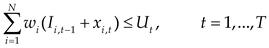
This study implements the codes based on the state-of-the-art methods for both heuristics. Both the push & pull heuristic and the heuristic by Gutiérrez et al. have the same time complexity, denoted as . Therefore, the running times of the two heuristics are nearly the same. The time complexity for the network flow based on dynamic programming algorithm [22] has for generating the initial solution. The computation time of both heuristics combines the running time for the network flow based on dynamic programming for the initial solution with the running time of each heuristic. The worst-case complexity of the GAMS/CPLEX solver has , which is an exponential growth rate. However, this solver enhances performance with the branch-cut and benders decomposition algorithm for reducing the running time efficiency in large-scale problems [28] when compared with MATLAB software. For computation time, this study focuses on small-to-medium and large-scale problems with near-minimal storage capacity. Therefore, the data in Figure 4 include both small-to-medium and large-scale problems (see Table 15) with storage capacities parameter B=1-20%. Both the heuristics and MIP solver generate solutions under storage capacities. The computation time for these conditions is shown in Figure 4, Figure 5, Figure 6 and Figure 7, as follows:
In Figure 4, the computation time generated by the GAMS/CPLEX solver increases exponentially for the large-scale problem under near-minimal storage capacities (B = 1%). In general, the CPLEX solver must execute effectively with a branch-and-cut algorithm and special heuristic. However, the running time for solving a large-scale problem includes poor performance with near-minimal storage capacities. The MIP solver must determine lot size with high running time to generate an optimal solution. This is a limitation of the MIP solver. In contrast, the computation time for both heuristics, which generate approximate solutions for large-scale problems, performs well compared to the MIP solver. Nevertheless, the computation time of the MIP solver on small- to medium-scale and large-scale problems performs well compared to both heuristics when the storage capacities have higher B values (see Figure 5, Figure 6 and Figure 7). The running times for both heuristics are nearly the same due to their similar time complexity.
Therefore, considering the storage capacity constraints, both heuristics perform well under near-minimal capacity for large-scale problems, whereas the MIP solver computes efficiently with shorter running times for small- and medium-scale problems. For high storage capacity constraints (B = 5–20%), the MIP solver performs well with shorter running times across all problem scales.
5.4. Sensitivity Analysis
Authors present a sensitivity analysis on the varied parameter B to show its impact on the cost performance of the proposed heuristics, order frequency, and inventory levels. The results of this analysis are shown in Figure 8, Figure 9 and Figure 10 below.
In Figure 8, the total cost for each problem size is high when the storage capacity is near minimal, and it decreases as the storage capacity increases. Under the near-minimal storage capacity constraint, the inventory level for each problem size is low due to the limited storage space (see Figure 9). This results in more frequent orders with smaller replenishment quantities to meet all demand. The higher order frequency causes an increase in the total cost (see Figure 10).
Under high storage capacity constraints, the total cost for each problem size is low, but the inventory level is higher due to the increased storage space. The order frequency is also lower in order to reduce the total cost.
In summary, tight storage space leads to higher total costs due to increased order frequency. On the other hand, larger storage capacity results in lower total costs but requires higher investment to expand the storage space.
5.5. Statistical Validation of Heuristic Stability and Reliability
For validation of heuristic stability and reliability, the authors evaluate the total cost and running time of the proposed heuristic using statistical parameters such as average, standard deviation, minimum and maximum values, and confidence intervals, as shown in Table 20.
6. Conclusions
This study proposes a novel push-pull heuristic for solving the multi-item un-capacitated lot-sizing problem under near-minimal storage capacities. When capacity constraints are nearly minimal across multiple items, novel heuristics are required. Pior heuristics did not directly consider the tight storage capacity constraints. The just-in-time operation in the assembly automobile industry is difficult to share the storage capacity on the multi-item parts. The proposed heuristic can be applied to manage tight storage capacity while keeping multiple items. To compute the initial replenishment plan, authors implement a dynamic programming based on network flow to generate a single-item lot size plan for all periods under unlimited storage capacity of each period. The push procedure identifies iteratively the maximal sum of beginning inventory plus the replenishment quantity which moves to the next period without violating the near -minimal storage capacity. Each iteration will increase inventory cost with the ordering cost .The push and pull procedure requires fewer iterations during computation. In comparison, Gutiérrez et al.’s heuristic selects successive periods, resulting in more iterations and increased ordering costs to meet the near-minimal capacity constraints. The result of computation shows that the proposed heuristic performs well on the gap solution under near-minimal storage capacities. The running time of the proposed heuristic performs well on large-scale problem, whereas GAMS/CPLEX solver run with minimal run time on small-and medium-scale problem. However, in the sensitivity analysis, a near-minimal storage capacity constraint results in high inventory costs due to the increased frequency of orders. Future research could expand this proposed heuristic for applying this proposed heuristic then evaluating in a assembly automobile plant to improve the practical applicability and credibility. Another extension, it could run with the stochastic demand or lead time constraints to make it applicable across a wider range of academic settings.
Author Contributions
Conceptualization, W.B. and D.H. and P.C.; methodology, W.B. and D.H.; software, W.B.; validation, W.B. and D.H.; formal analysis, W.B. and D.H.; investigation, W.B. and D.H.; resources, D.H.; data curation, W.B. and D.H.; writing—original draft preparation, W.B. and D.H. ; writing—review and editing, W.B.,D.H. and P.C.; visualization, W.B. and D.H.; supervision, P.C.; projectadministration, W.B. and D.H.; funding acquisition, W.B. and D.H. All authors have readand agreed to the published version of the manuscript
Funding
This study received no external funding.
Data Availability Statement
The data presented in this study are available and can request to the corresponding author.
Acknowledgments
The authors would like to express our sincere appreciations to all constructive comments and recommendations from reviewers leading to theimproved final version of this manuscript. This study was supported by the Faculty of Engineering at Kamphaeng Saen, Kasetsart University, Thailand.
Conflicts of Interest
The authors declare no conflicts of interest.
Appendix A
Appendix A.1
Pseudo code of dynamic programming based on network flow
1: PROCEDURE MultiItemLotSizing
2: // d[N][T] ← demand matrix (rows: items, cols: periods)
3: // order[N][T] ← fixed ordering cost matrix
4: // weight[N]← per-item weight (for capacity constraint)
5: // pc[N][T]← per-unit production cost matrix
6: // h← unit holding cost
7: // Output:
8: // sol[N][T]← lot-sizes for each item and each period
9: // invencost[N] ← total inventory cost per item
10: CONST M ← 10^10// “infinite” penalty
11: CONST extra ← 1// cost offset for indexing
12:
13: FOR g ← 1 TO N DO// for each item
14:// 2. Compute sumdemand and cumdemand
15:FOR k ← 1 TO T DO
16: sumdemand[g][k] ← Σ_{i=1..T} d[g][i]
17:END FOR
19:FOR k ← 2 TO T DO
20: cumdemand[g][k] ← cumdemand[g][k−1] + sumdemand[g][k]
21:END FOR
22:
23:// 3. Build DP network of size S = T + Σ_k sumdemand[g][k] + 1
24:S ← T + Σ_{k=1..T} sumdemand[g][k] + 1
25:ALLOCATE dcost[1..S][1..S]
26:
27:// 4. Fill dcost for “period 0” (building initial inventory)
28:FOR inv ← 0 TO sumdemand[g][1] DO
29: lot ← inv − 0 + 0
30: IF lot > 0 THEN
31: y ← 1
32: ELSE
33: y ← 0
34: END IF
36:END FOR
37:
38:// 5. Fill dcost for periods 1..T−1
39:node_i ← 1
40:FOR p ← 1 TO T−1 DO
41: prev_node_i ← node_i
42: FOR inv_prev ← 0 TO sumdemand[g][p] DO
43: node_i ← prev_node_i + inv_prev
44: FOR inv_curr ← 0 TO sumdemand[g][p+1] DO
45:lot ← inv_curr − inv_prev + d[g][p]
46:IF lot > 0 THEN
47:y ← 1
48:ELSE
49:y ← 0
50:END IF
51:// compute holding penalty
52:IF lot == 0 AND inv_prev − inv_curr == d[g][p] THEN
53:hold ← inv_curr * h
54:ELSE IF lot > 0 AND inv_prev − inv_curr + lot == d[g][p] THEN
55:hold ← inv_curr * h
56:ELSE
57:hold ← M
58:END IF
59:// assemble cost
60:IF hold == M THEN
61:cost ← M
62:ELSE
63:cost ← hold + lot*pc[g][p] + y*order[g][p]
64:END IF
65:dcost[node_i][node_i + sumdemand[g][p+1] + 1] ← cost + extra
66: END FOR
67: END FOR
68: node_i ← node_i + sumdemand[g][p+1] + 1
69:END FOR
70:
71:// 6. Fill dcost for final period T
72:FOR inv_prev ← 0 TO sumdemand[g][T] DO
73: node_i ← node_i + inv_prev
74: lot ← 0 − inv_prev + d[g][T] // end inventory is forced to 0
75: IF lot > 0 THEN
76: y ← 1
77: ELSE
78: y ← 0
79: END IF
80: IF lot == 0 AND inv_prev − 0 == d[g][T] THEN
81: hold ← 0 * h
82: ELSE IF lot > 0 AND inv_prev − 0 + lot == d[g][T] THEN
83: hold ← 0 * h
84: ELSE
85: hold ← M
86: END IF
87: IF hold == M THEN
88: cost ← M
89: ELSE
90: cost ← hold + lot*pc[g][T] + y*order[g][T]
91: END IF
92: dcost[node_i][S] ← cost + extra
93:END FOR
94:
95:// 7. Solve DP by backward recursion
96:ALLOCATE fn[1..S+1] ← 0
97:ALLOCATE fnmat[1..S][1..S]
98:// 7.1 Initialize last column
99:FOR i ← 1 TO S DO
100:fnmat[i][S] ← dcost[i][S]
101: END FOR
102: fn[S] ← MIN_{i=1..S} fnmat[S][i]
103: // 7.2 Recurrence
104: FOR i ← S−1 DOWNTO 1 DO
105:FOR j ← i TO S DO
106: IF dcost[i][j] > 0 THEN
107: fnmat[i][j] ← dcost[i][j] + fn[j+1]
108: END IF
109:END FOR
110:fn[i] ← MIN_{j=i..S} fnmat[i][j]
111: END FOR
112:
113: // 8. Trace optimal path
114: INITIALIZE optimalsol[0..T+1][1..5] ← 0
115: current_node ← 1
116: FOR period ← 0 TO T DO
117:// find next node j where fn[current_node] == fnmat[current_node][j]
118:SELECT smallest j ≥ current_node such that fn[current_node] == fnmat[current_node][j]
119:lot ← corresponding lot-size on arc (current_node→j)
120:inv ← previous_inv − demand + lot
121:optimalsol[period+1] ← (prev_inv, lot, demand, inv, arc_cost − extra)
122:current_node ← j + 1
123: END FOR
124:
125: // 9. Record item-level solution
126: FOR p ← 1 TO T DO
127:sol[g][p] ← max(0, optimalsol[p+1].lot)
128: END FOR
129: invencost[g] ← fn[1] − extra
130: END FOR
131:
132: END PROCEDURE
References
- Love, S.F. Bounded Production and Inventory Models with Piecewise Concave Costs. Manag. Sci. 1973, 20, 313–318. [Google Scholar] [CrossRef]
- Loparic, M.; Pochet, Y.; Wolsey, L.A. The Uncapacited Lot-Sizing Problem with Sales and Safety Stocks. Math. Program. 2001, 89, 487–504. [Google Scholar] [CrossRef]
- Atamtürk, A.; Küçükyavuz, A. Lot Sizing with Inventory Bounds and Fixed Costs: Polyhedral Study and Computation. Oper. Res. 2005, 53, 711–730. [Google Scholar] [CrossRef]
- Guan, Y.; Liu, T. Stochastic Lot-Sizing Problem with Inventory-Bounds an Constant Order-Capacities. Eur. J. Oper. Res. 2010, 207, 1398–1409. [Google Scholar] [CrossRef]
- Önal, M.; Heuvel, W.V.D.; Liu, T. A Note on the Economic Lot Sizing Problem with Inventory Bounds. Eur. J. Oper. Res. 2012, 223, 290–294. [Google Scholar] [CrossRef]
- Chu, C.; Chu, F.; Zhong, F.; Yang, S. A Polynomial Algorithm for a Lot-Sizing Problem with Backlogging, Outsourcing, and Limited Inventory. Comput. Ind. Eng. 2013, 64, 200–210. [Google Scholar] [CrossRef]
- Akbalik, A.; Penz, B.; Rapine, C. Multi-Item Uncapacitated Lot Sizing Problem with Inventory Bounds. Optim. Lett. 2015, 9, 143–154. [Google Scholar] [CrossRef]
- Brahimi1, N.; Absi, N.; Dauzère-Pérès, S.; and Kedad-Sidhoum, S. Models and Lagrangian Heuristics for a Two-Level Lot-Sizing Problem with Bounded Inventory. OR Spectrum. 2015, 37, 983–1006. [Google Scholar] [CrossRef]
- Melo, R.A.; Ribeiro, C.C. Formulations and Heuristics for the Multi-Item Uncapacitated Lot-Sizing Problem with Inventory Bounds. Int. J. Prod. Res. 2015, 55, 576–592. [Google Scholar] [CrossRef]
- Witt, A. A Heuristic for the Multi-Level Capacitated Lot Sizing Problem with Inventory Constraints. Int. J. Manag. Sci. Eng. Manag. 2019, 14, 249–252. [Google Scholar] [CrossRef]
- Mohammadi, A.; Shegarian, E. A Mixed Integer Linear Programming Model for the Multi-Item Uncapacitated Lot-Sizing Problem: A case study in the trailer manufacturing industry. Int. J. Multivar. Data Anal. 2017, 1, 173–199. [Google Scholar] [CrossRef]
- Sedeno-Noda, A.; Gutierrez, J.; Abdul-Julbar, B.; Sicilia, J. An O (T log T) Algorithm for the Dynamic Lot Size Problem with Limited Storage and Linear Costs. Comput. Optim. Appl. 2004, 28, 311–323. [Google Scholar] [CrossRef]
- Liu, X.; Tu, Y. Production Planning with Limited Inventory Capacity and Allow Stockout. Int. J. Prod. Econ. 2008, 111, 180–191. [Google Scholar] [CrossRef]
- Chu, F.; Chu, C. Single-Item Dynamic Lot-Sizing Models with Bounded Inventory and Outsourcing. IEEE Trans. Syst. Man. Hum. 2008, 38, 70–77. [Google Scholar] [CrossRef]
- Hwang, H.-C.; Heuvel, W.V.D. Improved Algorithms for a Lot-Sizing Problem with Inventory Bounds and Backlogging. Nav. Res. Logist. 2012, 59, 244–253. [Google Scholar] [CrossRef]
- Hwang, H.-C.; Heuvel, W.V.D.; Wagelmans, A.P.M. The Economic Lot- Sizing Problem with Lost Sales and Bounded Inventory. IIE Trans. 2013, 45, 912–924. [Google Scholar] [CrossRef]
- Gutiérrez, J.; Colebrook, M.; Abdul-Jalbar, B.; Sicilia, J. Effective Replenishment Policies for the Multi-Item Dynamic Lot- Sizing Problem with Storage Capacities. Comput. Oper. Res. 2013, 40, 2844–2851. [Google Scholar] [CrossRef]
- Minner, S. A Comparison of Simple Heuristics for Multi-Product Dynamic Demand Lot-Sizing with Limited Warehouse Capacity. Int. J. Prod. Econ. 2009, 118, 305–310. [Google Scholar] [CrossRef]
- Wagner, H.M.; Whitin, T.M. Dynamic Version of the Economic Lot Size Model. Manag. Sci. 1958, 5, 89–96. [Google Scholar] [CrossRef]
- Gutiérrez, J.; Sedeño-Noda, A.; Colebrook, M.; Sicilia, J. A Polynomial Algorithm for the Production/Ordering Planning Problem with Limited Storage. Comput. Oper. Res. 2007, 34, 934–937. [Google Scholar] [CrossRef]
- Toczylowski, E. An O(T2) Algorithm for the Lot-Sizing Problem with Limited Inventory Levels. In Proceedings of the International Conference on Emerging Technologies and Factory Automation (ETFA), Paris, France, 10–13 October 1995; p. 78. Available online: https://ieeexplore.ieee.org/stamp/stamp.jsp?tp=&arnumber=496709&tag=1 (accessed on 9 September 2024).
- Ojeda, A. Multi-level production planning with raw-material perishability and inventory bounds. Ph.D. Thesis, (Industrial Engineering) of Concordia University, Montreal, Canada, September 2019. [Google Scholar]
- Boonphakdee, W.; Charnsethikul, P. Column Generation Approach for Solving Uncapacitated Dynamic Lot-Sizing Problems with Time-Varying Cost. Int. J. Math. Oper. Res. 2022, 23, 55–75. [Google Scholar] [CrossRef]
- Di Summa, M.; Wolsey, L.A. Lot-Sizing with Stock Upper Bounds and Fixed Charges. SIAM J. Discret. Math. 2010, 24, 853–875. [Google Scholar] [CrossRef]
- Park, Y.B. An Integrated Approach for Production and Distribution Planning in Supply Chain Management. Int. J. Prod. Res. 2005, 43, 1205–1224. [Google Scholar] [CrossRef]
- Emde, S. Sequencing Assembly Lines to Facilitate Synchronized Just-In-Time Part Supply. J. Sched. 2019, 22, 607–621. [Google Scholar] [CrossRef]
- Dixon, P.S.; Poh, C.L. Heuristic Procedures for Multi-Item Inventory Planning with Limited Storage. IIE Trans. 1990, 22, 112–123. [Google Scholar] [CrossRef]
- MATLAB code for Heuristic for the multi-item lot-sizing with storage capacities. MATLAB Central File Exchange. Available online: https://www.math works.com/matlabcentral/fileexchange/179289-heuristic-for-the-multi-item-lot-sizinng-with-storage-cap (accessed on 18 January 2025).
- MATLAB code for Heurictic of Gutierrez et al. 2013 algorithm. MATLAB Central File Exchange. Available online: https://www.mathworks.com/matlabcentral/fileexchange/179294-heurictic-of-gutierrez-et-al-2013-algorithm (accessed on 18 January 2025).
- MATLAB code for Smoothing Heuristic Multi-item Lot size with Storage cap. MATLAB CentralFile Exchange. Available online: https://www.mathworks.com/matlabcentral/fileexchange/181148-smoothing-heuristic-multi-item-lot-size-with-storage-cap (accessed on 15 May 2025).
- CPLEX solver. Available online: https://documentation.aimms.com/platform/solvers/cplex.html (accessed on 23 December 2024).
Figure 1.
Flow chart of the push method.
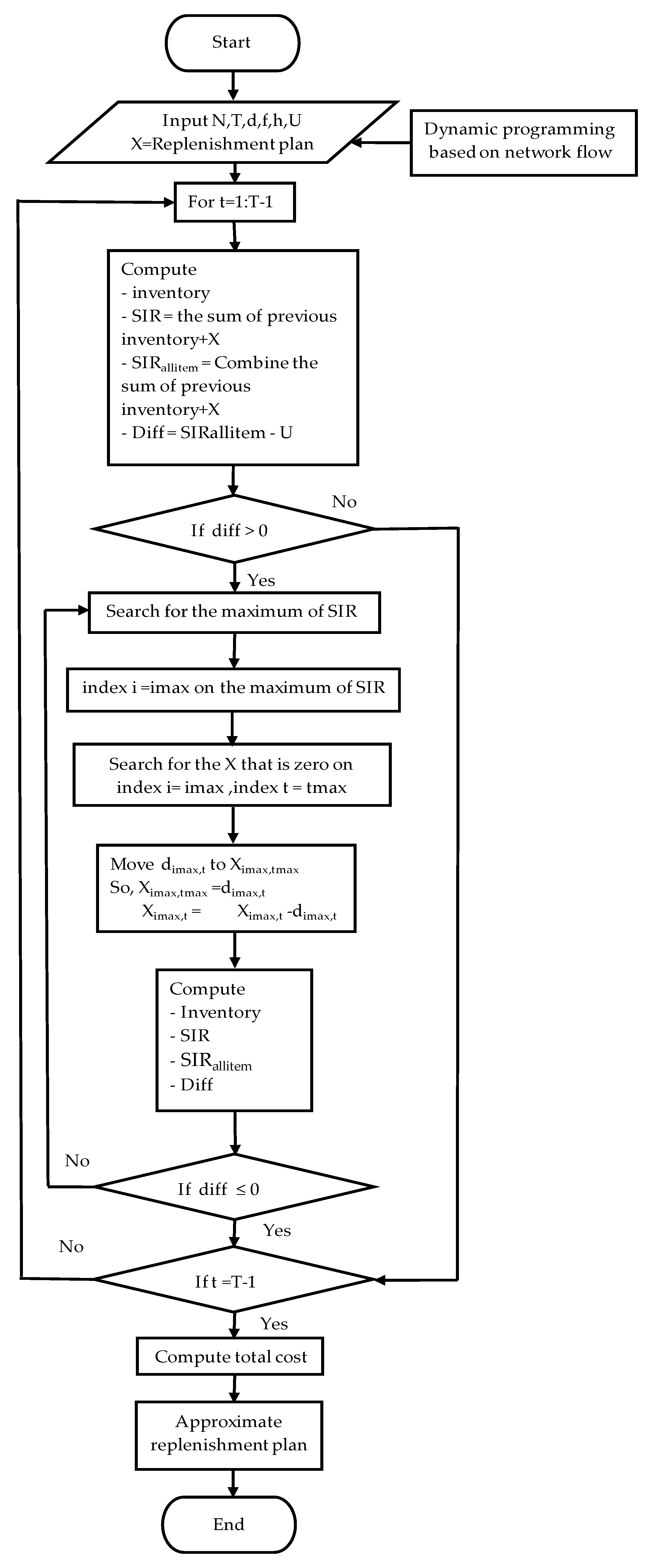
Figure 2.
Flow chart of the pull method.
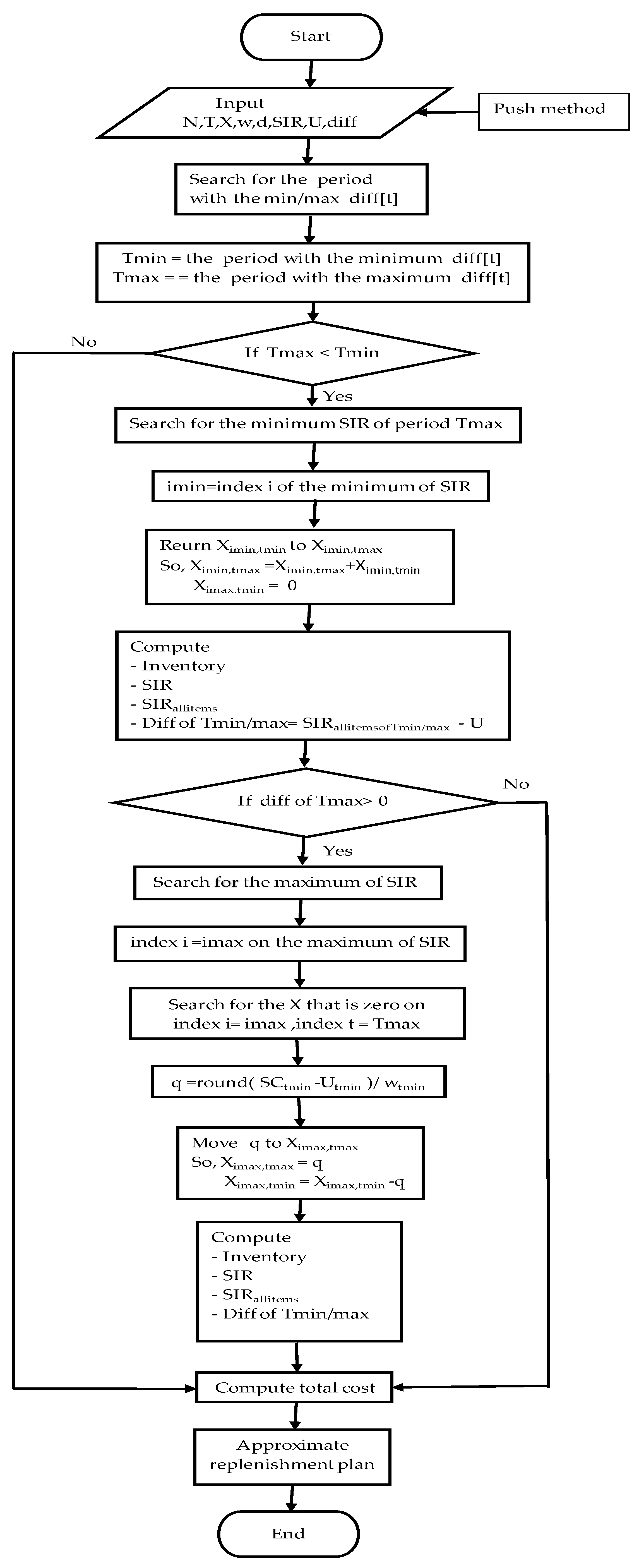
Figure 3.
Average solution gap of both heuristics under storage capacities when parameter B=1,5,10 and 20%.
Figure 3.
Average solution gap of both heuristics under storage capacities when parameter B=1,5,10 and 20%.
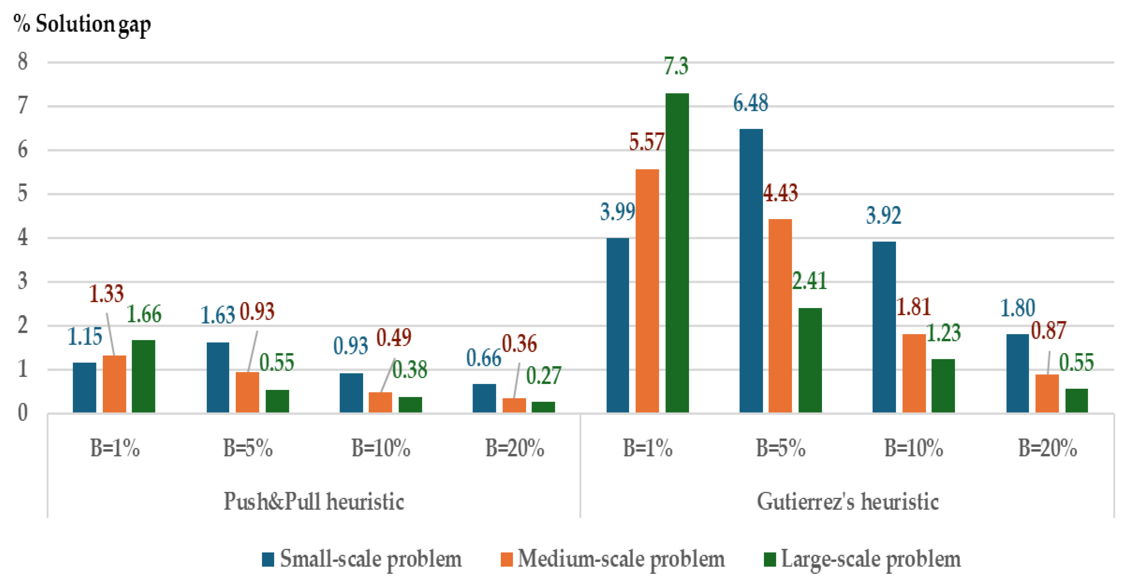
Figure 4.
Average computation time with near-minimal storage capacity (B=1%) using a) push and pull heuristic b) Gutiérrez et al.’s heuristic, , and c) GAMS/CPLEX solver.
Figure 4.
Average computation time with near-minimal storage capacity (B=1%) using a) push and pull heuristic b) Gutiérrez et al.’s heuristic, , and c) GAMS/CPLEX solver.
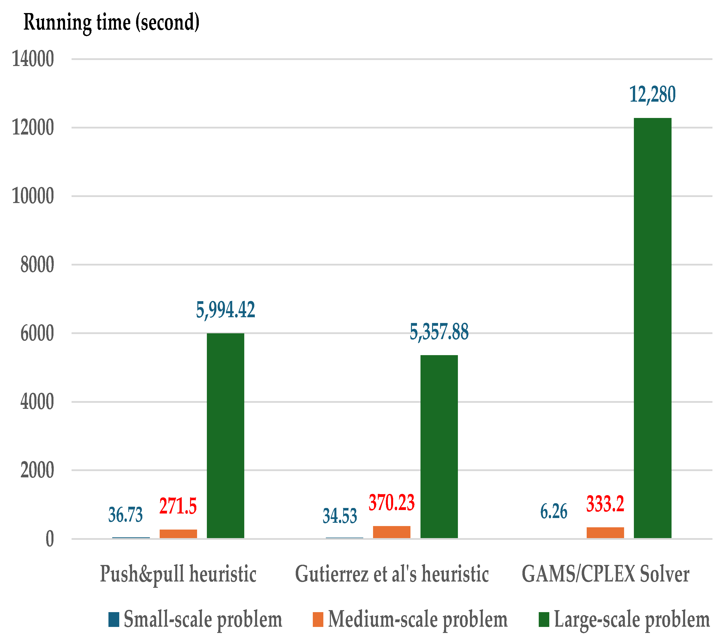
Figure 5.
Average computation time with near-minimal storage capacity (B=5%) using a) push and pull heuristic b) Gutiérrez et al.’s heuristic, , and c) GAMS/CPLEX solver.
Figure 5.
Average computation time with near-minimal storage capacity (B=5%) using a) push and pull heuristic b) Gutiérrez et al.’s heuristic, , and c) GAMS/CPLEX solver.
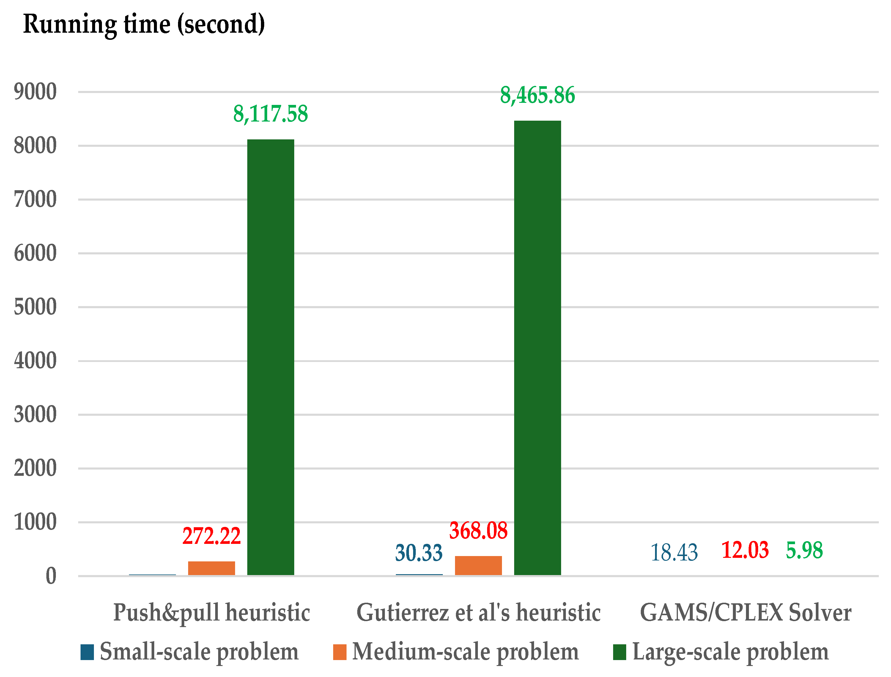
Figure 6.
Average computation time with near-minimal storage capacity (B=10%) using a) push and pull heuristic b) Gutiérrez et al.’s heuristic, , and c) GAMS/CPLEX solver.
Figure 6.
Average computation time with near-minimal storage capacity (B=10%) using a) push and pull heuristic b) Gutiérrez et al.’s heuristic, , and c) GAMS/CPLEX solver.
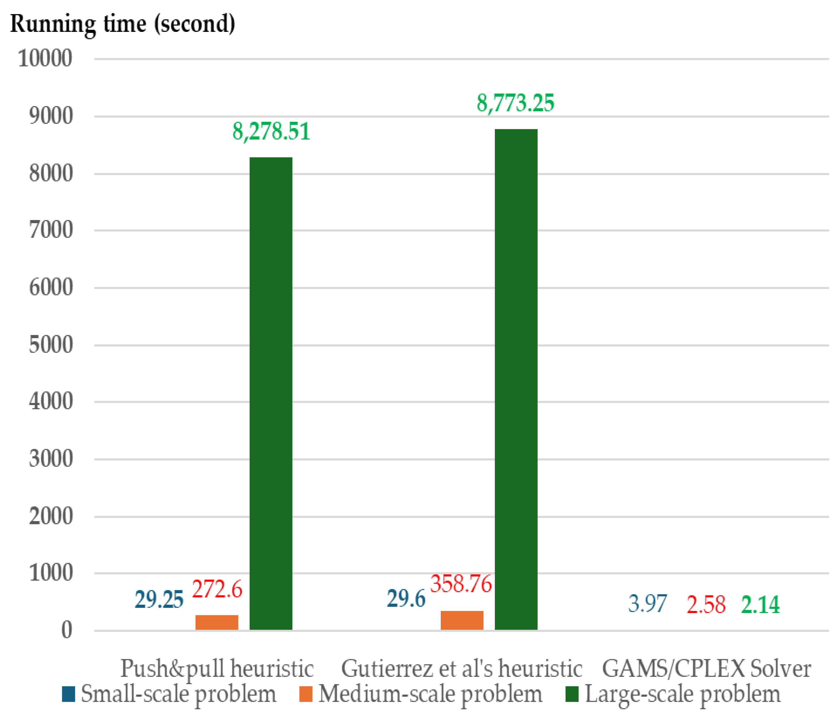
Figure 7.
Average computation time with near-minimal storage capacity (B=20%) using a) push and pull heuristic b) Gutiérrez et al.’s heuristic, and c) GAMS/CPLEX solver.
Figure 7.
Average computation time with near-minimal storage capacity (B=20%) using a) push and pull heuristic b) Gutiérrez et al.’s heuristic, and c) GAMS/CPLEX solver.
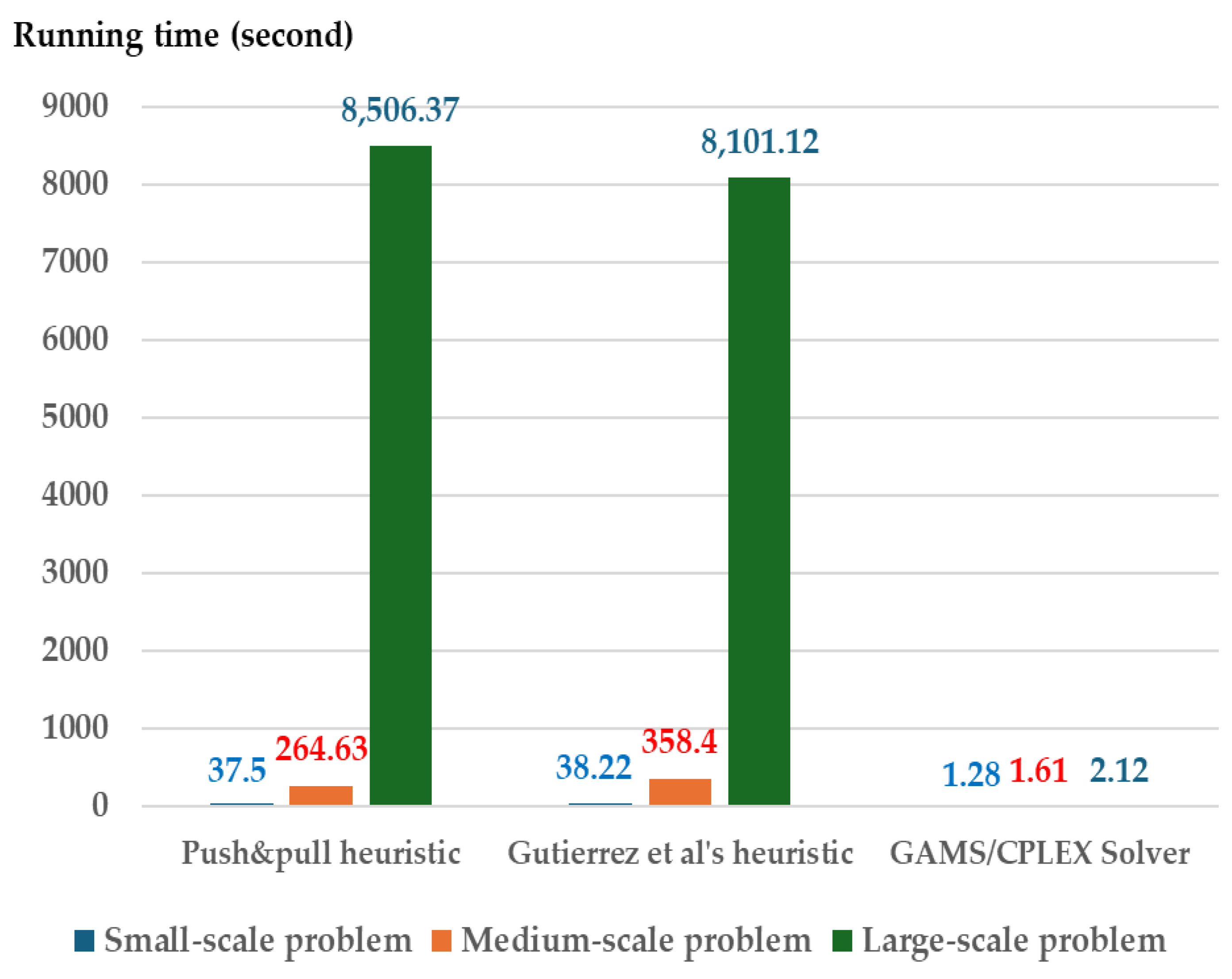
Figure 8.
Total cost vs. storage capacity parameter B (1%–20%) for different problem Scales.
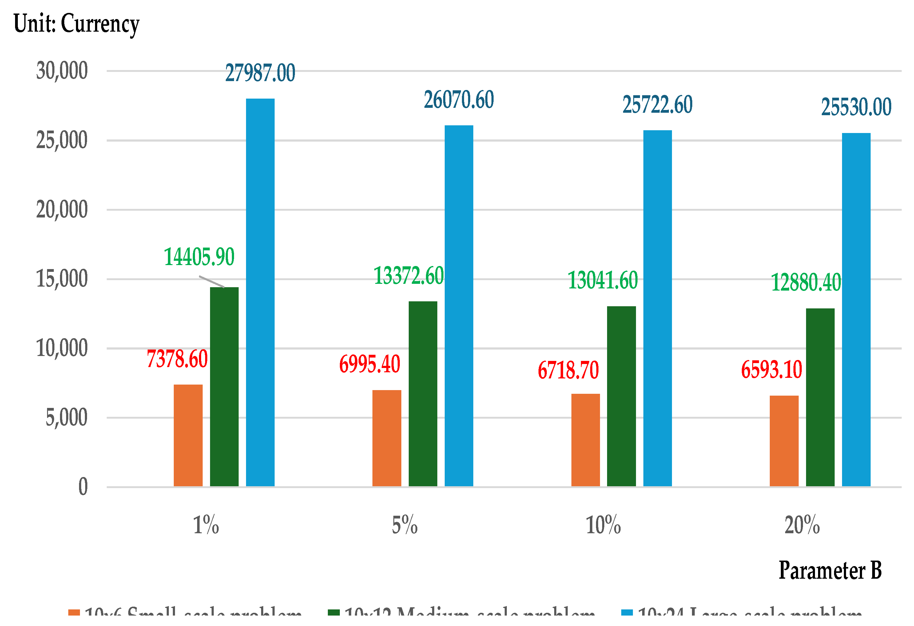
Figure 9.
Inventory level vs. storage capacity parameter B (1%–20%) for different problem scales
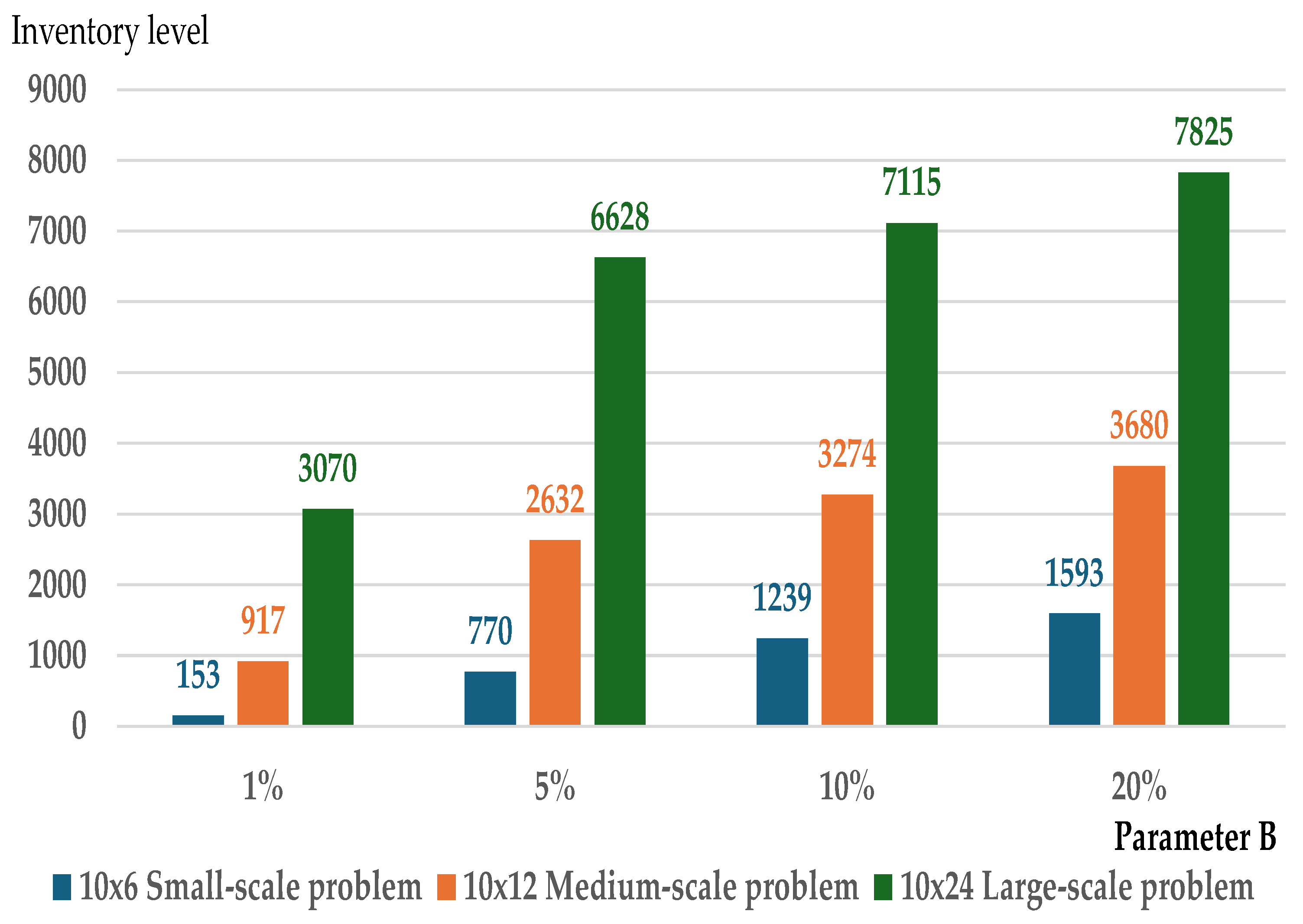
Figure 10.
Order frequency vs. storage capacity parameter B (1%–20%) for different problem scales.
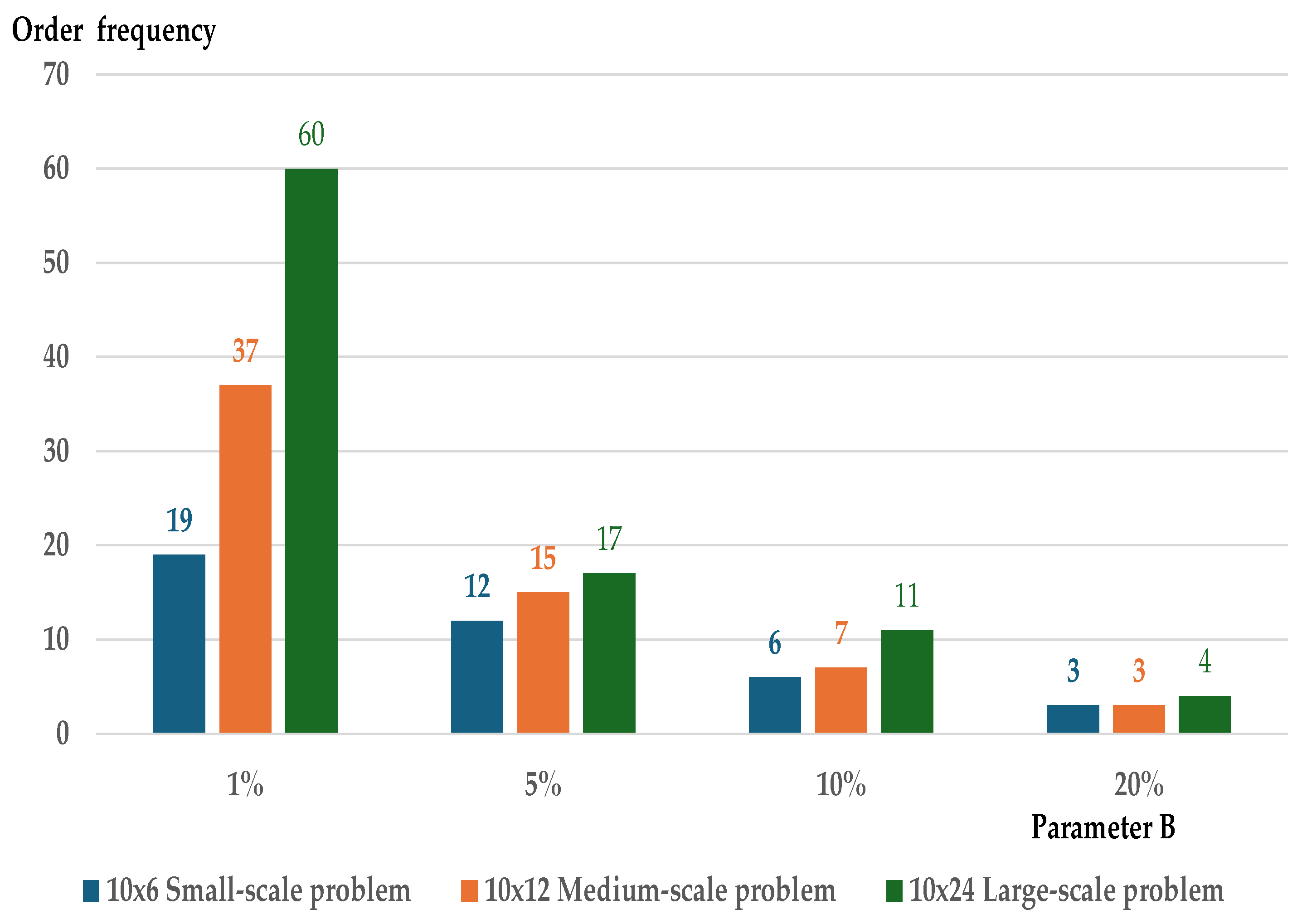

Table 1.
A systematic overview of heuristics and MIP-based approaches.
| References | Model. | Stor. | Algo. | Cap. |
|---|---|---|---|---|
| Dixon and Poh[27] | I&P | BegInv. | DP.&Heu. | Limit.Inv. |
| Park[25] | I&P&R&V | EndInv. | LR.Heu. | Limit.Inv&P&R |
| Akbalik et al. [7] | I&P | EndInv. | DP. | Limit.Inv. |
| Gutiérrez et al. [17] | I&P | BegInv. | DP.&Heu. | Limit.Inv. |
| Melo and Ribeiro [9] | I&P&PT&V | EndInv. | LP.R.Heu.&Heu. | Limit.Inv. |
| Witt[10] | I&P | EndInv. | Heu. | Limit.Inv. |
Abbreviations, Model. Model formulation I&P = inventory and production constraints; I&P&R&V = inventory,production,retailer and vehicle ; &P&PT&V = inventory,production,production time and vehicle constraints constraints; Stor. Storage capacity EndInv.= ending inventory BegInv.= sum of beginning inventory and replenishment Algo. Algorithm DP.= Dynamic programming DP.&Heu.= Dynamic programming and heuristic. LR.Heu.= Lagrangian-relaxation-based heuristic ; LP.Heu.&Heu = Linear programming-relaxation-based heuristic and heuristic Heu. = Heuristic; Cap. CapacityLimit.Inv = Limited inventory constraint Limit.Inv&P&R= Limited inventory,plant and vehicle.
Table 2.
A simple example by Gutiérrez et al. [17].
Table 2.
A simple example by Gutiérrez et al. [17].
| Periods t | 1 | 2 | 3 | 4 | 5 |
|---|---|---|---|---|---|
| Ut | 756 | 673 | 633 | 758 | 608 |
| Item 1,w1=1 | |||||
| d1,t | 115 | 114 | 96 | 106 | 136 |
| D1,t | 567 | 452 | 338 | 242 | 136 |
| f1,t | 595 | 100 | 969 | 240 | 945 |
| p1,t | 4 | 7 | 9 | 10 | 4 |
| h1,t | 1 | 1 | 1 | 1 | 1 |
| Item 2,w1=4 | |||||
| d2,,t | 87 | 52 | 111 | 142 | 118 |
| D2,t | 510 | 423 | 371 | 260 | 118 |
| f2,t | 255 | 696 | 125 | 637 | 249 |
| p2,t | 3 | 3 | 0 | 8 | 4 |
| h2,t | 1 | 1 | 1 | 1 | 1 |
Table 3.
Initial solution for each item.
| Periods t Item | 1 | 2 | 3 | 4 | 5 | |
|---|---|---|---|---|---|---|
| Replenished plan | 1 | 567 | 0 | 0 | 0 | 0 |
| 2 | 139 | 0 | 371 | 0 | 0 | |
| Inventory | 1 | 452 | 338 | 242 | 136 | 0 |
| 2 | 52 | 0 | 260 | 118 | 0 | |
| Inventory cost | 1 | 4x567+1x452+595 =3,315 |
338 | 242 | 136 | 0 |
| 2 | 3x139+1x52+255 =724 | 0 | 385 | 118 | 0 | |
| Sum of inventory and replenishment (SIR) | 1 | 567x1=567 | 452 | 338 | 242 | 136 |
| 2 | 139x4=556 | 208 | 1,484 | 1,040 | 472 | |
| SIRallitems | 1,123 | 660 | 1,822 | 1,282 | 608 | |
| SC | 756 | 673 | 633 | 758 | 608 | |
| SIRallitems_U | +367 | -13 | 1,189 | 524 | 0 | |
Table 4.
Execution flow of iteration 1 for period 1 using the push method.
| Periods t | Item | 1 | 2 | 3 | 4 | 5 |
|---|---|---|---|---|---|---|
| Replenished plan | 1 | 567-136=431 | 0 | 0 | 0 | 136 |
| 2 | 139 | 0 | 371 | 0 | 0 | |
| Ending inventory |
1 | 316 | 202 | 106 | 0 | 0 |
| 2 | 52 | 0 | 260 | 118 | 0 | |
| Inventory cost | 1 | 4x431+1x316+595 =2,635 |
202 | 106 | 0 | 1,489 |
| 2 | 724 | 0 | 385 | 118 | 0 | |
| Sum of inventory and replenishment (SIR) |
1 | 1x431=431 | 316 | 202 | 106 | 136 |
| 2 | 556 | 208 | 1,484 | 1,040 | 472 | |
| SIRallitems | 987 | 524 | 1,686 | 1,146 | 608 | |
| SC | 756 | 673 | 633 | 758 | 608 | |
| SIRallitems_U | +231 | -149 | +1,053 | +388 | 0 |
Table 5.
Execution flow of iteration 2 for period 1 using the push method.
| Periods t | Item | 1 | 2 | 3 | 4 | 5 |
|---|---|---|---|---|---|---|
| Replenished plan | 1 | 431 | 0 | 0 | 0 | 136 |
| 2 | 139-52 =87 |
52 | 371 | 0 | 0 | |
| Ending inventory |
1 | 316 | 202 | 106 | 0 | 0 |
| 2 | 0 | 0 | 260 | 118 | 0 | |
| Inventory cost | 1 | 2,635 | 202 | 106 | 0 | 1,489 |
| 2 | 3x87+255 =516 |
3x52+696 =852 |
3x371+1x260+125 =385 |
118 | 0 | |
| Sum of inventory and replenishment (SIR) |
1 | 431 | 316 | 202 | 106 | 136 |
| 2 | 4x87=348 | 4x87=208 | 1,484 | 1,040 | 472 | |
| SIRallitems | 779 | 524 | 1,686 | 1,146 | 608 | |
| SC | 756 | 673 | 633 | 758 | 608 | |
| SIRallitems_U | +23 | -149 | +1,053 | +388 | 0 |
Table 6.
Execution flow of iteration 3 for period 1 using the push method.
| Periods t | Item | 1 | 2 | 3 | 4 | 5 |
|---|---|---|---|---|---|---|
| Replenished plan | 1 | 431-106=325 | 0 | 0 | 106 | 136 |
| 2 | 87 | 52 | 371 | 0 | 0 | |
| Ending inventory | 1 | 210 | 96 | 0 | 0 | 0 |
| 2 | 0 | 0 | 260 | 118 | 0 | |
| Inventory cost | 1 | 4x325+1x210+595 =2,105 |
96 | 0 | 1,300 | 1,489 |
| 2 | 516 | 852 | 385 | 118 | 0 | |
| Sum of inventory and replenishment (SIR) |
1 | 325 | 210 | 96 | 106 | 136 |
| 2 | 348 | 208 | 1,484 | 1,040 | 472 | |
| SIRallitems | 673 | 418 | 1,580 | 1,146 | 608 | |
| SC | 756 | 673 | 633 | 758 | 608 | |
| SIRallitems_U | -83 | -255 | +947 | +388 | 0 |
Table 7.
Execution flow of iteration 1 for period 3 using the push method.
| Periods t | Item | 1 | 2 | 3 | 4 | 5 |
|---|---|---|---|---|---|---|
| Replenished plan | 1 | 325 | 0 | 0 | 106 | 136 |
| 2 | 87 | 52 | 371-118=253 | 0 | 118 | |
| Ending inventory | 1 | 210 | 96 | 0 | 1,300 | 1,489 |
| 2 | 0 | 0 | 142 | 0 | 0 | |
| Inventory cost | 1 | 2,105 | 96 | 0 | 1,300 | 1,489 |
| 2 | 516 | 852 | 1x142+125=267 | 0 | 721 | |
| Sum of inventory and replenishment (SIR) |
1 | 325 | 210 | 96 | 106 | 136 |
| 2 | 348 | 208 | 4x253=1,012 | 568 | 472 | |
| SIRallitems | 673 | 418 | 1,108 | 674 | 608 | |
| SC | 756 | 673 | 633 | 758 | 608 | |
| SIRallitems_U | -83 | -255 | +475 | -84 | 0 |
Table 8.
Execution flow of iteration 2 for period 3 using the push method.
| Periods t Item | 1 | 2 | 3 | 4 | 5 | |
|---|---|---|---|---|---|---|
| Replenished plan | 1 | 325 | 0 | 0 | 106 | 136 |
| 2 | 87 | 52 | 253-142=111 | 142 | 118 | |
| Ending inventory |
1 | 210 | 96 | 0 | 0 | 0 |
| 2 | 0 | 0 | 0 | 0 | 0 | |
| Inventory cost | 1 | 2,105 | 96 | 0 | 1,300 | 1,489 |
| 2 | 516 | 852 | 125 | 8x142+637 = 1,773 |
721 | |
| Sum of inventory and replenishment (SIR) |
1 | 325 | 210 | 96 | 106 | 136 |
| 2 | 348 | 208 | 4x111=444 | 568 | 472 | |
| SIRallitems | 673 | 418 | 540 | 674 | 608 | |
| SC | 756 | 673 | 633 | 758 | 608 | |
| SIRallitems_U | -83 | -255 | -93 | -84 | 0 | |
Table 9.
Execution flow in steps 1 to 4 using the pull method.
| Periods t | Item | 1 | 2 | 3 | 4 | 5 |
|---|---|---|---|---|---|---|
| Replenished plan |
1 | 325 | 0 | 0 | 106 | 136 |
| 2 | 87+52 =139 |
52-52 =0 |
111 | 142 | 118 | |
| Ending inventory |
1 | 210 | 96 | 0 | 0 | 0 |
| 2 | 52 | 0 | 0 | 0 | 0 | |
| Inventory cost | 1 | 2,105 | 96 | 0 | 1,300 | 1,489 |
| 2 | 3x139+1x52+255 = 724 |
0 | 125 | 1,773 | 721 | |
| Sum of inventory and replenishment (SIR) | 1 | 1x325 =325 |
210 | 96 | 106 | 136 |
| 2 | 4x139 =556 |
208 | 444 | 568 | 472 | |
| SIRallitems | 881 | 418 | 540 | 674 | 608 | |
| SC | 756 | 673 | 633 | 758 | 608 | |
| SIRallitems_U | +125 | -255 | -93 | -84 | 0 |
Table 10.
Execution flow in steps 1 to 4 using the pull method.
| Periods t | Item | 1 | 2 | 3 | 4 | 5 |
| Replenished plan |
1 | 325-125 =200 |
0+125=125 | 0 | 106 | 136 |
| 2 | 139 | 0 | 111 | 142 | 118 | |
| Ending inventory |
1 | 85 | 96 | 0 | 0 | 0 |
| 2 | 52 | 0 | 0 | 0 | 0 | |
| Inventory cost | 1 | 4x200+1x85+595 =1,480 |
1,071 | 0 | 1,300 | 1,489 |
| 2 | 724 | 0 | 125 | 1,773 | 721 | |
| Sum of inventory and replenishment (SIR) |
1 | 1x200 =200 |
210 | 96 | 106 | 136 |
| 2 | 556 | 208 | 444 | 568 | 472 | |
| SIRallitems | 756 | 418 | 540 | 674 | 608 | |
| SC | 756 | 673 | 633 | 758 | 608 | |
| SIRallitems_U | 0 | -255 | -93 | -84 | 0 |
| Gutiérrez et al. [17] | Inventory cost | |||||||
| Period | 1 | 2 | 3 | 4 | 5 | |||
| Item 1 | 200 | 125 | 0 | 106 | 136 | 5,340 | ||
| 2 | 139 | 0 | 111 | 142 | 118 | 3,343 | ||
| Total inventory cost | 8,683 | |||||||
| Nixon and Poh [27] | Inventory cost | |||||||
| Period | 1 | 2 | 3 | 4 | 5 | |||
| Item 1 | 115 | 210 | 0 | 106 | 136 | 5,510 | ||
| 2 | 87 | 52 | 111 | 142 | 118 | 3,987 | ||
| Total inventory cost | 9,497 | |||||||
Table 12.
A simple example by formatted data of Minner [18].
Table 12.
A simple example by formatted data of Minner [18].
| Periods t | 1 | 2 | 3 | 4 | 5 | 6 |
|---|---|---|---|---|---|---|
| Ut | 1161 | 529 | 768 | 973 | 721 | 806 |
| Item 1,w1=2 | ||||||
| d1,t | 44 | 47 | 64 | 67 | 67 | 9 |
| f1 | 96 | |||||
| p1 | 6 | |||||
| h1 | 1 | |||||
| Item 2,w2=5 | ||||||
| d2,,t | 83 | 21 | 36 | 87 | 70 | 88 |
| f2 | 74 | |||||
| p2 | 10 | |||||
| h2 | 1 | |||||
| Item 3,w1=4 | ||||||
| d,3,t | 88 | 12 | 58 | 65 | 39 | 87 |
| f3 | 67 | |||||
| p3 | 9 | |||||
| h3 | 1 | |||||
Table 13.
Total cost and gap solution obtained by the proposed heuristic, Gutiérrez et al. [17] and smoothing [27].
| Heuristics/MIP solver | GAMS/ CPLEX |
Push and Pull | Gutiérrez et al. [17] | Smoothing [27] |
| Total cost | 9,928 | 9,928 | 10,054 | 10,030 |
| % Gap solution | - | 0 | 1.27 | 1.02 |
| No. of additional orders |
- | 3 | 4 | 4 |
Table 14.
Formatting parameters.
| Number of periods, T | 6 | 12 | 24 |
| Number of items, N | 10,20,40,60,80,…,160 | 10,20,30,…,80 | 10,20,…,160 |
| Number of instances | 10 | 10 | 5 |
| Weight distribution, | Uniform, | ||
| Demand distribution, | Uniform, | ||
| Ordering cost distribution, | Uniform, | ||
| Inventory bounds, Ut |
, B = {1%,5%,10%, 20%} |
||
| Cost of procuring raw materials, pi,t = zero and holding cost, hi,t = 1 | |||
Table 15.
Computation times and solution gaps with near-minimal storage capacity using parameter B = 1%.
Table 15.
Computation times and solution gaps with near-minimal storage capacity using parameter B = 1%.
| NxT | Avg. Push & pull heuristic time (s.) |
Avg. Gutiérrez’s heuristic time (s.) |
Avg. GAMS/CPLEX time (s.) | Min. gap (%) | Max. gap (%) | Avg. gap (%) | |||
|---|---|---|---|---|---|---|---|---|---|
| Push & pull heuristic | Gutiérrez ’s heuristic | Pull & push heuristic | Gutiérrez ’s heuristic | Pull & push heuristic | Gutiérrez ’s heuristic | ||||
| 10x6 | 6.26 | 6.24 | 0.49 | 0.00 | 0.21 | 2.77 | 3.78 | 0.57 | 1.89 |
| 20x6 | 6 | 11.45 | 11.16 | 0.88 | 0.38 | 1.03 | 5.29 | 8.30 | 1.04 |
| 40x6 | 21.90 | 21.24 | 2.56 | 0.28 | 2.87 | 0.88 | 5.02 | 0.72 | 3.48 |
| 60x6 | 32.48 | 30.99 | 5.31 | 0.44 | 2.24 | 1.05 | 4.53 | 0.82 | 3.57 |
| 80x6 | 44.25 | 41.81 | 7.27 | 0.67 | 2.65 | 1.13 | 4.47 | 0.91 | 3.44 |
| 100x6 | 56.24 | 51.91 | 11.92 | 0.47 | 3.14 | 1.17 | 4.99 | 0.92 | 3.82 |
| 120x6 | 69.42 | 60.82 | 12.28 | 0.55 | 2.90 | 1.15 | 4.60 | 0.89 | 3.64 |
| 140x6 | 84.99 | 71.33 | 15.84 | 0.52 | 3.03 | 1.76 | 5.05 | 0.94 | 4.07 |
| 160x6 | 100.72 | 81.98 | 57.13 | 0.04 | 2.98 | 8.51 | 11.90 | 2.08 | 5.09 |
| 36.73 | 34.53 | 6.26 | 1.16 | 3.99 | |||||
| 10x12 | 61.85 | 64.78 | 0.85 | 0.22 | 2.54 | 1.32 | 7.27 | 0.79 | 5.36 |
| 20x12 | 131.74 | 140.63 | 3.67 | 0.73 | 2.44 | 1.68 | 7.31 | 1.23 | 4.53 |
| 30x12 | 204.64 | 216.34 | 8.57 | 1.24 | 4.21 | 1.93 | 7.17 | 1.51 | 5.66 |
| 40x12 | 260.38 | 273.55 | 39.66 | 1.08 | 4.14 | 1.89 | 7.85 | 1.42 | 5.54 |
| 50x12 | 328.35 | 321.77 | 74.41 | 1.15 | 4.89 | 1.77 | 6.64 | 1.39 | 5.71 |
| 60x12 | 409.28 | 458.70 | 102.65 | 1.18 | 4.98 | 1.90 | 6.16 | 1.39 | 5.65 |
| 70x12 | 495.31 | 679.99 | 380.50 | 0.23 | 4.97 | 1.46 | 6.77 | 1.24 | 5.61 |
| 80x12 | 520.24 | 537.58 | 2388.1 | 1.21 | 4.22 | 1.48 | 6.56 | 1.30 | 5.67 |
| 271.5 | 370.23 | 333.20 | 1.33 | 5.57 | |||||
| 10x24 | 3,037.37 | 3,429.14 | 2.31 | 0.95 | 6.04** | 1.58 | 7.73** | 1.27 | 6.89** |
| 20x24 | 6,507.96 | 5,765.73 | 59.68 | 1.58 | 7.16* | 2.20 | 7.16* | 1.83 | 7.16* |
| 30x24 | 7,303.46 | 8,694.35 | 3,549.2 | 1.11 | 7.42* | 2.21 | 7.42 | 1.84 | 7.42* |
| 40x24 | 12,903.55 | 13,484.40 | 57,788.2 | 0.91 | 7.49* | 2.07 | 7.49* | 1.54 | 7.49* |
| 5,994.42 | 5,357.88 | 12,280 | 1.66 | 7.30 | |||||
*,** One and two instances 10x6-160x6 small-scale problem, 10x12-80x12 medium-scale problem and 10x24-40x24 large-scale problem.
Table 16.
Computation times and solution gaps when parameter B = 5%.
| NxT | Avg. Push & pull heuristic time (s.) |
Avg. Gutiérrez’s heuristic time (s.) |
Avg. GAMS/CPLEX time (s.) | Min. gap (%) | Max. gap (%) | Avg. gap (%) | |||
|---|---|---|---|---|---|---|---|---|---|
| Push & pull heuristic | Gutiérrez ’s heuristic | Pull & push heuristic | Gutiérrez ’s heuristic | Pull & push heuristic | Gutiérrez ’s heuristic | ||||
| 10x6 | 5.65 | 5.67 | 0.56 | 0.00 | 0.77 | 3.33 | 6.54 | 1.39 | 3.96 |
| 20x6 | 9.77 | 10.36 | 1.04 | 0.89 | 1.66 | 2.35 | 9.30 | 1.59 | 5.33 |
| 40x6 | 21.41 | 23.14 | 5.91 | 1.23 | 3.27 | 2.23 | 8.20 | 1.72 | 6.46 |
| 60x6 | 29 | 31.99 | 10.34 | 1.00 | 5.13 | 2.32 | 9.23 | 1.73 | 7.31 |
| 80x6 | 35.13 | 36.28 | 27.42 | 1.00 | 3.98 | 2.59 | 8.53 | 1.76 | 6.88 |
| 100x6 | 44.65 | 46.03 | 33.74 | 0.92 | 5.84 | 1.80 | 8.29 | 1.60 | 6.83 |
| 120x6 | 53.20 | 54.55 | 29.79 | 1.48 | 5.53 | 2.11 | 7.68 | 1.58 | 6.71 |
| 140x6 | 63.23 | 64.96 | 57.33 | 0.92 | 4.89 | 1.85 | 6.95 | 1.53 | 6.23 |
| 160x6 | 72.58 | 76.85 | 33.79 | 0.98 | 5.48 | 2.88 | 8.21 | 1.70 | 6.29 |
| 29.11 | 30.33 | 18.43 | 1.64 | 6.56 | |||||
| 10x12 | 71.52 | 62.86 | 0.89 | 0.62 | 0.96 | 2.49 | 12.53 | 1.47 | 7.01 |
| 20x12 | 142.7 | 132.49 | 2.33 | 0.73 | 2.18 | 1.62 | 7.89 | 1.21 | 4.69 |
| 30x12 | 189.3 | 213.94 | 3.90 | 0.65 | 1.50 | 1.35 | 7.76 | 1.02 | 4.91 |
| 40x12 | 254.2 | 256.25 | 7.00 | 0.63 | 2.90 | 1.23 | 6.24 | 0.93 | 4.38 |
| 50x12 | 319.9 | 339.75 | 14.92 | 0.64 | 0.13 | 1.01 | 5.38 | 0.88 | 3.96 |
| 60x12 | 417.6 | 422.97 | 18.73 | 0.66 | 2.91 | 1.27 | 5.62 | 0.93 | 4.30 |
| 70x12 | 498.1 | 526.02 | 36.40 | 0.69 | 2.99 | 1.18 | 5.36 | 0.87 | 3.94 |
| 80x12 | 523.7 | 519.15 | 24.03 | 0.67 | 2.11 | 1.15 | 6.65 | 0.82 | 4.01 |
| 272.22 | 368.08 | 12.03 | 0.92 | 4.43 | |||||
| 10x24 | 1,398.7 | 1,578.05 | 0.45 | 0.14 | 1.68 | 1.68 | 5.01 | 0.94 | 3.19 |
| 20x24 | 6,592.9 | 7,140.05 | 6.22 | 0.31 | 1.62 | 0.79 | 3.08 | 0.59 | 2.48 |
| 30x24 | 9,608.8 | 9,364.59 | 47.16 | 0.24 | 1.06 | 0.80 | 2.46 | 0.58 | 1.95 |
| 40x24 | 12,824.7 | 13,504.5 | 61.94 | 0.22 | 1.91 | 0.58 | 3.07 | 0.40 | 2.60 |
| 8,117.58 | 8,465.86 | 5.98 | 0.55 | 2.41 | |||||
10x6-160x6 small-scale problem, 10x12-80x12 medium-scale problem and 10x24-40x24 large-scale problem .
Table 17.
Computation times and solution gaps when parameter B = 10%.
| NxT | Avg. Push & pull heuristic time (s.) |
Avg. Gutiérrez’s heuristic time (s.) |
Avg. GAMS/CPLEX time (s.) | Min. gap (%) | Max. gap (%) | Avg. gap (%) | |||
|---|---|---|---|---|---|---|---|---|---|
| Push & pull heuristic | Gutiérrez ’s heuristic | Pull & push heuristic | Gutiérrez ’s heuristic | Pull & push heuristic | Gutiérrez ’s heuristic | ||||
| 10x6 | 5.83 | 5.64 | 0.31 | 0.00 | 0.02 | 1.71 | 12.28 | 0.84 | 4.93 |
| 20x6 | 10.10 | 10.19 | 0.42 | 0.44 | 0.73 | 1.62 | 13.44 | 1.11 | 5.00 |
| 40x6 | 20.40 | 22.22 | 2.35 | 0.51 | 2.29 | 2.16 | 6.55 | 1.12 | 4.66 |
| 60x6 | 29.51 | 28.04 | 2.04 | 0.54 | 2.12 | 1.88 | 7.13 | 1.10 | 3.97 |
| 80x6 | 35.23 | 36.34 | 4.82 | 0.50 | 2.55 | 1.55 | 5.87 | 1.01 | 4.30 |
| 100x6 | 44.68 | 45.50 | 7.19 | 0.48 | 2.00 | 1.28 | 6.22 | 0.87 | 4.06 |
| 120x6 | 54.61 | 54.74 | 11.24 | 0.63 | 2.19 | 4.05 | 5.38 | 1.12 | 4.06 |
| 140x6 | 62.91 | 63.74 | 7.35 | 0.58 | 2.65 | 1.06 | 5.10 | 0.80 | 3.40 |
| 160x6 | 73.68 | 73.68 | 7.30 | 0.56 | 2.45 | 2.04 | 5.25 | 0.96 | 3.63 |
| 29.25 | 29.6 | 3.97 | 0.93 | 3.92 | |||||
| 10x12 | 66.41 | 62.41 | 0.45 | 0.04 | 0.31 | 1.74 | 4.26 | 0.74 | 1.74 |
| 20x12 | 141.27 | 132.11 | 0.69 | 0.25 | 0.25 | 0.86 | 4.26 | 0.57 | 1.58 |
| 30x12 | 187.59 | 210.50 | 1.25 | 0.39 | 1.17 | 1.11 | 3.27 | 0.59 | 1.86 |
| 40x12 | 264.08 | 256.14 | 2.23 | 0.36 | 0.45 | 0.74 | 2.32 | 0.48 | 1.42 |
| 50x12 | 325.22 | 317.78 | 2.91 | 0.26 | 1.02 | 0.64 | 2.92 | 0.46 | 1.67 |
| 60x12 | 414.79 | 408.41 | 3.13 | 0.28 | 0.20 | 0.63 | 3.22 | 0.47 | 2.01 |
| 70x12 | 496.28 | 495.38 | 5.75 | 0.31 | 1.43 | 0.77 | 2.73 | 0.48 | 1.98 |
| 80x12 | 517.69 | 524.16 | 6.43 | 0.32 | 1.41 | 0.61 | 2.33 | 0.45 | 1.85 |
| 272.6 | 358.76 | 2.58 | 0.49 | 1.81 | |||||
| 10x24 | 3,177.71 | 3,508.17 | 0.53 | 1.60 | 1.08 | 2.52 | 2.65 | 0.56 | 1.74 |
| 20x24 | 6,924.87 | 7,841.10 | 1.72 | 0.98 | 0.88 | 1.90 | 1.74 | 0.45 | 1.15 |
| 30x24 | 9,188.50 | 9,681.13 | 2.38 | 0.14 | 0.28 | 0.45 | 1.82 | 0.31 | 1.10 |
| 40x24 | 13,527.06 | 13,764.70 | 3.32 | 0.16 | 1.03 | 0.65 | 1.78 | 0.34 | 1.24 |
| 8,278.51 | 8,773.25 | 2.14 | 0.38 | 1.23 | |||||
10x6-160x6 small-sclae problem, 10x12-80x12 medium-scale problem and 10x24-40x24 large-scale problem.
Table 18.
Computation times and solution gaps when parameter B = 20 %.
| NxT | Avg. Push & pull heuristic time (s.) |
Avg. Gutiérrez’s heuristic time (s.) |
Avg. GAMS/CPLEX time (s.) | Min. gap (%) | Max. gap (%) | Avg. gap (%) | |||
|---|---|---|---|---|---|---|---|---|---|
| Push & pull heuristic | Gutiérrez ’s heuristic | Pull & push heuristic | Gutiérrez ’s heuristic | Pull & push heuristic | Gutiérrez ’s heuristic | ||||
| 10x6 | 5.85 | 5.71 | 0.29 | 0.00 | 0.65 | 2.50 | 4.83 | 0.83 | 2.48 |
| 20x6 | 10.02 | 10.25 | 0.34 | 0.09 | 0.14 | 1.51 | 2.18 | 0.68 | 1.18 |
| 40x6 | 22.22 | 22.94 | 1.74 | 0.26 | 1.07 | 1.29 | 2.40 | 0.57 | 1.76 |
| 60x6 | 29.54 | 29.66 | 0.87 | 0.20 | 1.21 | 1.14 | 2.34 | 0.60 | 1.75 |
| 80x6 | 35.24 | 35.71 | 0.90 | 0.44 | 1.18 | 1.03 | 2.17 | 0.62 | 1.71 |
| 100x6 | 45.18 | 45.34 | 2.02 | 0.31 | 1.14 | 0.84 | 2.07 | 0.61 | 1.71 |
| 120x6 | 53.90 | 55.09 | 1.87 | 0.36 | 1.53 | 0.89 | 1.53 | 0.65 | 1.72 |
| 140x6 | 62.99 | 64.38 | 1.66 | 0.47 | 1.67 | 0.92 | 2.75 | 0.67 | 1.97 |
| 160x6 | 73.13 | 74.91 | 1.81 | 0.35 | 1.53 | 1.66 | 2.82 | 0.76 | 1.87 |
| 37.56 | 38.22 | 1.28 | 0.66 | 1.79 | |||||
| 10x12 | 36.14 | 32.01 | 0.28 | 0.00 | 0.00 | 1.07 | 2.34 | 0.39 | 0.65 |
| 20x12 | 71.55 | 62.07 | 0.45 | 0.00 | 0.00 | 0.88 | 1.65 | 0.34 | 0.91 |
| 30x12 | 185.60 | 205.13 | 0.52 | 0.12 | 0.25 | 0.76 | 1.42 | 0.37 | 0.87 |
| 40x12 | 264.97 | 258.89 | 0.70 | 0.17 | 0.60 | 0.49 | 1.24 | 0.36 | 0.92 |
| 50x12 | 330.85 | 322.59 | 1.20 | 0.19 | 0.61 | 0.53 | 2.38 | 0.35 | 1.03 |
| 60x12 | 491.05 | 501.27 | 3.97 | 0.20 | 0.61 | 0.47 | 1.30 | 0.33 | 0.94 |
| 70x12 | 491.05 | 501.27 | 3.97 | 0.20 | 0.61 | 0.47 | 1.30 | 0.33 | 0.94 |
| 80x12 | 515.24 | 541.88 | 2.10 | 0.25 | 0.59 | 0.44 | 1.16 | 0.34 | 0.84 |
| 264.63 | 358.40 | 1.61 | 0.36 | 0.87 | |||||
| 10x24 | 3,018.94 | 3,196.81 | 0.63 | 0.82 | 0.08 | 1.64 | 1.07 | 0.34 | 0.60 |
| 20x24 | 7,084.67 | 6,422.94 | 1.14 | 0.17 | 0.16 | 2.41 | 0.73 | 0.28 | 0.47 |
| 30x24 | 9,889.41 | 9,612.80 | 1.40 | 0.15 | 0.38 | 0.61 | 0.75 | 0.31 | 0.57 |
| 40x24 | 13,706.49 | 12,863.77 | 1.78 | 0.13 | 0.41 | 0.31 | 0.73 | 0.20 | 0.56 |
| 8,506.37 | 8,101.12 | 2.12 | 0.27 | 0.55 | |||||
10x6-160x6 small-scale problem, 10x12-80x12 medium-scale problem and 10x24-40x24 large-scale problem.
Table 19.
Gap performance of the proposed, Gutiérrez et al., and smoothing heuristics under storage capacities with parameter B = 1%, 5%, 10%, and 20%.
Table 19.
Gap performance of the proposed, Gutiérrez et al., and smoothing heuristics under storage capacities with parameter B = 1%, 5%, 10%, and 20%.
| Parameter B | The push and pull heuristic | |||
|---|---|---|---|---|
| Problem size | 10X6 small-scale problem |
10X12 medium- scale problem |
10X24 large-scale problem |
|
| 1% | Avg. | 0.57 | 0.79 | 1.27 |
| Max. | 0.73 | 1.32 | 1.58 | |
| 5% | Avg. | 1.39 | 1.47 | 0.94 |
| Max. | 2.62 | 2.49 | 1.27 | |
| 10% | Avg. | 0.85 | 0.74 | 0.56 |
| Max. | 1.81 | 1.74 | 1.2 | |
| 20% | Avg. | 1.84 | 0.34 | 0.34 |
| Max. | 2.5 | 0.88 | 1.64 | |
| Gutiérrez et al.’s heuristic | ||||
| 1% | Avg. | 1.89 | 5.36 | 6.89 |
| Max. | 3.51 | 7.27 | 7.73 | |
| 5% | Avg. | 3.96 | 7 | 0.94 |
| Max. | 6.54 | 11.84 | 1.04 | |
| 10% | Avg. | 4.92 | 1.74 | 1.74 |
| Max. | 12.28 | 4.26 | 2.65 | |
| 20% | Avg. | 2.48 | 0.65 | 0.6 |
| Max. | 4.83 | 2.34 | 1.07 | |
| Smoothing heuristic [27] | ||||
| 1% | Avg. | 1.89 | 4.24 | 5.97 |
| Max. | 3.4 | 6.24 | 6.79 | |
| 5% | Avg. | 3.96 | 4.68 | 2.3 |
| Max. | 6.54 | 7.53 | 2.46 | |
| 10% | Avg. | 4.13 | 2.04 | 2.8 |
| Max. | 9.83 | 3.51 | 8.46 | |
| 20% | Avg. | 1.7 | 0.73 | 0.77 |
| Max. | 3.35 | 1.53 | 1.35 | |
Table 20.
Statistics parameters of total cost computed by the push and pull methods under near-minimal storage capacities (B=1%).
Table 20.
Statistics parameters of total cost computed by the push and pull methods under near-minimal storage capacities (B=1%).
| Problem |
Average (currency) |
Standard deviation | Lower confidence interval(a) | Upper confidence interval(a) | Min. total cost | Max. total cost |
| 10x6 | 7378.6 | 158.1 | 6904.4 | 7852.7 | 7114 | 7640 |
| 20x6 | 14570 | 261.2 | 13786.2 | 15353.79 | 14200 | 15081 |
| 40x6 | 29012.2 | 340.2 | 27991.6 | 30032.8 | 28409 | 29498 |
| 60x6 | 43445 | 400.0 | 42244.9 | 44645.1 | 42930 | 43941 |
| 80x6 | 58025.2 | 544.1 | 56393.1 | 59657.3 | 57059 | 58883 |
| 100x6 | 72482.8 | 565.9 | 70784.9 | 74180.6 | 71498 | 73354 |
| 120x6 | 86833 | 607.5 | 85010.5 | 88655.5 | 85551 | 87392 |
| 140x6 | 101220.8 | 645.9 | 99282.9 | 103158.7 | 99805 | 101875 |
| 160x6 | 115562.2 | 710.6 | 113430.5 | 117693.9 | 114175 | 116367 |
| 10x12 | 14405.9 | 184.0 | 13853.8 | 14957.9 | 14160 | 14742 |
| 20x12 | 28599.9 | 232.3 | 27902.9 | 29296.9 | 28134 | 28871 |
| 30x12 | 42776.4 | 329.6 | 41787.7 | 43765.1 | 42106 | 43239 |
| 40x12 | 56862.5 | 365.5 | 55765.9 | 57959.1 | 56166 | 57551 |
| 50x12 | 70941.3 | 335.1 | 69936.1 | 71946.5 | 70393 | 71384 |
| 60x12 | 85055.2 | 584.1 | 83302.9 | 86807.5 | 83928 | 85927 |
| 70x12 | 99057.1 | 546.9 | 97416.1 | 100698.1 | 97851 | 99605 |
| 80x12 | 113184.8 | 514.6 | 111641.1 | 114728.5 | 112018 | 114040 |
| 10x24 | 27987 | 335.1 | 26981.6 | 28992.4 | 27722 | 28410 |
| 20x24 | 55547.6 | 460.6 | 54165.7 | 56929.5 | 54820 | 56051 |
| 30x24 | 82909 | 476.8 | 81478.7 | 84339.3 | 82590 | 83730 |
| 40x24 | 110034.8 | 762.3 | 107748.0 | 112321.6 | 108971 | 111105 |
(a) Lower and upper confidence interval with 99.7% confidence interval, s = standard deviation.
Table 21.
Statistics parameters of running time computed by the push and pull methods under near-minimal storage capacities (B=1%).
Table 21.
Statistics parameters of running time computed by the push and pull methods under near-minimal storage capacities (B=1%).
| Problem |
Average (second) |
Standard deviation |
Lower confidence interval(a) | Upper confidence interval(a) | Min. total cost | Max. total cost |
| 10x6 | 6.25 | 0.54 | 4.63 | 7.88 | 5.79 | 7.59 |
| 20x6 | 11.45 | 0.31 | 10.53 | 12.38 | 11.04 | 12.02 |
| 40x6 | 21.90 | 0.37 | 20.78 | 23.04 | 21.37 | 22.54 |
| 60x6 | 32.48 | 0.46 | 31.09 | 33.87 | 31.75 | 33.17 |
| 80x6 | 44.25 | 0.93 | 41.45 | 47.05 | 43.04 | 45.86 |
| 100x6 | 56.24 | 0.94 | 53.43 | 59.05 | 55.02 | 57.71 |
| 120x6 | 69.42 | 1.26 | 65.65 | 73.18 | 67.90 | 71.21 |
| 140x6 | 84.98 | 2.49 | 77.52 | 92.46 | 82.41 | 91.25 |
| 160x6 | 100.72 | 1.46 | 96.35 | 105.09 | 98.57 | 103.74 |
| 10x12 | 61.85 | 5.27 | 46.03 | 77.68 | 55.48 | 71.94 |
| 20x12 | 131.74 | 4.84 | 117.23 | 146.26 | 126.34 | 141.33 |
| 30x12 | 204.63 | 16.03 | 156.53 | 252.74 | 182.15 | 236.27 |
| 40x12 | 260.38 | 23.67 | 189.36 | 331.41 | 229.37 | 311.10 |
| 50x12 | 328.35 | 34.155 | 225.89 | 430.82 | 279.38 | 402.51 |
| 60x12 | 409.28 | 40.99 | 286.31 | 532.24 | 351.43 | 492.47 |
| 70x12 | 495.31 | 40.97 | 372.41 | 618.22 | 443.17 | 585.65 |
| 80x12 | 520.24 | 26.18 | 441.69 | 598.79 | 478.54 | 566.50 |
| 10x24 | 3257.11 | 608.49 | 1431.63 | 5082.59 | 2647.19 | 4108.03 |
| 20x24 | 6507.96 | 340.99 | 5485 | 7530.92 | 6159.20 | 6964.99 |
| 30x24 | 9103.45 | 416.01 | 7855.43 | 10351.48 | 8471.77 | 9610.50 |
| 40x24 | 14628.15 | 1370.03 | 10518.05 | 18738.25 | 11694.79 | 14786.62 |
(a)Lower and upper confidence interval with 99.7% confidence interval , s = standard deviation.
Disclaimer/Publisher’s Note: The statements, opinions and data contained in all publications are solely those of the individual author(s) and contributor(s) and not of MDPI and/or the editor(s). MDPI and/or the editor(s) disclaim responsibility for any injury to people or property resulting from any ideas, methods, instructions or products referred to in the content. |
© 2025 by the authors. Licensee MDPI, Basel, Switzerland. This article is an open access article distributed under the terms and conditions of the Creative Commons Attribution (CC BY) license (http://creativecommons.org/licenses/by/4.0/).
Copyright: This open access article is published under a Creative Commons CC BY 4.0 license, which permit the free download, distribution, and reuse, provided that the author and preprint are cited in any reuse.


