
Submitted:
25 July 2025
Posted:
01 August 2025
You are already at the latest version
Abstract
This study focuses on developing a decision support system to facilitate inventory decision-making in the retail sector. The proposed model incorporates both stochastic and deterministic parameters, integrating elements that have rarely been jointly addressed in the literature. The research formulates a stochastic mixed-integer programming model and a two-step solution procedure for inventory planning in a multi-product, multi-warehouse, and multi-period context with resource constraints. The first step applies a chance-constrained planning approach to handle uncertainty. The second step incorporates warm-start heuristics and relaxation-based preprocessing to improve computational efficiency. The model is validated through instance analysis and sensitivity testing, demonstrating favourable CPU performance with significant time reductions in medium-scale cases.
Keywords:
inventory
; retail
; mathematical programming
; stochastic optimization
; MIP
1. Introducción
Stock management involves the acquisition and disposition of physical assets to ensure efficient operations within an organization’s commercial dynamics. It aims to optimize the costs associated with replenishment processes while also enhancing the firm’s competitive position, all under the constraints imposed by demand fluctuations and lead times (Taylor, 2008). While holding stock entails carrying and obsolescence costs, it also enables firms to benefit from economies of scale and quantity discounts (Ghiani et al., 2013). The complexity of stock management lies in the need to consider organizational characteristics, as well as product, service, customer-specific, and regulatory requirements (Gutiérrez & Vidal, 2008).
Decision-making in this domain must account for factors such as uncertain demand, replenishment lead time, and associated costs (Shenoy & Rosas, 2017). Traditional methodologies focus on cost minimization using nonlinear mathematical models (Andriolo et al., 2014), relying on control variables such as fixed order quantities and static reorder points. Stock optimization becomes especially relevant in the retail sector, where purchasing and sales dynamics expose firms to significant risks (Bowersox et al., 2020).
Despite its importance, the literature offers limited attention to general stock management problems, often focusing instead on narrow, problem-specific formulations. This study proposes a mathematical programming model that integrates multiple relevant aspects of stock management through an optimization approach aimed at minimizing total costs. The proposed solution procedure is composed of two stages: a stochastic formulation is first developed and transformed via chance-constrained programming; subsequently, a warm-start heuristic is employed to enhance the performance of the mixed-integer solver. The model demonstrated computational efficiency for medium-sized instances. This approach not only enriches the existing literature but also provides practical solutions for stock management in the retail sector.
The research begins by identifying the stock management problem, which is subsequently refined and precisely defined following the literature review. The problem is characterized in terms of its scope, constraints, and objective, through the specification of parameters, decision variables, and constraints. Based on this, the model formulation is developed to address the defined stock problem. This leads to the design of a solution approach that balances computational efficiency and solution accuracy.
2. Literature Review
The literature review focused on the Scopus and Web of Science (WoS) databases. Table 1 presents a summary of the reviewed literature, detailing the study objectives, modeling approach, and the solution procedures applied.
Despite the extensive literature on inventory models with stochastic demand, few studies simultaneously consider multi-product, multi-warehouse, and multi-period environments under investment constraints, supplier credit conditions, and deterministic lead times. Moreover, many works limit their scope to simplified settings with single suppliers or fixed lot sizes, and they often neglect the integration of practical financial restrictions into the modeling framework. The model proposed in this study advances the state of the art by holistically incorporating these dimensions, and by adopting a stochastic pure integer linear programming (SPILP) approach combined with chance-constrained programming to ensure service levels while respecting budget limitations and supplier-specific constraints. This comprehensive formulation enhances applicability and bridges a critical gap in both academic modeling and real-world retail inventory planning.
In the reviewed studies, optimization-based techniques for modeling multi-faceted problems involving multiple products, multiple warehouses, or multiple suppliers are associated with NP-hard combinatorial problems (Đorđević et al., 2017), typically formulated as MIP (Mixed-Integer Programming) or MINLP (Mixed-Integer Nonlinear Programming) models, and solved using hybrid approaches that combine mathematical programming with heuristics or metaheuristics, or by means of linearization techniques; this is the approach adopted in the present work due to its computational efficiency. Some modeling approaches also incorporate queuing theory models (Vidal, 2022). Authors such as Svoboda et al. (2021) and Thorsen & Yao (2017) propose linear programming formulations as both modeling and solution frameworks.
Recent comprehensive literature reviews have suggested several directions for future research in stock models. For instance, Alfares and Ghaithan (2019) recommend incorporating the variability of multiple parameters, as well as considering multi-objective and multi-criteria decision-making frameworks. Additionally, both Alfares & Ghaithan (2019) and Svoboda et al. (2021) highlight the need to extend existing models, often developed for single-item, single-supplier, and single-warehouse settings, to more complex contexts involving multiple items, multiple suppliers, and multiple stocking locations. They also emphasize the importance of integrating practical constraints such as time, space, budget, capacity, and other resources, which are typical limitations in real-world production and stock control systems (Alfares & Ghaithan, 2019), since unconstrained problems are unlikely in industrial applications (Svoboda et al., 2021).
A critical comparative analysis of the reviewed literature reveals several methodological limitations that the present model addresses. First, many studies rely on simplifications such as a single-echelon structure, neglecting the complexities introduced by managing multiple warehouses with heterogeneous capacities. Second, the majority of models focus on unit-level demand satisfaction without integrating supplier-specific purchase constraints such as trade credit terms, lot-size restrictions, or differentiated lead times. Third, while hybrid solution procedures are often employed, they are rarely tested under scenarios that combine budget constraints, service-level requirements, and stochastic demand simultaneously. Finally, the practical applicability of previous models is often limited by the use of theoretical assumptions, such as fixed lot sizes or unlimited inventory capacity, that diverge from real-world retail conditions. The proposed model addresses these gaps through a rigorous and integrated formulation that embeds multiple realistic constraints, adopts chance-constrained programming for demand uncertainty, and validates results with computational experiments grounded in retail data.
In conclusion, there is limited literature on stock models that jointly address a significant number of the aspects identified by Andriolo et al. (2014), some of which are highlighted in the review summarized in Table 2. The main reason lies in the inherent complexity of modeling and solving real-world scenarios that incorporate a large set of relevant features in an optimization framework, an effort that, however, is undertaken comprehensively in this work.
On the other hand, warm-start heuristics, such as those applied in Ferrer et al. (2009), prove effective in supply chain design problems with high-dimensional binary structures, similar to the inventory configuration addressed in this study. In line with Gupta and Maranas (2003), applying relaxation-based preprocessing, such as Lagrangian relaxation, can tighten the feasible space and improve solver convergence. Despite extensive use of hybrid and metaheuristic approaches (Đorđević et al., 2017; Saracoglu et al., 2014), few studies explicitly discuss warm-start heuristics as part of structured solution procedures (Bixby, 2012).
The proposed model and its solution method are validated within a real-world retail setting. The model is implemented, and the results are analyzed and evaluated. This research adopts a quantitative, theoretical-practical, non-experimental, and deductive approach. The stock problem is addressed using mathematical procedures, initially from a theoretical perspective, with data that are not experimentally controlled. The study aims to evaluate a general problem and derive both specific and general conclusions.
3. The Model
The stock management problem described in the problem statement can be summarized as follows: In a retail context involving the sale of multiple products subject to stochastic demand, replenishment decisions must be made for each period within the planning horizon. These decisions are linked to a network of warehouses with limited storage capacity and are dependent on multiple suppliers for product provisioning. The stock problem exhibits the following characteristics and considerations:
Investment constraint: There is a budget cap for each period, which limits the volume of products that can be procured.
Trade credit conditions: Each supplier imposes specific payment terms with defined credit periods that must be honored.
Purchase conditions: Suppliers also set minimum and maximum order size constraints for each replenishment.
Lead time and safety stock: The lead time is deterministic, meaning the delivery time after ordering is known with certainty. However, potential delivery delays justify the use of safety stock to mitigate disruptions. In the business environment, deterministic lead time is commonly adopted to reduce uncertainty in material supply, typically formalized through supplier–customer contracts to ensure compliance with the agreed-upon service level.
Deterministic costs: The costs associated with the replenishment process include unit purchase costs, fixed setup costs per order, and stock holding costs.
Service level requirements: A specific service level must be ensured, i.e., a minimum percentage of demand that must be met without incurring stockouts.
The objective is to develop a mathematical optimization model that minimizes total cost over the planning horizon. Total cost comprises: (1) the unit purchase cost per product and supplier; (2) a fixed setup cost incurred whenever an order is placed from a specific warehouse to a specific supplier, regardless of quantity or product type; and (3) the holding cost per warehouse. Instead of modeling backorders and their associated penalty cost, due to estimation difficulties, a service level approach is adopted. The service level is interpreted as the probability of meeting demand in each period of the planning horizon.
The decision to exclude explicit backorder penalties in the model formulation stems from both methodological and practical considerations. In real-world retail contexts, accurately estimating the cost of a stockout, including lost sales, customer dissatisfaction, and future demand disruption, is highly complex and context dependent. Assigning arbitrary penalty costs may introduce significant bias and misrepresent the economic impact of unmet demand. Instead, the model employs a service level constraint, which directly controls the probability of fulfilling demand without incurring stockouts. This approach offers a more robust and interpretable mechanism for inventory planning under uncertainty, while preserving model linearity and computational tractability. Moreover, using a probabilistic service level aligns with practical inventory management policies, where organizations often set service goals (e.g., 95%) based on business strategy rather than attempting to quantify every instance of shortage cost.
The planning horizon is composed of n equally spaced periods (e.g., weeks, fortnights, months). Considering the effect of lead time, a pre-horizon period is included to account for procurement decisions that must be made in advance to cover at least the first period of the planning horizon. Therefore, the full set of periods is defined as the union of the pre-horizon period and the actual demand periods.
Replenishment decisions allow for multiple sourcing: demand for a product may be fulfilled by orders from one or more suppliers. Suppliers may impose lower and upper bounds on the monetary value of each order. Furthermore, they may or may not offer trade credit, allowing the retailer a deferred payment period. In cases where payments exceed the allowed credit period, suppliers may impose a penalty cost, typically a percentage surcharge on the total order value. Allowing late payments would only be beneficial if it conferred an advantage, this is not the case in the present stock problem. Therefore, payments must occur within the supplier's credit window to avoid additional costs.
Products are sold either partially or entirely through the warehouses, where sales behavior is modeled as a random variable with a known probability distribution. Each warehouse has a predefined storage capacity, expressed in volume, weight or throughput. Orders are placed individually by each warehouse; inter-warehouse consolidated orders are not considered, but consolidation across products from the same supplier is permitted.
Orders placed to each supplier must be paid within the planning horizon, even if the payment deadline extends beyond it. This implies that in each period, a budget or investment capacity is defined by the retailer.
Each period includes an inventory flow, where incoming flows consist of the initial stock (or the ending stock from the previous period) and new purchases, and outgoing flows correspond to demand fulfillment and ending stock levels.
Although lead times are assumed to be known, unexpected delays may occur, potentially disrupting operations. To address this, safety stock levels are maintained. These disruptions are not modeled as a stochastic component of lead time; rather, the additional time required due to delays is assumed to be deterministically estimable.
The described stock problem is represented by a pure stochastic linear integer programming model that minimizes total cost over the planning horizon, subject to constraints on demand satisfaction, minimum stock levels, inventory flow, warehouse capacity, investment limits, and minimum/maximum lot sizes. The formulation of this model is presented in the following section.
Mathematical formulation.
Sets and indexes:
: Set of time periods where supply decisions are made.
: Set of periods in which ordered products are received and made available for use during the planning horizon.
: Product set.
: Set of suppliers.
: Warehouse complex.
: Set of products p that are marketed in warehouses w.
: Set of suppliers s that offer the products p.
: Set of products p offered by suppliers s that are marketed in warehouses w.
: Set of periods j whose payment periods are the periods t associated with supplier s.
Parameters:
: Demanda estocástica del producto p en el almacén w durante el periodo t (). La demanda se rige con función de densidad de probabilidad y función de distribución acumulada de probabilidad .
: Unit cost of purchasing product p from supplier s.
: Fixed cost per order placed with supplier s from warehouse w.
: Unit cost of storing product p in warehouse w.
: Probability of shortage of product p in warehouse w during period t (minus period 0).
: Warehouse storage capacity w.
: Investment capacity or budget in period t.
: Supplier-associated replenishment time s.
: Initial inventory of product p existing in warehouse w.
: Safety stock associated with product p, in warehouse w, required in period t (minus period 0).
: Maximum joint purchase per order allowed by the supplier s.
: Minimum joint purchase per order allowed by the supplier s.
: Product volume p.
: Payment periods for trade credit offered by the supplier s.
Variables:
: Number of units of product p, purchased from supplier s, for warehouse w, received in period j.
: Inventory units available to be demanded in period t (minus period 0) of product p in warehouse w.
: Units of product p stored at the end of period t warehouse w.
: Binary variable, defined as 1 when an order is executed to supplier s, from warehouse w, received in period j; otherwise, it is defined as 0.
Objective function:
Minimization of total cost over the planning horizon.
Equation (1) presents the objective function, which minimizes total costs over the planning horizon. The first term computes the total cost of the units of each product purchased in each period. The index j refers to the period in which the ordered products are received. Products are received at the very beginning of the period, not during it. The second term calculates the fixed setup cost associated with the number of orders placed to each supplier from each warehouse, received during each period of the planning horizon. The number of orders placed is tracked using the binary variable b. The third term represents the total holding cost for units stored over the planning horizon. The quantity held in each period corresponds to the end-of-period stock, represented by the variable i.
Subject to:
Initial inventory:
Equation (2) initializes the stock variable for each product and warehouse.
Safety stock:
Equation (3) sets a lower bound for stock levels in each period (excluding period 0), ensuring that the final stock is not lower than the required safety stock (SS). If replenishment delays are bounded, safety stock can be determined based on the possible additional lead time caused by such delays or through analytical considerations,either theoretical or practical, derived from experience (Silver et al., 1998).
Stochastic demand:
Equation (4) introduces the stochastic service level constraint, expressed in probabilistic terms, for each period (excluding period 0). This constraint ensures that the quantity delivered d satisfies the stochastic demand D at least (1–α)% of the time. This formulation allows for a controlled level of risk: some demand realizations may violate the constraint, as long as the required service level is met with the specified probability (1–α)%.
Bill of materials:
Equation (5) presents the inventory balance (mass flow) constraint for each period, product, and warehouse. The incoming flows, represented by variables x and it-1, must equal the outgoing flows, represented by it and d. This equality holds when the product reception period j coincides with the planning period t.
Investment capacity per period:
Equation (6) establishes the investment or budget constraint. It ensures that the total payments made in period t do not exceed the available budget for that period. As previously mentioned, all supplier orders must be paid within the planning horizon, even if the supplier's credit terms would otherwise allow for deferred payment beyond the final period. This means that each reception period j is associated with a payment period t, depending on the supplier s.
An order received in period j must have been placed at an earlier time point. The supplier’s credit term is counted from the moment the order was placed. Therefore, the latest time point by which the retailer must pay the order is computed accordingly. If this time point falls within the planning horizon, the order is paid in the corresponding period. If it falls outside the planning horizon, the payment is made in the final period of the planning horizon.
Storage capacity:
The items handled or stored in a warehouse cannot exceed its maximum capacity limits, whether in terms of throughput, volume, or weight. Maximum inventory levels are defined at the beginning of each period, where the final inventory from the previous period (iₜ₋₁) is added to the purchased orders (x) that arrive at the start of period t.
Maximum and minimum lot sizes, and binary assignment to the ordering event:
Equations (8) define the minimum and maximum lot size constraints. This constraint account for the conditions that suppliers may impose on the minimum and maximum aggregate monetary value of orders. Any order placed must fall within a monetary interval specified by the supplier. When an order is executed within the allowed interval [MNLS , MXLS], the binary variable used to compute the fixed setup cost is activated.
Variable bounds:
4. Solution Procedure
Step 1: Deterministic equivalent model
The model proposed in the previous section is classified as a Stochastic Pure Integer Linear Programming (SPILP) model. It includes a set of linear, integer, and binary variables and constraints. The objective is the minimization of a linear function, subject to linear constraints. The inventory problem addressed by the model thus constitutes a mathematical programming problem. Such models benefit from solution algorithms implemented in computational environments.
The stochastic nature of the model is associated with the demand parameter, which is applied through the demand fulfillment constraint. This constraint is modeled as a probabilistic (stochastic) constraint. As Rao (2019) notes, any stochastic mathematical programming model aims to transform it into a deterministic equivalent, which can then be solved using mathematical programming techniques aligned with the structure of the optimization problem. Accordingly, the model described in the previous section is transformed into its deterministic equivalent using the Chance-Constrained Programming (CCP) technique developed by Charnes and Cooper (1959).
This approach allows for a specified proportion of stochastic events to violate the probabilistic constraint. Such constraints enable decision-makers to evaluate optimization objectives in terms of the probability of their achievement (Olson & Wu, 2020).
In many industrial problems, attention is focused on reliability and capacity, understood as the probability of satisfying a given demand or set of demands (Birge & Louveaux, 2011). This is equivalent to modeling the risk inherent in the process. If α is a predefined risk level chosen by the decision-maker, the implication is that the demand fulfillment constraint may be violated in α% of all possible cases (Olson & Wu, 2020).
In the context of the inventory problem, Equation 4 defines the demand fulfillment constraint. Given a risk level α (i.e., the probability of a stockout), total demand will not be met in α% of the realizations for period t, for each product p offered at each warehouse w. Since this is the only probabilistic constraint in the model, our requirement is simply that the total available quantity d be at least equal to the (1–α) quantile of the cumulative demand in period t for each product p at warehouse w. Based on the formulation in Birge & Louveaux (2011), the deterministic equivalent of Equation 4 can therefore be written as:
where F denotes the cumulative distribution function (CDF) of the random demand variable D. Assuming that D follows a normal distribution, the deterministic equivalent of the probabilistic constraint can be derived as follows:
This is true only if:
Therefore, the stochastic constraint is equivalent to the following deterministic constraint:
when
The parameter D is assumed to follow a normal distribution; therefore, in the above equation, it is represented by its mean and variance.
Step 2: Warm-Start Heuristics and Relaxation-Based Preprocessing
To improve computational performance, especially for large-scale instances, a warm-start phase is integrated prior to solving the deterministic equivalent model. This step involves generating a high-quality initial solution through linear relaxation, heuristic allocation of order quantities, or rounding methods. Selected variables are preassigned values based on relaxed solutions, and infeasibility is avoided through constraint-aware projection. This initial solution is injected into the solver, guiding the Branch and Bound tree and reducing total CPU time. Additionally, relaxation-based techniques such as Lagrangian relaxation or cutting planes may be applied to tighten bounds before the main optimization. This approach is consistent with Bixby (2012) and Ferrer et al. (2009), who highlight the efficiency gains of warm-start strategies in large-scale MIP problems.
The model is solved using the Lingo optimization system. For mixed-integer models, Lingo applies the Branch and Bound algorithm. An analysis was conducted using the commercial optimization software LINGO (Table 2). Integer variables other than binary ones were relaxed as continuous due to the order sizes, which does not significantly affect the results for practical instances. In this regard, the magnitude of the instances addressed here qualifies them as practical instances of the problem.
5. Results
To validate the applicability of the proposed model, it is tested in the context of a retailer specializing in automotive accessories. The retailer operates two warehouses located in the same city, where products are sold individually and supplied by multiple vendors. Both warehouses are equipped to store stock, and no lateral transshipments occur between them. While more than 150 products are sold across both warehouses, 122 of them are identified as relevant. All 122 products are sold in Warehouse 1, whereas 99 of them are sold in Warehouse 2. It is estimated that these 122 products account for approximately 85% of total sales across both locations.
Within this context, the objective is to test the model and determine the optimal replenishment decisions for managing stock in this retail organization. To achieve this, a discrete parametric analysis of the model is conducted. A discrete parametric analysis involves systematically varying one or more model parameters in discrete increments and observing how these variations impact the model’s outcomes.
In the analysis, two parameters are varied: the service level and the number of periods in the planning horizon. First, the model is tested across service levels ranging from 50% to 95%, in increments of 5%. Second, the model is tested for three different planning horizon configurations: 3, 4, and 6 periods.
Changing the number of planning periods implies a change in the number of days covered by each period. For each service level tested, the number of planning periods is also varied. Thus, a total of 30 model runs are conducted.
Varying the service level systematically affects the mean and standard deviation of the product demand probability distribution at each warehouse, requiring an adjustment of the percentile K corresponding to the specified service level. Given that the full planning horizon spans 72 days, we consider:
- 3 periods of 24 days,
- 4 periods of 18 days, and
- 6 periods of 12 days.
Accordingly, the planning horizon is defined as the date range from April 1, 2024 to June 22, 2024.
The following figure presents the results of each parameter variation, showing their effect on the total cost obtained:

Table 3.
Model results.
| Service Level (1-α)% | Number of periods | Total Cost (US $) |
|---|---|---|
| 50% | 3 periods – 24 days | $ 49.499,707 |
| 50% | 4 periods – 18 days | $ 54.324,624 |
| 50% | 6 periods – 12 days | $ 65.634,467 |
| 55% | 3 periods – 24 days | $ 49.569,257 |
| 55% | 4 periods – 18 days | $ 55.134,084 |
| 55% | 6 periods – 12 days | $ 66.397,170 |
| 60% | 3 periods – 24 days | $ 50.624,794 |
| 60% | 4 periods – 18 days | $ 55.406,273 |
| 60% | 6 periods – 12 days | $ 67.208,.829 |
| 65% | 3 periods – 24 days | $ 50.890,444 |
| 65% | 4 periods – 18 days | $ 55.919,235 |
| 65% | 6 periods – 12 days | $ 67.367,879 |
| 70% | 3 periods – 24 days | $ 50.977,873 |
| 70% | 4 periods – 18 days | $ 56.396,323 |
| 70% | 6 periods – 12 days | $ 67.420,373 |
| 75% | 3 periods – 24 days | $ 51.601,026 |
| 75% | 4 periods – 18 days | $ 57.229,167 |
| 75% | 6 periods – 12 days | $ 67.536,379 |
| 80% | 3 periods – 24 days | $ 51.703,056 |
| 80% | 4 periods – 18 days | $ 57.536,379 |
| 80% | 6 periods – 12 days | $ 68.467,314 |
| 85% | 3 periods – 24 days | $ 52.790,101 |
| 85% | 4 periods – 18 days | $ 58.138,932 |
| 85% | 6 periods – 12 days | $ 68.658,372 |
| 90% | 3 periods – 24 days | $ 53.862,352 |
| 90% | 4 periods – 18 days | $ 58.278,685 |
| 90% | 6 periods – 12 days | $ 69.497,909 |
| 95% | 3 periods – 24 days | $ 55.028,351 |
| 95% | 4 periods – 18 days | $ 59.791,369 |
| 95% | 6 periods – 12 days | $ 71.360,139 |
Source: The authors.
It can be observed that increasing the number of planning periods leads to higher total costs. However, the increase in cost is not proportional to the number of periods. This is due to the nonlinear nature of the expression on the right-hand side of the deterministic demand fulfillment constraint.
For a 95% service level, the difference in total cost between using 6 and 4 periods is $11,552,466, and between 3 and 4 periods is $4,752,222. This suggests that using shorter time intervals, which increases the number of periods within a fixed planning horizon, results in higher costs than using longer periods, which reduces the number of planning intervals for the same horizon.
For instance, using 6-day periods instead of 24-day periods triples the number of planning periods, which in turn increases the inventory requirements and, proportionally, the associated costs, assuming those units are procured.
Additional considerations and findings are summarized as follows:
- Varying the number of periods in the planning horizon significantly affects total cost, particularly the purchase cost (C1). Using shorter periods tends to increase total cost, primarily due to the need to purchase larger quantities of stock, place more orders, and hold more inventory to meet future demand. The nonlinear behavior of the standard deviation in the product demand distribution necessitates more inventory to satisfy demand in shorter periods compared to longer ones. Additionally, since the average daily demand per product is below one unit, it is expected that demand volumes for shorter periods remain relatively low.
- As the service level (1–α) increases, the total cost also increases. While the increase is not proportional, the relative increase in cost due to higher service levels is generally less impactful than the cost increase caused by varying the number of planning periods.
- For the retail case analyzed in this study, the optimal solution in terms of total cost occurs when the planning horizon is divided into 3 periods of 24 days. In this scenario, the total cost ranges from approximately 49 million (at a 50% service level) to approximately 55 million (at a 95% service level). A sound decision involves selecting a configuration that balances cost and service level. For this, a 75% service level (associated cost: $51,445,821) or an 80% service level (associated cost: $51,547,821) may represent good trade-offs.
Furthermore, to assess the computational efficiency of the model, it was tested across several instances involving different sizes of the model’s sets. These are summarized in the following table.
Table 4.
Instances of computational tests.
| Supply chain characterization | Instances | ||||||
|---|---|---|---|---|---|---|---|
| Sets | 1 | 2 | 3 | 4 | 5 | 6 | 7 |
| Products | 84 | 122 | 183 | 244 | 488 | 732 | 976 |
| Warehouses | 2 | 2 | 3 | 4 | 5 | 6 | 7 |
| Suppliers | 5 | 6 | 9 | 12 | 24 | 36 | 48 |
| Periods | 5 | 7 | 10 | 10 | 10 | 10 | 10 |
| Periods | 4 | 6 | 9 | 9 | 9 | 9 | 9 |
| Products associated with warehouses | 149 | 221 | 519 | 844 | 2.256 | 3.978 | 6.280 |
| Suppliers - products | 84 | 122 | 293 | 488 | 1.952 | 4.392 | 7.808 |
Source: The authors.
The results of the computational experiments for these instances are presented in the following table. The model performed well in the instances presented above, as can be seen in the figures. The objective of the computational tests is not to verify the quality of the solutions; rather, it is to determine the model's efficiency in solving problems of different sizes.
The computational analysis based on Table 5 confirms the scalability and robustness of the proposed model. As the number of products, warehouses, and suppliers increases across the instances, the model maintains tractable solution times even for large-scale cases. For instance, in instance 7, characterized by 976 products, 7 warehouses, 48 suppliers, and 574,504 variables, the solution time remains under 2.5 hours (8,782 seconds), which is considered efficient given the problem's combinatorial complexity. Additionally, the consistent growth in solution time and memory use across instances shows a predictable and stable computational pattern. This behavior demonstrates that the model and solution procedure can be applied in progressively larger retail environments without exponential degradation in performance. The use of a linear SPILP formulation, along with the relaxation of non-binary integer variables, proves to be effective for handling real-world inventory planning problems at scale.
To complement the interpretation of Table 5, a graphical analysis is conducted to assess the model´s computational scalability. This is achieved by plotting CPU time against the total number of decision variables across seven test instances of increasing size and complexity. Figure 1 illustrates the computational scalability of the proposed inventory model across seven instances of increasing complexity. Both original CPU times and those achieved using warm-start heuristics are presented for comparison.
The figure shows the relationship between the total number of decision variables and the CPU time (in seconds) required to solve each instance. As the size of the problem increases, CPU time grows in a nonlinear but predictable manner, confirming the model’s capacity to scale efficiently while maintaining computational feasibility for practical retail applications. The figure confirms that incorporating warm-start strategies significantly reduces computational time, particularly in large-scale instances. Time savings increase consistently with problem size, validating the effectiveness of the preprocessing techniques.
6. Discussion
The incorporation of warm-start heuristics further reinforces the model´s suitability for large-scale practical applications. CPU time reductions ranging from 15% to nearly 50% were observed across tested instances, validating the computational advantages of this strategy. The warm start integration aligns with findings in Ferrer et al. (2009) and Gupta & Maranas (2003), where heuristics and relaxations significantly improved runtime in high-dimensional supply chain models.
The trend illustrated in Figure 1 reinforces the suitability of the proposed SPILP model for large-scale inventory problems. Despite the exponential growth in problem size, the model maintains a consistent and acceptable performance profile. This robustness is particularly valuable for decision-making in retail organizations that manage extensive product portfolios and multi-echelon warehouse networks. From a computational standpoint, the model's performance remains robust even as the problem scales significantly in terms of products, suppliers, and warehouses. This is a noteworthy achievement, particularly given the pure integer formulation and the stochastic nature of the demand constraint. The use of SPILP with a chance-constrained transformation proves not only theoretically sound but also practically efficient. This modeling strategy allows the integration of multiple realistic constraints, including supplier credit, budget, and storage capacity, without compromising solvability.
The results obtained from both the parametric and computational analyses highlight the practical applicability and operational scalability of the proposed model. The discrete parametric evaluation across varying service levels and planning horizons confirms expected economic behaviors in inventory systems: higher service levels and shorter planning intervals incur higher total costs. Notably, the cost differentials observed are not linear, reflecting the influence of demand variability and the compound effect of setup and holding costs.
Importantly, the structure of the model makes it adaptable to a variety of retail contexts. It supports decisions on consolidation strategies, investment allocation, and inventory positioning. These findings suggest that the model can serve as a strategic tool for medium-sized retailers aiming to optimize inventory policies in environments with uncertainty and resource limitations. The model's tractability and flexibility open opportunities for implementation within decision support systems, ERP platforms, or as part of tactical planning routines, even without further experimental elaboration.
Beyond the specific context of retail inventory planning, the proposed model holds promise for broader applications in other sectors facing multi-product and multi-site planning under uncertainty, such as manufacturing, pharmaceuticals, agribusiness, and humanitarian logistics. Its mathematical structure and reliance on standard solvers make it amenable to integration into enterprise resource planning (ERP) systems and decision support platforms. By embedding the model within digital tools, organizations can automate and optimize inventory decisions in real-time, aligning operational performance with strategic service-level goals and financial constraints. This scalability and transferability further elevate the model's relevance and practical value.
7. Conclusions
The goal of any inventory optimization approach is to support decision-making processes related to replenishment operations. Inventory management is a complex process because it requires the consideration of multiple factors to suggest optimal solutions. The importance of decision-making increases as the risk associated with purchasing and sales dynamics grows. This risk is particularly high for organizations such as retailers, who are especially vulnerable to demand fluctuations and often lack tools to efficiently plan their operations, especially small and medium-sized enterprises (SMEs).
The model developed in this research addresses the inventory problem by integrating key aspects of inventory management that are rarely considered jointly in academic and applied studies. This is achieved through a methodology that proves both efficient and practical for settings typical of small and medium-sized retail organizations. Moreover, the model serves as a valuable tool for addressing real-world inventory problems, as demonstrated in the model validation phase.The model has shown to be a valuable tool for the company under study, achieving cost reductions of up to 17%, with an average savings of 15%, as a result of its implementation.
The pure integer stochastic optimization model and its deterministic equivalent effectively capture demand uncertainty, enabling the inventory problem to be solved through total cost minimization while satisfying the specified constraints and ensuring a target service level.
The model allows for order consolidation from the same supplier and supports the management of multiple warehouses, considering constraints such as storage capacity, replenishment lead times, and trade credit conditions. This provides flexibility in procurement and stock allocation decisions. The model's validation in a real commercial environment confirms its practical applicability.
It is also important to understand the characteristics of the model parameters to determine the appropriate conditions for its execution. As shown in the model validation, using short periods significantly increases total cost, which may be unnecessary when product demand rates are low within those short periods.
Finally, due to its formulation, the model is flexible to changes in constraints, optimization criteria, the inclusion of new sets, indices, or variables, making it adaptable to contexts different from the one considered in this particular inventory problem.
8. Recommendations and Research Perspectives
Practical Deployment and Sensitivity Testing
It is recommended to apply the proposed optimization model in other retail organizations with varying structural parameters, such as differentiated service levels across periods or modified operational constraints, to test its robustness and adaptability. Discrete parametric analyses should also be extended to include additional parameters — such as purchasing costs, budget ceilings, or demand variability — to gain deeper insights into the operational leverage offered by the model.
Handling Stochastic Parameters
In real-world applications, many parameters treated as deterministic in this study are subject to uncertainty. Future research could explore models where multiple parameters (e.g., demand, costs, or lead times) are modeled stochastically. This would enhance the realism of the model and improve its decision-making power in uncertain environments.
Model Extensions and Advanced Constraints
Future versions of the model may benefit from incorporating additional real-world features such as explicit backordering costs, perishability, deterioration, economies of scale, or lateral transshipments. These aspects are particularly relevant in sectors such as agribusiness or pharmaceuticals, where inventory dynamics are complex.
Perspectives for Algorithmic Enhancement and Computational Research
While the model has shown good computational performance using commercial solvers and deterministic transformation techniques (e.g., chance-constrained programming), further research is encouraged in the following directions:
Acceleration Methods: Techniques such as Benders decomposition, as used by Thorsen & Yao (2017), may be incorporated to decompose the problem into more tractable subproblems, especially under multi-echelon structures or multi-objective settings.
Hybrid Approaches: Combining mathematical programming with heuristics or simulation-based methods can improve scalability in larger instances. For instance, Taleizadeh et al. (2011) use a hybrid harmony search under fuzzy environments, and Saracoglu et al. (2014) employ genetic algorithms tailored for multi-product constraints.
Metaheuristics: These are particularly useful in solving large-scale or non-convex formulations. Metaheuristic strategies such as the Genetic Region Reduction Algorithm (Maiti & Maiti, 2007), Variable Neighborhood Search (Đorđević et al., 2017), or Rain Optimization Algorithm (Kumar & Mahapatra, 2021) have proven effective in multi-warehouse, multi-product inventory settings similar to this work. These approaches can serve as benchmark methods or provide starting solutions for exact methods.
Integration into Intelligent Systems
The model can be extended and embedded into Enterprise Resource Planning (ERP) platforms or intelligent decision support systems for real-time inventory optimization. This would allow practitioners to dynamically adjust inventory decisions based on evolving data, using digital twins or AI-assisted planning.
Benchmarking and Comparative Studies
Future research may involve benchmarking the proposed model against other established approaches — including robust optimization, simulation-optimization, and multi-objective formulations — under standardized datasets to evaluate trade-offs between solution quality, computation time, and model interpretability.
References
- Abginehchi, S.; Farahani, R.Z.; Rezapour, S. A mathematical model for order splitting in a multiple supplier single-item inventory system. J. Manuf. Syst. 2013, 32, 55–67. [Google Scholar] [CrossRef]
- Alfares, H.K.; Ghaithan, A.M. EOQ and EPQ Production-Inventory Models with Variable Holding Cost: State-of-the-Art Review. Arab. J. Sci. Eng. 2018, 44, 1737–1755. [Google Scholar] [CrossRef]
- Andriolo, A.; Battini, D.; Grubbström, R.W.; Persona, A.; Sgarbossa, F. A century of evolution from Harris׳s basic lot size model: Survey and research agenda. Int. J. Prod. Econ. 2014, 155, 16–38. [Google Scholar] [CrossRef]
- Birge, J.R.; Louveaux, F. (2011). Introduction to Stochastic Programming (Springer Series in Operations Research and Financial Engineering). In Science of the Total Environment (Vol. 831, Issues 8–9).
- Bixby, R.E. A brief history of linear and mixed-integer programming computation. Documenta Mathematica, Extra Volume ISMP, 2012, 107–121.
- Bowersox, D.J.; Closs, D.J.; Cooper, M.B. Supply Chain Logistics Management, 5th ed.; McGraw-Hill, 2020. [Google Scholar]
- Björk, K.-M. An analytical solution to a fuzzy economic order quantity problem. Int. J. Approx. Reason. 2008, 50, 485–493. [Google Scholar] [CrossRef]
- Charnes, A.; Cooper, W.W. Chance-Constrained Programming. Manag. Sci. 1959, 6, 73–79. [Google Scholar] [CrossRef]
- Chung, K.J.; Liao, J.J.; Ting, P.S.; Lin, S.D.e.r.; Srivastava, H.M. A unified presentation of inventory models under quantity discounts, trade credits and cash discounts in the supply chain management. Revista de La Real Academia de Ciencias Exactas, Fisicas y Naturales - Serie A: Matematicas 2018, 112, 509–538. [Google Scholar] [CrossRef]
- Đorđević, L.; Antić, S.; Čangalović, M.; Lisec, A. A metaheuristic approach to solving a multiproduct EOQ-based inventory problem with storage space constraints. Optim. Lett. 2016, 11, 1137–1154. [Google Scholar] [CrossRef]
- Alonso, S.; Domínguez-Ríos, M.Á.; Colebrook, M.; Sedeño-Noda, A. Optimality conditions in preference-based spanning tree problems. Eur. J. Oper. Res. 2009, 198, 232–240. [Google Scholar] [CrossRef]
- Firouz, M.; Keskin, B.B.; Melouk, S.H. An integrated supplier selection and inventory problem with multi-sourcing and lateral transshipments. Omega 2017, 70, 77–93. [Google Scholar] [CrossRef]
- Ghiani, G.; Laporte, G.; Musmanno, R. Introduction to Logistics Systems Management; Wiley: Hoboken, NJ, United States, 2013. [Google Scholar]
- Gupta, D.; Maranas, C.D. Managing demand uncertainty in supply chain planning. Computers & Chemical Engineering 2003, 27, 1219–1227. [Google Scholar] [CrossRef]
- Gutiérrez, V.; Vidal, C.J. Modelos de Gestión de Inventarios en Cadenas de Abastecimiento: Revisión de la Literatura. Rev. Fac. Ing. Univ. Antioquia N.° 2008, 43, 134–149. [Google Scholar]
- Güder, F.; Zydiak, J.L. Fixed cycle ordering policies for capacitated multiple item inventory systems with quantity discounts. Comput. Ind. Eng. 2000, 38, 67–77. [Google Scholar] [CrossRef]
- Hammami, R.; Temponi, C.; Frein, Y. A scenario-based stochastic model for supplier selection in global context with multiple buyers, currency fluctuation uncertainties, and price discounts. Eur. J. Oper. Res. 2014, 233, 159–170. [Google Scholar] [CrossRef]
- Jana, D.K.; Das, B. A two-storage multi-item inventory model with hybrid number and nested price discount via hybrid heuristic algorithm. Ann. Oper. Res. 2016, 248, 281–304. [Google Scholar] [CrossRef]
- Kumar, S.; Mahapatra, R.P. Design of multi-warehouse inventory model for an optimal replenishment policy using a Rain Optimization Algorithm. Knowledge-Based Syst. 2021, 231. [Google Scholar] [CrossRef]
- Maiti, M.K.; Maiti, M. Two storage inventory model in a mixed environment. Fuzzy Optimization and Decision Making 2007, 6, 391–426. [Google Scholar] [CrossRef]
- Olson L, & Wu D. (2020). Chance-Constrained Models. In Enterprise Risk Management Models. Springer Berlin.
- Paam, P.; Berretta, R.; García-Flores, R.; Paul, S.K. Multi-warehouse, multi-product inventory control model for agri-fresh products – A case study. Comput. Electron. Agric. 2022, 194. [Google Scholar] [CrossRef]
- Rao, S.S. Engineering Optimization Theory and Practice, 4th ed.; John Wiley & Sons Inc.: Hoboken, NJ, USA, 2009; pp. 694–702. [Google Scholar]
- Saracoglu, I.; Topaloglu, S.; Keskinturk, T. A genetic algorithm approach for multi-product multi-period continuous review inventory models. Expert Syst. Appl. 2014, 41, 8189–8202. [Google Scholar] [CrossRef]
- Shenoy, D.; Rosas, R. Problems & Solutions in Inventory Management; Springer Nature: Dordrecht, GX, Netherlands, 2018. [Google Scholar] [CrossRef]
- Shi, C.J.L.; Bugtai, N.T.; Billones, R.K.C. Multi-Period Inventory Management Optimization Using Integer Linear Programming: A Case Study on Plywood Distribution. 2022 IEEE 14th International Conference on Humanoid, Nanotechnology, Information Technology, Communication and Control, Environment, and Management, HNICEM 2022. [CrossRef]
- Sicilia, J.; San-José, L.A.; Alcaide-López-De-Pablo, D.; Abdul-Jalbar, B. Optimal policy for multi-item systems with stochastic demands, backlogged shortages and limited storage capacity. Appl. Math. Model. 2022, 108, 236–257. [Google Scholar] [CrossRef]
- Silver, E. A. , Pyke, D. F., & Peterson, R. (1998). Inventory Management and Production Planning and Scheduling (3rd ed.). Wiley.
- Svoboda, J.; Minner, S.; Yao, M. Typology and literature review on multiple supplier inventory control models. Eur. J. Oper. Res. 2021, 293, 1–23. [Google Scholar] [CrossRef]
- Taleizadeh, A.A.; Niaki, S.T.A.; Nikousokhan, R. Constraint multiproduct joint-replenishment inventory control problem using uncertain programming. Appl. Soft Comput. 2011, 11, 5143–5154. [Google Scholar] [CrossRef]
- Taylor, G.D. Introduction to Logistics Engineering; Taylor & Francis: London, United Kingdom, 2008. [Google Scholar]
- Thorsen, A.; Yao, T. Robust inventory control under demand and lead time uncertainty. Ann. Oper. Res. 2015, 257, 207–236. [Google Scholar] [CrossRef]
- Vidal, G.H. Deterministic and Stochastic İnventory Models in Production Systems: a Review of the Literature. Process. Integr. Optim. Sustain. 2022, 7, 29–50. [Google Scholar] [CrossRef]
- Yang, L.; Li, H.; Campbell, J.F.; Sweeney, D.C. Integrated multi-period dynamic inventory classification and control. Int. J. Prod. Econ. 2017, 189, 86–96. [Google Scholar] [CrossRef]
- Zhang, G. The multi-product newsboy problem with supplier quantity discounts and a budget constraint. Eur. J. Oper. Res. 2010, 206, 350–360. [Google Scholar] [CrossRef]
| 1 | FNLO: Fuzzy nonlinear optimization |
| 2 | NLO: Nonlinear optimization |
| 3 | LP: Linear programming |
| 4 | MILP: Mixed integer linear programming |
| 5 | MINLP: Mixed integer nonlinear programming |
| 6 | SNLP: Stochastic nonlinear programming |
| 7 | NLFSP: Nonlinear fuzzy stochastic programming |
| 8 | INLFP: Integer nonlinear fuzzy programming |
| 9 | ILP: Integer linear programming |
| 10 | MISP: Mixed integer stochastic programming |
| 11 | SO: Stochastic optimization |
| 12 | NLO: Nonlinear optimization |
Figure 1.
Computational scalability of the proposed inventory model. Source: The authors, based on computational results in Table 5.
Figure 1.
Computational scalability of the proposed inventory model. Source: The authors, based on computational results in Table 5.
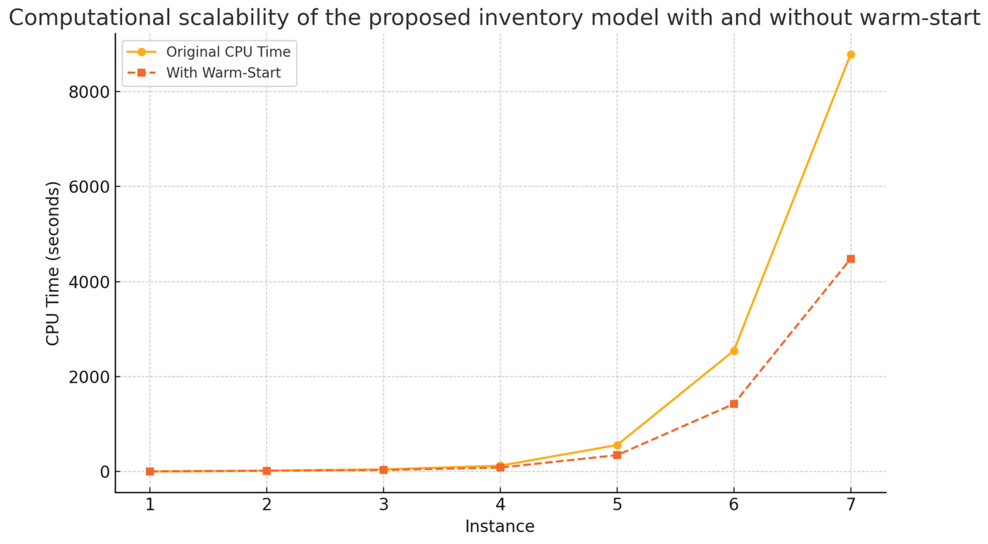
Table 1.
Literature Review.
| Reference | Objective of the study | Model | Solution procedure |
|---|---|---|---|
| Björk (2009) |
Develop an analytical solution to an EOQ problem with demand uncertainty. | FNLO1 | Analytical solution. |
| Chung et al., (2018) | Incorporate the concepts of two levels of commercial credit (retail and customers). | NLO2 | Analytical solution. |
| Thorsen & Yao (2017) | Develop a robust optimization model with uncertainty in demand and lead time. | LP3 | Benders decomposition algorithm. |
| Yang et al., (2017) | Propose a multi-item inventory classification and control optimization model. | MILP4 | MILP (Branch and Bound algorithm). |
| Shi et al., (2022) | Formulate and apply an inventory optimization model. | MILP | MILP (Branch and Bound algorithm). |
| Zhang (2010) | Develop a multi-period, newsboy-type model with budget constraints and quantity discounts. | MINLP5 | Lagrangian relaxation heuristic. |
| Sicilia et al., (2022) | Develop a multi-product, single-period, stochastic demand and power pattern model in the inventory cycle. | SNLP6 | Lagrangian relaxation heuristic. |
| Maiti & Maiti (2007) | Develop a multi-product inventory model, in two warehouses, with fuzzy stochastic demand and costs. | NLFSP7 | Genetic region reduction algorithm (RRGA). |
| Taleizadeh et al., (2011) | Build a multi-restrictive joint product model for purchasing high-priced raw materials. | INLFP8 | Hybrid harmony search method, fuzzy and approximate simulation. |
| Saracoglu et al., (2014) | Formulate a reorder point model focused on multi-product management, under budget, storage, and shelf-life restrictions. | ILP9 | Genetic algorithm (GA). |
| Hammami et al., (2014) | Formulate an inventory model with supplier selection, multiple warehouses, quantity discounts, and uncertainty in the purchasing process. | MISP10 | MILP (Branch and Bound algorithm). |
| Abginehchi et al., (2013) | Develop a mathematical model that incorporates multiple suppliers, with a single product and retailer under probabilistic demand. | SO11 | Sequential quadratic programming algorithm (SQP). |
| Güder & Zydiak (2000) | Solving a multi-joint inventory problem with storage limitations, using a heuristic procedure. | NLO12 | Fixed cycle heuristic. |
| Đorđević et al., (2017) | Solving the storage-constrained EOQ model using a metaheuristic approach. | NLO | Local Search Heuristic and Variable Neighborhood Metaheuristic. |
| Jana & Das (2017) | Study a two-warehouse inventory model with multiple discounted items nested in unit cost and inventory costs over a fixed-cost period. | MINLP | Multi-objective genetic algorithm with variable population (MOGAVP). |
| Kumar & Mahapatra (2021) |
Plantear un modelo de minimización de costos asociado a la gestión de inventarios de múltiples artículos, con múltiples proveedores y múltiples almacenes. | NLO | Metaheurística de optimización de lluvia (ROA). |
Source: The authors.
Table 2.
Hardware specifications.
| Processor | AMD RYZEN 5, 2,8 Ghz. |
|---|---|
| RAM | 24 Gb |
| Operating System | 64 bits. Windows 11 |
| Optimization Software | LINGO 19 |
| Integer optimality tolerances | 1*10-6 (absolute), 8*10-6 (relative) |
| Linear optimality tolerances | 1*10-7 (absolute). |
Source: The authors.
Table 5.
Results of instances of the computational tests.
| Model characterization | Instances | ||||||
|---|---|---|---|---|---|---|---|
| Indicators | 1 | 2 | 3 | 4 | 5 | 6 | 7 |
| Integer Variables | 1.937 | 4.199 | 17.376 | 43.460 | 124.080 | 290.394 | 571.480 |
| Binary Variables | 40 | 72 | 243 | 432 | 1.080 | 1.944 | 3.024 |
| Total Variables | 1.977 | 4.271 | 17.619 | 43.892 | 125.160 | 292.338 | 574.504 |
| Total Restrictions | 1.881 | 4.141 | 14.536 | 24.778 | 63.127 | 111.358 | 175.681 |
| CPU time (s) | 4 | 22 | 47 | 126 | 560 | 2.546 | 8.782 |
| Warm start - CPU Time Reduction (%)* | 0% | 15% | 25% | 32% | 38% | 44% | 49% |
| Generator Memory Used (kB) | 663 | 1.400 | 5.388 | 9.918 | 37.109 | 74.338 | 168.629 |
*Note: The percentages indicate typical CPU time reductions achieved using warm-start heuristics and preprocessing strategies. Source: The authors.
Disclaimer/Publisher’s Note: The statements, opinions and data contained in all publications are solely those of the individual author(s) and contributor(s) and not of MDPI and/or the editor(s). MDPI and/or the editor(s) disclaim responsibility for any injury to people or property resulting from any ideas, methods, instructions or products referred to in the content. |
© 2025 by the authors. Licensee MDPI, Basel, Switzerland. This article is an open access article distributed under the terms and conditions of the Creative Commons Attribution (CC BY) license (http://creativecommons.org/licenses/by/4.0/).
Copyright: This open access article is published under a Creative Commons CC BY 4.0 license, which permit the free download, distribution, and reuse, provided that the author and preprint are cited in any reuse.


