
Submitted:
14 May 2025
Posted:
14 May 2025
You are already at the latest version
Abstract
Power smoothing for renewable energy resources is receiving increasing attention. One widely used resource is the grid-tied photovoltaic (PV) system. Solar energy production typically follows a Gaussian bell curve, with peaks at midday; however, climate varia-tions can significantly alter this pattern. This paper aims to smooth the power supplied to the grid by the PV system. The proposed controller manages the charge and discharge processes of the Energy Storage System (ESS) to ensure a smooth Gaussian bell curve out-put. It adjusts the parameters of this curve to closely match the generated energy, absorb-ing or supplying fluctuations to maintain the desired profile. This system aims also to provide accurate predictions of the power that should be supplied to the grid by the PV system, based on the capabilities of the ESS and the overall system performance. Although experimental results were not included in this analysis, the system was implemented in SIMULINK using real-world data. It utilizes a hybrid ESS comprising a Vanadium Redox Battery (VRB) and Supercapacitors (SC). The design and operation of the controller, in-cluding curve tuning and ESS charge‒discharge management, are detailed. The simula-tion results demonstrate excellent performance and are thoroughly discussed.
Keywords:
energy storage system (ESS)
; electrical power system
; grid-tied PV
; vanadium redox battery (VRB)
; supercapacitors (SC)
; gaussian distribution
1. Introduction
The exponential growth of renewable energy resources has introduced rapid fluctuations in the power they generate, significantly impacting grid stability. The increasing contribution of renewable energy sources to the grid is noteworthy. Electricity generated by these resources is subject to natural variability; for instance, in PV systems, output fluctuates based on factors such as cloud cover, temperature, and solar irradiation. ESS are widely used to mitigate the intermittency of renewable energy sources, especially in grid-connected systems [1]. Their primary function is to smooth power output through peak-cutting and valley-filling [2]. Batteries are commonly used as ESS, but reducing their size presents both technical and financial challenges [3]. An effective controller for power smoothing is essential to address these challenges, especially under unpredictable weather conditions.
Various methods have been developed to control the charging and discharging processes, ensuring predictable and stable delivery of power from renewable resources. Techniques such as low-pass filters, moving averages [4,5], fuzzy logic [6], neural network-based predictive systems [7], and deep reinforcement learning [8], have been explored. This paper proposes a novel method for fine-tuning the Gaussian bell curve to provide a robust solution. The proposed method functions as a dynamic filtering mechanism throughout the day and adjusts in real time based on key ESS parameters, such as the State of Charge (SOC). Additionally, the controller actively manages the ESS to prevent overcharging or excessive discharging.
It should be noted that previous studies have utilized Gaussian filters to smooth generate energy [9]. However, this paper adopts a different approach by focusing on the Gaussian bell curve, which represents the Gaussian distribution. Additionally, a study in [10] highlights the Gaussian distribution of PV and wind energy, which aligns closely with the concept presented in this paper.
While earlier smoothing methods sought to predict the next set of data without considering the broader context, this paper examines the behavior of PV-generated energy across the entire day. It provides a comprehensive perspective on predicting daily energy production by analyzing variations at different hours. The tuning process further enhances the reliability of the proposed approach. The method introduced in this paper is both simple and effective. Although it aligns with the objectives of previous research, it differs significantly in its approach by analyzing the energy output of a PV system over an entire day and establishing a reference framework.
This paper adopts a comprehensive perspective to present an effective solution, as demonstrated by the results. The chosen system is detailed in Section II, while the collected PV data from two sources is discussed in Section III. The process of deriving and tuning the Gaussian bell curve for parameter adjustments is outlined in Section IV. Section V describes the controller developed for the entire system, and the results are presented and analyzed in Section VI. Section VII provides a comparison to illustrate the achieved curves in relation to the theoretically fitted curves.
2. System Description
The proposed network comprises the electricity grid, renewable energy resources, and an energy storage system (ESS). The ESS is designed to smooth the energy supplied to the grid by the renewable energy resource, specifically the PV solar system. It is a hybrid system consisting of a vanadium redox battery (VRB) and super-capacitors (SC). Energy smoothing is achieved by absorbing sudden increases in energy generated by the PV system and supplying energy to the grid to counteract sudden decreases caused by the PV system. This system was previously utilized and discussed in [11].
Figure 1 presents the block diagram of the system. The VRB used is the E22 Energy Storage Solutions 400 kWh model, designed for four-hours operation. The SC system is the MAXWELL TECHNOLOGIES BMOD0165 P048 BXX model, configured with 14 cells in series at 660 V DC and 35 sets in parallel, resulting in a total of 14x35 (490 cells) and a capacity of 26 kVA. The equivalent models implemented in Simulink are described in [11]. The hybrid system VRB and SC are often utilized as a hybrid storage solution. The batteries offer high energy density, which is suitable for long-term charging and discharging, while the SC high power density, enabling rapid response times. This paper introduces modifications focused on the controller. The VRB offers numerous advantages as an ESS [7], with an effective efficiency range in the SOC window of 20-85%. Incorporating SC into the hybrid system enhances its ability to eliminate fluctuations in renewable energy resources, making it one of the most effective solutions [7,13].
3. PV Data
The data tested in this study was obtained from two sources. The first dataset was collected from a 30 MW PV plant in Malaysia between 30/June/21 and 8/July/21. It was gathered using a Fluke meter connected to the output of a 2 MW plant inverter, as described in [11]. The collected power data is shown in Figure 2. The second dataset was sourced from a project conducted by UK Power Networks, with data recorded at 1-minute intervals during the summer of 2014 [14]. A portion of this dataset is presented in Figure 3(a). The data shown in Figure 3 (a) represents the output of UK Power Networks, scaled by a factor of 660 to align with the output collected in Malaysia. The original data collected over two days, as shown in [11], is displayed in Figure 3 (b). This figure highlights the difference between a sunny and a cloudy day.
4. Gaussian Smoothing
The characteristic power generated by a PV system during the day generally resembles a bell curve, similar to a Gaussian distribution. The total power supplied throughout the day can be smoothed to follow a Gaussian function 13], defined as:
where (a) is the height of the curve’s peak, (b) is the position of the center of the peak, and (c) controls the width of the “bell”, as shown in Figure 4. The parameters in Equation (1) can be adjusted or tuned to achieve a curve that closely matches the generated power. For simplicity, (b) (the position of the center of the peak) can be assumed constant, as it typically corresponds to midday (noon). Meanwhile, (a) and (c) can be tuned to achieve the desired curve. The times of sunset and sunrise vary according to seasons, latitude, and longitude. This affects (a) and (c) in the bell curve, with (a) corresponding to radiation and (c) depending on location and time of year. As illustrated in Figure 4, altering (c) changes the width of the bell curve, while adjusting (a) modifies the height of the peak. Changes to (c) (the width) significantly affect the error during periods of low radiation, mathematically corresponding to times far from (b). Conversely, adjustments to (a) (the peak height) have a substantial effect on the error during periods of high radiation, mathematically closer to (b). From these observations, the error can be used to tune (a) and (c) proportionally to the time of day relative to (b) for (a), and inversely for (c). To simplify, the change factor (Cfact) in (a) and (c) due to the error can be derived as:
where Time is the time in minutes from midnight, b is the time in minutes corresponding to the peak radiation (as defined in Equ. (1)). The error is calculated as the difference between the total power (or discrete current values, assuming the voltage remains nearly constant) and the total area under the Gaussian bell curve. The control system adjusts (a) and (c) by incrementally adding or subtracting small values to minimize this error. Another important factor to consider is the SOC of the battery. Adjustments to (a) and (c) must ensure that the SOC remains around 0.5, as this minimizes the adverse effects of a fully charged or completely discharged battery. The updated values of (a) and (c) can be derived as:
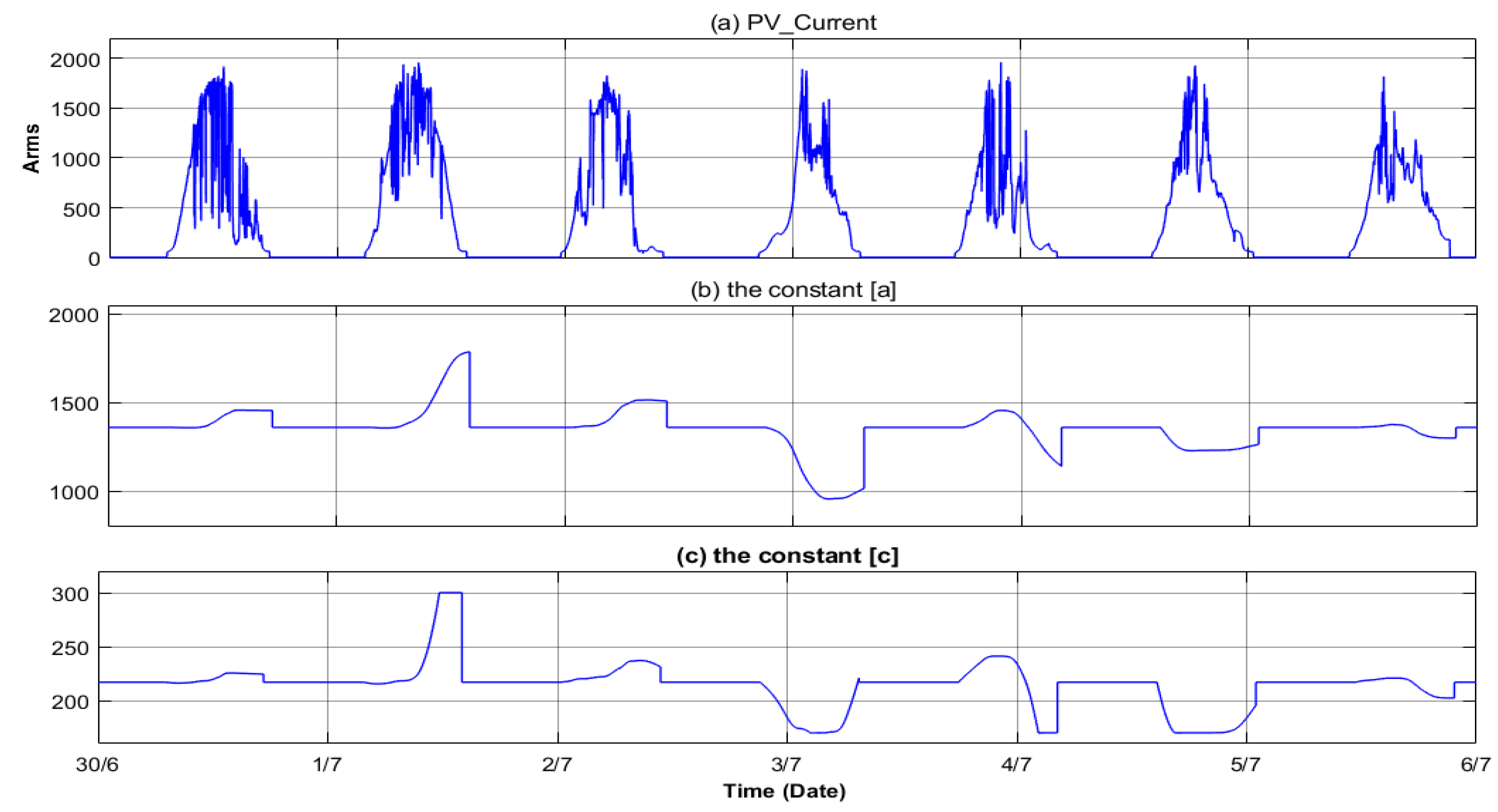
where Ppv is the power generated by the PV system from the start of the day, AreaBell represents points on the generated bell curve, and k is a factor used to minimize the step change -(k=0.1)-. The values (a0) and (c0) are the averages of their respective variables over the last several days. Each day starts with the assumption that (a= a0) and (c=c0), with the tuning process starting at 5:00 am, as the power summation before that time is negligible.
The previous equations provide a reliable approximation of the smoothed average power of the PV system. However, in practical applications, two additional factors must be considered to make the smoothing process more effective. Firstly, the power generated in the morning does not follow a bell curve. Instead, it remains near zero before increasing rapidly with the onset of sunshine. A similar phenomenon occurs at sunset, where the power drops sharply. This problem was addressed by ensuring zero power is assumed outside the sunshine period, defined as the hours of 5:00–20:00. Secondly, the changes in PV-generated power can exhibit significant, abrupt variations, which could drive the SOC to its limits (either fully charged or fully discharged). To mitigate this, approximately ±10% of the total power was added to the bell curve. Thus, Equation (1) becomes:
The expression of is as follows:
where Pcrt=0.05*Pmax (Pmax: maximum power generated by the PV system), this level can be maintained until 15:00 . After this time, it can be increased by up to 10%, so Pcrt=0.1*Pmax if the SOC deviates significantly from 50%. This adjustment helps the battery maintain approximately half of its charge, ensuring it begins the next day with an effective charge level. It is important to note that if the battery is intended to serve as a power source during peak consumption hours, SOCcorrection should be used (SOC-0.8) Pcrt during the final hours of the day to keep the battery near a 50% charge level. Additionally, the early hours of the day can be used to charge the battery 50% in such scenarios.
5. Control Process
The implemented controller is designed to reduce imitation fluctuations in PV-generated power by providing an expected average power as closely aligned as possible with the actual generated power. This approach enables the Energy Storage System (ESS) to absorb surplus power and supply additional power to smooth out fluctuations, thereby maintaining network stability. Achieving an accurate estimation of the PV average generated power minimizes the size and cost of the ESS required for smoothing.
The controller performs three main functions: generating the optimal expected average power (based on the methodology described in the previous section), managing the charging and discharging of the battery to achieve power smoothing, and controlling the selection of charging and discharging between the VRB and SC to prevent overcharging or excessive discharging.
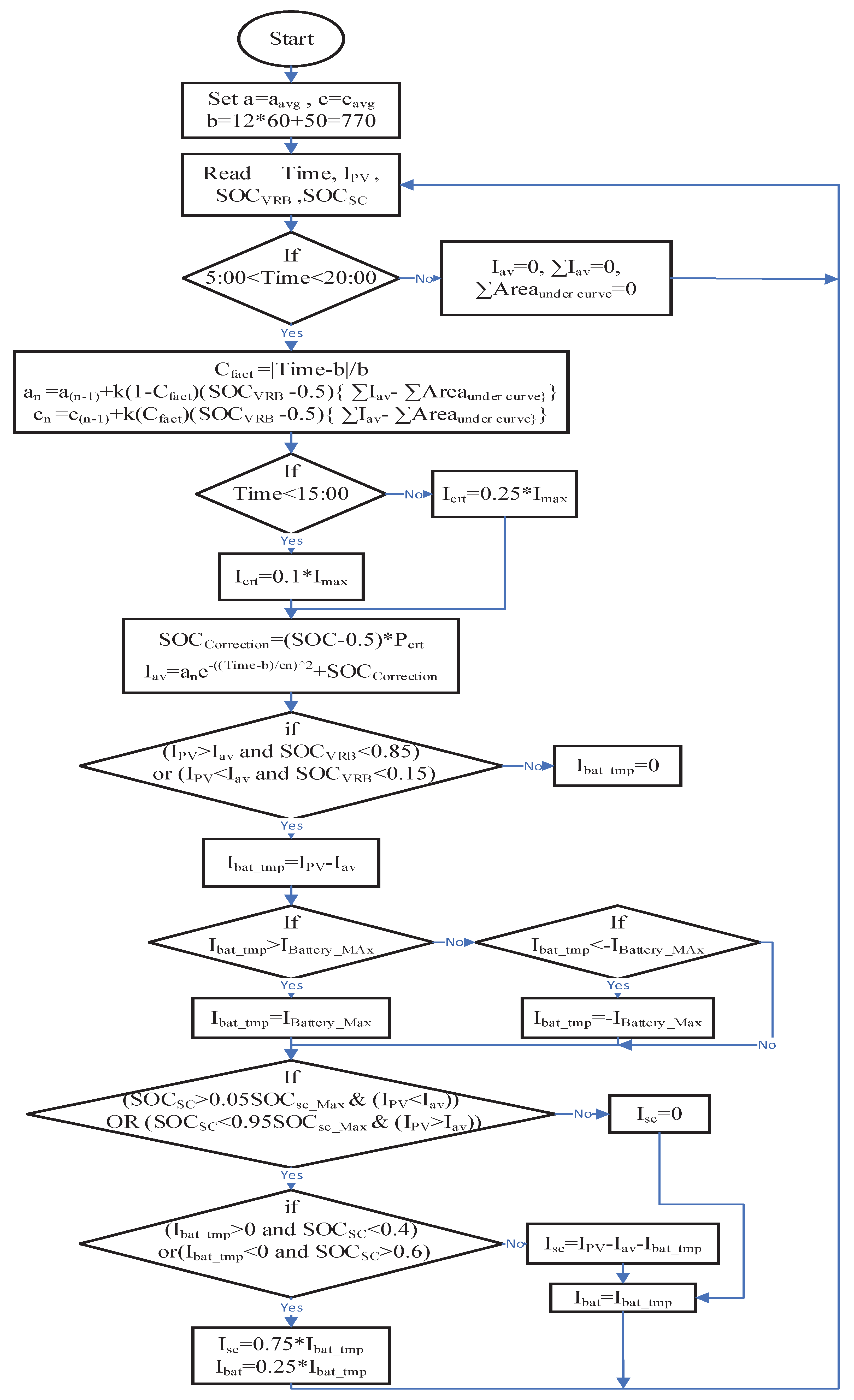
This functionality is implemented by monitoring the PV-generated current and the State of Charge (SOC) of the VRB and SC. These parameters determine the current that needs to be absorbed or generated by the VRB and SC, as shown in the flowchart in Figure 5. The system was simulated using SIMULINK by incorporating the collected data from Section II as a PV current source. To optimize simulation efficiency, an average inverter model was used. The SOC of the SC was calculated as described in [11].
The relationship between the charging and discharging processes of the VRB and the SC is illustrated in the flowchart shown in Figure 5. When the state of charge of the VRB (SOCVRB) is low and the state of charge of the SC (SOCSC) is high, the controller will prioritize charging the VRB to over 50% during the charging process, with the remaining charge directed to the SC. Conversely, during the discharging process, the controller will discharge the SC more than the VRB. This pattern reverses when the states of charge are swapped.
7. Simulation Results
The new controller, outlined in the flowchart in , was implemented within the system shown in Figure 6. This controller regulates the charging process for both the VRB and the SC. The parameters (a), (b), and (c) in Figure 4 were estimated based on the average of previous test data. The system stores the average values of parameters (a), and (c) from the last ten days, while (b) is kept constant. Two cases of collected data are shown in and. The simulation was performed using MATLAB Simulink, adhering to the methods described in Section II to ensure the results closely reflect real-world applications. The simulation utilized averaged bidirectional inverters for both the VRB and SC, functioning as a three-phase current source to replicate the measured current observed in practice.
Figure 5.
Control process flowchart.
These assumptions were made to expedite the simulation process. While minor losses and transient cases may occur, they are not expected to significantly impact the overall results. The simulation results for the PV data collected from Malaysia, as shown in Figure 2, were simulated and displayed in Figure 7. The figure illustrates: the original current generated by the PV system, the current absorbed or supplied by the VRB, the current absorbed or supplied by the SC, the current supplied to the system, which exhibits an almost Gaussian bell shape, and the SOC of both the VRB and SC. The results illustrate a smooth output closely resembling a Gaussian bell curve. The controller successfully maintains the SOC of the VRB around 0.5, which aligns with the recommended range in 15], between [20-85%]. It is evident that the VRB is charged and discharged sequentially to smooth the power supplied to the grid. Guided by the reference signal generated by the controller, the dissipated power aligns with the expected curve, enhancing grid stability. Figure 8 displays the controller’s output for data collected by UK Power Networks, as shown in . This figure shows the original current generated by the PV system, the current associated with the VRB and SC, the current supplied to the grid, and the SOC of both the VRB and SC. The results are similar to those presented in 11; however, on 23/6/2014, the battery reached full charge. Figure 9 focuses on data from 30th June in Malaysia, providing detailed insights into how the ESS absorbed the current that exceeded the expected curve. The ESS effectively supplied sufficient current to meet the proposed curve. Additionally, Figure 9 highlights instances of unsmoothing caused by the full discharge of the SC and the limitations of the VRB in filling the supply gap. The tuning parameters (a,c) are displayed in Figure 10. Each day starts with the average values from the previous 10 days, as previously discussed. Adjustments are made throughout the day according to the flowchart in Figure 5.
Figure 6.
Simulink block diagram for the system.
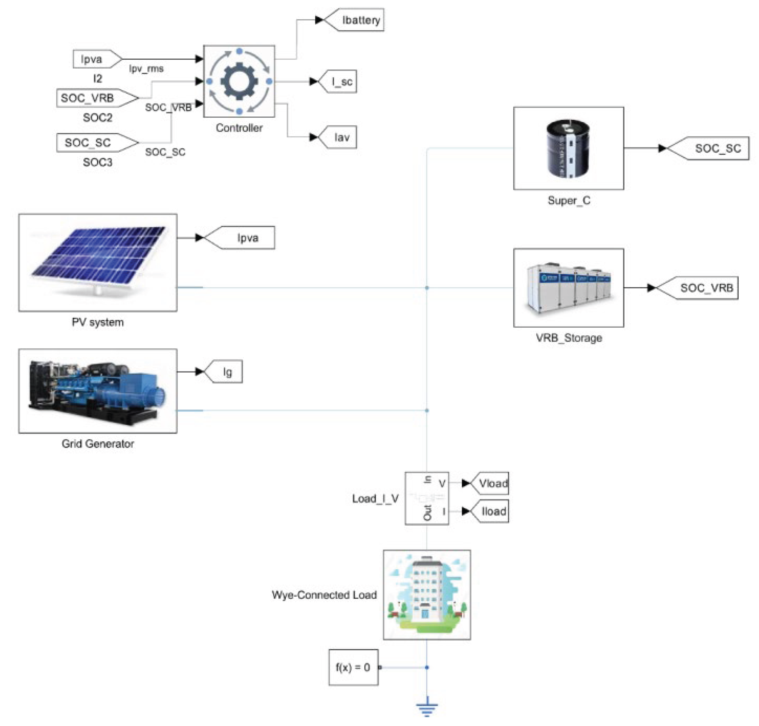
Figure 7.
Simulation results for the collected data in (30/6-8/7) from Malaysia: (a) The Ipv is the PV-generated current, (b) IBatt is the current absorbed or supplied by the VRB, (c) Isc is the current absorbed or supplied by the SC, (d) the current supplied to the grid, (e) the SOCBatt of the VRB battery, and (f) the SOCsc of the capacitor SC.
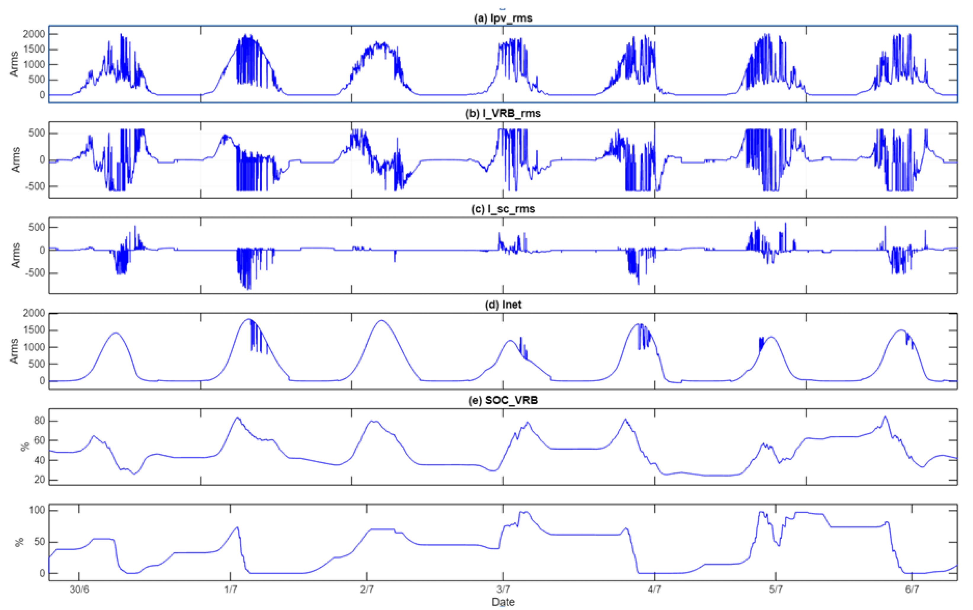
Figure 8.
Simulation results for the collected data in (20/6-25/6) from the UK: (a) the Ipv represents the PV-generated current, (b) IBatt represents the current absorbed or supplied by the VRB, (c) Isc represents the current absorbed or supplied by the SC, (d) the current supplied to the grid, (e) the SOCBatt of the VRB battery, and (f) the SOCsc of the capacitor SC.
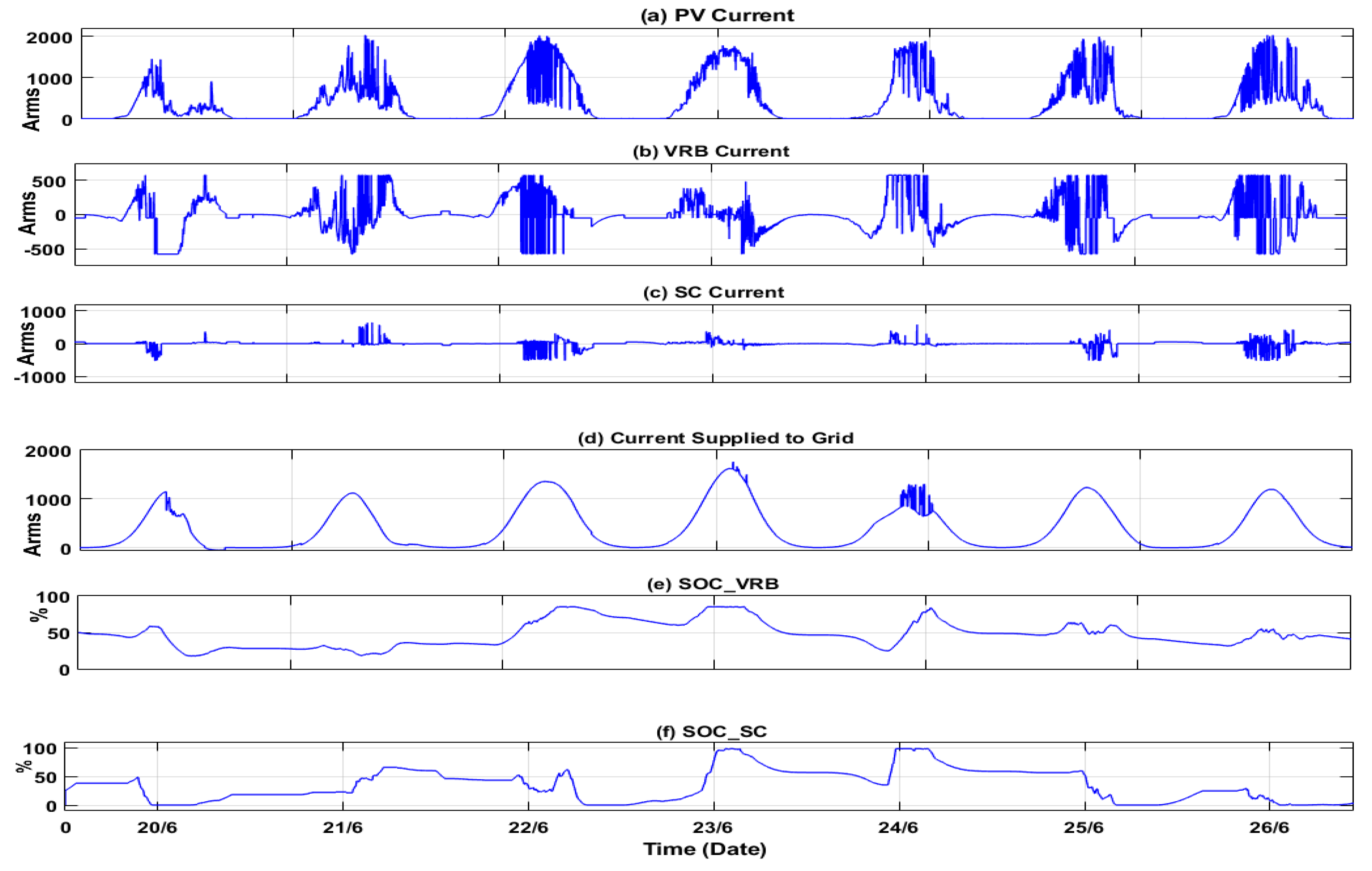
Figure 9.
Focused on the charging and discharging process that caused smoothing. (a) The data collected in (29/6) from Malaysia and the current supplied to the grid. (b) VRB and SC charging and discharging.
Figure 9.
Focused on the charging and discharging process that caused smoothing. (a) The data collected in (29/6) from Malaysia and the current supplied to the grid. (b) VRB and SC charging and discharging.
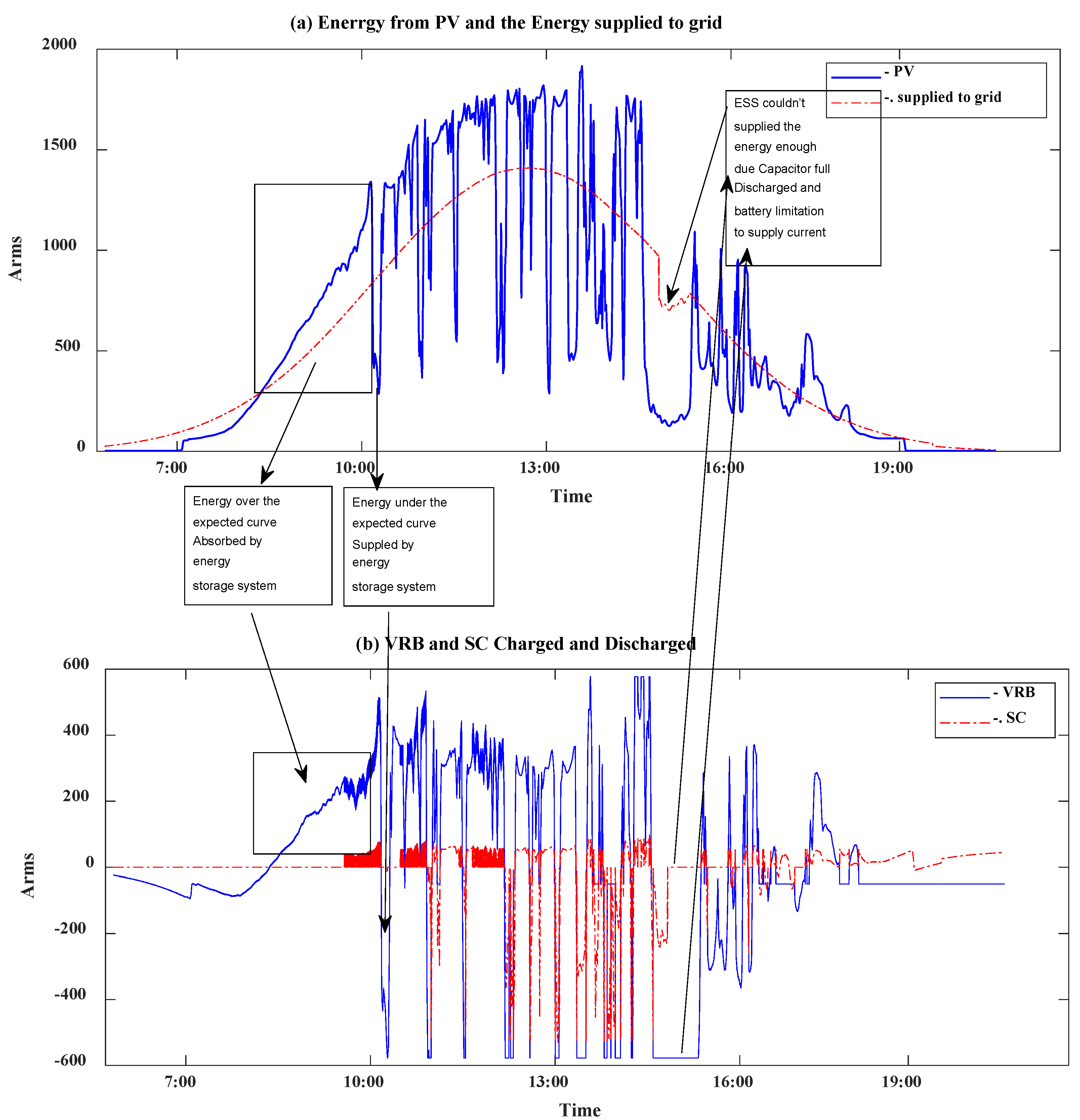
Figure 10.
Simulation results for the constants (a and c) for smoothing the collected data (1/7-6/7) from Malaysia.
Figure 10.
Simulation results for the constants (a and c) for smoothing the collected data (1/7-6/7) from Malaysia.
8. Comparison of Results
The parameters (a), (b), and (c) depend on statistical and probability fitting, which is one of the methods that can be used to determine them, along with other methods referenced in [16] and [17]. In this research, the goal is to enable real-time expectations, which is the primary contribution of this paper.
This method relies on statistical analysis, with the primary objective of generating curves that smoothly represent the power output from the (PV) system. The challenge of these curves is to balance the power or currents above them with those below. In an ESS, this means that charging should be nearly equal to discharging. Currently, there is no ideal curve that can serve as a reference for comparison. The goal of achieving equilibrium between charging and discharging can be easily verified by monitoring the (SOC). Maintaining the SOC around 50% indicates that charging and discharge are nearly equal.
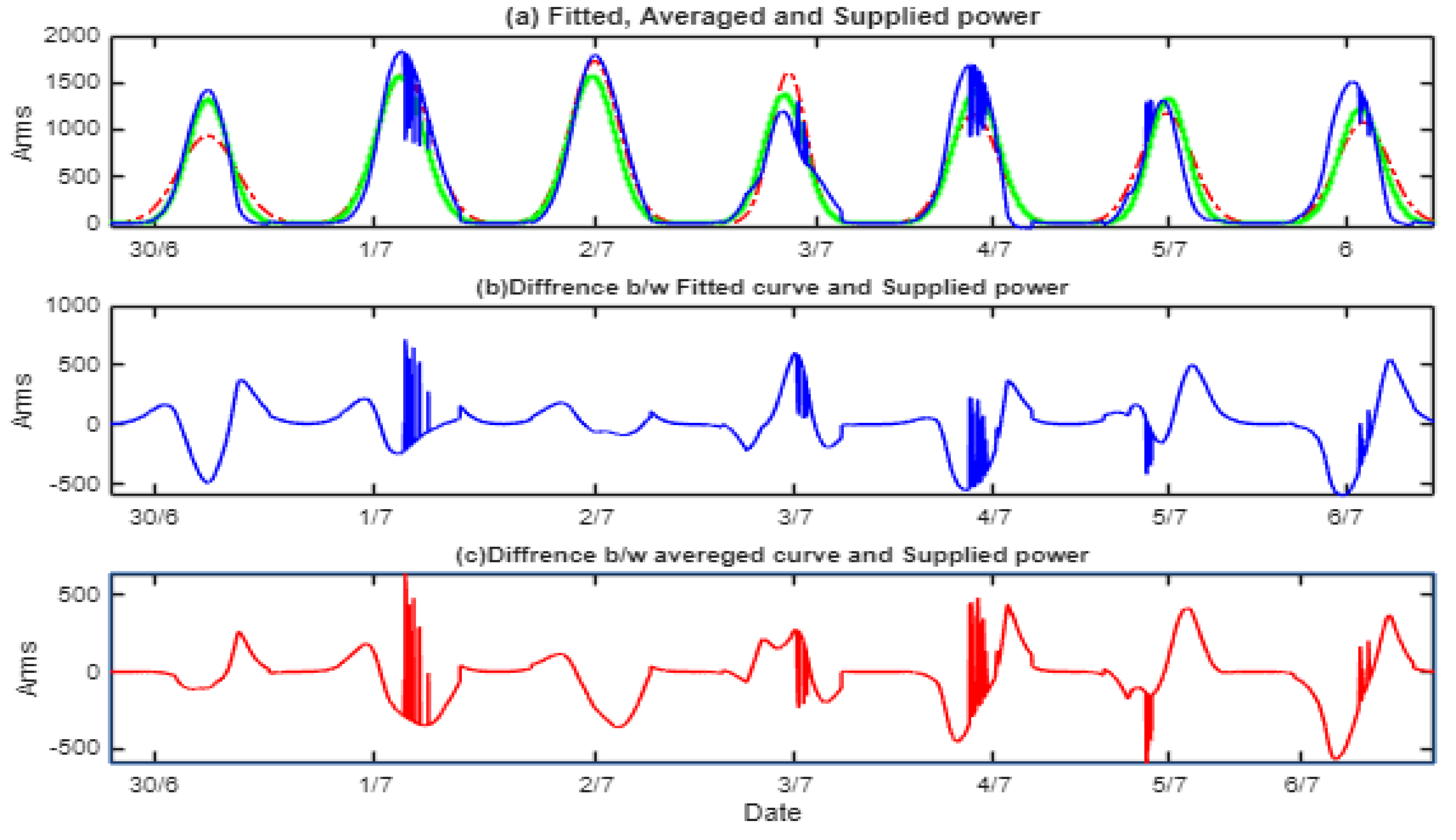
A comparison with a known reference enhances confidence. The data presented in Figure 2 was fitted using Gaussian fitting in MATLAB, referred to as the reference curve. can be performed after obtaining the data, serving as a reference point. Additionally, the calculated averages of (a) and (c) were used in Simulink to generate a Gaussian curve, termed the reference curve. The current supplied to the grid, as shown in the real-time simulation of part d in Figure 7, represents the achieved curve.
Figure 11 illustrates the comparison. In part A, it shows the curve generated by MATLAB through fitting, the generated curve using the averaged parameters for a specific date, and the power supplied to the grid using this system in Simulink. It is evident that the three curves exhibit significant similarity. The differences between the achieved curve and the ideal reference curve in certain areas are attributed to smoothing or minor fluctuations caused by full charging or discharging, as previously shown in Figure 10.
9. Conclusions
The smooth Gaussian bell shape of the power delivered to the grid was successfully achieved. The controller dynamically adjusted the Gaussian bell parameters (a,c) to generate a reference signal that minimized the likelihood of the battery becoming fully charged or completely discharged. The SOC was maintained around 50%, optimizing battery efficiency and prolonging its lifespan. The hybrid system effectively absorbed current fluctuations. Although the system was simulated and neglected some transient cases, it utilized real instrument parameters (VRB and SC) and real collected data. Furthermore, the simulation was conducted using MATLAB Simulink, a highly trusted simulation software. The Gaussian tuning method provided a highly effective solution for power smoothing by optimally controlling the energy storage system in conjunction with the PV plant.
In addition, the approach of tuning the Gaussian bell shape using parameters has the potential to address a wide range of challenges in other applications that rely on the natural Gaussian curve.
References
- Dasa, U.; Teya, K.; Seyedmahmoudiana, M.; Mekhilefb, S.; Idrisc, M.; Deventerc, W.; Horanc, B.; Stojcevski, A. Forecasting of hotovoltaic power generation and model optimization: A review. Renewable and Sustainable Energy Reviews 2018, 81, 912–928. [Google Scholar] [CrossRef]
- Li, J.; Hu, D.; Mu, G.; Wang, S.; Zhang, Z.; Zhang, X.; Lv, X.; Li, D.; Wang, J. Optimal control strategy for large-scale VRB energy storage auxiliary power system in peak shaving. Electrical Power and Energy Systems 2020, 120. [Google Scholar] [CrossRef]
- Laajimi, M.; Go, Y. Energy storage system design for large-scale so- lar PV in Malaysia: Techno-economic analysis. Renewables: Wind, Water, and Solar 2021, 8.
- Syed, M.; Abdalla, A.; Al-Hamdi, A.; Khalid, M. Double Moving Aver- age Methodology for Smoothing of Solar Power Fluctuations with Bat- tery Energy Storage. 2020 International Conference on Smart Grids and Energy Systems (SGES), 23-26 November 2020, pp 291-296.
- Atif; Khalid, M. Saviztky–Golay Filtering for Solar Power Smoothing and Ramp Rate Reduction Based on Controlled Battery Energy Storage. IEEE Access 2020, 8, 33806–33817. [Google Scholar] [CrossRef]
- XLi; Li, N.; Jia, X.; Hui, D. Fuzzy logic based smoothing control of wind/PV generation output fluctuations with battery energy stor- age system. 2011 International Conference on Electrical Machines and Systems, Beijing, China, 2011, pp. 1-5.
- Etxeberria; Vechiu, I.; Baudoin, S.; Camblong, H.; Kreckelbergh, S. Control of a Vanadium Redox Battery and supercapacitor using a Three-Level Neutral Point Clamped converter. Journal of Power Sources 2014, 248, 1170–1176. [Google Scholar] [CrossRef]
- Kolodziejczyk, W.; Zoltowska, I.; Cichosz, P. Real-time energy purchase optimization for a storage-integrated photovoltaic system by deep re- inforcement learning. Control Engineering Practice 2021, 106, 104598. [Google Scholar] [CrossRef]
- Desta; Courbin, P.; Sciandra, V. Gaussian-Based Smoothing of Wind and Solar Power Productions Using Batteries. International Journal of Mechanical Engineering and Robotics Research 2017, 6, 154–159. [Google Scholar] [CrossRef]
- Addisua; Georgeb, L.; Courbina, P.; Sciandra, V. Smoothing of re- newable energy generation using Gaussian-based method with power constraints. 9th International Conference on Sustainability in Energy and Buildings, Chania, Crete, Greece, 5-7 July 2017.
- Alyan, Ahmad and Abd Rahim, Prof. Dr. Nasrudin and Selvaraj, Jeyraj, Energy Storage System Sizing for a Grid-Tied Pv System: Case Study in Malaysia. Available at SSRN: https://ssrn.com/abstract=4968969 or http://dx.doi.org/10.2139/ssrn.4968969. [CrossRef]
- https://data.london.gov.uk/dataset/photovoltaic–pv–solar-panel-energy-generation-data , “Photovoltaic (PV) Solar Panel Energy Generation data”, Data collected as part of the project run by UK Power Networks. Jul, 2024.
- Guo, H. A Simple Algorithm for Fitting a Gaussian Function [DSP Tips and Tricks]. IEEE Signal Processing Magazine 2011, 28, 134–137. [Google Scholar] [CrossRef]
- Ceraolo, M.; Lutzemberger, G.; Poli, D. State-Of-Charge Evaluation Of Supercapacitors. Journal of Energy Storage 2017, 11, 211–218. [Google Scholar] [CrossRef]
- Li, J.; Hu, D.; Mu, G.; Wang, S.; Zhang, Z.; Zhang, X.; Lv, X.; Li, D.; Wang, J. Optimal control strategy for large-scale VRB energy stor- age auxiliary power system in peak shaving. International Journal of Electrical Power & Energy Systems 2020, 120. [Google Scholar]
- Peña, V.; Jauch, M. Properties of the generalized inverse Gaussian with applications to Monte Carlo simulation and distribution function evaluation. Statistics & Probability Letters 2025, 220, 110359. [Google Scholar]
- Zhu, Y.; Yao, W. A conditional probability density function model for fatigue damage estimation in broadband non-Gaussian stochastic processes. International Journal of Fatigue 2025, 197, 108958. [Google Scholar] [CrossRef]
Figure 1.
The system block diagram.
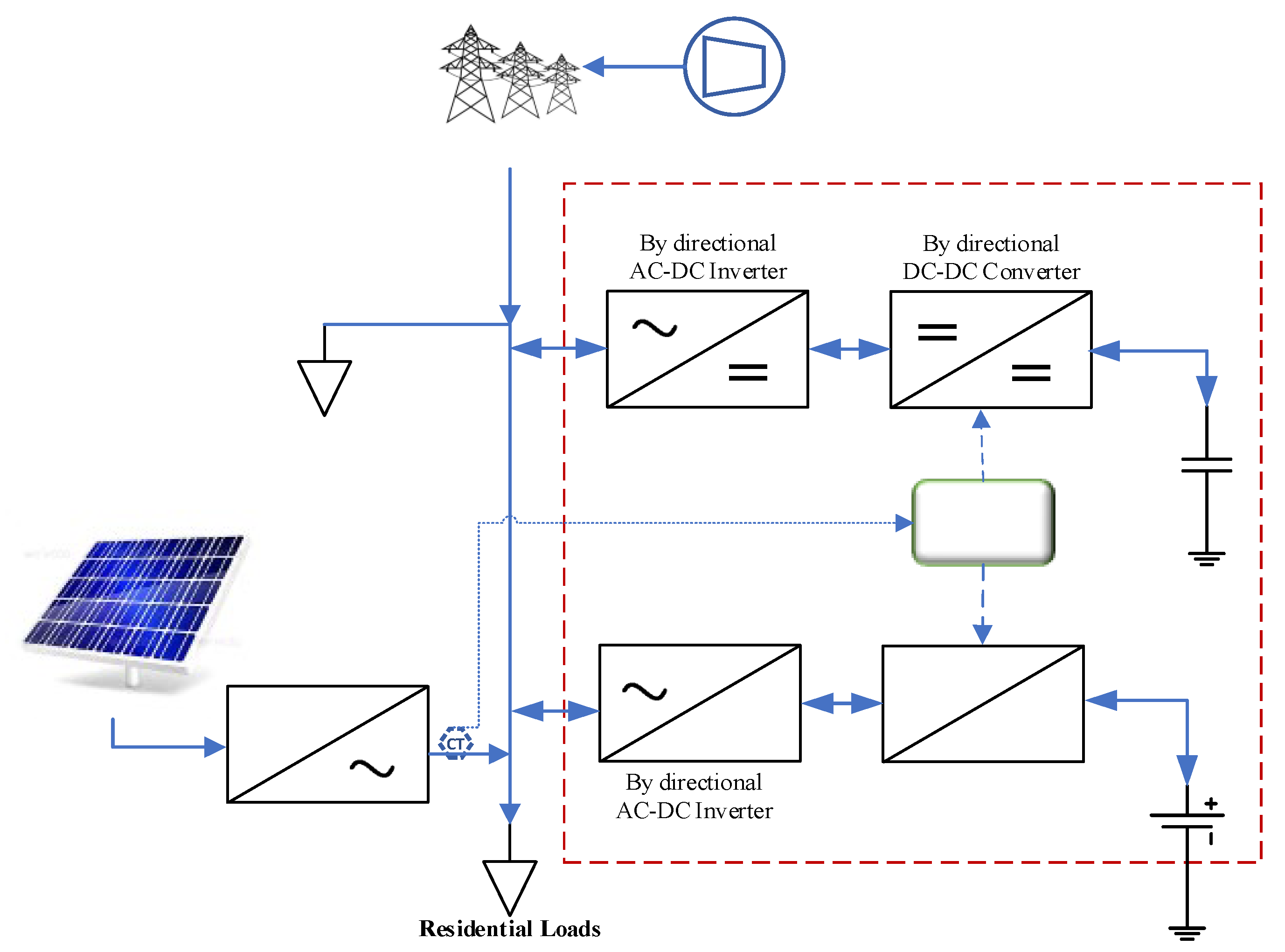
Figure 2.
PV output collected from 2 MW PVs in Malaysia between 30/June/21 and 8/July/21.
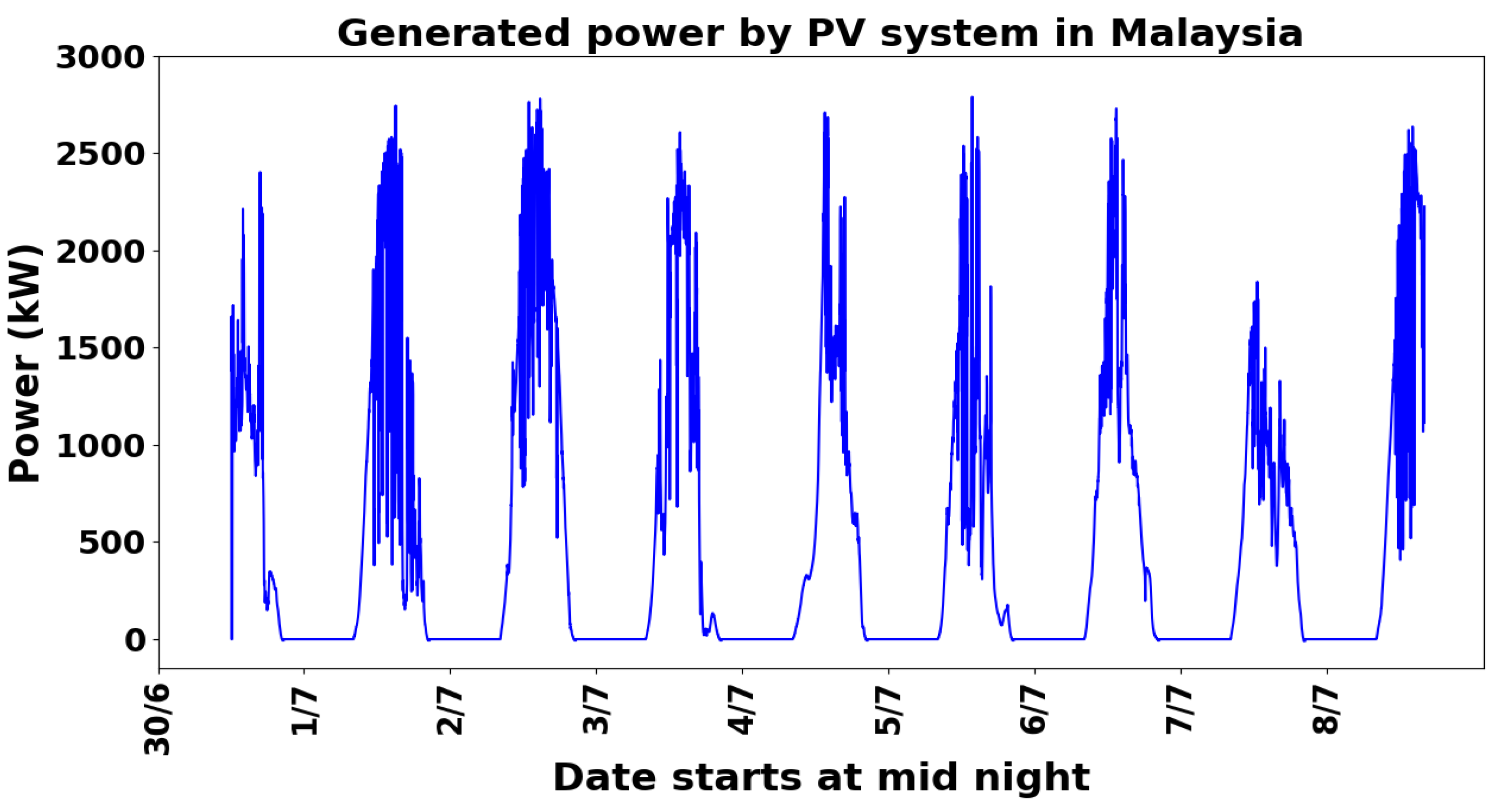
Figure 3.
(a) PV output collected from UK Power Networks 30/June/14–10/July/14. (b) PV output power at Maple Drive East collected from UK Power Networks – clear sunny day vs. scattered cloudy day – as in 11].
Figure 3.
(a) PV output collected from UK Power Networks 30/June/14–10/July/14. (b) PV output power at Maple Drive East collected from UK Power Networks – clear sunny day vs. scattered cloudy day – as in 11].
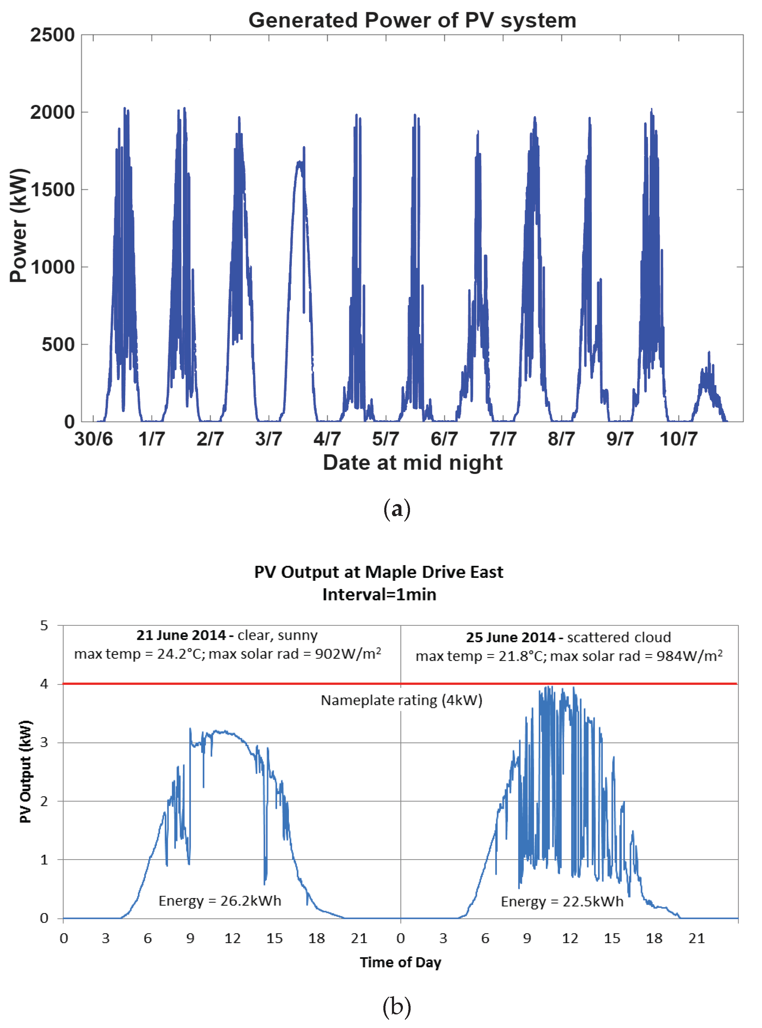
Figure 11.
Illustrates the comparison. Part A: the curve generated by MATLAB through fitting (red dash), the generated curve using the averaged parameters for a specific date (green), and the power supplied to the grid using this system in Simulink (blue). Part B: the error between the fitting and averaged curve, and Part C: the error between the fitting curve and the supplied power.
Disclaimer/Publisher’s Note: The statements, opinions and data contained in all publications are solely those of the individual author(s) and contributor(s) and not of MDPI and/or the editor(s). MDPI and/or the editor(s) disclaim responsibility for any injury to people or property resulting from any ideas, methods, instructions or products referred to in the content. |
© 2025 by the authors. Licensee MDPI, Basel, Switzerland. This article is an open access article distributed under the terms and conditions of the Creative Commons Attribution (CC BY) license (http://creativecommons.org/licenses/by/4.0/).
Copyright: This open access article is published under a Creative Commons CC BY 4.0 license, which permit the free download, distribution, and reuse, provided that the author and preprint are cited in any reuse.


