
Submitted:
22 June 2025
Posted:
24 June 2025
You are already at the latest version
Abstract
Energy storage systems (ESS) have recently emerged as a prevalent solution for mitigating the variability of intermittent renewable energy sources. One of the primary challenges associated with ESS is their cost. This paper aims to explore methods for reducing the size of ESS without compromising performance. Data was collected from a grid-tied 2MW PV unit in Malaysia over several days, as many variables exhibit significant fluctuations from hour to hour due to solar irradiation. Python code was developed to analyze the effects of varying ESS sizes on power grid smoothing. Both high-power density devices and high-energy density devices were tested, and the impact of changing output period durations was investigated. The output should remain stable for no less than five minutes, which is the minimum acceptable timeframe. SIMULINK was utilized to simulate the recommended ESS size, employing a vanadium redox battery (VRB) as the high-energy density device and supercapacitors (SC) as the high-power density device.
Keywords:
energy storage system (ESS)
; electrical power system
; grid-tied PV
; vanadium redox battery (VRB)
; supercapacitors (SC)
1. Introduction
Malaysia’s average solar radiation remains consistent across various scenarios. However, climate change can affect solar performance and infrastructure during the daytime due to extreme temperatures and precipitation [1]. Solar systems, like other natural resources, are heavily influenced by weather and seasonal changes [2]. Large Scale Energy Systems (LESS) are more significantly impacted than Small Scale Energy Systems (SLES). In recent years, energy storage systems have been employed to address the intermittent nature of renewable energy resources, particularly when integrated with the power grid. These systems can be categorized into mechanical and electrochemical batteries [3], with the latter being the primary focus of this paper. The cost of implementing battery energy storage systems (BESS) remains the most significant challenge. The approach proposed in this paper aims to minimize the size of the BESS while maintaining the performance and efficiency of the LESS in managing intermittency.
Grid sizing of (ESS) is crucial in grid planning due to the high capital costs involved and their significant impact on grid stability and efficiency [4]. Various methodologies can be employed to determine ESS sizing, depending on the specific objectives. Optimization techniques, probabilistic approaches, analytical models, and data-driven methods can be complex, largely due to the unpredictable nature of weather changes. However, data analysis has the potential to yield effective solutions. Several factors influence ESS sizing for renewable resources, including system characteristics, costs, grid stability and reliability requirements, and environmental impacts. Batteries are the most popular high-energy-density devices, while flywheels and SCs are commonly utilized as high-power-density devices.
Many studies have attempted to address ESS sizing. For example, in [5], the optimal ESS size in a microgrid was calculated with a focus on cost. Reference [6] consecrated on automatic generation control based on finite ramp rate control of PV peak, especially looking at smoothing of that ramp. Other studies have approached sizing from different perspectives, such as [7] which aimed to solve the issue of peak demand. Additionally, studies like [8]. have explored the probability of determining ESS sizing, while the study in [9]. merged renewable sources sizing with ESS sizing. Reference [10] joined optimizing the sizing and power management. Previous studies primarily examine sizing from a financial perspective. This study, however, takes an electrical engineering viewpoint and is based on real data and instruments in a hybrid system VRB with SC, which offers numerous advantages [11]. It presents a case study based on data collected from tropical Malaysia. It took nine days as an example since tropical climates repeat themselves, posing a challenge in their fast changes throughout the day.
This topology illustrates the process of ESS sizing based on collected data. The flowcharts outline the steps, using a hybrid VRB and SC were taken as an example of ESS. The type of ESS determines the limitations in real-world applications, and reducing the ESS size without compromising energy efficiency or the objective of utilizing ESS with renewable resources presents a significant challenge. A straightforward method of control, employing filtering and effective averaging, supports size reduction alongside other more efficient control methods. However, the technique derived in Equ 20- used for averaging, can also be applied by other modern or advanced controllers.
A topology is developed based on testing real data taken from an actual plant of renewable source. A Python code reads this data and trains it to determine the minimum ESS size that satisfies smoothing over a certain period. The code takes into account the type of ESS and its limitations based on market availability after checking its advantages. Finally, the ESS with the proposed size is simulated using MATLAB Simulink to ensure success. A simple and effective control method was developed in MATLAB Simulink to ensure storage system efficiency for grid stability, which can be achieved by regulating the grid generator during the subsequent settlement period to an appropriate level, allowing the (ESS) to maintain power output despite fluctuations in (PV) generation.
2. System Analysis
The system of this project consists of five parts -as shown in Figure 1: a) PV solar energy system, which includes PV panels and inverters connected to the grid, b) The grid (Generator with droop controller), c) Energy storage system ESS (Vanadium Redox Battery VRB and supercapacitors), d) Converters (bidirectional DC-DC and AC-DC), e) The load (residential network).
2.1. Collected Data
The data collected for this case study came from a 30MW PV plant in Malaysia. However, the data was collected using a Fluke meter from a 2MW plant inverter. Significant variables from the output side of the three-phase inverter include current, voltage, and power. While voltage changes are limited, the current has wide fluctuations which result in power changes.
A Python program was used to read the power data; Figure 2 summarizes (a) the power generated by the PV system between 30/June and 8/July/21, (b) the increase in generated power on 3/Jul, and (c) the average power generated within an 8-hour period. The total power generated was 98.3MW, with an average power of 501.2kW, and an average power of 1.503MW/h over an effective 8-hour period each day. On 2/7/21, the maximum daily power generated was 16.0MW, while the minimum was 9.1MW.
During the peak power generation period of 2790.0 kW at 12:43 pm on 05/07/21, the maximum increase within a minute was = 1437.0 kW, at 11:49 am on 01/07/21, and the maximum decrease was 1350.0 kW, at 11:08 am on 01/07/21. Changes greater than 420kW did not exceed 1%. The maximum gap within six minutes was 2142.0kW at 3:25 on 01/07/21.
During the peak power generation period of 2790.0 kW at 12:43 pm on 05/07/21, the maximum increase within a minute was = 1437.0 kW, at 11:49 am on 01/07/21, and the maximum decrease was 1350.0 kW, at 11:08 am on 01/07/21. Changes greater than 420kW did not exceed 1%. The maximum gap within six minutes was 2142.0kW at 3:25 on 01/07/21.
2.2. Storage System
Batteries are versatile and widely used for electrical storage due to their high energy density, rapid response time, and scalability. Despite this, lithium-ion batteries are the most popular. However, the VRB offers several advantages when it comes to large-scale energy storage systems. VRB and SC are often used as hybrid storage systems.
2.2.1. Vanadium Redox Flow Batteries (VRFBs)
VRFBs (Vanadium Redox Flow Batteries) are a promising energy storage technology due to their design flexibility, low manufacturing costs, long lifespan, and recyclable electrolytes [12]. VRB batteries have a long service life, which means that their chemical aging process is relatively slow compared to alternative battery technologies. Figure 4 illustrates the VRB structure [15]. VRFB’s cell membrane undergoes oxidation and reduction reactions during charging and discharging:
Figure 5 illustrates the equivalent circuit model. In this model, a voltage source represents the stack voltage, a controlled current source represents the current source, and a fixed loss resistance represents the parasitic losses of the pumps. Based on Randles’ circuit, which describes battery electrochemical properties [15], the terms “Resistive” and “Reaction” indicate the electrolyte solution resistance and the charge transfer resistance, respectively. Figure 5 illustrates the equivalent circuit for the VRB battery [14].
State of charge (SOC) refers to the percentage of battery charge to its fully charged state [14,15]. It provides a direct indicator of state of energy (SOE) stored in a battery. When the SOC reaches its upper or lower limits, typically defined as 80% and 20%, respectively [8], the inverter considers battery lifetime and deterioration mitigation. Other references may extend this range to 10%-90% [9]. These limitations should match the size of the batteries.
The VRB model can be derived as [12], the Estack which determined the battery voltage can be estimated by:
where n: number of cells, R: Universal gas constant (8. 144 JK-1.mol-1), T: Ambient Temperature (K), F: Faraday’s number, Ecell(at 50% SOC) : the cell equilibrium potential =1.39V.
The average DC output voltage from a 3phase full-wave rectifier is given by:
The number of cells in the stack (n) can be calculated to achieve 660V as flows:
The constant can be calculated at 30o degree as:
The Estack model of Figure 5 can be derived in SIMULINK by using (n) from Equ. (5) and constant from Equ. (6) Estack can be found on Simulink is shown in Figure 6.
The SOC can be estimated by the SOC Estimator derived in [15] as flows:
where: c: constant, Tstep: simulation step time, Trate: Battery charge or discharge time, and Prate: Battery power. From Equ. (8) the SOC can be the results of the integrator of ∆SOC the Simulink SOC Estimator can be shown in Figure 7.
The Flow Pump model of the equivalent circuit of Figure 5 can be derived as [15], the electrolyte flow rate (Q) is:
where (Istack): the flow rate is directly proportional to Stack current and inversely proportional to SOC and (N): electrolyte capacity.
The Flow Pump current can be derived as:
The pump loss can be represented by a controlled current source (I_parasitic), a shunt resistance (R_parasitic), and a combined resistance of the pump internal resistance and the auxiliary control circuit resistance (13.889Ω) [16].
Therefore, the Flow Q estimator for VRB on Simulink is shown in Figure 8. Calculations of VRB parameters are based on an estimation of 15% internal losses and 6% parasitic losses. The cell stack output power should be [17]:
where: Pn is the rated power. The fixed losses are represented as a fixed resistance and the variable losses are represented as a controlled current source. The losses are as follows [17]:
where Pf : The parasitic losses, k: is a constant value, in [17] assumed to be 1.011. The losses measured in kw. The 250kWh product E22 Energy Storage Solutions Company produces can be considered a storage device. Its typical characteristic, as shown Table 1Error! Reference source not found., is its overload capability: 30% discharge within one hour when the SOC exceeds 60% and 25% charge for 45 minutes when the SOC exceeds 25%; this means that 30% should be supplied or absorbed in one hour.
where PBattary: the instantaneous power of the battery, Vrms: is the nominal grid voltage.
This value can be the current limitation of charging and discharging current for the constant c in Equ. (10) which depends on total power (250kw), sampling (5ms), and rate time (4 hours), constant c:
2.2.2. Super Capacitors (SC)
SCs are energy storage devices that can store and deliver energy more rapidly than batteries. By integrating SC into systems alongside batteries, transient energy peaks can be mitigated, and the lifespan of the batteries can be extended [14]. Additionally, SCs offer several advantages, including a long lifespan characterized by numerous charge and discharge cycles. However, they also present two notable disadvantages: high cost and a tendency to self-discharge, which is why they are often utilized as secondary energy sources. Since SCs are responsible for managing the overcurrent problem in VRBs, they must handle significant current absorption or supply. The current should be approximately equal to the maximum PV supply current minus twice the maximum battery current:
where IPV_max : maximum PV DC current peak supplied by PV system, IBatt_max : maximum VRB DC current that can be supplied.
The MAXWELL TECHNOLOGIES’ (BMOD0165 P048 BXX) model was selected as the SC storage battery, as shown in Table 2. To obtain 660V DC voltage, 14 cells needed to be connected in series. The 14x35 combination (490 cells) was selected to achieve 660 V and 412.5F capacitance, or 490x53 = 26kw.
2.2.3. Hybrid System (VRB) and (SC)
Hybrid systems, combining (VRB) and (SC), could provide a comprehensive energy storage solution [19], combining the complementary advantages of both technologies. Each of the two systems should be provided by at least DC-DC bidirectional converters, and the control process should choose between them for charge and discharge based on their basic function as high-energy and high-power density devices. The VRB serves as a long-term energy storage device, while the SC response quickly due to its high-power density [11,18].
3. Renewable Energy Sources: Smooth Integration into the Grid
Various technical regulations and standards aim to ensure that electrical grids operate safely, reliably, and efficiently. Voltage, frequency, and harmonics must adhere to grid limitations. Variable Renewable Energy (VRE) generation forecasting helps address barriers to VRE grid integration. The National Electricity Market (NEM) adopted a five- minute dispatch period, the shortest possible timeframe. Due to limitations in metering and data processing, AEMC adopted a 30-minute settlement period (AEMC, 2017b) [19]. There is a change in the tuning coefficients of the droop controllers regularly (e.g., every 5 minutes). The paper focuses on the settlement periods of (5,10, and 15-min) and calculates the ESS size required to meet those periods.
4. Storage System Size
Even the largest PV generators can ramp down power from clear-sky nominal power to 20% in seconds, faster than required by grid codes [19]. Other studies have calculated the optimal ESS capacity to maintain grid stability at a minimum cost, such as [16]. However, this paper aims to optimize the ESS size to be less than 20% of generated power, as done in previous works.
Storage systems should be designed to absorb and supply energy during intermittent renewable energy sources. To smooth these fluctuations and allow time for the groove controller to adjust and avoid network instability. Typically, at least five minutes in accordance with electrical code. Malaysian code flows the international code [20].
The ESS sizing strategy is based on the law of conservation of energy. The ESS size should be able to absorb all the energy above the expected average without reaching full charge state, or in practice, without reaching the efficient limit of maximum storage. Additionally, the ESS size should be able to provide energy to cover the leakage of energy below the expected average without falling below the efficient limit of minimum storage energy.
The Python program begins with the assumption that the SOC is 50% and that the size of the ESS is approximately only 5% of the renewable energy source produced. It calculates the losses by accumulating the energy that the ESS should absorb when its SOC is at a maximum, and the energy that the ESS should deliver when its SOC is at a minimum. In other words, the ESS must be able to assist the system in providing the expected power. The program continues increasing the ESS size until the losses become less than 1% of the total energy produced.
The energy losses were compared in ideal scenarios using Python code that excluded all electrical and chemical losses as well as the battery size from these collected data. The SOC should be between 20% and 85%. Figure 10 illustrates the relationship between the storage system size and the percentage of energy loss in an ideal scenario.
Using 1% energy loss as a benchmark, Figure 11 shows that the minimum battery sizes for intervals (5 minutes, 10 minutes, and 15 minutes) should be (195kW, 496kW, and 766kW) respectively. Essentially, if the storage system is less than 200kW, it cannot be storing ramp rates within 5 minutes. The VRB charging and discharging process should be regulated.
As a result of the PV system generating the next power level, the system will not require intermittent power from the electricity network during charging and discharging, thus reducing the charging and discharging process. However, in practice, no exact expectation can be reached, so this paper uses an easy-to-use low-pass filter to average the data; 15 minutes equals 900 seconds as the cutoff for this project. The filter is as follows:
The discrete
where the input of this filter is the IPV (PV system produced current).
Based on the output of Equ. (17), the average current (IaPV) for the following five minutes can be accurately predicted. The storage system should absorb any current from the PV system (IPV) that exceeds this anticipated level. If the PV system cannot deliver the expected current, the storage system must compensate for the shortfall. However, two primary limitations restrict this process: I. the current limit of the battery, which in this case is approximately 380A-, II. and the battery’s SOC cannot absorb current when fully charged or produce current when empty. As recommended in [13], it is advisable to restrict SOC between 20-85% to minimize issues with VRB charging and discharging and increase lifespan. However, 0-90% SOC is acceptable in this case. The research controller chooses 10-90% limits as [14], forcing the SOC to be as close to 50%. As illustrated in Figure 11 flowchart a simple method is to increase the expected level more than the expected level as the battery approaches full charge and to decrease the expected level less than the expected level as the battery approaches empty. This approach can achieve the Nash equilibrium by maintaining the (SOC) at approximately 50%. In other words, when the SOC decreases by 0.5 and a discharge occurs, the probability of charging increases inversely. To accomplish this, add 0.5 to the SOC and multiply the result by the expected level (Iavp).
where: is the expected current level produced by Equ. (19), where the filter transfer function F averaged the current generated by the (PV) system. This modified average current level is designed to maintain the (SOC) at approximately 50%.
The battery should be disconnected if the SOC exceeds 0.9 during charging or falls below 0.1 during discharging. In other words, the current should be zero. Additionally, the (VRB) must not exceed the maximum current rating of the battery.
Due to its limits, the battery could not absorb or supply the necessary current. The sudden drop or rise in PV output causes a large change in currents, which exceeds the battery current and the network limit (-380,380A).
If it is falling, the network will not be able to supply the leakage immediately, or if it is rising, the network will require more power. In either case, the frequency or voltage stability of the network may be affected. A hybrid system is one of the best solutions for overcurrent problems today.
Supercapacitors (SC) were selected as storage assistants in this study, the (SOCSC) the state of charge of capacitor was chosen between [0-100%]. As illustrated in Figure 12, the hybrid SC and VRB storage systems are controlled by a flowchart. As in [21], the new state of charge can be merged from VRB and SC states of charge. Various methods can generate the SC state, but the simplest method is as follows:
where: VSC is the instantaneous SC voltage, VSC_Max is the maximum SC voltage 660V.
The new SOC can be the summation of VRB and SC state of charge, where one of both is multiplied by weight (w1: [0 − 1]) and the second multiplied by (1 − w1) the result will be added by 0.5 to expect the new current average.
As shown in Figure 12, the control strategy expects the new average of the predicted current according to SOC of Equ. (21). Since the SC can respond faster and its stored energy is smaller, the w1 was chosen to be 65% -according to current ratio-; also, it can be noted that the SOCSC is the output of FIR filter with the same parameters as Equ. (19) since it changes faster than SOCBatt. In case of overcurrent in battery -supplying or charging- SC can cover the over current; else, the current will be divided between VRB and SC inverse proportional to the SOCSC as flows:
This equation will give the priority for charging or discharging to the capacitor if the SOCSC is low. But to ensure avoiding full state -either charge or discharge- of one of the storage systems when the second is in the opposite condition, the difference between SOCBatt & SOCSC was considered in the control process. The lower storage type will be charged more if the difference exceeds 30%, while the upper storage type will be discharged more. These rules should be added as game theory, and finally, the change should be limited to a maximum value to prevent rapid network changes and make both storage types more able to handle the change. As shown in Figure 13 and Figure 14, Simulink implements generation according to Equ.(22).
5. Simulation Results
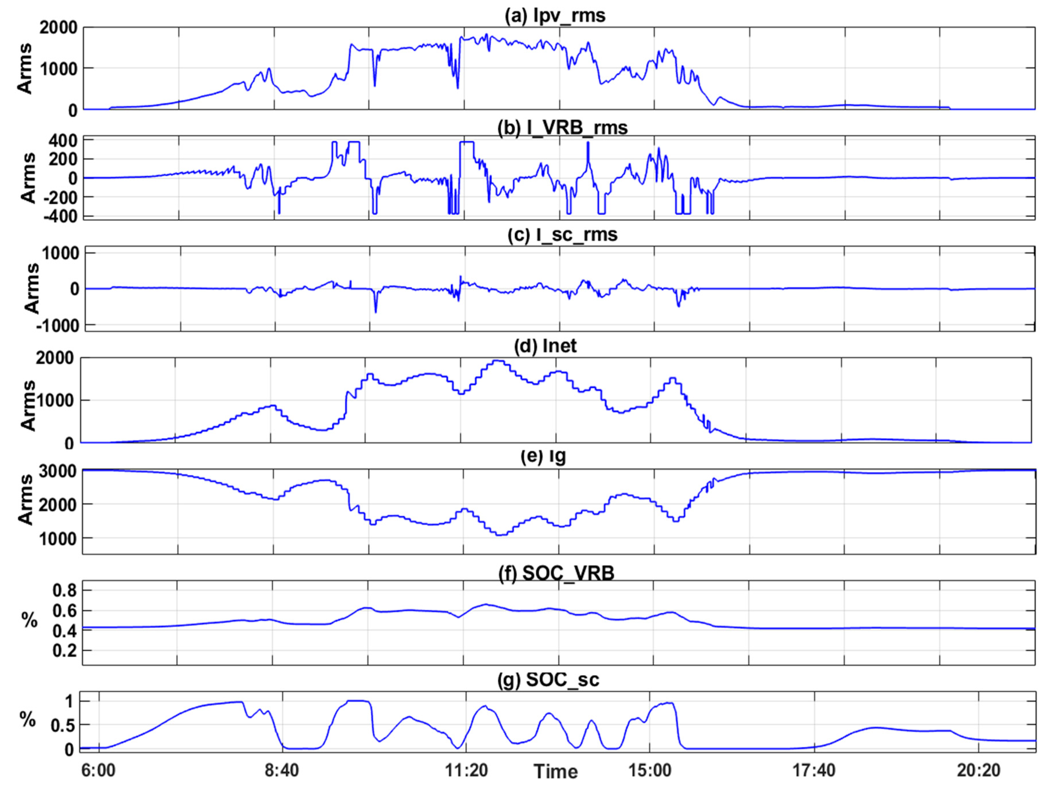
Figure 15 illustrates the system’s simulation using MATLAB Simulink. It is a PV system that generates three-phase AC current from the stored data, and the generator is comprised of a three-phase limited power source of 250kVA with a constant load of 220kVA. The controller is already derived in the flowchart shown in Figure 13 and Simulink in Figure 13 and Figure 14, and the SC and VRB have already been discussed. However, the bidirectional converter has been used as an averaged inverter to speed up the system simulation, and the transient has been neglected as a result. As shown in Error! Reference source not found., the collected data in (3/7) represent the current absorbed or supplied by the VRB, which is limited by (-380, 380A), as shown in the second row. The SC supplies or absorbs the current when the VRB current exceeds the limits, as shown in the third row. It is possible for the SC to absorb or supply current up to 1200A, but it does not exceed 1000A in this paper. PV, VRB, and SC supply the total current to the network in the fourth row. This appears to be the filtered current from the PV source. It almost does not change within 300 seconds. When VRB and SC reach their limits within very short periods, some overcurrent remains in the grid.
As a general principle, it minimizes the rapid and large changes that are supplied to the network and simplifies the groove control of the generator so that it can be applied with greater efficiency. Figure 17 shows the VRB and SC for the period (30/6-8/7), of which approximately 50% are within the 20%-80% range, which ensures VRB stability, efficiency, and lifetime. Since the VRB has a capacity smaller than a supercapacitor and its job is to recover fast changes in a short time, these changes almost disappear at low current since the VRB can handle small changes.
Figure 16.
Simulation results (a) The is the collected data in (3/7), (b) the current absorbs or supplied by the VRB, (c) the current absorbs or supplied by the SC, (d) The summation of currents ), (e) The generator current, (f) of VRB battery, (g) of capacitor SC.
Figure 16.
Simulation results (a) The is the collected data in (3/7), (b) the current absorbs or supplied by the VRB, (c) the current absorbs or supplied by the SC, (d) The summation of currents ), (e) The generator current, (f) of VRB battery, (g) of capacitor SC.
A simulation was conducted for three settlement periods (5,10, and 15 minutes), with battery storage sizes of 200kWh, 450kWh, and 750kWh, respectively. The SC size did not change over all periods, as shown in Figure 16, Figure 17 and Figure 18 for the three period’s data. Note that the currents of different sizes of batteries differ as well. The simulation outputs for the three (5,10, and 15-min) settlement periods ensure the SOC limitation minimizes penetration into the grid. Figure 15, Figure 16, Figure 17 and Figure 18 illustrate the simulated system without losses, transient effects, and load changes. It also assumes that the PV, ESS, and generator plants are connected, regardless of their location as discussed in [22,22]. Despite the importance of the previous variables in determining system efficiency, these variables have no significant effect on this research objective, which is the size of the ESS. It is assumed that transient problems of inverters do not affect ESS size due to their small losses in batteries and SC [24].
Furthermore, instead of direct communication between system parts, predicting grid stability in voltage and frequency can provide an excellent approach to changing sources. Finally, the load change has a clear effect, but it is assumed the grid was stable before adding the renewable source for future studies.
6. Conclusion
The hybrid ESS system was simulated using a high-power density device VRB and a high-energy density device SC. The size of the storage system was determined through Python testing, representing 10% of the PV instantaneous power during a five-minute settlement period. However, other research suggests that the ESS should be approximately 20%. In this scenario, with a battery capacity of 250 kWh and supercapacitors with a storage capacity of 26 kVA, the PV system could generate 2 MW of electricity. Additionally, settlement periods of 10 and 15 minutes were also tested. Many important factors were considered in the program development due to the limitations and lifespan of the VRB. In this simulation, a straightforward and effective control process was implemented. The SOC of both the VRB and SC remained within the optimal range by applying a simple factor derived from 0.5 added to the SOC. The system effectively utilized the output from PV renewable resources based on the ESS size determined by the Python code, adhering to the law of conservation of energy.
Furthermore, simulations were conducted for settlement periods of 10 and 15 minutes using actual data collected from a PV system in Malaysia. This method can be applied to any dataset by following the same steps; however, for non-tropical seasons, different seasonal factors must be considered.
References
- N. Ibrahim, S. Alwi, Z. Abd Manan, A. Mustaffa, K. Kidam, “Climate change impact on solar system in Malaysia: Techno-economic analysis” Renewable and Sustainable Energy Reviews, Volume 189, Part A, January 2024, 113901.
- L. Apa, L. D’Alvia, Z. Del Prete, E. Rizzuto, “Battery Energy Storage: An Automated System for the Simulation of Real Cycles in Domestic Renewable Applications”, 2023 IEEE 13th International Workshop on Applied Measurements for Power Systems (AMPS), 27-29 September 2023.
- M. Lundahl, H. Lappalainen, M. Rinne, M. Lundström, “Life cycle assessment of electrochemical and mechanical energy storage systems”, Energy Reports, Volume 10, November 2023, Pages 2036-2046. [CrossRef]
- Y. Yoo, G. Jang, S. Jung, “A Study on Sizing of Substation for PV With Optimized Operation of BESS”, IEEE ACCESS, Special Section on Evolving Technologies in ESS for Energy Systems Applications, Volume 8, 2020, pp 214577-214585.
- S. Bahramirad, W. Reder, A. Khodaei, “Reliability-Constrained Optimal Sizing of Energy Storage System in a Microgrid”, IEEE TRANSACTIONS ON SMART GRID, VOL. 3, NO. 4, Dec. 2012, pp 2056-2062. [CrossRef]
- F. Zhanga, A. Fub, L. Dinga, Q. Wua, B. Zhaod, P. Zie, “Optimal sizing of ESS for reducing AGC payment in a power system with high PV penetration”, International Journal of Electrical Power & Energy Systems, Vol. 110, 2019, pp 809-818.
- Bayram, M. Abdallah, A. Tajer, K. Qaraqe, “Energy storage sizing for peak hour utility applications,” 2015 IEEE International Conference on Communications (ICC), London, UK, 2015, pp. 770-775.
- Biyya, G. Aniba and M. Maaroufi, “Impact of load and renewable energy uncertainties on single and multiple energy storage systems sizing,” 2017 IEEE Power & Energy Society Innovative Smart Grid Technologies Conference (ISGT), Washington, DC, USA, 2017, pp. 1-5.
- Bechlenberg, E. Luning, M. Saltık, N. Szirbik, B. Jayawardhana, A. Vakis, “Renewable energy system sizing with power generation and storage functions accounting for its optimized activity on multiple electricity markets”, Applied Energy, Vol. 360, 2024. [CrossRef]
- M. Gomez-Gonzalez, J.C. Hernandez, D. Vera, F. Jurado, “Optimal sizing and power schedule in PV household-prosumers for improving PV self-consumption and providing frequency containment reserve”, Energy, Vol 191, 2020. [CrossRef]
- Etxeberria, I. Vechiu, S. Baudoin, H. Camblong, S. Kreckelbergh, “Control of a Vanadium Redox Battery and supercapacitor using a Three-Level Neutral Point Clamped converter”, Journal of Power Sources, Vol 248, 2014, pp 1170-1176. [CrossRef]
- J. Li, D. Hu, G. Mu, S. Wang, Z. Zhang, X. Zhang, X. Lv, D. Li, J. Wang, “Optimal control strategy for large-scale VRB energy storage auxiliary power system in peak shaving”, International Journal of Electrical Power & Energy Systems, Vol 120, 2020. [CrossRef]
- M. Ishaq, M. Yasir, P. Yusoff, A. Tariq, M. Sarikaya, M. Khan, “MXenes-enhanced vanadium redox flow batteries: A promising energy solution”, Journal of Energy Storage, Vol 96, 2024, 112711. [CrossRef]
- X. Li, Y. Song, Y. Qiu, D. Mu, Y. Ning, “Modeling and Simulation of MWh Vanadium Redox Batteries System”, 2023 IEEE 11th Joint International Information Technology and Artificial Intelligence Conference (ITAIC), 8-10 Dec. 2023, pp 1823-1830.
- Z. Zhenzhen, L. Qingquan, Z. Ruixiao, G. Pengfei, S. Weicheng, Z. Jinping, “Modeling and Simulation of External Characteristics of Vanadium Redox Flow Battery Energy Storage System”, The 6th IEEE Conference on Energy Internet and Energy System Integration (EI2), 11-13 November 2022, pp 2231-2235.
- Y. Challapuram, G. Quintero, S. Bayne, A. Subburaj; M. Harral, “Electrical Equivalent Model of Vanadium Redox Flow Battery”, 2019 IEEE Green Technologies Conference.
- D. Dong; P. Wang; W. Qin; X. Han, “Investigation of a Microgrid with Vanadium Redox Flow Battery Storages as a Black Start Source for Power System Restoration”, 2014 9th IEEE Conference on Industrial Electronics and Applications. [CrossRef]
- M. Sanjareh, M. Nazari, S. Hosseinian, “Optimal Supercapacitor Sizing for Enhancing Battery Life in Hybrid Energy Storage for Microgrid Energy Management”, IEEE, 2022 12th Smart Grid Conference (SGC), 13-15 December 2022.
- The International Renewable Energy Agency (IRENA), “Increasing Time-granularity in Electrisity Markets Innovation Landscape Brief” 2019, p13.
- IRENA (2023), Malaysia energy transition outlook, International Renewable Energy Agency, Abu Dhabi.
- M. Ceraolo, G. Lutzemberger, D. Poli, “State-Of-Charge Evaluation Of Supercapacitors”, Journal of Energy Storage, Volume 11, June 2017, Pages 211-218. [CrossRef]
- M. Järvelä, S. Valkealahti, “Comparison of AC and DC Bus Interconnections of Energy Storage Systems in PV Power Plants with Oversized PV Generator”, 16-21 June 2019, IEEE Photovoltaic Specialists Conference, (PVSC 46), Chicago, USA.
- Al-Bukhaytan, M. Abido, “A Planning Model for Optimal Capacity and Location of Energy Storage for Grid Inertial Support in Presence of Renewable Energy”, 2023 IEEE International Conference on Energy Technologies for Future Grids Wollongong, Australia, December 3-6, 2023.
- Z. Lu, J. Zhao, K. Tseng, K. Ng, Y. Rao, “Applying VRB-ESS in the DC micro-grid for green building electricity supply: Constructive suggestions to improve the overall energy efficiency”, 2013 IEEE 10th International Conference on Power Electronics and Drive Systems (PEDS), 22-25 April 2013, pp 130-135.
Figure 1.
The system block diagram.
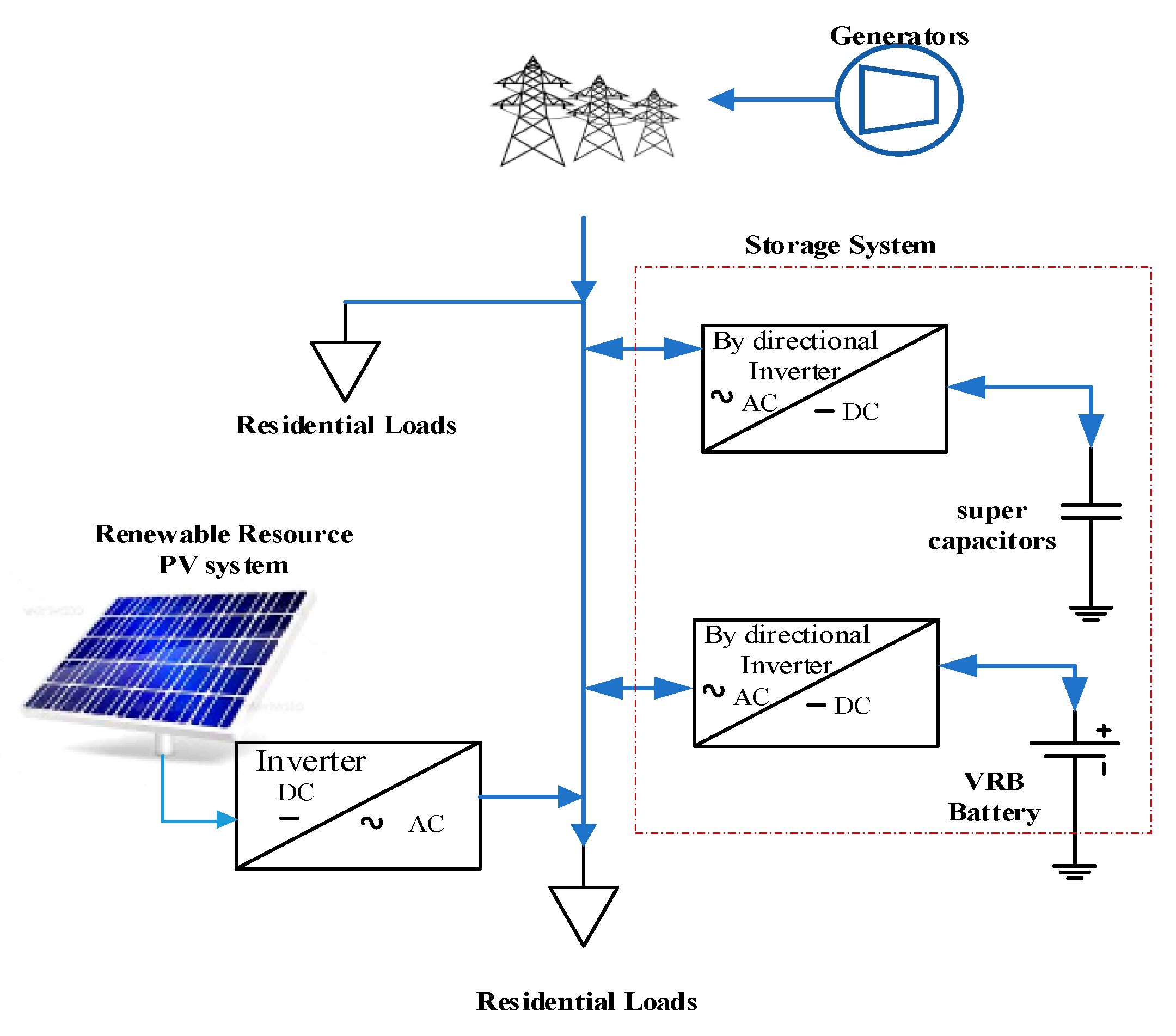
Figure 3.
(a) Power generated from the PV system in Malaysia between 30/June-8/July/21, (b) Expand of generated power at 3/Jul, (c) the system with averaging power with 8 hours.
Figure 3.
(a) Power generated from the PV system in Malaysia between 30/June-8/July/21, (b) Expand of generated power at 3/Jul, (c) the system with averaging power with 8 hours.
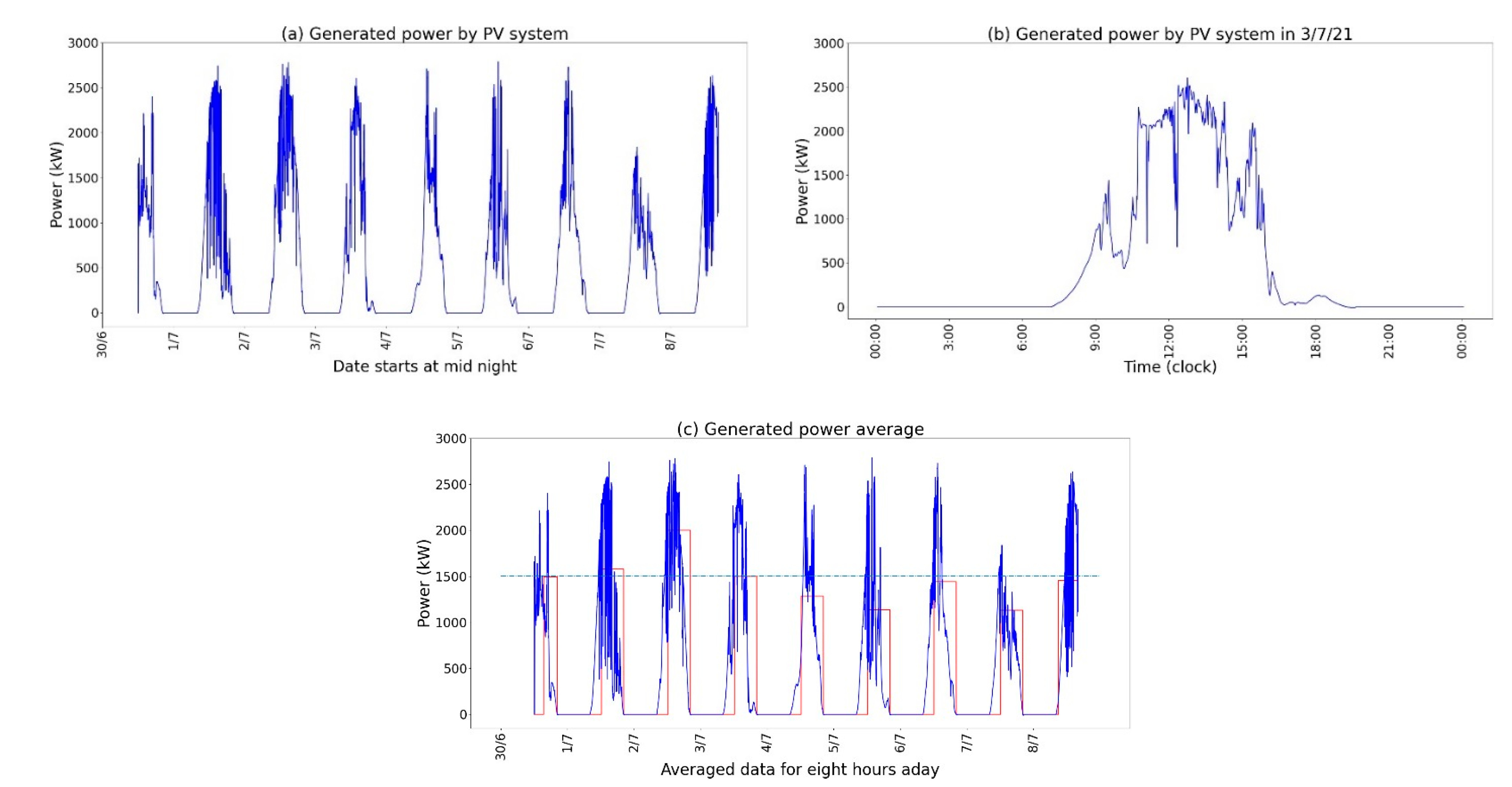
Figure 4.
Vanadium redox battery structure [13].
Figure 4.
Vanadium redox battery structure [13].
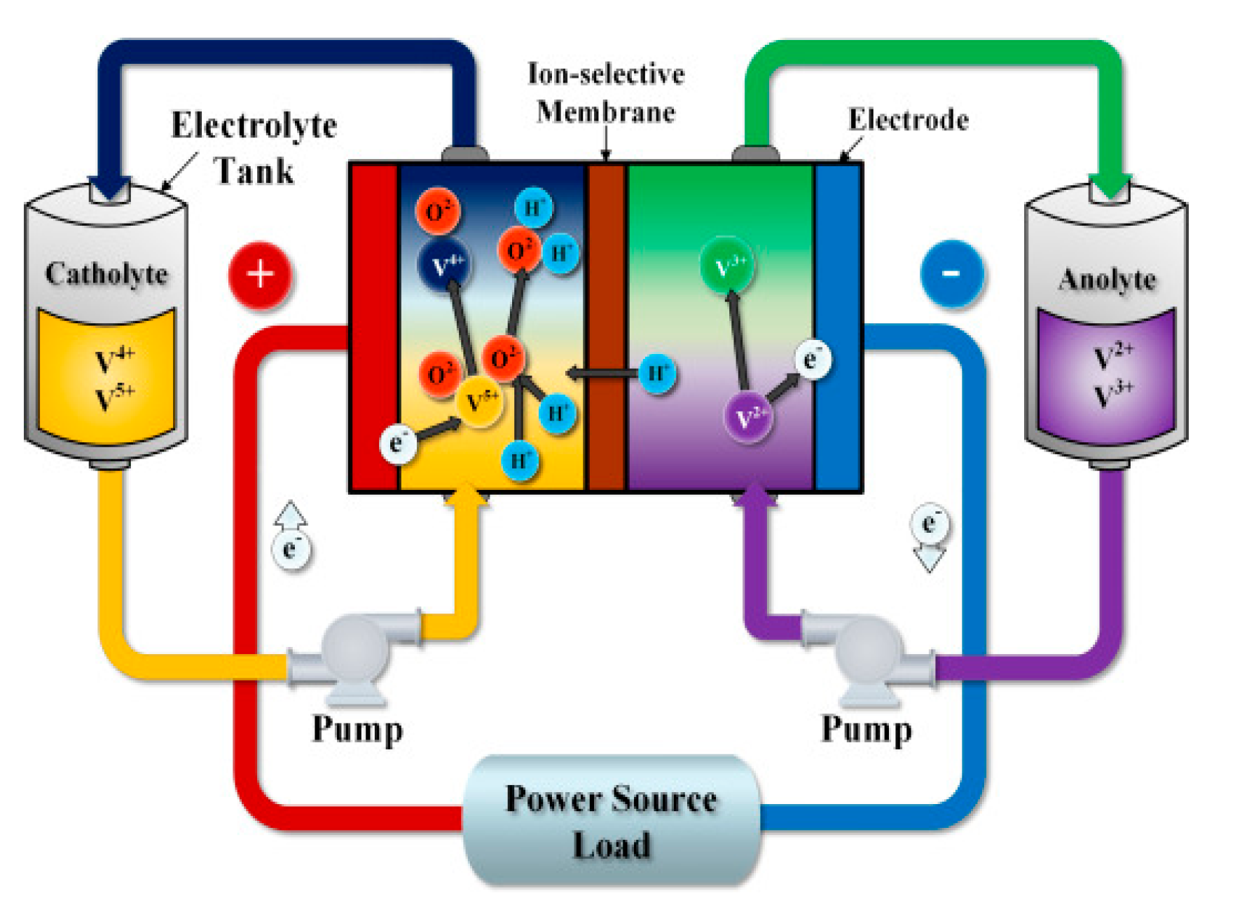
Figure 5.
Vanadium redox battery equivalent circuit.
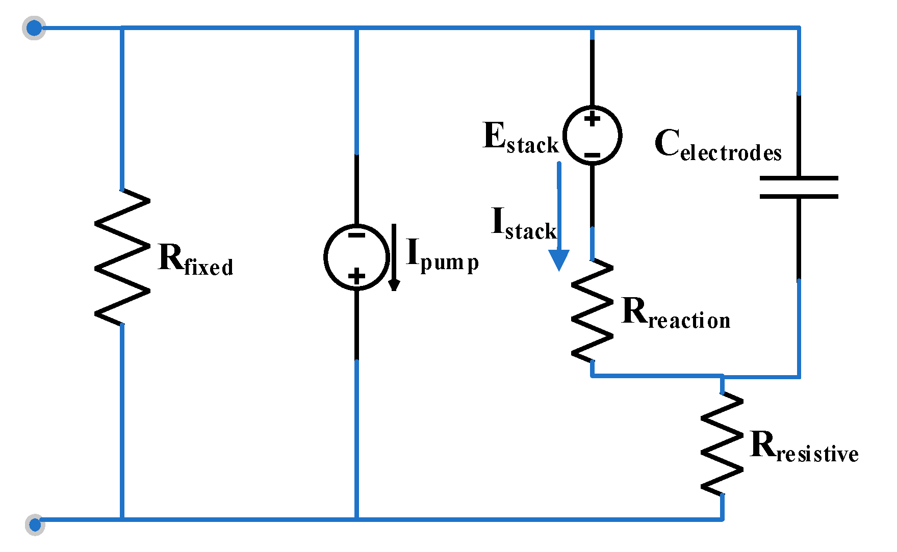
Figure 6.
Estack Estimator for the VRB.
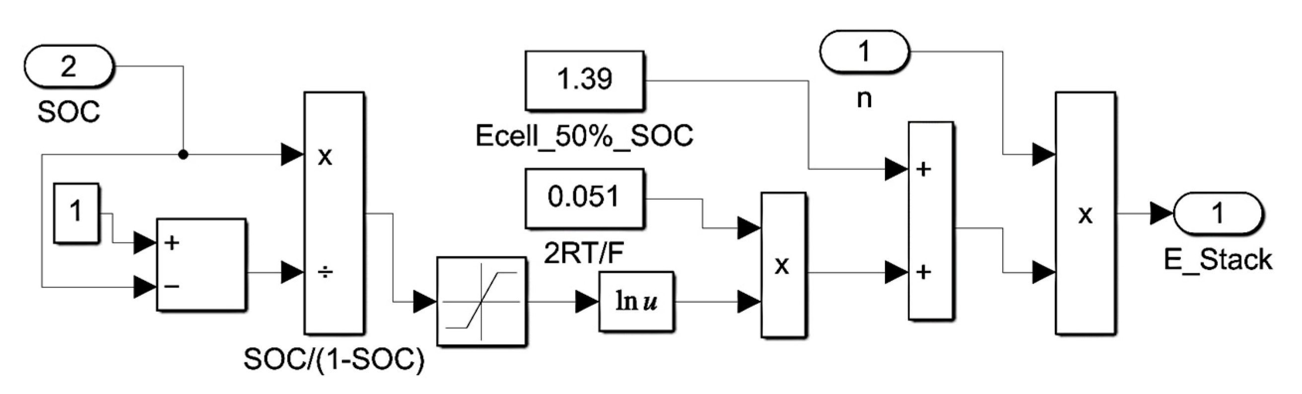
Figure 7.
SOC Estimator for VRB.
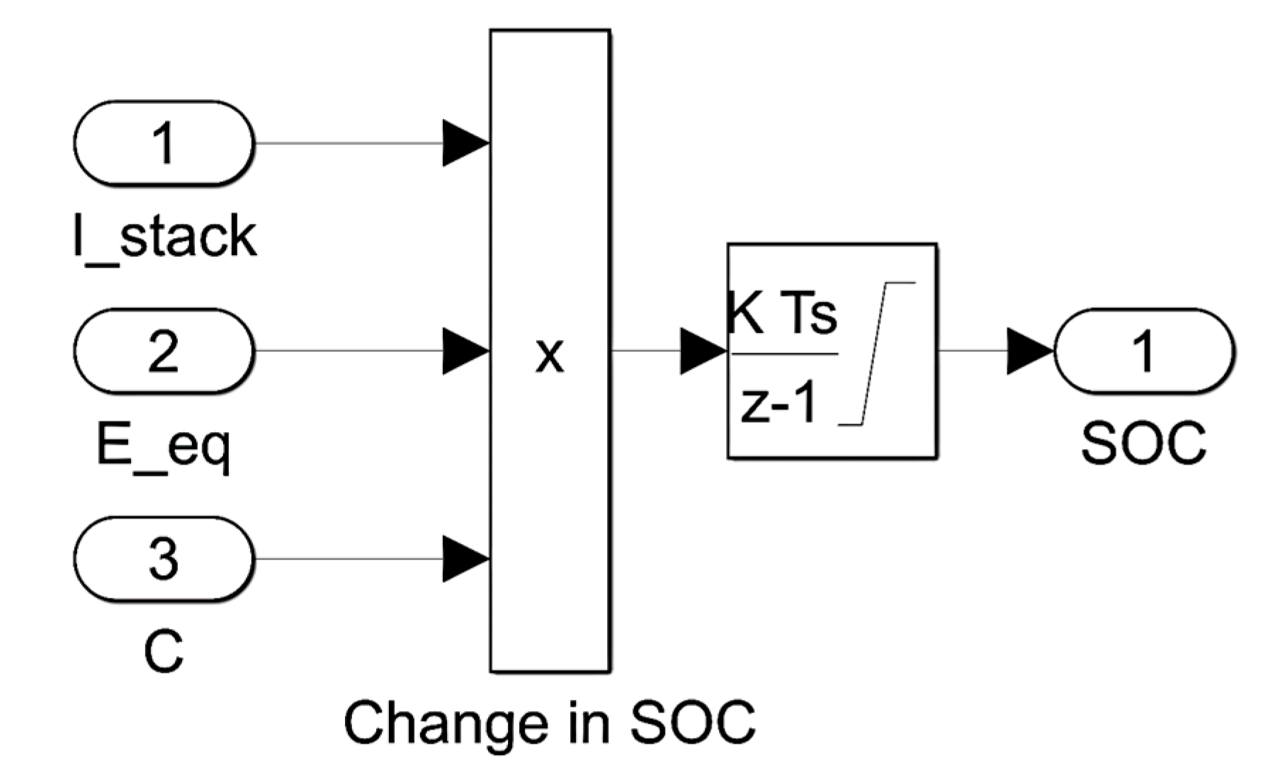
Figure 8.
Flow Q estimator for VRB.
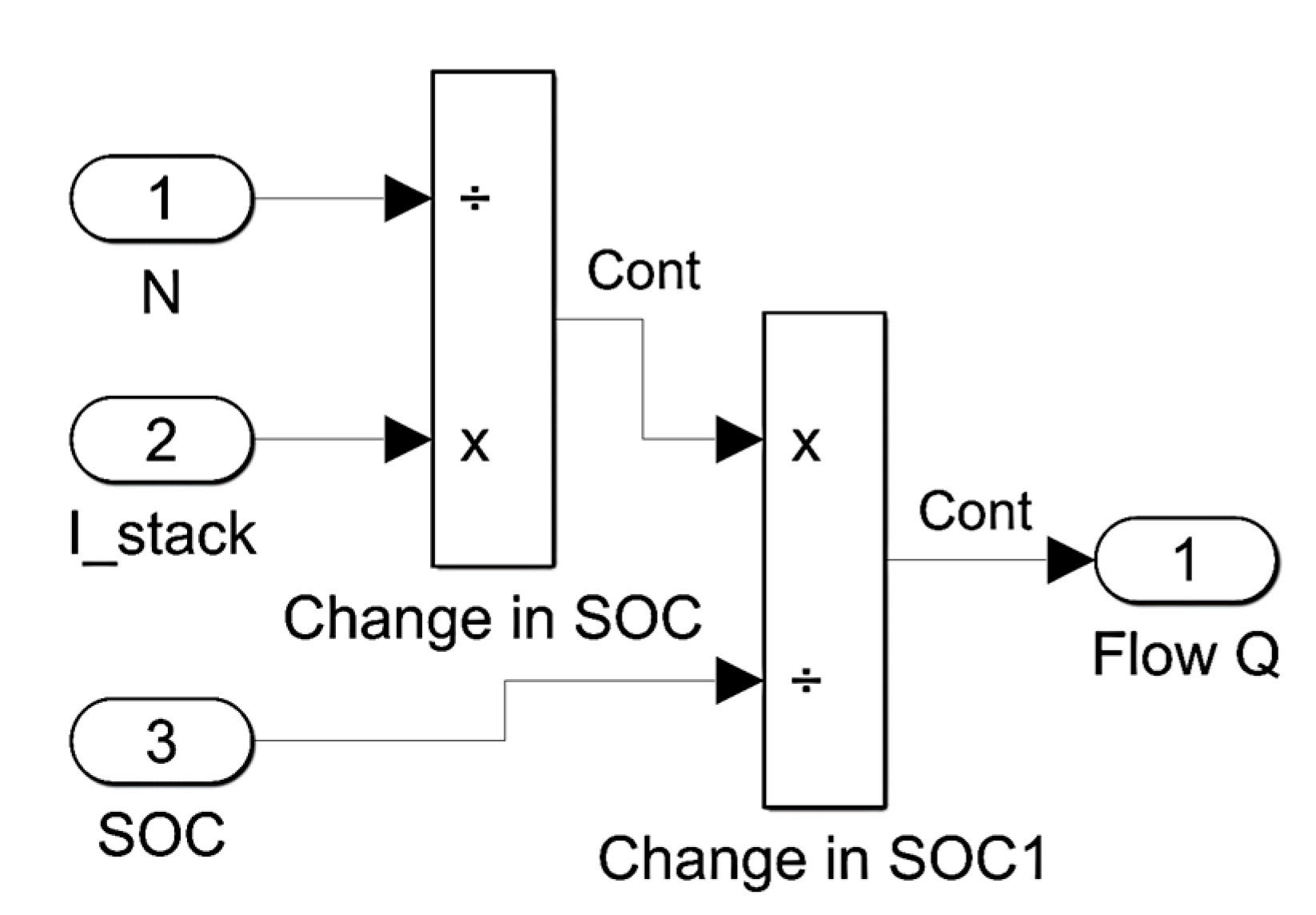
Figure 9.
VRB model simulated using SIMULINK.
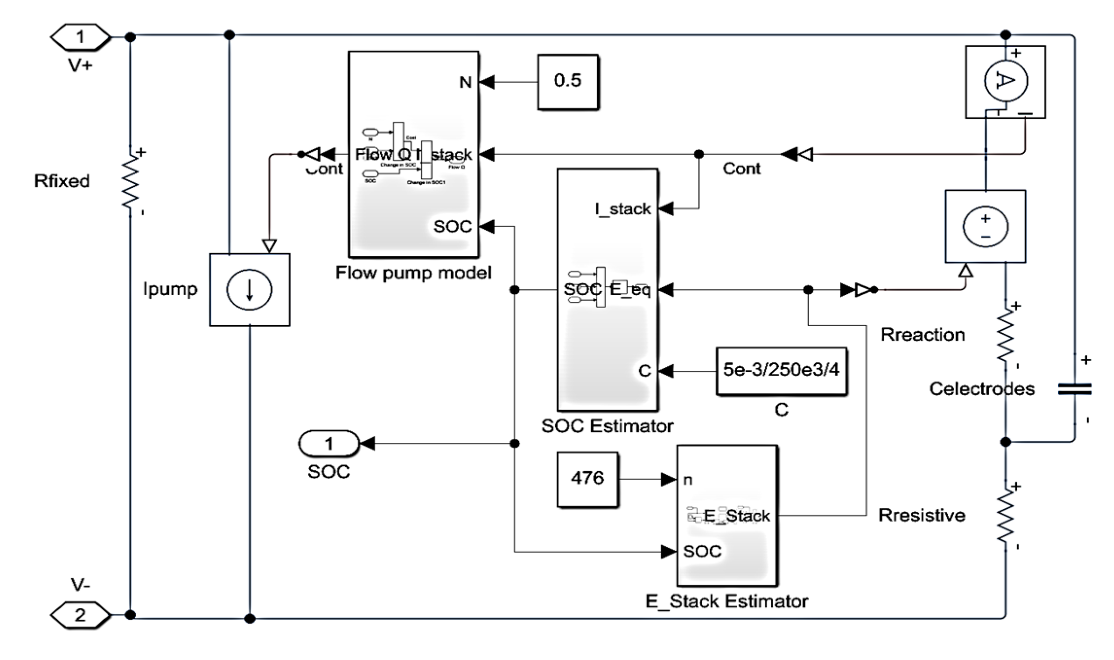
Figure 10.
VRB model output shows the SOC change with maximum power applied.
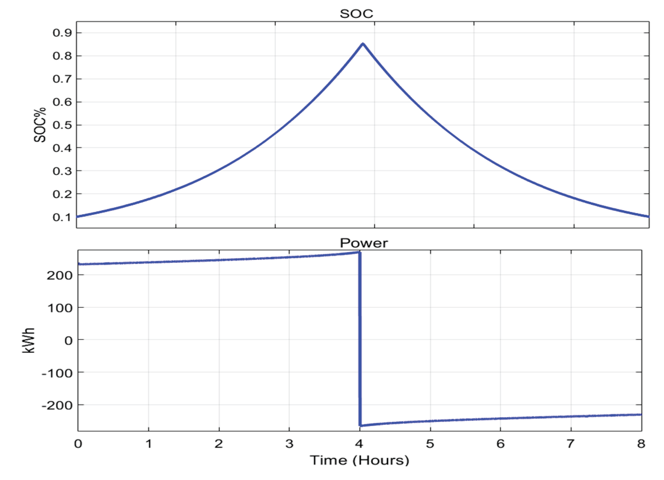
Figure 11.
The relation between the storage system size and the energy loss percentage in an ideal case.
Figure 11.
The relation between the storage system size and the energy loss percentage in an ideal case.
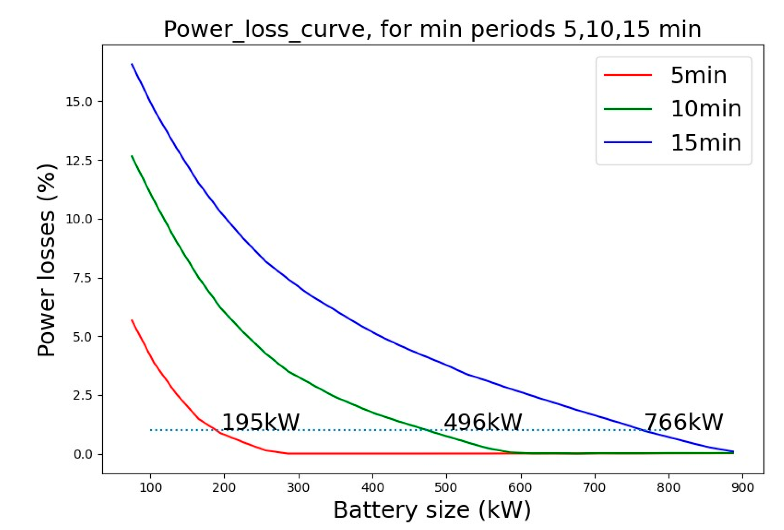
Figure 12.
Battery charge and discharge control process flow chart.
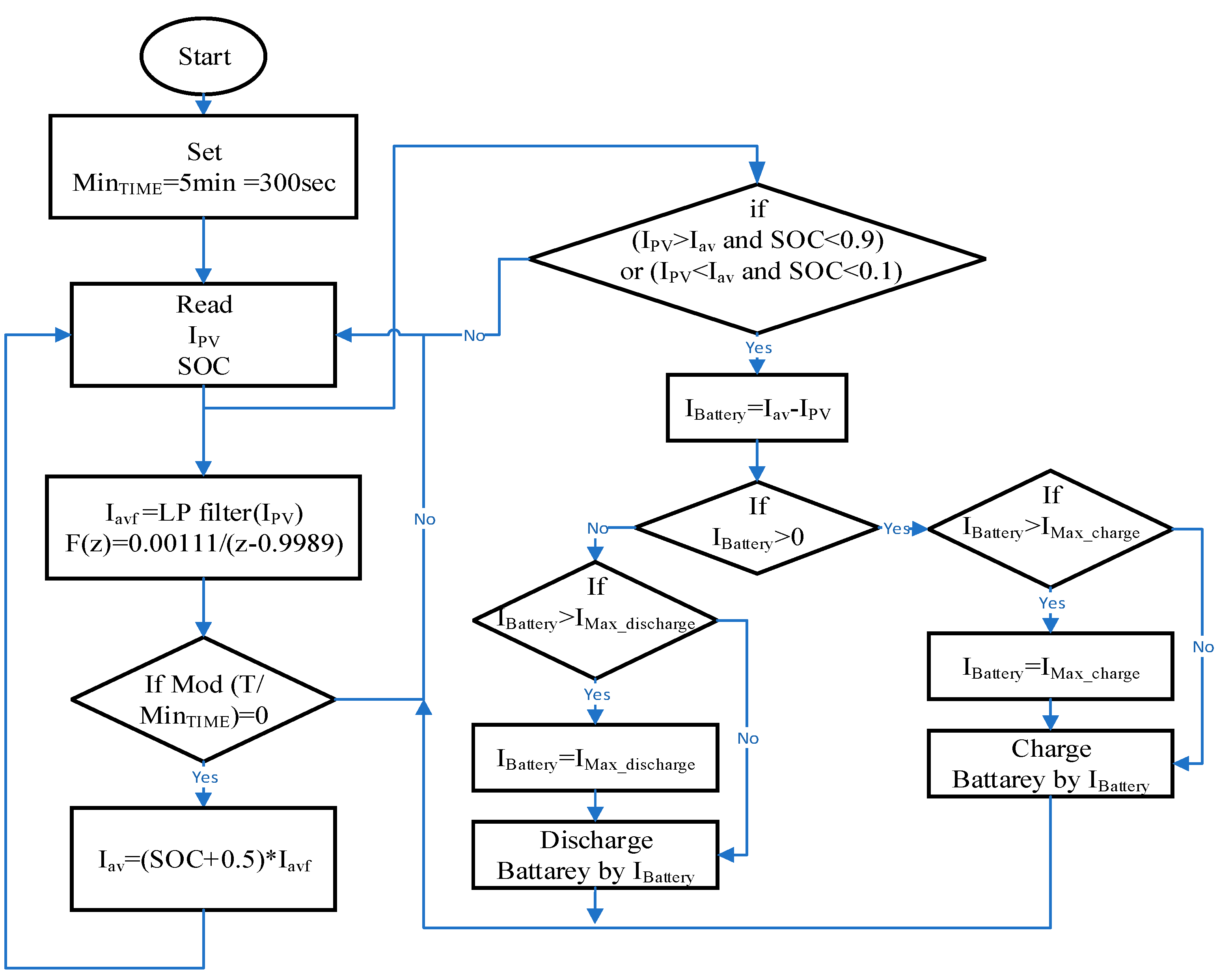
Figure 13.
VRB and SC charge and discharge control flowchart.
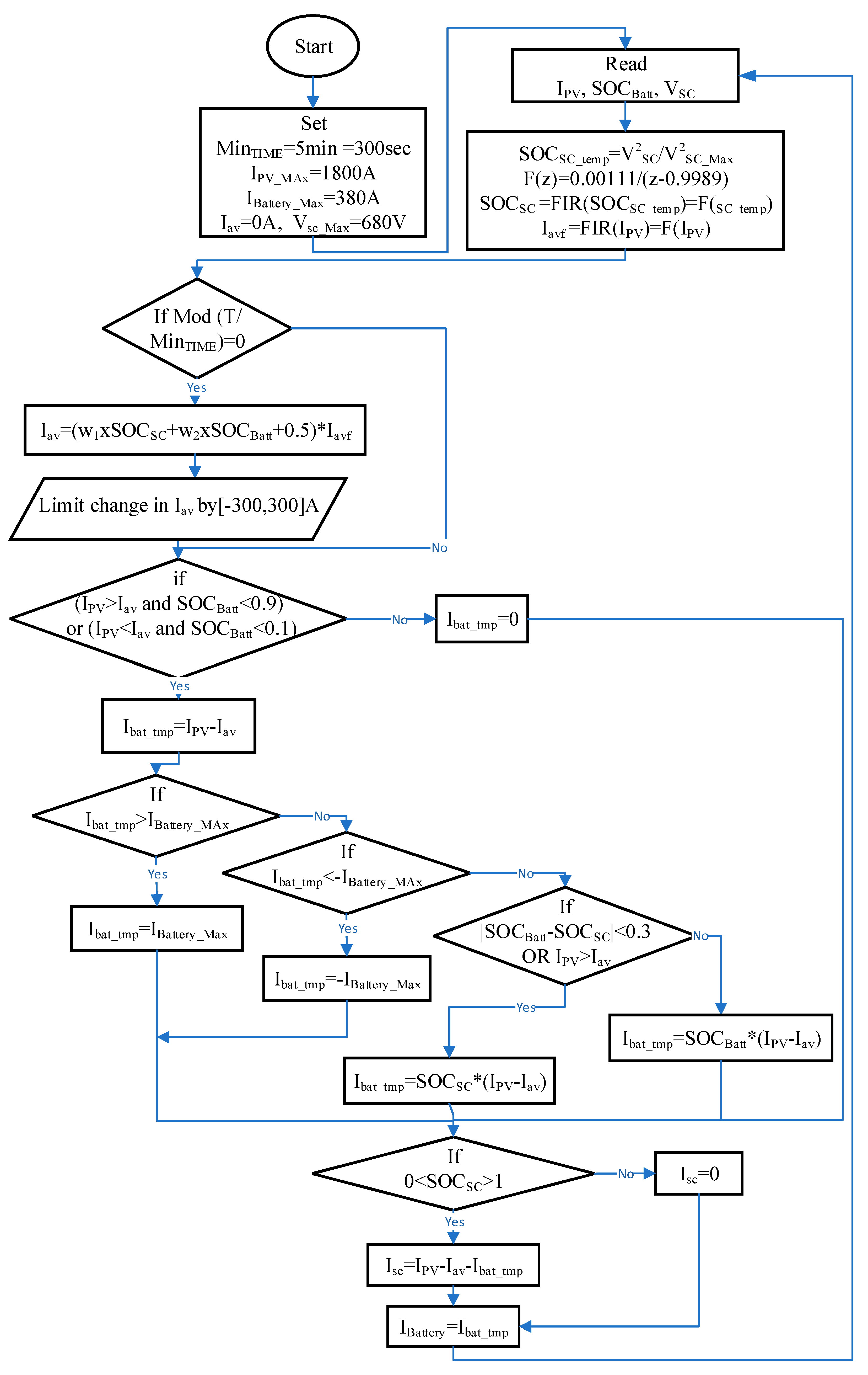
Figure 14.
Iav generation by Simulink.
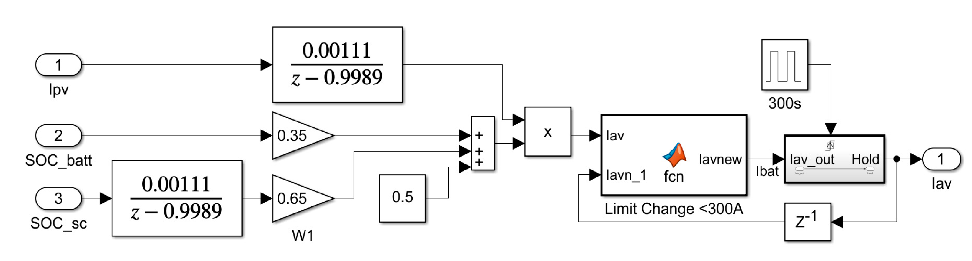
Figure 15.
IBatt and Isc generation by Simulink.
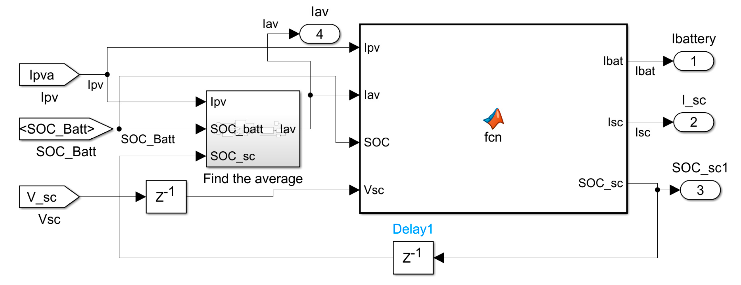
Figure 17.
Simulation results for a 5-min settlement period for the collected data in (30/6-8/7): (a) The is, (b) the current absorbs or supplied by the VRB, (c) the current absorbs or supplied by the SC, (d) The summation of currents), (e) The generator current, (f) of VRB battery, (g) of capacitor SC.
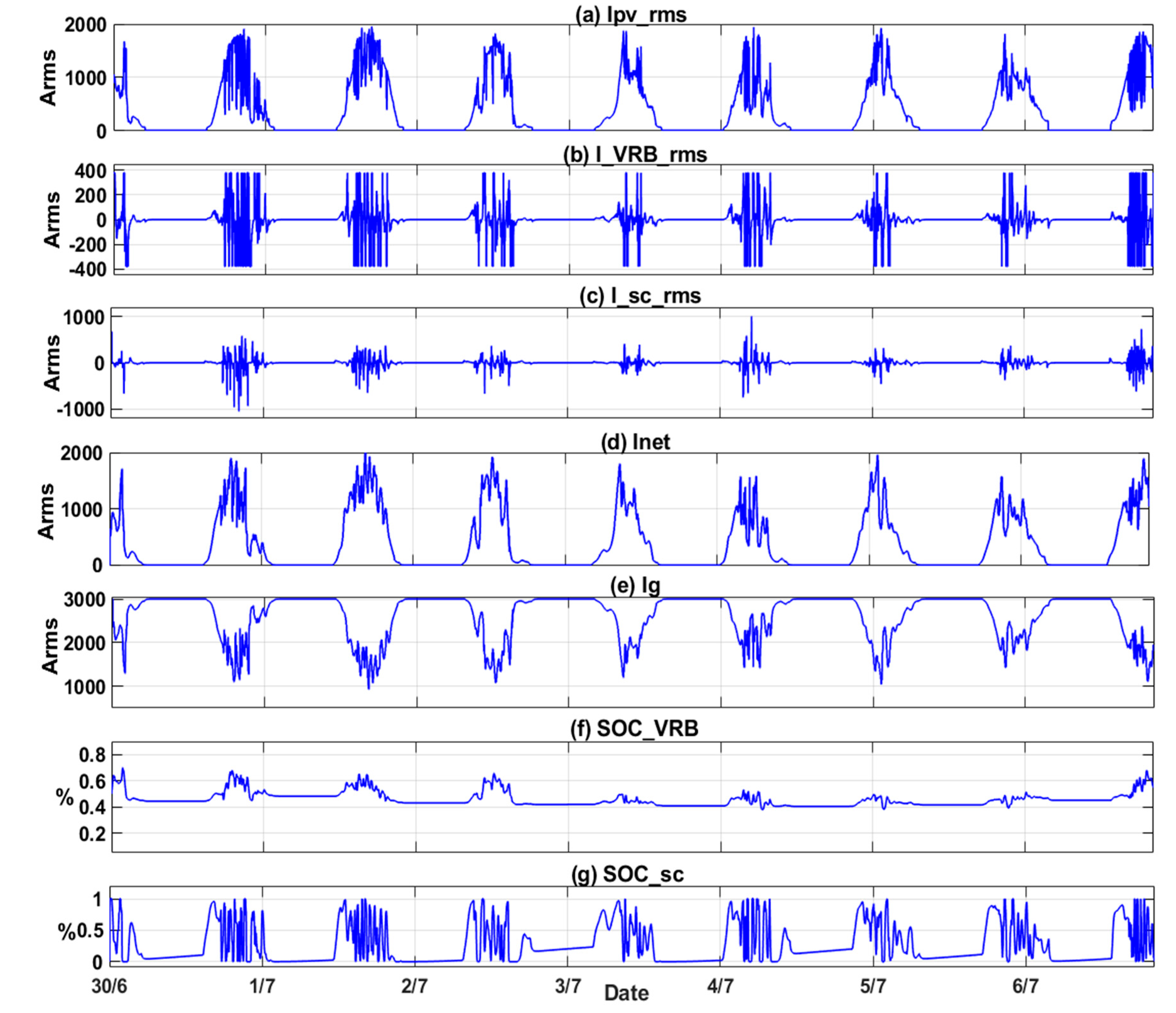
Figure 18.
Simulation results for 10-min settlement period for the collected data in (30/6-8/7): (a) the current absorbs or supplied by the VRB, (b) the current absorbs or supplied by the SC, (c) The generator current, (d) of VRB battery, (e) of capacitor SC.
Figure 18.
Simulation results for 10-min settlement period for the collected data in (30/6-8/7): (a) the current absorbs or supplied by the VRB, (b) the current absorbs or supplied by the SC, (c) The generator current, (d) of VRB battery, (e) of capacitor SC.
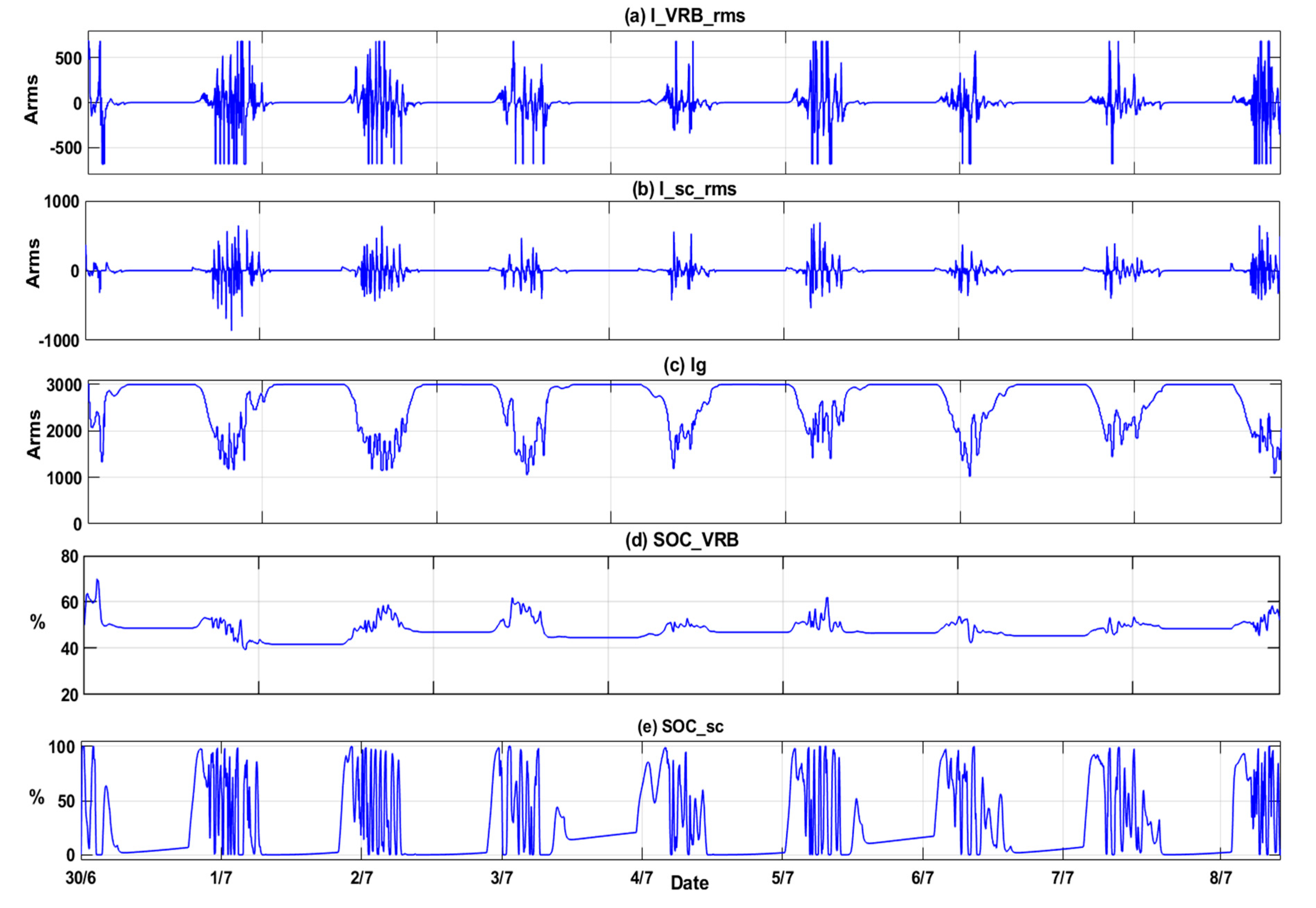
Figure 19.
Simulation results for 15-min settlement period for the collected data in (30/6-8/7): (a) the current absorbs or supplied by the VRB, (b) the current absorbs or supplied by the SC, (c) The generator current, (d) of VRB battery, (e) of capacitor SC.
Figure 19.
Simulation results for 15-min settlement period for the collected data in (30/6-8/7): (a) the current absorbs or supplied by the VRB, (b) the current absorbs or supplied by the SC, (c) The generator current, (d) of VRB battery, (e) of capacitor SC.
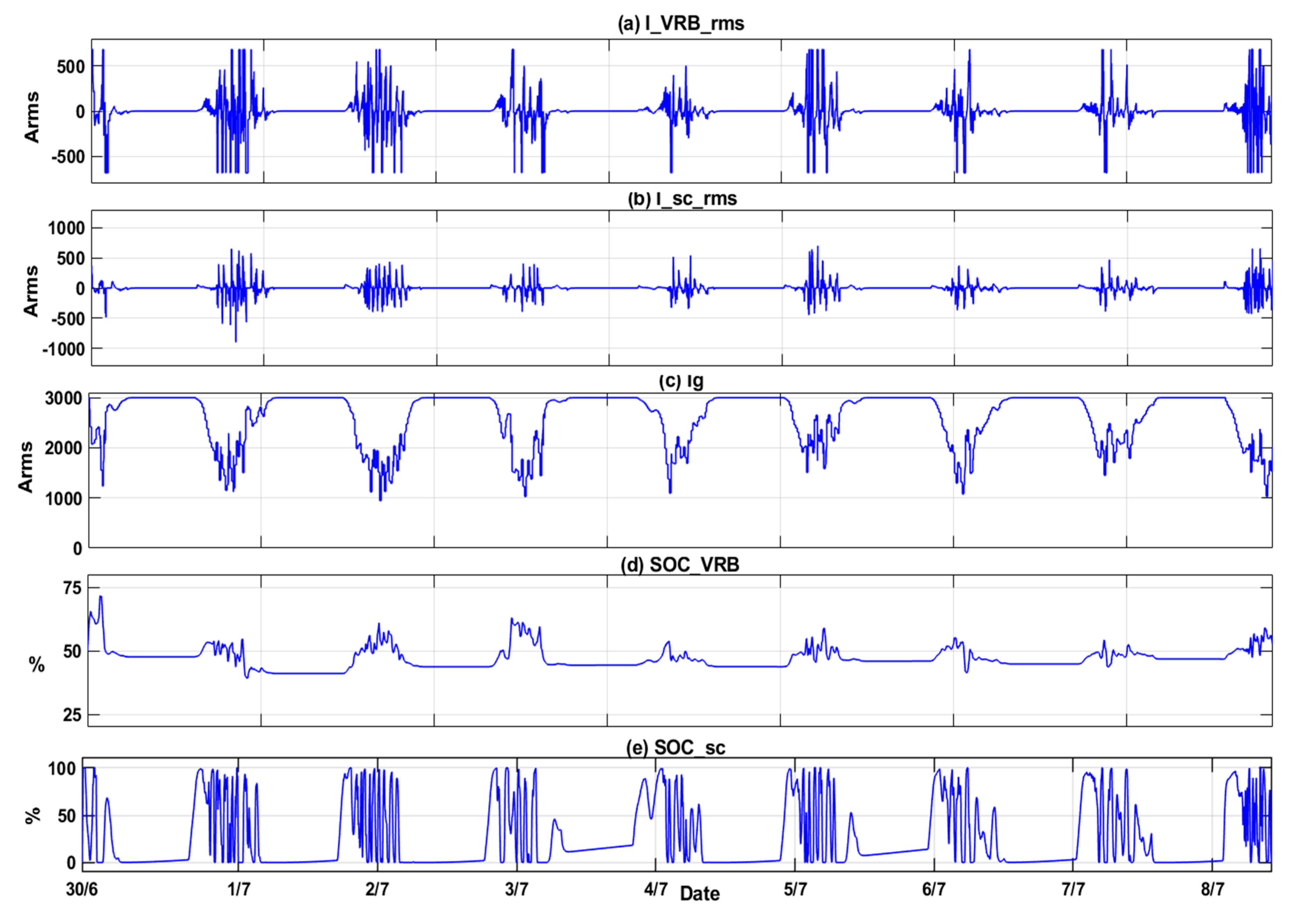

Table 1.
Product Specifications of used VRB.
| Power rating output | 250kW |
| Overload capability | Discharge: 30% 1 hour, SOC is >60% Charge: 25% 45 minutes, SOC is <25% |
| Storage Duration | 2 to 8 hours |
| DC bus voltage | 300 to 800V |
| Self-discharge %/day | 0.05% |
Table 2.
Product Specifications of SC.
| Rated Capacitance | 165 F |
| Maximum ESR DC, initial | 6.3 mΩ |
| Rated Voltage | 48 V |
| Absolute Maximum Current | 1,900 A |
| Maximum Series Voltage | 750 V |
| Stored Energy | 53 Wh |
Disclaimer/Publisher’s Note: The statements, opinions and data contained in all publications are solely those of the individual author(s) and contributor(s) and not of MDPI and/or the editor(s). MDPI and/or the editor(s) disclaim responsibility for any injury to people or property resulting from any ideas, methods, instructions or products referred to in the content. |
© 2025 by the authors. Licensee MDPI, Basel, Switzerland. This article is an open access article distributed under the terms and conditions of the Creative Commons Attribution (CC BY) license (http://creativecommons.org/licenses/by/4.0/).
Copyright: This open access article is published under a Creative Commons CC BY 4.0 license, which permit the free download, distribution, and reuse, provided that the author and preprint are cited in any reuse.


