
Submitted:
13 May 2025
Posted:
14 May 2025
You are already at the latest version
Abstract
The statistical mechanics of structured particles with arbitrary size and shape adsorbed on discrete lattices presents a longstanding theoretical challenge, mainly due to complex spatial correlations and entropic effects that emerge at finite densities. Even for simplified systems like hard-core linear k-mers, exact solutions remain limited to low-dimensional or highly constrained cases. In this review, we present a comprehensive analysis of theoretical approaches developed to describe adsorption phenomena involving structured particles (also known as multisite-occupancy adsorption) on regular lattices. We examine classical models including the Flory–Huggins and Guggenheim–DiMarzio theories, modern extensions such as an extension to two dimensions of the exact thermodynamic functions obtained in one dimension, the Fractional Statistical Theory of Adsorption based on Haldane’s fractional statistics, and the so-called Occupation Balance based on the expansion of the reciprocal of the fugacity, and hybrid approaches like the Semiempirical model obtained by combining exact one-dimensional calculations and Guggenheim–DiMarzio approach. For interacting systems, statistical thermodynamics is explored within generalized Bragg–Williams and quasi-chemical frameworks. Particular focus is given to the recently proposed Multiple Exclusion statistics, which capture the correlated exclusion effects inherent to non-monomeric particles. Applications to monolayer and multilayer adsorption are analyzed, with relevance to hydrocarbon separation technologies. Finally, computational strategies, including advanced Monte Carlo techniques, are reviewed in the context of high-density regimes. This work provides a unified framework for understanding entropic and cooperative effects in lattice-adsorbed polyatomic systems and highlights promising directions for future theoretical and computational research.
Keywords:
multisite-occupancy adsorption
; lattice-gas models
; statistical thermodynamics
1. Introduction
Understanding the statistical mechanics of structured particles with arbitrary size and shape in external fields remains a major theoretical challenge, largely due to the complex entropic contributions arising from particle configurations at finite densities. Even for simplified models, such as linear particles with hard-core interactions on regular lattices, the problem is analytically intractable. This difficulty stems from spatial correlations among allowed particle configurations, which complicate the calculation of thermodynamic potentials. These correlations underlie various emergent collective behaviors, including nematic ordering in systems of linear k-mers [1], and entropy-driven competition in multicomponent mixtures. Exact solutions have been found only in a few special cases, such as dimers on square lattices [2] and hexagons on regular lattices [3].
In continuum systems, this problem has been extensively studied. In three-dimensional colloidal suspensions, Onsager famously demonstrated that elongated molecules undergo a phase transition from an isotropic to a nematic phase [1]. In two dimensions, although continuous rotational symmetry cannot be spontaneously broken, a Kosterlitz–Thouless transition occurs, characterized by a power-law decay in orientational correlations [4,5].
In contrast, the case of hard-core particles on lattices is less well understood. Early work by Flory [6] and Huggins [7] initiated the study of rigid rods, or k-mers, modeled as linear arrangements of k identical units occupying contiguous lattice sites. These rods interact solely through hard-core exclusion, meaning that no site may be occupied by more than one unit.
The Flory–Huggins () theory, developed independently by Flory [6] and Huggins [7], generalizes the theory of binary liquid mixtures or dilute polymer solutions on lattices. In the lattice–gas framework, the adsorption of k-mers on homogeneous surfaces is formally analogous to polymer–solvent binary solutions.
Extensive efforts have been made to assess theory against experimental results, the theory being completely satisfactory in a qualitative, or semi-quantitative way. There is no doubt that this simple theory contains the essential features which distinguish high polymer solutions from ordinary solutions of small molecules. Modified forms of the approximation have been also proposed. A comprehensive discussion on this subject is included in the book by Des Cloizeaux and Jannink [8].
The statistics, given for the packing of molecules of arbitrary shape but isotropic distribution, provides a natural foundation onto which the effect of the orientation of the ad-molecules can be added. Following this line of thought, DiMarzio [9] developed an approximate method of counting the number of ways, , to pack together linear polymer molecules of arbitrary shape and of arbitrary orientations. Accordingly, was evaluated as a function of the number of molecules in each permitted direction. These permitted directions can be continuous so that is derived as a function of the continuous function which gives the density of rods lying in the solid angle , or the permitted directions can be discrete so that is the the number of ways to pack molecules onto a lattice. Based on the detailed knowledge of the orientations of the molecules, the various types (nematic, smetic, and cholestic) of liquid crystals were argued for and the reasons for their existence were ascertained. In the case of allowing only those orientations for which the molecules fit exactly onto the lattice is that for the case of an isotropic distribution the value of reduces to the earlier result by Guggenheim [10], now known as the Guggenheim–DiMarzio () approximation.
In the 2000s, two novel approaches were proposed for describing multisite adsorption. The first, developed by Ramirez-Pastor et al. [11], introduced the Extension Ansatz () model for linear adsorbates on homogeneous surfaces, based on exact one-dimensional thermodynamic expressions and their generalization to higher dimensions. The second, the Fractional Statistical Theory of Adsorption () [12,13], incorporates the internal configuration of the adsorbed molecule as a model parameter. generalizes Haldane’s fractional exclusion statistics [14,15], originally developed for quantum systems, to describe classical polyatomic adsorption at gas–solid interfaces.
Comparisons with simulation data [11] have shown that the approximation agrees well at low surface coverage, while the model performs better at high coverage. These insights led to the development of the Semiempirical () Model for Polyatomic Adsorption [11,16], a hybrid model combining exact 1D results with approximations, weighted appropriately.
More recently, the Multiple Exclusion () statistics framework was introduced to describe classical systems in which particles access spatially correlated states [17,18]. statistics accounts for situations in which multiple particles simultaneously exclude access to a common state, an intrinsic feature of non-monomeric particles on a lattice. The uncorrelated limit of statistics recovers both the Haldane-Wu and formalisms. This approach was further extended in Ref. [19] to mixtures of particles with arbitrary shapes and sizes, allowing for analytical expressions of thermodynamic quantities in terms of coverage and species densities.
Despite the number of studies dealing with the adsorption of polyatomics on discrete lattices, there are many aspects which are still outstanding. While the problem can be easily and precisely defined, exact solutions for adsorbed correlated particles, such as k-mers, have historically proved elusive, with results being limited to one-dimensional substrates [20] and a few shapes in dimensions greater than one. The classic example of such a model is the lattice-gas of dimers () [2,21,22,23,24,25,26,27,28]. A review on the entropy of fully packed dimers on planar lattices may be found in Ref. [29].
The inherent complexity of the k-mer problem is further increased when attempting to obtain approximate solutions for the thermodynamic functions of systems that, in addition to allowing multiple site occupancy, also involve lateral interactions among adsorbed molecules and/or surface heterogeneity. In this context, simple solvable models of adsorption on homogeneous surfaces serve as valuable foundations for developing alternative approaches to more complex cases involving interacting adsorbates [30,31] and heterogeneous surfaces [32,33,34,35,36,37].
In this work, we present a comprehensive overview of foundational and recent theoretical developments in the modeling of structured particle adsorption on regular lattices (commonly referred to as multisite occupancy adsorption). We focus on how particle geometry and size affect the configurational entropy of the adsorbed layer, an aspect that has rarely been systematically treated in thermodynamic models. Understanding entropic effects in polyatomic systems is particularly relevant for applications such as alkane and hydrocarbon adsorption, which are key to petrochemical separation technologies.
The paper is structured as follows: Section 2 examines the thermodynamics of one-dimensional lattice gases composed of interacting and non-interacting linear particles, covering both single-species and mixture adsorption, including monolayer and multilayer regimes. Section 3 presents theoretical approximations for non-interacting polyatomic species in two dimensions, including the and models, the extension of one-dimensional results, the framework based on fractional statistics, the Occupation Balance () approximation, and the model. Adsorption of single and multicomponent species is discussed in both monolayer and multilayer contexts. Section 4 explores two-dimensional lattice gases of interacting structured species via mean-field and quasi-chemical approaches. Intermolecular interactions give rise to possible phase transitions. Section 5 introduces the statistics framework for classical lattice gases of arbitrarily shaped particles, generalizing the formalism of multiple exclusion statistics presented in Ref. [18]. Section 6 extends statistics to multicomponent systems, analytically describing the exclusion spectra in terms of lattice coverage and species densities. This appears as a suitable framework to address complex lattice gases mixtures where spatial state correlations are significant to understand their phase behavior. Section 7 discusses applications of the main theoretical models developed in this review, comparing model predictions with Monte Carlo simulations and experimental data. Section 8 focuses on computational methods. The statistics of polyatomics is also a very demanding problem from a computational point of view. Whereas for monomer particles () the thermal equilibrium is quickly reached using standard adsorption–desorption MC algorithms, the relaxation time for large particles increases very quickly as the density increases. Consequently, MC simulations are very time consuming at high density and produce artefacts related to non-accurate equilibrium states. In order to cope with these difficulties, efficient MC simulations based on cluster moves were developed in the literature. The use of these techniques has made it possible to investigate the behavior of the system at high densities. In Section 8, the main computational algorithms of interest for the study of adsorption problems involving multiple-site occupancy are presented. Most of these algorithms have been used throughout the present work. Finally, Section 9 presents our conclusions and future perspectives.
2. Thermodynamic Functions of Lattice Gases of Polyatomics in One Dimension: Exact Solutions for Single Species and Mixtures
In the last decades, the advent of modern techniques for building single and multi-walled carbon nanotubes [38,39,40,41,42] has considerably encouraged the investigation of the gas-solid interaction (adsorption and transport of simple and polyatomic adsorbates) in such a low dimensional confining adsorption potentials.
The design of carbon tubules, as well as of synthetic zeolites and aluminophosphates such as [43] having narrow channels, literally provides a way to the experimental realization of one-dimensional (1D) adsorbents. The 1D character of adsorption in troughs of surface crystal planes of TiO2 has also been reported [44].
Many studies on conductivity, electronic structure, mechanical strengh, etc. of carbon nanotubes are being currently carried out. However the amount of theoretical and experimental work done on the interaction and thermodynamics of simple gases adsorbed in nanotubes is still very limited [45,46,47,48].
For theoretical modelling purposes, the adsorption potential within the narrowest nanotubes can be matched to a homogeneous 1D lattice M of adsorption sites (1D lattice-gas approach). This is, of course, an approximation to the state of real adsorbata in nanotubes which is justified because thermodynamics and transport coefficient can be analytically resolved in these conditions. This is of much qualitative value and may be thought feasible for monoatomic species strongly bonded to the nanopores’s wall, as well as for polyatomics where the distance between their building units do not seriously mismatch the separation between adsorption potential minima for single units.
In this section, we present the exact solution for the thermodynamics functions of non-interacting linear chains (k-mers) of arbitrary length adsorbed in a infinite 1D space (Section 2.1.1). The thermodynamic functions are further extended to binary mixtures (Section 2.1.2) and multilayer adsorption (Section 2.1.3). Section 2.2.1 and Section 2.2.2 are devoted to interacting single and multicomponent species, respectively.
2.1. One-Dimensional Model of Non-Interacting Structured Particles
2.1.1. Exact Solution for Rigid Particles on a 1D-Lattice: Single Species
Let us assume a one-dimensional lattice of M sites with lattice constant a () where periodic boundary conditions apply. Under this condition all lattice sites are equivalent hence border effects will not enter our derivation.
N linear k-mers are adsorbed on the lattice such a way that each k-mer unit (monomer) occupies one lattice site and double site occupancy is not allowed as to represent properties in the monolayer regime. The only interaction between different rods is hard-core exclusion: no site can be occupied by more than one k-mer’s unit. Since different k-mers do not have additional interactions between each other, all configurations of N k-mers on M sites are equally probable; henceforth, the canonical partition function equals the total number of configurations, , times a Boltzmman factor including the total interaction energy between k-mers and lattice sites,
Since the lattice is assumed homogeneous, , where is the interaction energy between every unit forming a k-mer and the substrate.
can be readily calculated as the total number of permutations of the N indistinguishable k-mers out of entities, being
Accordingly,
(a particular solution for dimers was presented in [49]).
In the canonical ensemble the Helmholtz free energy relates to through
where .
The remaining thermodynamic functions can be obtained from the general differential form [50]
where S, and designate the entropy, spreading pressure and chemical potential respectively, which, by definition, are
Thus, from Equations (3) and (4)
which can be accurately written in terms of the Stirling’s approximation
Henceforth, from Equations (6) and (8)
and
Then, by defining the lattice coverage , molar free energy and molar entropy , Equations (8)–(11) can be rewritten in terms of the intensive variables and T,
and
where .
The Equation (15) is the exact, so-called, isotherm equation for k-mers in one dimension which should be regarded as a generalization of the well-known equation
(where holds for Flory-Huggins’s approximation) developed by Flory [6] and Huggins [7] for polymer solutions when the solvent is monomeric with unitary molar volume. This is indeed isomorphic with the case analyzed in the present work, where the empty sites of the lattice formally correspond to the solvent’s monomers in Flory’s solution.
The explicit forms for the molar free energy and entropy from Flory-Huggins’s approximation are,
and
An extensive comparison between the exact isotherm Equation (15) and Flory-Huggins’s equation, along with MC simulations is shown in Figure 1. The simulations were developed using the scheme presented in Section 8.1.1 for one-dimensional lattices with sites, MCSs and MCSs. Since the lattice is assumed homogeneous, is arbitrarily chosen equal to zero without losing generality. Flory-Huggins’s approximation agrees fairly well with the exact result for very small k-mers (typically ); however the disagreement is significantly large for larger chains.
Concerning other thermodynamic functions such as the free energy, entropy and spreading pressure, their exact forms present appreciable quantitative as well as qualitative discrepancies with Flory-Huggins’s approach. Particularly, the exact molar configurational entropy behaves already quite differently for very small k-mers (dimers, trimers, etc.) at all coverage (see Figure 2). The overall behavior can be summarised as follows: in the limits and the entropy tends to zero. For very low coverage is an increasing function of , reaches a maximum at , then decreases monotonically to zero for . The position of , which is for , shifts to higher coverage as the adsorbate size k gets larger. The maximum can be readily obtained from the condition
Thus, from Equation (13) we get
which is a polynomial of order with unique solution for all .
This represents a major distinction between the exact solution and the Flory-Huggins’s approach since in the latter, the larger the chain the more the maximum in the entropy shifts to lower coverage.
An even more remarkable behavior comes from Flory-Huggins’s approach for the molar entropy in one dimension which reaches negative values for all . The range of where becomes negative broadens as k increases. In the nomenclature of random mixing of polymer solutions, the difference between and the entropy of the pure polymer, rather than , is considered. Rigorously, this difference is expected to behave as for all . On the other hand, in the Flory-Huggins’s approach it tends to a limiting concave curve from above for [50]. In either case, the qualitative discordance is remarkable.
Further comparison is carried out in Figure 3 for the spreading pressure which is a monotonically increasing function of over the range .
2.1.2. Exact Solution for Rigid Particles on 1D-Lattice: Binary Mixtures
The previous formalism is extended to a binary mixtures of species of different size, s-mers and k-mers. It is considered a one-dimensional lattice of M sites with lattice constant a () and periodic boundary conditions. s-mers and k-mers are adsorbed on the surface in the monolayer regime and without lateral interactions between the adparticles. A s-mer(k-mer) is assumed to be a linear molecule containing s(k) identical units, with each one occupying a lattice site; hence exactly s(k) sites are occupied by a s-mer(k-mer) when adsorbed. Under these conditions, the canonical partition function can be written as
where is the total number of configurations, and is the total interaction energy between the adsorbed particles and the lattice sites.
can be readily calculated as the total number of permutations of the indistinguishable s-mers and indistinguishable k-mers out of entities, being
Accordingly,
On the other hand, can be written as
where represents the adsorption energy of a i-mer ().
From Equation (4), it results
with .
At equilibrium, the chemical potential of the adsorbed and gas phase are equal. Then,
and
where () corresponds to s-mers (k-mers) in gas phase.
The chemical potential of each kind of molecule in an ideal gas mixture, at temperature T and pressure P, is
and
where and ( and ) are the standard chemical potentials (mole fractions) of s-mers and k-mers, respectively. In addition,
Then, equating Equation (26) with Equation (30) and Equation (27) with Equation (31), the partial adsorption isotherms can be obtained,
and
where
Figure 4 shows the total and partial adsorption isotherms for a monomer()-dimer() binary mixture adsorbed on a one-dimensional lattice with and . Symbols represent simulation data1 and lines correspond to theoretical results from Equations (33-35) for and . A remarkable agreement is obtained between exact and simulation data.
The adsorption process can be explained as follows. For low values of the chemical potential, dimers are preferentially adsorbed. As the chemical potential increases, the amount of adsorbed monomers also increases, and a competition between monomers and dimers is stated. This behavior is clearly reflected by the dimer partial isotherm (, solid circles): at low , is an increasing function of the chemical potential, goes through a maximum around (), and finally tends asymptotically to zero for higher values of . In this limit, the lattice is basically filled with monomers. This behavior is known as Adsorption Preference Reversal (APR) [51].
In Refs. [51,52], it was shown how the competition between two species in presence of repulsive mutual interactions can be responsible for the displacement of one species by the other. The results here demonstrate that the APR phenomenon is the result of the difference of size (or number of occupied sites) between the adsorbed species, basically an entropy driven adsorption reversal phenomenon. Thus, to introduce repulsive lateral interactions in the adsorbate, as done in Refs. [51,52], can be rationalized as an effective way of taking into account geometric or steric effects by means of energetic arguments.
We will return to this point later when we apply the theoretical results obtained in this section to model the experimental behavior observed in a methane-ethane mixture adsorbed in a zeolite.
2.1.3. Multilayer Adsorption in the Presence of Multisite Occupancy: Exact Solution for 1D Substrates
Multilayer adsorption has been attracting a great deal of interest since long ago [53,54,55,67] and the progress in this field has gained a particular impetus due to its importance for the characterization of solid surfaces. Various theories have been proposed to describe multilayer adsorption in equilibrium [56,57,58,59,60]. Among them, the Brunauer– Emmet–Teller (BET) model [60] is one of the most widely used and practically applicable.
The BET model assumes monomer-like particles occupying one lattice site. Once adsorption in the first layer has taken place, further adsorption can occur on top of the adsorbed particles. No lateral interactions are accounted for, and the adsorption energy of sites in the second layer and upper layers is assumed in general to be constant and different from the one in the first layer. This basic model has been extraordinarily useful in practice for determining the surface area and adsorption energy of solid materials due to the simplicity of its resulting adsorption isotherm, as well as the small number of parameters involved in it and the physical significance of them.
In order to maintain the simplest model that accounts for multisite-occupancy in multilayers we define it in the spirit of the BET’s original formulation. The adsorbent is a homogeneous one-dimensional lattice of sites. The adsorbate is assumed as linear molecules having k-identical units (k-mers) each of which occupies an adsorption site. Furthermore, i) a k-mer can adsorb exactly onto an already adsorbed one; ii) no lateral interactions are considered; iii) the adsorption heat in all layers, except the first one, equals the molar heat of condensation of the adsorbate in bulk liquid phase. Thus, with denotes the ratio between the single-molecule partition functions in the first and higher layers. The fact that k-mers can arrange in the first layer leaving sequences of l empty sites with , where no further adsorption of a mer can occur in such a configuration (as shown in Figure 5) makes the calculation of entropy much elaborated than the one for monomer adsorption.
For a lattice having M adsorption sites, the maximum number of columns that can be grown up onto it is . Let us denote by the total number of distinguishable configurations of n columns on M sites. If an infinite number of layers is allowed to develop on the surface, the grand partition function of the adlayer in equilibrium with a gas phase at chemical potential and temperature T, is given by
where , and T, are the fugacity, chemical potential and temperature, respectively, and is the Boltzmann constant. In addition, can be written as
and
is the grand partition function of a single column of k-mers having at least one k-mer in the first layer.
The summation in Equation (36) cannot be carried out directly for ; therefore, we follow the standard procedure of determining the term which makes the maximum contribution.
Thus, by using the Stirling’s approximation ,
and
it leads to the following nonlinear equation
By resolving from Equation (42) and replacing it in Equation (36), one obtains
In Equation (43), it is tacit that n in the right hand term is the one corresponding to the maximum term of the grand partition function in Equation (36). Accordingly, Equations (42) and (43) are the basic relationships form which the thermodynamics of k-mers in the multilayer regime will be derived.
The thermodynamic functions are straightforward from the formalism of the grand canonical ensemble. Therefore,
where , s and e are the number of adsorbed particles, entropy and energy, respectively. From the usual definition of surface coverage of a lattice, , (the ratio of the occupied sites to the total lattice sites) it arises that
In the case of adsorbed monomers (), from Equation (42) and
From Equation (44)
where , and, finally, the surface coverage holds
which corresponds to the well-known BET isotherm equation.
2.1.4. Multilayer Adsorption of Dimers
In this section, we deal with adsorption of the simplest polyatomic model molecule, namely, a homonuclear dimer. On one hand, this case bears theoretical interest because it represents a qualitative advance with respect to the existing lattice gas models of multilayer adsorption, in which the entropic effects of the adsorbate size are explicitely accounted for. On the other hand, since most of the nonporous solids surface characterization is experimentally carried out through nitrogen adsorption, a more accurate description of the adlayer equilibrium may ultimately lead to more reliable values of physical parameters, such as the adsorption energy and surface area, that are determined from experiments.
For dimers, the Equation (42) reads
By denoting , Equation (51) can be rewritten as
Only one of the solutions of Equation (52) remains for physical reasons (),
The mean number of adsorbed particles is [Equation (44)]
Finally, after some algebra, the adsorption isotherm becomes
Considering that ; and replacing it in Equation (57), has the meaning of the Henry law’s constant, as it arises from the limit of for .
In order to compare this isotherm equation with the BET’s, we assume that the gas phase is ideal and the state of the adsorbate in the second and higher layers is the same as in the bulk liquid (, denoting q the molecular partition function of the liquid). Thus,
where and
and being the molecular mass of the adsorbate, the gas pressure, and the saturation pressure of the bulk liquid, respectively.
Then,
The adsorption isotherm Equation (60) is shown in Figure 6a,b for small, medium and large values of the parameter c, in comparison with the BET isotherm
The predicted isotherm is type-II for and type-III for , as expected. It should be pointed out that appreciable quantitative as well as qualitative differences with BET isotherms appear for all values of c (see, for instance, that the isotherms always intersect).
The new adsorption isotherm can be presented similarly to the linearized form of the BET equation. If , where v and denote the adsorbed volume and the monolayer volume, respectively, it then follows from Equations (60) and (61) that
Equation (62) is not a linear function of as the one arising from the BET isotherm [Equation (63)]. Equations (62) and (63) are compared in Figure 7. Their behavior shows a significant quantitative disagreement in the range of relative pressures. These results indicate that the analysis of experimental isotherms of and larger molecules by means of the dimers isotherm Equation (63) would lead to values of the parameters c and appreciably different from the BET ones.
By expanding the right hand of Equation (63) in powers of around , the first order approximation leads to
By matching the linear forms of Equations (62) and (64), it gives , and . In fact, the value is consistent with the fact that multiple site occupation of on graphite would lead to surface areas times larger that the BET values, as discussed long ago in Ref. [61]. Ultimately, the rigorous treatment of multilayer adsorption considering the polyatomic nature of the adsorbate, is indicating that the surfaces area that can be obtained by using the isotherm Equation (60), would result significantly larger than the BET area, consistently with much evidence about that the later generally underestimates the real surface area when nonspherical probe molecules are used. However, the influence of the nonlinear terms of Equation (62) will ultimately lead to a different relationship between and , when fitting of experimental data is carried out.
The nonlinear behavior of isotherm Equation (60) at low pressure matches also a distinctive characteristic of many experimental isotherm. Although, there are many potential sources for such a nonlinearity (e.g, lateral interaction and surface heterogeneity), the present results are showing that the entropic contributions coming from the adsorbate structure are not nonnegligible even though lateral interactions and surface heterogeneity are not accounted for in the model.
2.2. One-Dimensional Model of Interacting Structured Particles
2.2.1. Exact Solution for Laterally Interacting Particles on 1D-Lattic e
Now, we address the general case of interacting linear k-mers adsorbed on homogeneous one-dimensional lattices. As in previous sections, the linear molecules contain k identical units, each of one occupying one site when adsorbed. Two k-mers interact through their ends with an interaction energy that amounts w when the ends are nearest-neighbors. The distance between k-mer units is assumed in registry with the lattice constant a; hence exactly k sites are occupied by a k-mer when adsorbed. Without any loss of generality, the interaction energy between a chain unit and a lattice site it is assumed to be zero.
Let us assume N linear k-mers adsorbed on M sites with interaction energy w between nearest-neighbors k-mer ends. In this lattice the coverage is given by . We can now think of a mapping from the original lattice to an effective lattice where each empty site of transforms into an empty one of , while each set of k sites occupied by a k-mer in is represented by an occupied site in [62]. Thus, the total number of sites in is
and the coverage of
The canonical partition functions , in the original and effective lattice must be equal. Thus,
where and refer to a sum over all possible configurations in and respectively.
Accordingly, the Helmholtz free energies per site in and , f and , respectively, are related through
This relationship makes complete the mapping from the original problem of k-mer adsorption on to an effective Ising-like one (monomer adsorption) on . can then be written in terms of the probability y of having two nearest-neighbor sites occupied in , by means of the cumulant variation method [50,63], as
For each set of values , y is obtained by minimizing . Thus,
where . In the infinite temperature limit , and , as expected for a totally random distribution of units on the lattice. For infinitely repulsive interactions , and if . (i.e, no two nearest-neighbor occupied sites are present on the lattice), or if . For infinitely attractive interactions, , it yields , as physically expected.
By using the relationship between and [from Equation (66)] in Equation (70), and replacing Equation (70) in Equation (69), the exact form of f is obtained
where is given by
The coverage dependence of the chemical potential and the entropy per site s are straightforward from Equations (5), (6) and (71),
and finally the specific heat at constant volume
The Equation (73) represents the exact form for the adsorption isotherm of interacting adsorbates (k-mers) in one dimension. For non-interacting adsorbates (), Equation (73) and Equation (74) reduce to Equation (15) and Equation (13), respectively.
The coverage dependence of the chemical potential (adsorption isotherm), molar entropy and specific heat are shown in Figure 8, Figure 9 and Figure 10 for various k-mer’s sizes and interaction energies [attractive () as well as repulsive ()]. Solid lines and symbols correspond to theoretical results and MC data, respectively. The simulations were carried out following the scheme described in Section 8.1.1, using one-dimensional lattices consisting of sites, with MCSs for equilibration and MCSs for data collection. In all cases, MC simulations in the grand canonical ensemble (shown in symbols) fully agree with the predictions from Equations (73)–(75) (shown in solid lines).
The adsorption isotherms for attractive k-mers become more steeped the stronger the lateral interaction. No significant qualitative changes are observed as the k-mer size increases. However, the curves have a pronounced plateau at for strongly repulsive interactions, which smoothes out for already . This type of isotherm has been reported for Kr and CH4 adsorbed in AlPO4, where, very likely, the mismatch between the equilibrium separation of the intermolecular interaction and the lattice constant along the nanochannels give rises to repulsive interactions. MC simulations of alkanes adsorbed in AlPO4 show that double-steeped isotherms are the consequence of a rearrangement of molecules within the tubules in such a way that, although ads-ads interaction energy increases (in absolute values) upon rearrangement, ads-adsorbent interaction energy diminishes, giving a net repulsive effect in the adsorption isotherm as well as in the isosteric heat of adsorption [65,66]. In Figure 8 experimental isotherms of CH4/AlPO4 at K and K from Martin et al. [64] are shown. The plateau at the coverage is the beginning of a relocation of methane within the unit cell of AlPO4 in order to step from 4 to 6 molecules per unit cell. From simulation studies [65] it arises that the isosteric heat of adsorption increases from zero coverage up to . This increase is mainly due to attractive interactions between neighboring methane. This attraction favours very much the adsorption of pair of methane molecules as small clusters (dimers). The structure of this quasi-one-dimensional phase is essentially determined by the local minima in the gas-solid potential. In order for the full coverage to be attained a relocation of molecules within the unit cell must occur. In the high density phase, even though the ads-ads interactions increase, the gas-solid interaction energy decreases owing to the stronger repulsion in the new equilibrium positions, giving a net repulsive decrease in the isosteric heat. The full triangles and diamonds in Figure 8 correspond to theoretical adsorption isotherms of dimers at the same temperatures that ones in the experimental results. The value of the nearest-neighbor interaction energy kcal/mol was taken be equal to the decrease of the isosteric heat at from the molecular simulation of Ref. [65]. Since CH4 presumably adsorbs as a entire unit on the adsorption sites of AlPO4−5 (thus corresponding to monomer adsorption rather than dimer adsorption), the experimental isotherm are much steeped at low and high coverage than the ones for dimers as expected. However fair agreement of the slope and broadness of the plateau is observed. The main reason of the comparison is to highlight that the physical nature of the plateau both in experiments and the model are the same, other than the matching of CH4 to dimer adsorption in this case. Additional isotherms for dimers with stronger interactions are shown in circles.
It is worth noticing that although the double-steep isotherm may be indicative of a second order phase transition (as speculated in Ref. [64]), they may be not for an adsorbate whose size is comparable to the nanotube diameter that behaves as a one-dimensional confined fluid. It is well known that no phase transition develops in a one-dimensional lattice when weak coupling between neighboring particles exists [50]. Since our model of adsorbed k-mers is isomorphous to a one-dimensional Ising model it will not present phase transition either. This is clearly seen in Figure 10 where the smooth dependence of the specific heat on temperature is depicted for various k-mers.
The general features of the coverage dependence of the entropy per site are shown in Figure 9. The agreement between theory and MC simulation is remarkable for weak as well as strong lateral interactions regarding the intrinsic difficulties of entropy calculation for polyatomic species at low temperatures. For attractive interactions s is symmetrical with a maximum at for interacting as well as for non-interacting monomers . For interacting k-mers () the maximum shifts to higher coverage . However, given a ratio the maximum shift to higher coverage such a way that the larger k the more apart the maximum gets from . This result differs from the one-dimensional limit of non-interacting k-mers () in the Flory-Huggins’s approximation [6,7,50] for which the maximum of s shifts to lower coverage as k increases. Given a k-mer size the stronger the interaction the smaller the shift of the maximum from . For repulsive interactions, the entropy develops a local minimum at , which gets sharper as the ratio increases and shifts to higher coverage as the k-mer size increases. In all cases the minimum traces to a non-degenerate ground state where k-mers structure is an ordered sequence leaving one empty site between nearest-neighbor particles. None of the minima correspond to a second order phase transition as expected for particles with short-ranged interactions in one dimension.
2.2.2. Exact Solution for Binary Mixtures of Interacting Polyatomics on 1D-Lattices
Let consider a binary gas mixture formed by k-mers and l-mers which can be adsorbed occupying, respectively, k and l sites arranged linearly on a homogeneous one-dimensional lattice. Different energies are considered in the adsorption process: (1) (), constant interaction energy between a k-mer (l-mer) unit and an adsorption site, (2) lateral interaction energy between two nearest-neighbor units belonging to a k-mer and an l-mer (idem for and ). We denote to the number of pairs, in which a k-mer’s unit is a nearest-neighbor of an l-mer’s unit (idem for and ) (see Figure 11).
The total energy of the system when k-mers and l-mers are adsorbed keeping a number , and of pairs of nearest-neighbors is
The problem can be solved exactly in the special case of monomers mixtures on a one-dimensional lattice and due to two i-mers just interact with each other through their ends we can solve the problem of binary mixtures of i-mers through an effective lattice.
Let us assume and linear mers and mers are adsorbed on a 1D lattice L of M sites, with the lateral interactions explained above. In this lattice, the partial concentrations are given by and . Following the strategy introduced in Section 2.2.1, we can now mapping from the original lattice to an effective lattice , with sites, where each empty site of transforms into an empty one of , while each set of x sites occupied by an x-mer in is represented by an single x-site in , like can see in the Figure 12.
The total number of sites in is
Then, the partial concentrations of are
with . The canonical partition functions , in the original and effective lattices must be equal. Thus
where and refer to a sum over all possible configurations in and , respectively, and , being the Boltzmann constant.
Accordingly, the Helmholtz free energies per site in and , f and , respectively, are related by
and, taking from Equation (77),
The chemical potential of each adsorbed species can be calculated from the free energy ,
and
On the other hand, the chemical potential of each kind of molecule in an ideal gas mixture, at temperature T and pressure P, is
where is the mole fraction, and is the standard chemical potential of the x-mer.
At equilibrium, the chemical potential of the adsorbed and gas phase are equal, . Then,
and
Using Equation (81) and by simple algebra, the RHS in Equations (85)-(86) can be written in terms of the free energy in ,
Equations (85) and (86) represent the partial adsorption isotherm expressions and, using Equation (87), they can be calculated from the exact form of derived in the framework of the quasi-chemical theory,
where
In order to test the theory, let us consider an equimolar monomer–dimer mixture. For simplicity, we set . The gas phase is considered as an ideal gas mixture of particles with masses and . The molecule shapes are contemplated only in the adsorbed phase. Then, the standard chemical potential for the i-mer becomes
where C and are constants which can be taken equal to zero without any lost of generality.
Figure 13a shows the adsorption isotherms for attractive lateral interactions, whereas Figure 13b shows the repulsive case. Theoretical results have been compared with MC data obtained for one-dimensional lattices of sites under periodic boundary conditions. According to the scheme described in Section 8.3, equilibrium is reliably achieved after discarding the initial MCSs. Then, the next MCSs are used to compute averages. In both cases, the smallest species fills the monolayer monotonously until completion, while the largest one is present only in a limited range of pressures. In the attractive case as the absolute value of the lateral interaction increases (i) the isotherms are shifted towards smaller values of pressure and (ii) a greater number of dimers is adsorbed on the surface. The adsorption is more favorable when the interactions are more attractive. The opposite occurs in the repulsive case, as the lateral interaction increases the isotherms are shifted towards larger values of pressure and less dimers are adsorbed. It can be observed in the monomer isotherms that a plateau corresponding to an ordered structure begins to appear, for the strongest interaction cases. It is well known that this is not the case of a phase transition, since it corresponds to a one-dimensional problem. It is worth mentioning that, as in the 1D case the theory reproduces the exact solution, it would be very useful to apply this approach to alkane mixtures adsorbed on systems like zeolites (with one-dimensional channels) or nanotube bundles.
3. Thermodynamic Functions of Lattice Gases of Polyatomics in Two Dimensions: Analytical Approaches for Single Species and Mixtures
The adsorption of gases on solid surfaces has been actively investigated since the beginning of the past century. However, the theoretical description of equilibrium and dynamical properties of polyatomic species adsorbed on 2D substrates still represents a major challenge in surface science [37,50,53,67,68]. The inherent difficulty common to processes involving the adsorption of k-mers (particles that occupy more than one lattice site) is to calculate the configurational entropic contributions to the thermodynamic potentials properly, which means the degeneracy of the energy spectrum compatible with given number of particles and adsorption sites.
The model is the same as in Section 2, except that the sites form a two-dimensional array instead of a one-dimensional lattice. Accordingly, the adsorbate molecules are assumed to be arranged in two type of configurations: as a linear array of monomers, which we call “linear k-mer"; and as a chain of adjacent monomers with the following sequence: once the first monomer is in place, the second monomer occupies one of the nearest-neighbor of the first monomer. Third and successive monomers occupies one of the nearest-neighbor of the preceding monomer. This process continues until k monomers are placed without creating an overlap. We call this feature “flexible k-mer".
From an analytical point of view, the problem in which a two-dimensional lattice contains isolated lattice points (vacancies) as well as k-mers has not been solved in closed form and approximated methods have been utilized to study this problem. Six of these methods are described in the next Section 3.1 and Section 3.2.
3.1. Two-Dimensional Model of Non-Interacting Structured Particles: Historical Developments
An early seminal contribution to the problem of k-mers adsorbed on homogeneous surfaces was the well-known Flory-Huggins approximation (), due independently to Flory [6] and to Huggins [7], which is a direct generalization of the Bragg-Williams approximation in the lattice model of binary liquids in two dimensions [50]. Modified forms of the Flory-Huggins approximation have been also proposed. A comprehensive discussion on this subject is included in the book by Des Cloizeaux and Jannink [?] and Ref. [50]. It is worth mentioning that, in the framework of the lattice gas approach, the adsorption of pure linear molecules is isomorphous to polymer mixture adsorption (linear polymer-monoatomic solvent). Guggenheim soon proposed another method to calculate the combinatory term in the canonical partition function [10]. Later, in a valuable contribution, DiMarzio obtained the Guggenheim factor for a model of rigid rod molecules [9]. We call this theory the Guggenheim-DiMarzio’s approximation ().
In the next two Section 3.1.1 and Section 3.1.2, we reproduce the calculations developed by Flory and Huggins ( approximation), and Guggenheim and DiMarzio ( approximation).
3.1.1. Flory-Huggins Approximation ()
Onsager [1], Zimm [69] and Isihara [70,71] made important contributions to the understanding of the statistics of rigid rods in dilute solution. These treatments are limited in their application because they are valid for dilute solution only and because they are not applicable to systems of non-simple shapes. The Flory-Huggins () theory, due independently to Flory [6] and to Huggins [7], has overcome the restriction to dilute solution by means of a lattice calculation. The approach is a direct generalization of the theory of binary liquids in two dimensions or polymer molecules diluted in a monomeric solvent. It is worth mentioning that, in the framework of the lattice-gas approach, the adsorption of k-mers on homogeneous surfaces is an isomorphous problem to the binary solutions of polymer-monomeric solvent.
Let us consider the number of possible configurations of polymers (k-mers) and molecules of a monoatomic solvent on a lattice with M sites and connectivity . is just equal to the number of ways of arranging polymer molecules on M sites, for after we place the polymer molecules in the originally empty lattice, there is only one way to place the solvent molecules (i.e., we simply fill up all the remaining unoccupied sites). Imagine that we label the polymer molecules from 1 to and introduce them one at a time, in order, into the lattice. Let be the number of ways of putting the i-th polymer molecule into the lattice with molecules already there (assumed to be arranged in an average, random distribution). Then the approximation to which we use is
The factor is inserted because we have treated the molecules as distinguishable in the product, whereas they are actually indistinguishable.
Next, we derive an expression for . With i polymer molecules already in the lattice, the fraction of sites filled is . The first unit of the th molecule can be placed in any one of the vacant sites. The first unit has nearest neighbor sites, of which are empty (random distribution assumed). Therefore the number of possible locations for the second unit is . Similarly, the third unit can go in different places. At this point we make the approximation that units also each have possibilities, though this is not quite correct. Multiplying all of these factors together, we have for ,
where we replaced by as a further approximation.
Now we will need
We approximate the sum by an integral:
All results presented here can be straightforwardly applied to the corresponding k-mers adsorption problem, with (number of k-mers) and (number of empty sites). Then, by rewriting in terms of N and M, we get
The partition function can be written as
where is the interaction energy between every unit forming a k-mer and the substrate. By using Equations (4–6), and writing the thermodynamic functions in terms of the intensive variable , it results
and
The last equation is the classical adsorption isotherm in the framework of the Flory-Huggins’s approximation, which was developed for flexible polymers.
In the following, we will introduce appropriate modifications in the formalism, in order to obtain the adsorption isotherm corresponding to linear k-mers. The concept of linear k-mer is trivial for square and triangular lattices [see Figure 14a and b, respectively]. However, in a honeycomb lattice, the geometry does not allow the existence of a linear array of monomers. In this case, we call linear k-mer to a chain of adjacent monomers with the following sequence: once the first monomer is in place, the second monomer occupies one of the three nearest-neighbor of the first monomer. Third monomer occupies one of the two nearest-neighbor of the second monomer. i-esime monomer (for ) occupies one of the two nearest-neighbor of the preceding monomer, which maximizes the distance between first monomer and i-esime monomer. This procedure allow us to place k monomers on a honeycomb lattice without creating an overlap. As an example, Figure 14c shows a available configuration for a linear tetramer adsorbed on a honeycomb lattice. Once first, second and third monomers were adsorbed in positions denoted as a, b and c, respectively, there exist two possible positions for adsorbing fourth monomer, d and e.
Then, in the case of linear k-mers,
where two modifications have been included with respect to Equation (92): the number of possible locations for the third and successive units is , instead of , as it was considered for flexible k-mers, and a factor is inserted because we have treated the extremes of the k-mers as distinguishable, whereas they are actually indistinguishable. Under these considerations, the desired Flory-Huggins thermodynamic functions of linear k-mers result
and
3.1.2. Guggenheim–DiMarzio Approximation ()
The Flory–Huggins () statistics, originally developed for packing molecules of arbitrary shape with isotropic distribution, provides a natural foundation for incorporating the effects of molecular orientation. Building on this idea, DiMarzio [9] proposed an approximate method for calculating the number of configurations, , in which linear polymer molecules of arbitrary shape and orientation can be packed. When only orientations that allow the molecules to fit exactly onto the lattice are permitted, the isotropic case yields a value of that coincides with that obtained earlier by Guggenheim [10]. This limiting case is referred to as the Guggenheim–DiMarzio () approximation. The foundation of the approach is outlined in this section.
Let us place N straight rigid rods (linear k-mers) onto a cubic lattice. We will assume that only the three mutually perpendicular base vector directions in which the rigid rods lie. The number of molecules that lie in the direction i will be denoted by . We ask for the number of ways, to pack the N molecules such that of them lie in the direction i and there are holes. The advantage of allowing only those orientations for which the molecules fit exactly onto the lattice is that for the case of an isotropic distribution the value of reduces to the value obtained previously by Guggenheim [10].
Let us place molecules, one at a time, onto the lattice in orientation 1, and then the molecules, one at a time, in orientation 2 and then place the remaining molecules, one at a time, in orientation 3. In order to estimate the number of ways to place the th molecule onto the lattice, given that molecules have already been placed, we must know the probability that k contiguous sites lying in this orientation are empty. Here the subscript reminds us that we are discussing type 1 molecules. Consider a contiguous pair of sites arbitrarily chosen except for the fact that the line determined by the centers of these sites lies along orientation 1. Label the sites A and B. Site A has a probability of being empty equal to the fraction of sites that are unoccupied by molecular segments since site A can be thought of as chosen arbitrarily. If site A is empty, the ratio of the number of times it adjoins a polymer to the number of times it adjoins a vacant site is , where M is the total number of sites in the lattice. Notice that in writing this expression for the ratio we counted only those pairs of contiguous sites which lie along orientation 1. The pairs which lie along orientations 2 and 3 are of no consequence as far as the nearest-neighbor statistics along orientation 1 are concerned.
The above ratio is also the ratio of the number of times a polymer adjoins site A (presumed empty) to the number of times a vacant site adjoins site A. Thus the probability that site B is empty given that site A is empty is
We see that , the number of ways to place the th molecule onto the lattice, is
The total number of ways to place indistinguishable molecules onto the lattice in this orientation is
Note that this result so far is equal to the exact number. That is to say, the number of ways to pack the molecules is the number of ways to arrange linear molecules and holes on a linear lattice [see Equation (3)].
In order to count the number of ways to pack the molecules in the second orientation, given that we have already placed the molecules, we need to know the statistics for those pairs of neighboring sites whose centers are connected by a line in this direction. The number of these kind of nearest-neighbors to polymer molecules is where is the number of polymer molecules in the second orientation and the number of these kind of nearest-neighbors to holes is .
The first segment of the th molecule can go into the lattice in places. The expectancy that a site is unoccupied when it is known that the adjacent site in the direction in which the molecules lies is unoccupied is
We therefore have for
The total number of ways to pack these indistinguishable molecules is
By an exactly analogous reasoning process we obtain for ,
The product obtained from Equations (105), (108), and (110) gives the total number of ways to pack the molecules
As remarked before, this expression is exact when all the molecules are in one direction. Equation (111) has the proper symmetry requirements. It is invariant under the permutation of the . For the case we obtain
Equation (111) can be generalized for a lattice of connectivity . If ones uses a mole fraction for molecules that are parallel to one another and a volume fraction for molecules that are perpendicular (it is assumed that the base vectors of the new space are orthogonal) then the appropriate generalization of Equation (111) is
where is the dimensionality of the space. Again, if we allow (and ) then Equation (111) reduces to the well-known Guggenheim’s factor
By operating as in previous sections, configurational entropy per site and adsorption isotherm can be obtained from Equation (114)
and
3.2. Two-Dimensional Model of Non-Interacting Structured Particles: More Recent Approximations from Our Group
More recently, four new theories to describe adsorption with multisite occupancy have been introduced. The first, hereafter denoted , is based on exact forms of the thermodynamic functions of linear adsorbates in one dimension and its generalization to higher dimensions [20,72,73]. The second, which is called the fractional statistical theory of the adsorption of polyatomics () [12,13], is based on a generalization of the formalism of quantum fractional statistics, proposed by Haldane [14,15]. The third, called as Occupation Balance (), is based on the expansion of the reciprocal of the fugacity [73,74,75]; and the fourth is a simple semi-empirical adsorption model for polyatomics (), which is obtained by combining exact 1D calculations and theory [11].
, , and are presented below: , Section 3.2.1; , Section 3.2.2; , Section 3.2.3; and , Section 3.2.4. Finally, Section 3.2.5 includes a brief reference to Multiple Exclusion Statistics, which will be further developed in Section 5 and Section 6.
3.2.1. Extension to Higher Dimensions of the Exact Thermodynamic Functions in One Dimension ()
We address the calculation of approximated thermodynamic functions of chains adsorbed on lattices with connectivity higher than 2 (i.e. dimensions higher than one).
In general, the number of configurations of N k-mers on M sites, , depends on the lattice connectivity . can be approximated considering that the molecules are distributed completely at random on the lattice, and assuming the arguments given by different authors [6,8,33,34,50,76] to relate the configurational factor for any with respect to the same quantity in one dimension (). Thus
where can be readily calculated from Equation (3) and represents the number of available configurations (per lattice site) for a k-mer at zero coverage. is, in general, a function of the connectivity and the size/shape of the adsorbate. It’s easy demonstrate that,
The term is subtracted in Equation (118) since the first term overestimates by including configurations providing overlaps in the k-mer. Equation (118) is valid for ( for ).
In this way, the entropy s and the adsorption isotherm corresponding to an adsorbed molecule/surface geometry result,
and
3.2.2. Fractional Statistics Thermodynamic Theory of Adsorption of Polyatomics ()
We present the basis of the phenomenological fractional statistic thermodynamic theory of adsorption of polyatomics [12,13] from a novel conceptual framework inspired in the formalism of the recently developed Haldane’s Statistics [14,15], on a generalization of the Pauli’s Principle. For the sake of simplicity we contrive our formulation to adsorption in a homogeneous adsorption field. is based in the following conceptual framework: the interaction of one isolated molecule with a solid surface can be represented by an adsorption field2 having a total number G of local minima in the space of coordinates necessary to define the adsorption configuration (we can think of G being the total number of a equilibrium states for a single molecule).
Depending on the typical size of the particle in the adsorbed state and on the adsorption configuration, some states out of G are prevented from being further occupied upon adsorption of a molecule. We characterize the mean number of states excluded per molecule upon adsorption by the quantity g, being a measure of the “statistical interactions" as it will be shown latter. The parameter g (or better the function g in general) is the fundamental phenomenological parameter of the theory that turns to have a precise physical meaning in either lattice and off-lattice systems; it can be obtained from thermodynamic experiments and relates straightforwardly to the configurational state of the adsorbed particle. Essentially, the configurational entropy of the system will be characterized by the parameter g making either the statistical as well as the thermodynamic properties of complex adsorbed polyatomics much simpler and understandable. Because of possible concurrent exclusion of states by two or more particles g depends in general on the density. Thus, in general.
Let us assume identical particles within a fixed volume V containing G equilibrium states. The number of states available to the Nth particle when added to the volume is [14]
This is basically the definition proposed by Haldane [14] as a generalization of Pauli’s Exclusion Principle, from which the Haldane’s Statistics follows (so called Quantum Fractional Statistics). Accordingly, we propose to describe the general class of physical system addressed here by means of a generalized statistics with for which the number of configurations of a system of N molecules and G states is
It is clear that, for particles that exclude only one state and , and reduces to the one expected for fermion-like particles, . On the other hand, no exclusion at all, i.e. , the boson-like form of , is recovered.
In general, configurational entropy per site and adsorption isotherm of non-interacting adsorbed polyatomics can be obtained from Equation (122),
and
where is the density (n finite as N, ), which is proportional to the standard surface coverage , , being either the ratio or the ratio , where N (v) is the number of admolecules (adsorbed amount) at given , T and () is the one corresponding to monolayer completion. In addition, and . Hereafter we examine the simplest approximation within , namely constant 3, which is rather robust as it will be shown below. Considering that and , a particular isotherm function arises from Equation (124),
Equation (125) has well-known adsorption isotherms as limiting cases. Namely, for spherical particles (or single-site occupation in the lattice fashion of the adsorption field) which exclude only one state (one minimum), and Equation (125) corresponds to the Langmuir isotherm [50]. On the other hand, it can be demonstrated that Equation (125) reduces to the rigorous isotherm of non-interacting chains adsorbed flat on a one-dimensional lattice [see Equation (15)] if g equals the number of chain units (size) k. This is already a simple example of the underlying relationship between the statistical exclusion parameter g and the spatial configuration of the admolecule.
Finally, we shortly mention some examples out of a whole variety of adsorption configurations that the proposed formalism allows to deal with. Let us consider adparticles composed by k elementary units in which out of k units of the molecule are attached to surface sites and units are detached and tilted away from them. For a lattice of M sites, . Thus, , and represents the case of end-on (normal to the surface) adsorption of k-mers. Instead, , and represents an adsorption configuration in which units of the k-mer are attached to a one-dimensional lattice and units at the ends are detached. On the other hand, for a molecule with k units, each of which occupying an adsorption site, and , where m is the number of distinguishable configurations of the molecule per lattice site (at zero density) and depends on the lattice/molecule geometry. Then . For instance, straight rigid k-mers adsorbed flat on sites of a two-dimensional lattice with connectivity would correspond to , and . Introducing these values of g and a in Equation (125), the adsorption isotherm for linear k-mers adsorbed on a two-dimensional lattice with connectivity can be obtained,
3.2.3. Occupation Balance Approximation ()
As it is well-known, the mean number of particles in the adlayer and the chemical potential are related through the following general relationship in the grand canonical ensemble
where and is the grand partition function. By solving from Equation (127)
where the quantity can be proven to be the mean number of states available to a particle on M sites at . If and denote, the total number of configurations of N distinguishable particles on M sites, and the number of states available to the th particle in the ith configuration [out of ], respectively, then
The total number of configurations of indistinguishable particles on M sites, can be obtained from Equation (129),
In the last arguments, we consider that for each configuration of N indistinguishable particles there exist configurations of N distinguishable particles.
The average of over a grand canonical ensemble is
as already advanced in Equation (128). , being the maximum number of particles that fit in the lattice, and .
The advantage of using Equation (128) to calculate the coverage dependence of the fugacity can be seen by dealing with adsorption of dimers in the monolayer regime. for dimers (occupying two nearest neighbor lattice sites) is, at first order4, , where the second terms account for the mean number of states excluded by the adsorbed dimers on a lattice with connectivity . Thus,
where .
The term overestimates the number of excluded states because of simultaneous exclusion of neighboring particles. Then, the approximation can be further refined by considering the mean number of states that are simultaneously excluded by dimers, . It is possible to demonstrate that, in general, for linear k-mers.
For dimers, is the average number of occupied nearest-neighbor. Due to it is not possible to obtain exacts solutions for , we approximate
where is the number of possible pairs for indistinguishable particles.
Considering a system of two adsorbed dimers on a square lattice (), we can write
where . In addition, and , are the number of states with one and two occupied nearest-neighbor. Finally, we can write
Finally, by considering that the terms neglected in Equation (135) are , it becomes
and the constant can be determined from the limiting condition for . Similarly,
and
The entropy per lattice site can be evaluated in the limit as follows
then
3.2.4. Semi-Empirical Adsorption Model for Polyatomics ()
In this section, we propose an approximation of the adsorption isotherm for non-interacting k-mers on a regular lattice, based on semi-empirical arguments, which leads to very accurate results.
We start from Equation (128), which is called Occupation Balance, and approximate R by using a variant of the method developed by Flory to obtain as a function of the ’s [Equation (91)]. Thus, , can be written as,
Equation (142) can be interpreted as follows. The term between parentheses corresponds to the total number of linear k-uples on the surface. These k-uples can be separated in three groups: full k-uples (occupied by k-mers), empty k-uples (available for adsorption) and frustrated k-uples (partially occupied or occupied by segments belonging to different adsorbed k-mers). Then, an additional factor must be incorporated, which takes into account the probability of having a empty k-uple. We suppose that this factor can be written as a product of k functions (’s), being the conditional probability of finding the i-th empty site into the lattice with already vacant sites (the i sites are assumed to be arranged in a linear k-uple). In the particular case of ,
which represents an exact result.
Now, let us consider the simplest approximation within this scheme, namely, for all i. Then, from Equations (128–143), it results that
Equation (144) reduces to the adsorption isotherm of non-interacting linear k-mers adsorbed flat on homogeneous surfaces. This is already a simple example out of a whole variety of multisite adsorption models that the proposed formalism allows to deal with.
In general, the ’s can be written as
where a correction factor, , has been included (being and as ). From Equations (142–145), we obtain
and
being the average correction function, which is calculated as the geometrical mean of the ’s. Then, from Equations (128) and (146), the general form of the adsorption isotherm of linear k-mers can be obtained:
or
It is interesting to compare Equation (149), obtained in the framework of the formalism, with the corresponding ones from the main theories of adsorption of linear polyatomics described in previous sections. For this purpose, we rewrite Equations (102), (116), (120) and (126) in a convenient form
and
As it can be observed, , and have already the structure of Equation (149). In the case of (and its simplest approximation to linear k-mers), an identical structure can be obtained after simple algebraic operations. From this new perspective, the differences between the theoretical models arise from the distinct strategies of approximating . These arguments can be better understood with an example: and provide the exact solution for the one-dimensional case. Then, the comparison between Equation (149) and the adsorption isotherm from (or with ) allows us to obtain:
The result in Equation (154) is exact. Moreover, it can be demonstrated that for all i [9].
On the other hand, previous work [11] (comparisons between theoretical models and simulation results in two-dimensional systems) shown that fits very well the numerical data at low coverage, while behaves excellently at high coverage. Once the equations are written as in Equations (152) and (151), it is clear that the differences between and can be only associated to the average correction function . These findings, along with the structure proposed for the adsorption isotherm [Equation (149)], allow us to build a new semi-empirical adsorption isotherm for polyatomics (),
The last equation can be interpreted as follows. First line includes three terms, which are identical in both and . Second and third lines represent a combination of the average correction functions corresponding to and , with and as weights, respectively.
3.2.5. Brief Introduction to Multiple Exclusion Statistics
In the following Section 5 and Section 6 we review a comprehensive statistical framework to describe the thermodynamics of classical lattice gases formed by rigid particles with arbitrary size and shape, focusing particularly on the behavior of linear k-mers on a square lattice. This framework extends the recently proposed multiple exclusion () statistics [17] to multi-component systems, capturing the complex spatial correlations inherent to structured-particle configurations. A generalized density of states formalism is introduced, parameterized by state exclusion correlation parameters that account for both self-exclusion and cross-exclusion effects between different species. First, the statistical mechanics for a single particle species [18] is going to be reviewed, with a rigorous derivation of the generalized entropy, Helmholtz free energy, and chemical potential functions. The theory will be then applied to isolated species of k-mers on the square lattice, rationalizing the emergence of an entropy-driven isotropic-nematic transition for large enough k, with no transition observed for . Analytical expressions for thermodynamic potentials are obtained as functions of the mean lattice occupation, revealing the critical role played by state exclusion multiplicity and the density dependence of the available states. The thermodynamic quantities derived from this formalism showed remarkable agreement with Monte Carlo (MC) simulation results across all density regimes, validating the statistics approach.
Building on this foundation, a more refined formulation of the statistics to mixtures of different species presented in Ref. [19] wil be also shown. This provides a more robust approach to lattice gases with various symmetry axis so that the effect of state cross-exclusion between particles differently oriented can be finely quantified.
Particularly, for the k-mer problem in square lattice two particle orientations apply, modeling horizontal and vertical k-mers as two distinct but interrelated species. The formalism embodies cross-exclusion effects explicitly and introduced a generalized density of states capable of accounting for spatial correlations between different species. Analytical solutions for the Helmholtz free energy surface are derived, providing access to equilibrium occupation paths, phase coexistence regions, and order parameter behavior. Importantly, the theory predicts two distinct phase transitions for large k (): (i) a continuous isotropic-to-nematic transition at intermediate coverage, driven by the entropy gain associated with increasing orientational order increasing the multiple state exclusion as compared to isotropic configurations with excessively large state exclusion but less efficient multiple exclusion , and (ii) a first-order nematic-to-isotropic transition at high coverage, associated with the breakdown of nematic order due to geometrical constraints near lattice saturation since a isotropic configuration has a larger entropy at saturation than the vanishing one for a full aligned nematic phase. This, system, will then be addressed in detail along with other applications of the analytical models treated in this review.
The model also accurately predictes critical densities and chemical potentials for both transitions, in close agreement with existing MC simulation data and shed light about the transitions order, particularly for the still controversial nature of the the high-coverage nematic-isotropic transition qhich was identified as weakly first-order, consistent with recent MC observations.
A novel aspect of this work is the introduction of the state exclusion frequency functions and the cumulative exclusion spectrum functions , which offer a thermodynamic characterization of phase transitions in terms of the coverage dependence of state exclusion.
The statistics in general, an particularly the mixtures formulation, provides a unified, self-consistent, and predictive formalism for lattice gases of structured particles. This framework not only explains the nematic ordering transitions observed in k-mer systems but also lays the groundwork for studying more complex systems, such as rods on triangular or cubic lattices, particles with additional symmetry axes, or mixtures of different particle shapes and sizes. Future work will explore these generalizations, aiming to connect exclusion statistics formulations with broader classes of phase transitions in soft condensed matter and statistical physics.
3.3. Two-Dimensional Model of Non-Interacting (k-Mers–l-Mers) Binary Mixtures
In this section, the adsorption of a binary mixture of straight rigid k-mers and straight rigid l-mers on two-dimensional lattices is considered. The k(l)-mers are assumed to be composed by k(l) identical units in a linear array with constant bond length equal to the lattice constant a. Without any loss of generality, we assume that . The substrate is modeled by a two-dimensional array of M sites () and connectivity , where periodic boundary conditions apply. Under this condition, all lattice sites are equivalent, hence border effects will not enter in our derivation. The k(l)-mers can only adsorb flat on the surface occupying k(l) contiguous lattice sites. In addition, double site occupancy is not allowed as to represent properties in the monolayer regime. Since different particles do not interact with each other, all configurations of k-mers and l-mers on M sites are equally probable. Then, the canonical partition function equals the total number of configurations, , times a Boltzmann factor including the total interaction energy between adparticles and substrate ,
On the other hand, can be written as
where represents the adsorption energy of a i-mer ().
In order to calculate , different theories can be used. Some examples are presented in the next sections.
3.3.1. Approximation
As previously discussed for single species [6,8,33,34,50,76], the number of configurations of k-mers and l-mers on M sites, , depends on the lattice connectivity , and can be written in terms of the same quantity in one dimension (). Thus,
where and () can be obtained from Equations (22) and (118), respectively.
Accordingly,
From Equation (4), it results
with .
From Equations (159-161) it follows that
and
where represents the partial coverage of the species i.
At equilibrium, the chemical potential of the adsorbed and gas phase are equal. Then,
and
where () corresponds to k-mers (l-mers) in gas phase.
The chemical potential of each kind of molecule in an ideal gas mixture, at temperature T and pressure P, is
and
where and ( and ) are the standard chemical potentials (mole fractions) of k-mers and l-mers, respectively. In addition,
3.3.2. Approximation
In this section, the factor will be obtained using the DiMarzio’s lattice theory [9]. Let’s start calculating the number of distinct ways to pack rigid rods onto a lattice with d allowed orientations (directions),
where is the number of k-mers lying in the direction i and is the total number of k-mers on the surface.
Now, using the DiMarzio counting scheme, the number of ways to place the th l type molecule onto the lattice (the subscript reminds us that we are discussing the orientation 1), given that l molecules have already been placed in the direction 1 and type k molecules have already been placed, is seen to be [77],
The total number of ways to place indistinguishable molecules onto the lattice in this orientation is,
Similar expressions can be obtained for the other orientations and total numbers of ways to place hard rod molecules type l when type k have been place in the surface is,
Them the product obtained from Equations (169) and (172) gives the total number of ways to pack the molecules in the mixture:
Equation (173) is exact when all molecules live in one direction [78]. For the case of an isotropic distribution of molecules, i.e., , then the appropriate generalization of Equation (173) is,
In the canonical ensemble, the Helmholtz free energy relates to through,
3.3.3. Approximation
We will start by applying concepts previously introduced in Section 3.2.3 for the mixtures problem.
In the grand canonical ensemble, the mean number of i-mers in the adlayer and the chemical potential are related through the following general relationship,
with . As in Refs. [73,75], the solution of Equation (181) for gives us the balance of occupancy for the system,
where can be interpreted as the number of states available for adsorb a particle of species i when the chemical potentials at the surface are and . These states can be written as,
The term between parentheses corresponds to the total number of i-uples on the surface. These i-uples can be separated into three different groups: (1) full i-uples (occupied by i-mers); (2) empty i-uples (available for adsorption), and (3) frustrated i-uples (partially occupied or occupied by segments belonging to different adsorbed i-mers). However, the additional factor represents the probability of having an empty linear i-uple. As in Ref. [11], we suppose this probability can be written as a product of i conditional probability functions, that represents the probability of finding the j-th empty in the lattice with already vacant sites. The first of these functions, , represents the probability to find an empty site when already exists , adsorbed molecules on the lattice,
in which is the total surface coverage and is the surface coverage of each species i.
Furthermore, the functions can be written as [11],
where are undetermined correction functions, that must satisfy, and as . From Equations (183) and (185), we obtain
and
being , the geometric mean of the ’s. Now, the adsorption isotherms can be easily calculated from Equations (182) and (186),
or,
In general, the calculation of the adsorption isotherms requires the knowledge of an analytical expression for [see, Equation (187)]. Now, let us consider the simplest approximation within this scheme, namely, , for all k and l. Then, from Equation (189) we obtain,
Equation (190) represents the Flory-Huggins () limit [6,7] for the adsorption of noninteracting binary mixtures of linear species adsorbed on homogeneous surfaces. For single adsorption, Equation (190) reduces to the classical Flory-Huggins isotherm for non-interacting linear adsorbates on homogeneous surfaces [11].
In the case of EA and approximation, the comparison between Equation (189) and Equations (162), (163), (177) and (178) allows us to obtain:
and
As it was shown in the case of single-component adsorption, an excellent approximation can be obtained by combining exact calculations in 1D and the approximation with adequate weights [11]. Extending these arguments to the case of multicomponent adsorption and using the structure proposed in Equation (189), a new semiempirical adsorption isotherm for mixtures of polyatomics can be built:
The last equation can be interpreted as follows. The first line includes three terms that are identical in both and . The second and third lines represent a combination of the average correction functions corresponding to and , with and as weights, respectively.
3.4. Multilayer Adsorption in the Presence of Multisite Occupancy: Theoretical Approach for 2D Substrates
In this section, an analytical approach to the multilayer adsorption isotherm of polyatomic adsorbates on 2D surfaces is proposed. The adsorbent is a homogeneous lattice of sites. The adsorbate is assumed as linear molecules having k-identical units (k-mers) each of which occupies an adsorption site. As in previous Section 2.1.3, (i) a k-mer can adsorb exactly onto an already adsorbed one; (ii) no lateral interactions are considered; and (iii) the adsorption heat in all layers, except the first one, equals the molar heat of condensation of the adsorbate in bulk liquid phase. Thus, with denotes the ratio between the single-molecule partition functions in the first and higher layers.
For a lattice having M adsorption sites, the maximum number of columns that can be grown up onto it is . Let us denote by the total number of distinguishable configurations of n columns on M sites. If an infinite number of layers is allowed to develop on the surface, the grand partition function, , of the adlayer in equilibrium with a gas phase at chemical potential and temperature T, is given by
where is the grand partition function of a single column of k-mers having at least one k-mer in the first layer. Then,
where is the fugacity. In addition, it is possible to demonstrate that is the relative pressure [37,79].
On the other hand, the grand partition function of the monolayer, , can be written as
in this case, n represents the number of adsorbed k-mers and is the monolayer fugacity.
By comparing Equations (194) and (196) and from the condition,
we can write the monolayer coverage, , as
where is the mean number of columns. In addition, the total coverage, , can be written as
where is the mean number of adsorbed k-mers. After some algebra the total coverage can be written in terms of the monolayer coverage,
Finally, the theoretical procedure can be described as follows:
The items and are summarized in the following scheme:
By following the scheme presented above, we can obtain a solution for multilayer adsorption of k-mers on two-dimensional lattices.
As it is well-known, from an analytical point of view, the problem in which a two-dimensional lattice contains isolated lattice points (vacancies) as well as k-mers (with ) has not been solved in a closed form. However, different approximate methods have been developed to study this topic. Among them, the Occupation Balance approach () [73] is one of the most accurate approximation to this problem. In the simplest case of , the monolayer isotherm for non-interacting dimers adsorbed on a honeycomb lattice can be written as,
For other connectivities, the adsorption isotherms result,
and
The relative pressures for honeycomb, square and triangular lattices are obtained inserting Equations (202–204), respectively, into Equation (197). On doing so, we obtain
and
The set of Equations (205–207) and Equation (200) provide a theoretical solution to study multilayer adsorption of dimers on two-dimensional lattices. This treatment, in which the entropic effects of the adsorbate size are accounted for, bears theoretical interest because it represents a qualitative advance with respect to the existing models of multilayer adsorption.
In order to extend the study to adsorbates larger than dimers, we will start from model in Ref. [73]. The resulting equation for the adsorption isotherm at monolayer is [20,73]:
where is the connectivity of the lattice and represents the number of available configurations (per lattice site) for a k-mer at zero coverage [see Equation (118)].
By using Equation (208) and following the scheme described above, the multilayer isotherm for k-mers adsorbed on a lattice of connectivity results,
4. Two-Dimensional Lattice Gases of Interacting Polyatomics
The introduction of intermolecular forces brings about the possibility of phase transitions [80,81,82,83]. Among the common types of phase transitions are, condensation of gases, melting of solids, transitions from paramagnet to ferromagnet and order-disorder transitions. From a theoretical point of view, when nearest-neighbor interactions are present, an extra term in the partition function for interaction energy is required. With this extra term, only partition functions for the whole system can be written. Ising [84] gave an exact solution to the one-dimensional lattice problem in 1925. All other cases are expressed in terms of series solution [50,85,86], except for the special case of two-dimensional lattices at half-coverage, which was exactly solved by Onsager [87] in 1944. For the one-dimensional lattice, there is no evidence of phase transitions. Close approximate solutions in dimensions higher than one can be obtained, and the two most important of these are the Bragg-Williams approximation () [50] and the quasi-chemical approximation () [50,88]. Both show phase transitions in two-dimensional systems and the incorrectly predicts a phase transition for a linear lattice. These leading models, along with much recent contributions, have played a central role in the study of adsorption systems in presence of lateral interactions between the adatoms. One fundamental feature is preserved in all these theories. This is the assumption that an adsorbed molecule occupies one adsorption site. In this section, we generalize and in order to include multisite-occupancy [30,31].
4.1. Mean-Field Approximation for Interacting k-Mers Adsorbed on 2D Substrates
The Bragg-Williams approximation is the simplest mean-field treatment for interacting adsorbed particles, even in the case of multisite occupancy [30]. In this context, the canonical partition function for a system of N k-mers adsorbed on M sites at a temperature T, considering nearest neighbor lateral interaction of magnitude w between adsorbed molecules is given by,
where is the number of configurations of N k-mers on M sites with energy . If a mean-field approximation is introduced at this point
where is the mean total energy of the system assuming that the occupied sites of the lattice are randomly distributed over M sites. On the other hand, depends on the spatial configuration of the k-mer and the surface geometry. Even in the simplest case of linear k-mers, there not exist the exact form of in two (or more) dimensions. However, as it was discussed in Section 3, different approximations have been developed for . In this case, we will calculate in the framework of model [Equation (120)].
On the other hand,
where the first and second terms in the RHS of Equation (212) account for the k-mer−lattice and k-mer−k-mer interactions, respectively; and is the number of nearest neighbor sites of an adsorbed k-mer (in a linear configuration).
Hence, the canonical partition function can be written as
The Helmholtz free energy is given by:
The Helmholtz free energy per site can be obtained as a function of coverage and temperature,
Accordingly, s is given by
and the isotherm equation takes the form
where .
4.2. Quasi-Chemical Approximation for Interacting k-Mers Adsorbed on 2D Substrates
Here, we address the general case of interacting adsorbates assumed as linear molecules in the framework of the quasi-chemical approach [30]. As in the previous section, two different energies are considered in the adsorption process: , constant interaction energy between a k-mer unit and an adsorption site and w, lateral interaction energy between two nearest-neighbor units belonging to different k-mers. Then, the canonical partition function can be written as [50]:
where is the number of pairs of nearest-neighbor units belonging to different k-mers and is the number of ways to array N k-mers on M sites with pair of occupied sites.
As it is usual in the case of single-site occupation, it is convenient to write the canonical partition function as a function of , being the number of pairs formed by an empty site adjacent to a occupied site. For this purpose, we calculate the relations between , and (being the number of pairs of empty nearest-neighbor sites):
where “number of 01 pairs" = “number of 10 pairs" = . In the case of , the well-known relations for single-site occupation are recovered [50].
Now, the canonical partition function can be written in terms of ,
and .
By using the standard formalism of the , the number of ways of assigning a total of independent pairs5 to the four categories and 00, with any number 0 through per category consistent with the total, is
This cannot be set equal to in Equation (221), because treating the pairs as independent entities leads to some unphysical configurations (see Ref. [50], p. 253 ). Thus overcounts the number of configurations. To take care of this, we must normalize :
and
Once is approximated in some of the forms given in Section 3, can be obtained.
In order to calculate , we replace by the maximum term in the sum, . By taking logarithm in Equation (222), using the Stirling’s approximation and operating, it results,
By differentiating the last equation with respect to
Setting and solving for , the value of in the maximum term of ,
and
Then,
and, by simple algebra,
Equation (230) allows us to calculate ,
Now, [see Equation (221)] can be written as
As in Equation (224), we replace by the maximum term in the sum, . Thus,
and
From Equations (226) and (234),
and
Solving Equation (236) we obtain6
where .
Finally, the canonical partition function can be written in terms of ,
As in the previous section, we will use the following expression for ,
which is an extension to two dimensions of the exact configurational factor obtained in one dimension [Equation (120)]. In the particular case of rigid straight k-mers, the simplest approximation provides ().
Introducing Equation (239) in Equation (238), taking logarithm and using the Stirling’s approximation, it results
From Equation (247), the Helmholtz free energy per site, , can be obtained as a function of surface coverage and temperature,
where is
and
The coverage dependence of the chemical potential arises straightforwardly from Equations (6) and (241)
The configurational energy per site, u, can be calculated as
4.2.1. General Expression of the Thermodynamic Functions in Terms of the Configurational Factor
In previous Section 4.2, a theory for adsorption of interacting polyatomic molecules based on the well-known QCA was presented. The approach was obtained by combining (i) the exact analytical expression for the partition function of non-interacting linear k-mers adsorbed in one dimension and its extension to higher dimensions, and (ii) a generalization of the classical QCA in which the adsorbate can occupy more than one adsorption site. In this section, we generalize the theoretical framework developed in the previous section to allow for the inclusion of any configurational factors associated with the adsorption of non-interacting k-mers [31].
Let us start from Equation (238). Taking logarithm and using the Stirling’s approximation yields:
The Helmholtz free energy per site, [], can be obtained from Equation (247), as a function of surface coverage, , and temperature,
where and b can be obtained from Equations (242) and (243), respectively,
The equilibrium properties of the adlayer can be obtained from Equation (247) along with the differential form of F in the canonical ensemble
where S, and represent the entropy, the spreading pressure and the chemical potential, respectively.
Thus, the coverage dependence of the chemical potential, , arises straightforwardly from Equations (247) and (250)
The expressions obtained in this section allow for the introduction of any of the configurational factors associated to adsorption of non-interacting k-mers (Flory-Huggins factor [6,7], Guggenheim-DiMarzio factor [9,10], factor [12,13], semiempirical factor [11], etc.). Accordingly, the main thermodynamic functions are now explicitly written in terms of (or ). The new theoretical scheme allows us to deal with adsorbates of arbitrary shape and size.
4.3. Quasi-Chemical Approximation for Interacting Mixtures Adsorbed on 2D Substrates
In this section, the adsorption problem of interacting binary mixtures of polyatomic species is addressed. For this purpose, a new theoretical formalism is presented based upon (i) the exact analytical expression for the partition function of non-interacting mixtures of polyatomics adsorbed in one dimension and its extension to higher dimensions, and (ii) a generalization of the classical QCA in which the adsorbate is a binary mixture of k-mers (species occupying k lattice sites) and l-mers (species occupying l lattice sites).
Let us consider a substrate modeled like a regular lattice with connectivity . A binary gas mixture is formed by k-mers and l-mers which can be adsorbed occupying, respectively, k and l sites arranged linearly on the lattice. Different energies are considered in the adsorption process: (1) (), constant interaction energy between a k-mer (l-mer) unit and an adsorption site, (2) lateral interaction energy between two nearest-neighbor units belonging to a k-mer and an l-mer (idem for and ). We denote to the number of pairs, in which a k-mer’s unit is a nearest-neighbor of an l-mer’s unit (idem for and ) (see Figure 15).
The total energy of the system when k-mers and l-mers are adsorbed keeping a number , and of pairs of nearest-neighbors is
The canonical partition function for a two-dimensional system can be written as
where () is the number of molecules adsorbed on the surface of the species k (l), is the number of ways to array k-mers and l-mers on M sites keeping , and pairs of occupied sites.
In a similar way to the QCA for only one species (Section 4.2), here we calculate the expressions relating , , , , and :
The number of total pairs is
where “number of pairs” = “number of pairs” = (the same for number of and pairs).
The number of ways of assigning a total of independent pairs to the nine categories and 00 is
By taking logarithm in Equation (258), using the Stirling’s approximation and operating, it results
It is convenient to write as a function of , and . For this purpose, we obtain , and in terms of , and [using Equations (254-256)], and replace it in Equation (259), then
cannot be set equal to in Equation (253), because treating the pairs as independent entities leads to some unphysical configurations (see Ref. [50]). To take care of this, we must normalize with a proportionality constant
and
where is the number of ways to arrange k-mers and l-mers on a lattice of M sites and connectivity .
For a one-dimensional lattice (), can be exactly calculated as the total number of permutations of the indistinguishable k-mers and indistinguishable l-mers out of entities, being
Accordingly,
In general, there is not an exact expression for in two (or more) dimensions7. However, can be accurately approximated by applying the arguments presented in the previous sections, which relate the configurational factor for any , with the same quantity in one dimension (). Thus
where [] represents the number of available configurations (per lattice site) for a k-mer[l-mer] at zero coverage. [] is, in general, a function of the connectivity and the size of the adsorbate.
The terms and take into account the degrees of freedom of the adsorbed particles on the lattice of connectivity . Thus, in the particular case of straight rigid adsorbates, it follows that (). This scheme has been successfully used by many researchers [6,8,11,16,20,33,34,73,76,89], and will be used in this paper as well.
Once is obtained from Equations (264) and (265), and as usual in the quasi-chemical formalism, can be calculated using the maximum-term method [50] in Equation (262). The method allows us to replace by the maximum term in the sum, . From the condition , we obtain
and the corresponding values of , and giving the maximum term in the sum in Equation (262) can be obtained by solving the equations,
Then, from Equations (262), (269–271), and by simple algebra, , and consequently , can be calculated,
Then
Now, the partition function can be written as
The sum in Equation (274) can be solved by applying the maximum-term method again. Thus, can be replaced by . The corresponding values of , and are obtained by solving the equations,
In a similar way as done with the sum in Equation (262), expressions 275-277 were obtained by the process of differentiating and equating to zero the term in the sum in Equation (274). Finally,
The chemical potential of each adsorbed species can be calculated from the free energy ,
and
where and ().
On the other hand, the chemical potential of each kind of molecule in an ideal gas mixture, at temperature T and pressure P, is
where is the mole fraction, and is the standard chemical potential of the x-mer.
At equilibrium, the chemical potential of the adsorbed and gas phase are equal, . Then,
and
The theoretical procedure described in this section can be summarized as follows:
- 1)
- 2)
- 3)
- 4)
Points and are numerically (and simultaneously) solved through a standard computing procedure.
5. Latest Developments, Part I: Multiple Exclusion Statistics for Spatially Correlated Single Species
Recently, it has been proposed that the complex problem of interacting particles with arbitrary size and shape can be addressed using concepts from fractional statistics, extending them to classical systems of particles with spatially correlated states [12]. This approach reframes the counting of allowed configurations in terms of exclusion principles that go beyond Pauli-type constraints, providing a new route to approximate thermodynamic functions in structured lattice gases.
We briefly revisit the foundational arguments and structure of the formalism for a single particle species in a homogeneous external field. The generalization to mixtures of species will be presented in the following section of this review (Section 6).
5.1. Multiple Exclusion Statistics Formalism
We consider the equilibrium of identical particles distributed over a set of states within a volume V. These states are, in general, spatially correlated—meaning that the allowed equilibrium positions (i.e., the state spectrum) are distributed over space with correlation lengths smaller than the size of a particle8. As a result, a particle occupying a particular state not only excludes that state but also prevents occupation of additional states due to the spatial extent of the particle relative to the distribution of states.
In systems where each particle excludes a constant number g of states, this process has a classical analogy to the quantum exclusion principle, as introduced in Ref. [14]. However, due to the spatial arrangement of states (or the lattice topology, in the case of lattice systems), multiple particles may simultaneously exclude the same state. This occurs, for example, in regular lattices with structured particles spanning more than one site. We refer to this statistical phenomenon as multiple exclusion () of states, which significantly influences the entropy and thermodynamic behavior of the system.
Since is inherently configuration-dependent, we construct an approximate expression for the partition function using a state-counting ansatz that captures the configuration-dependent while allowing for analytical and numerical thermodynamic analysis. In the special case of configuration-independent, constant statistical exclusion, statistics reduces to the well-known fractional statistics introduced by Wu [15]. Our objective is to develop a thermodynamic framework to describe lattice gases of structured particles through the lens of state exclusion, and to further extend it to mixtures of hard-core particles of arbitrary shape and size on a lattice.
Consider N identical particles with access to G single-particle states within volume V, at temperature T, and single-particle energy . The canonical partition function is given by , where is the Hamiltonian of the configuration, , is the total number of configurations, and the internal partition function.
Assuming particles exclude states among the G available, which are not independent (i.e., spatially correlated), the number of configurations is approximated by , where is the number of states available to the particle once the previous have been added to the system. This expression is exact when the states are independent and the exclusion is constant, as in Ref. [15]. For correlated states, it is approximate, since generally depends on configuration.
A statistical ansatz has been formulated to evaluate and, in the thermodynamic limit, the density of accessible states per particle , where is the occupation number.
Applying Stirling’s approximation , the Helmholtz free energy leads to the intensive functions per state and , with
The chemical potential takes the form
or, alternatively, as a ratio between occupied and unoccupied states:
where , , and is the fraction of unoccupied states. For simplicity, we assume .
If the system exchanges particles with a reservoir at and T, the time evolution of the occupation number is , where and are the probabilities of a state being empty or occupied, and , are the transition rates.
At equilibrium, , which implies
Since , Equation (287) yields the expression
which is approximate, as long as is not exact.
We now define the exclusion spectrum function [17]
which gives the average number of excluded states per particle at occupation n9.
Additionally, the exclusion density function is defined through the excluded fraction , such that . Then, measures the number of states excluded by inserting a particle at occupation n.
The normalization defines , where g is the number of states excluded per particle at saturation. Thus, corresponds to the exclusion caused by a single isolated particle, and .
From Equations (287) and (290), we obtain:
where . These spectral functions provide a route to obtain detailed statistical information about the exclusion spectrum from thermodynamic observables such as the adsorption isotherm , as will be further explored in Section 5.7. All quantities are expressed in terms of the occupation number n, which facilitates interpretation in this framework. They can be converted to lattice coverage by the transformation .
5.2. States Counting Ansatz: Density of States
The exact configuration counting for a general problem of this nature remains an open challenge in statistical mechanics and constitutes a demanding analytical task. Here, we introduce a self-consistent thermodynamic approximation, based on a new statistics inspired by fractional statistics ideas [14,15], to describe classical systems of a single species with spatially correlated states—such as structured particles on regular lattices. We develop a general approximation for the density of states that accounts for statistical correlations among states. Applications to the phase behavior of the classical problem of k-mers on square lattices show that this formulation predicts simulation results with remarkable accuracy. Additional results for squares and rectangles on square lattices have also been discussed [18]. The extension to mixtures and more detailed treatment of k-mer transitions have been recently addressed [19] which we summarize in the next section.
All thermodynamic and exclusion functions introduced in Section 5.1 are determined by the density of states. We now present the approximation for .
The state counting scheme for a single species is summarized as follows. Let G be the total number of states available to a single particle within volume V. As we successively add identical particles from 1 to N, each occupies one state and excludes others. Importantly, the number of states excluded per particle changes with N, due to spatial correlations among the states—resulting in multiple exclusion () as previously discussed.
The following recursion relations define the number of available states for the particle: , , ..., , where represents the state occupied by the particle plus , the number of states excluded uniquely by the particle [17]10.
In the thermodynamic limit , , and , the exclusion depends only on n. Along with the recursion, we introduce a counting ansatz to evaluate , assuming , where is a system-dependent parameter called the exclusion correlation parameter11. Here, represents the fraction of states still accessible to the particle, and resembles a mean-field-like approximation over single-particle states.
Thus, the recursion becomes:
In the limit with , retaining the first term of the sum yields , which describes the fraction of states (relative to total G) accessible to a particle at occupation n.
More generally, takes the form , where constants , are determined by boundary conditions: and at saturation. This gives and , with being the state density at maximum occupation . Hence,
For systems where the entropy per state vanishes at saturation (i.e., ), such as symmetric k-mers on a 1D lattice, one has . However, in most structured-particle systems on lattices, , and therefore .
For independent particles with uncorrelated states, and , and Equation (294) reduces to , corresponding to Haldane-Wu fractional statistics for constant state exclusion g per particle. While Haldane’s generalization of the Pauli principle was originally introduced for quantum particles with [14], structured classical particles with excluded-volume interactions can behave as super-fermions with .
To better illustrate how the framework generalizes known statistics, from Equations (289) and (287), the distribution function can be written as
where and satisfies
In the limiting cases: for independent states (, ) and , , so , and Equation (295) becomes the Fermi-Dirac distribution. For , , , recovering the Bose-Einstein statistics. For constant exclusion , with , Equation (296) reduces to Wu’s equation , and Equation (295) yields the Haldane-Wu fractional g-statistics [14,15].
5.3. Density of States Parameters
In this section, we examine the statistical and physical interpretation of the parameters involved in the density of states function , and discuss how these parameters are practically determined through the relationship between lattice topology and particle structure (size and shape) via the thermodynamic limits of the exclusion spectrum.
In Section 5.2, the constant was introduced so that the density of states satisfies the boundary condition . Physically, represents the ratio between the number of states available to a particle at saturation and the number of states available to an isolated particle. Generally, for a phase of structured particles on a lattice at saturation, a finite number of configurations per particle is expected, so . The saturation entropy per state is related to via Equations (285) and (294), yielding
The parameter (or alternatively, the saturation entropy ) is the only free parameter of the statistics needed to describe a wide class of complex lattice gases. However, in the analysis of the k-mers problem on the square lattice (developed in subsequent sections), is not treated as a free parameter. Instead, it is fixed for each value of k using Equation (297) to match the Monte Carlo values of reported in [90,91].
As an example, for k-mers on a square lattice, assuming that the entropy vanishes at saturation () implies . Within this minimal approximation, the formalism predicts an isotropic-nematic (I-N) transition at intermediate coverage for . However, both the I-N and a high-density nematic-isotropic (N-I) transition arise only for , even for small positive values of . This behavior is latter discussed in the following section.
Next, we determine the exclusion correlation parameter from the lattice and particle characteristics. For a given particle-lattice system, the total number of distinguishable single-particle states G and the number of particles at saturation (i.e., the maximum number of particles that fit without overlap) are first computed. Then, gives the number of states excluded per particle at full coverage. For instance, for rod-like k-mers on a 1D lattice with M sites, , , and . On a 2D square lattice with sites, (two orientations per site), and , leading to .
Since each particle occupies one state, the occupation number (i.e., fraction of occupied states) relates to lattice coverage .
The exclusion correlation parameter can be determined from the configurational boundary condition at infinite dilution. In this limit, represents the number of states excluded by an isolated particle, denoted . From the definitions of , , , and [Equations (289)–(294)], we find that , which gives
This fundamental equation relates model parameters to the number of states excluded by an isolated particle. Since is known for a given species on a lattice, Equation (298) can be solved to determine . The solution has an analytical form:
where is the principal branch of the Lambert function12 and . Details of the Lambert function are given in the next section.
Moreover, , so the limits of at and provide full characterization of state exclusion.
In 1D systems of ideal k-mers, we have , , and , which yield for any k, reproducing the exact results of Ref. [20].
In contrast, for straight rigid k-mers on square lattices with and , it follows that , so . The number of excluded states is for , while , for monomers (). Here, accounts for exclusion across the particle, and for exclusion along it. The solution for becomes:
with .
Statistically, originates from the state counting ansatz in Section 5.2. The exponential decay term in becomes in terms of lattice coverage . The ratio thus defines the typical coverage at which the term in the density of states decays. For instance, in the k-mer model discussed next, the isotropic-nematic transition occurs around the point where , indicating that most of the single particle states are excluded and so are most of the isotropic-phase configurations. Hence, the ratio has a clear statistical and physical meaning.
5.4. Lambert Function
The Lambert function , introduced in 1758 [92], is defined by the equation , with notable values , , and as .
The solution of Equation (298), yields:
with , valid for , , and . The function denotes the principal (positive) branch. In particular, for . For k-mers in 1D, , , which results in .
For equations of the form , with , a substitution transforms it into , with solution , yielding . Specifically, for k-mers, setting , , and , we obtain:
valid for , where is the principal branch.
5.5. Entropy of k-Mers on Square Lattices: Orientational Phase Transitions
This section examines the phase behavior of straight rigid k-mers adsorbed on the square lattice. This system was initially studied in Ref. [96], where Monte Carlo simulations provided strong numerical evidence that nematic order emerges at intermediate densities for , beyond a critical density . Additionally, using high-density expansions, Ghosh and Dhar [96] offered a qualitative description of a second phase transition, from a nematic to a non-nematic state, occurring at a critical density for large k.
Building on the seminal work of Ghosh and Dhar [96], numerous studies have explored the phase transitions in systems of long, straight, rigid rods on two-dimensional lattices with discrete allowed orientations [97,98,99,100,101,102,103,104,105,106]. These investigations showed that for , no phase transition occurs. However, for , increasing the density leads to three distinct phases: a low-density disordered (isotropic) phase, an intermediate-density nematic phase, and a high-density disordered phase with no orientational order. The threshold value depends on the lattice geometry: for square [96,97] and triangular [98] lattices, and for honeycomb lattices [99]. The intermediate-density nematic phase, characterized by a large domain of parallel k-mers, is separated from the low-density isotropic state by a continuous phase transition at a finite critical density . This first transition, commonly referred to as the isotropic–nematic (I–N) phase transition, belongs to the two-dimensional Ising universality class for square lattices [97], and to the three-state Potts universality class for triangular [97] and honeycomb [99] lattices. In all three lattice types, the critical density associated with the I–N transition, , follows a power-law scaling of the form [98]. The existence of this first transition has also been rigorously proven [100].
While the second transition has been less understood, Ref. [101] suggested it is continuous for , but more recent findings [106] argue it is first-order, showing MC evidence of phase coexistence for .
Let us now return to the case of square lattices, which is the subject of this section. For , the first transition occurs at , , and the second transition at , [101,104].
We focus on the entropy as a function of density, as derived from statistics for both isotropic and nematic phases as k increases. Two levels of approximation are considered: (i) a first-order approximation, where is constant and the entropy of the isotropic phase at saturation is matched to Monte Carlo (MC) values, i.e., and is fixed using Equation (297). Additionally, the effect of assuming vanishing entropy at saturation (, ) on the transitions and critical coverages is discussed; (ii) a second-order approximation, where is a slowly decaying linear function of the density, as discussed in footnote 11. In both cases, the phase transitions and corresponding critical densities are predicted, with the first-order approximation yielding reasonable agreement with MC data and the second-order approximation showing very accurate results.
The prediction of transitions and their critical points is obtained by analytically evaluating the entropy per site as a function of n for a fully aligned (nematic) phase, , and for an isotropic phase, , at the same occupation n. The factor 2 accounts for the two possible orientations (states) per site in the isotropic phase, in contrast to one in the aligned nematic phase. The entropy per site as a function of coverage is presented in Figure 16 for , and 8, based on Equations (285), (294), (297), and (298).
For k-mers in a fully aligned nematic phase, the parameters are , , , , and according to Equation (298). For the isotropic phase, we have , , and ; and are computed using Equations (297) and (298). The entropy values are taken from [90,91,107] for to 10, and for , and the corresponding values of were reported in [19]. The critical coverages are determined by solving the equation .
This equation yields two solutions and only for ; for there is no solution other than the trivial equality at zero coverage. This behavior is shown in Figure 16.
In particular, for , Figure 16(b) shows that for , indicating that the isotropic phase is the only stable phase. The same holds for . Notably, for , the smallest entropy difference occurs near .
For , there are two critical coverages: and in the first-order approximation. This dual-transition pattern is found for all , consistent with the results discussed, where a mixture of cross-excluding of differently oriented species is considered. Although the nature of the transitions is not addressed here, there it finds that the I→N transition is continuous, indicating that this formalism does not matches a typical mean-field approach. For the sake of reference, in Bethe lattices with coordination q, a first-order transition occurs for depending on q [?] for this nematic transition.
In the second-order approximation, is assumed to decay slowly with density as , with and . For , the critical coverages for are and , which agree remarkably well with MC values and [101].
Figure 17 shows the variation of with k. As , and .
This model predicts a sequence of phases: isotropic at low/intermediate density, nematic at higher density, and isotropic again at high coverage, in agreement with MC results for . Even assuming vanishing saturation entropy, the formalism still predicts an I-N transition for , though no N-I transition occurs.
Figure 18 compares results with MC data for and 8, showing good agreement in both phases, especially at intermediate coverage. Discrepancies at high density explain differences in , since it equals the derivative of entropy with respect to (in units).
For , Equation (294) becomes exact only in 1D. In 2D systems, due to allowed local configurations at high coverage [90,91]. Thus, underestimates entropy at high density. This distinction is critical for understanding the N-I transition for , as seen in the inset of Figure 18.
While already captures high coverage entropy via , an empirical correction improves quantitative agreement. We define , where . The term matches the MC saturation entropy, ensures , and the exponential captures high coverage behavior.
Appropriate values of and reproduce MC results in both isotropic and nematic regimes. Since , the correction is significant only very close to saturation. Saturation entropy values are taken as for , and for [90,91,107].
This empirical correction also accurately reproduces the entropy of more complex particles such as trimers (straight or bent) and triangles on triangular lattices [110].
Concerning with the coverage dependence of the chemical potential from statistics, following, we reproduce the results for two very different k-mer’s size, and as illustrative examples in Figure 19 [18].
The variables are expressed in terms of coverage , via the substitution . For further details on the simulations, see Refs. [17,101,111,112].
In Figure 19, MC data for k-mers are compared with two analytical predictions. The dashed line corresponds to the limiting case where entropy vanishes at saturation, i.e., , . When the correct value is used, the approximation (through Equation (294)) provides better agreement with MC at high coverage, as seen in the solid line.
The discrepancy at high coverage for between theory and MC is attributable to the behavior of the entropy near in Equation (285). A qualitatively similar result is obtained using the empirical form introduced in the previous section.
For , MC simulations show that k-mers undergo a continuous I-N transition at intermediate [96], consistent with predictions from the model based on entropy comparison between nematic and isotropic phases. Despite this, Equation (286) still gives a fair approximation for if a value of smaller than that from Equation (300) is used.
This is understood as follows: nematic ordering forms compact bundles of neighboring k-mers. For a fixed particle number N, such alignment leads to more multiply excluded states and fewer total excluded states per particle, effectively reducing the parameter . A simple illustration of this can be made by comparing the number of states excluded when two k-mers are perpendicular vs. parallel and aligned.
For instance, in Figure 19, the case with yields a good fit to MC data. This value of is significantly smaller than the isotropic value obtained from Equation (300) reflecting bundled-like configurations of the lattice gas.
The MC simulation results presented in this section were obtained using the efficient algorithm introduced by Kundu et al. [101,111,112] and described in Section 8.5. Simulations were performed on square lattices with periodic boundary conditions. The ratio was set to 120, a value for which finite-size effects were found to be negligible. Equilibrium was typically reached after MCSs, and observables were computed by averaging over configurations.
Illustrative results for from statistics for squares and rectangles on square lattices were presented and compared with fast-relaxation Monte Carlo simulations in Ref. [18]. A comprehensive study of the various phases formed by rectangles on square lattices, and other hard-core lattice gases, can be found in Refs. [111,113,114,115].
5.6. Exclusion Spectrum Functions
A singular outcome of this formalism is the thermodynamic characterization of the configuration space or state exclusion spectrum through the exclusion per particle frequency function and the cumulative exclusion per particle function , referred to collectively as exclusion spectrum functions.
From Equations (291) and (292), both and can be expressed in terms of the density dependence of the chemical potential, providing a thermodynamic description of equilibrium particle configurations.
Illustrative results for and for k-mers, squares, and rectangles in the isotropic phase are shown in Figure 20 and Figure 21. Analytical results are shown as lines, and MC simulation data are indicated with symbols: rectangles (triangles), k-mers (circles), squares (diamonds), and k-mers (squares). The simulations were performed following the same scheme and using the same parameters as those used in Section 5.5.
For with , both and decrease rapidly with increasing coverage: and . In contrast, in a 1D lattice with , the decay is slower: and (not shown in Figure 20 and Figure 21 for clarity).
In the other cases shown: for rectangles, , , , ; for squares, , , , ; for k-mers, , , , . A good agreement is observed between analytical predictions and MC data for both and , particularly for . At saturation, , since each particle excludes on average g states, and , as all single-particle states are either occupied or excluded.
As shown in Figure 20 and Figure 21, statistics provides an accurate description of the exclusion spectrum functions across the full range of . In particular, the results for k-mers show excellent agreement for both small and large k. Moreover, particles with higher g tend to exhibit larger values of , regardless of shape. In contrast, captures more detailed configuration-specific features, as evidenced in Figure 21. For instance, while isolated k-mers exclude more states than squares, there exists an intermediate coverage range where they exclude fewer states per particle. This indicates local alignment among k-mers at high , reducing exclusion relative to a disordered configuration.
These results confirm that statistics captures the thermodynamic signature of configurational exclusion with remarkable accuracy across all densities. A more in-depth analysis of the exclusion spectrum and its behavior near phase transitions is provided discussed in following sections.
5.7. Adsorption of Polyatomics: Relation Between Exclusion Functions, Thermodynamic Observables, and Adsorption Field Topology
In this section, we explore potential applications of the exclusion spectrum functions defined in Section 5.1 in connection with experimental thermodynamic measurements. This relation provides insight into how adsorbed particles occupy and exclude states based on the spatial distribution of local minima in the adsorption field—here generically referred to as the adsorption field topology.
The average exclusion spectrum function connects a configurational property, related to the spatial correlation of states and influenced by particle geometry, to the density dependence of a thermodynamic observable such as the chemical potential. From the relation
or equivalently , it becomes apparent that these exclusion functions can, in principle, be inferred from experiments via the dependence of on n.
A more refined exclusion description is provided by the frequency function . Introducing , we have and . Hence, the analytical or experimental form of encapsulates the configurational exclusion information. Thus, for a given shape and size of adsorbate molecule the number of states at very low coverage could be determined and the spatial arrangement of the adsorption potential minima could be inferred, so called here, the adsorption potential topology [18]. Additionally, the complete configuration changes on density are embodied in and through . A more detailed experimental analysis of adsorption isotherms on well-defined particle–substrate systems is needed to assess the feasibility and value of this configurational framework, though that lies beyond the scope of the present review.
6. Latest Developments, Part II: Multiple Exclusion Statistics Formulation for Mixtures
In this section the statistical thermodynamics framework is extended to describe mixtures of particles with arbitrary size and shape, each having a spectrum of topologically correlated states and subject to statistical exclusion. A generalized distribution is obtained from a configuration space ansatz recently proposed for single species, accounting for the multiple exclusion phenomenon, where correlated states can be simultaneously excluded by more than one particle. Statistical exclusion on correlated state spectra is characterized by parameters , which are self-consistently determined. Self- and cross-exclusion spectral functions and are introduced to describe the density-dependent exclusion behavior. In the limit of uncorrelated states, the formalism recovers Haldane’s statistics and Wu’s distribution for single species and for mixtures of mutually excluding species with constant exclusion.
The formalism is latter applied to k-mers on the square lattice, modeled as a mixture of two orthogonally oriented, self- and cross-excluding pseudo-species. This approach offers a general and consistent framework for entropy-complex lattice gases. It reproduces k-mer phase transitions and provides access to configurational information through the exclusion spectrum functions. We summarize here basis of this approach for mixtures and the relevant analytical predictions for rigid k-mers on the square lattice are discussed in the section devoted to applications.
6.1. State Counting Approximation and Density of States for Mixtures with Multiple State Exclusion
The general self-consistent formulation for the thermodynamics of mixtures consisting of an arbitrary number of species in a volume V is summarized in the following subsections. Each species are assumed to exclude accessible states to itself and to the others, a phenomenon intensified by spatial correlations among the states—referred to as Multiple Exclusion Statistics () [17]. This leads to a particularly challenging statistical problem, especially in lattice models involving linear or arbitrarily shaped particles.
Figure 22 illustrates through a ternary mixture of monomers, dimers, and tetramers. The single-species theory of Ref. [18] was extended to mixtures and state density and exclusion distribution functions were derived [19] in order to formulate an analytical thermodynamic model applicable to k-mers on lattices with correlated spectra as well to other particle shapes.
We define the self- and cross-exclusion parameters and based on the number of states excluded per particle at saturation. Let be the total states available to an isolated particle of species i and its number in V. The occupation number is , with its maximum, and .
Cross-exclusion is rather more subtle-quantified by , where are the non-excluded states of i when j saturates the system. Expressed in terms of fractions: , with and .
The canonical partition function is , where is the energy per particle(eventually, due to an external field such as the interaction with the lattice)and henceforth. The configurational term captures how particles distribute over their respective sets of accessible states.
We define as the number of states available to a particle of species i given occupation vector (and analogously for ). Generalizing the form introduced in [18] for single species, the configuration count is:
Using Stirling’s approximation and defining , the Helmholtz free energy becomes:
In the thermodynamic limit, we define the free energy per state of species i as . This leads to:
where .
The entropy per state (in units of ) follows from Equation (306):
In general, depends not only on the occupation vector but also on the microstates, which are inaccessible analytically. Thus, we postulate a functional form based on average occupations—sufficient for thermodynamic descriptions. The next section formalizes the derivation of based on a counting ansatz and pairwise exclusion analysis.
It is worth noting that the expression for is exact only if particles can occupy states that are completely independent of one another. This is the case in the Haldane-Wu g-statistics framework discussed in Ref. [18], where each particle excludes g states regardless of N or the specific configuration. For a single species, this leads to with constant g, while for a mixture, the generalized form becomes with constants . In general, however, in Equation (304) is only approximate, since the actual number of available states for species i should depend not only on but also on the specific microscopic configuration of the ensemble; that is, it should be configuration-dependent.
Yet, since exact configuration counting is intractable, we develop a general approximation for based on a state counting ansatz. In the thermodynamic limit, this approach yields the density of states as a function only of the average occupation numbers at equilibrium. This can be interpreted as the effective density of states corresponding to typical equilibrium configurations which contribute most significantly to the system’s entropy.
We now show the derivation of the functional form of . Let denote the set of available states for a single particle of species i, with cardinality . We define the tuple , whose components correspond to the total number of states for each species.
To quantify how the presence of other species modifies the state space of species i, we denote by the number of available states for a particle of species i when the system contains particles in total, satisfying when for all j. We first isolate the effect of species j on species i by defining under the condition , with only species j present.
The recursion relation introduced in Section 5 for single species can be extended to such pair interactions. The function is then defined recursively as follows:
in general,
where denotes the number of states of species i excluded by the -th particle of species j added to the system.
Following the analogy with the single-species case, we posit that . Here, the term 1 accounts for the exclusion of at least one state, while represents the additional number of excluded states due to spatial correlations between the state spectra of species i and j.
The correlation term is defined by the state counting ansatz [17] as . Substituting this into the recursive definition yields:
and so forth. The general expression becomes:
valid for .
For convenience, we introduce in Equation (309) the rescaled exclusion parameters , and similarly , where and .
By retaining only the leading term of the summation in Equation (310) and taking the thermodynamic limit , with , , and , we obtain:
which yields , in agreement with the approximation proposed in Ref. [17]. Here, represents the fraction of states of species i that remain available in the presence of a concentration of species j, under the condition that all other species are absent ( for ). Statistically, this function encodes the depletion of the state spectrum of species i due to the presence of species j, and can be interpreted as a pairwise statistical interaction function.
The function must satisfy the boundary conditions and . To ensure this, we define constants and such that . Imposing the boundary conditions yields and . Therefore, the final expression for the pair function becomes:
Because of the spatial self- and cross-correlations, state multiple exclusions occur for a given microscopical configuration of the statistical ensemble (as shown in Figure 22), then, the total fraction of states excluded to a given species i by the others species is not merely , being the fraction of states of i excluded by j at . Accordingly, the fraction of states for a particle of species i when all the species are coexisting, namely , corresponds to the ratio between the number of states in the intersection sets and the total number of states . Ultimately, the total fraction of states for a single particle of species i at occupation of all the species is given by , which can be approximated by .
Figure 23.
Symbolic representation of the species i’s states set (whole framed area) whose elements are the states accessible to species i when for , being its cardinality. represent the sets of states of a particle of species i excluded by the particles of species , respectively (shown generically and by the areas filled by vertical and horizontal lines), being their cardinalities, respectively. The states occupied by species i are represented by the set (oblique lines area). represents the set of states for particles of species i not excluded by particles of species j. The intersection is the set of states for a particle of species i non-excluded by any of the species (dark gray area), with cardinality and fraction .
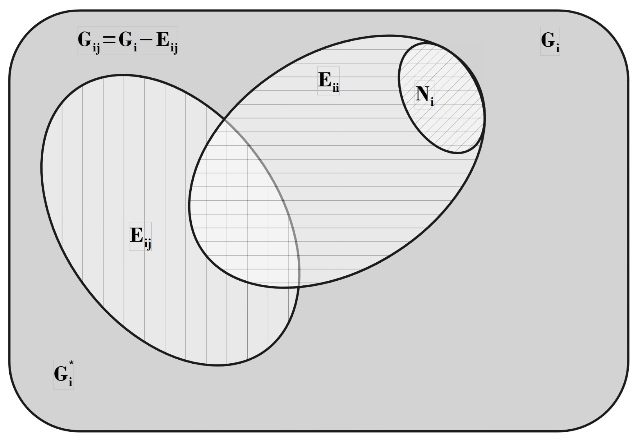
It is worth noticing that the fraction can also be interpreted as the probability for a state of species i being non-excluded by particles of species j. Accordingly, represents the probability that a state of species i is simultaneously non-excluded by all species. Then, assuming in a first approximation that the pairs cross-exclusion events are independent, can be written as
where the functions are given by Equation (311).
In order to finally obtain as defined in Equation (306) from in Equation (312), and by denoting , it is required that satisfies and 13, where is the maximum occupation of species i when other species are at densities .
Introducing normalization constants and so that , and using , the boundary conditions are fulfilled by setting and . Then, the density of states reads
for , with given by Equation (311).
The Helmholtz free energy for the generalized mixture on spatially correlated states can now be computed from Equations (311), (313), and (306), providing the full thermodynamic behavior.
As will be discussed in the applications, the quantities can be predetermined in model systems such as k-mer mixtures on regular lattices from the system symmetry 14.
Finally, note that the set cardinalities in this derivation do not depend on specific microstates, but represent effective values for configurations at equilibrium minimizing the Helmholtz free energy at given T and V (i.e., given ).
The parameters are consistently determined from particle and lattice properties (size, shape, connectivity), and from thermodynamic boundary conditions by generalizing the analysis developed introduced for single-component systems [18] .
6.2. Mixtures Statistical Thermodynamics
From the Helmholtz free energy in Equation (306) we derive the density dependence of the chemical potential ,
consequently, from Equations (306) and (314),
where, for the sake of shortness, the explicit dependence of on is implicit in Equation (315) and . We write Equation (315) more conveniently as
with for which straightforwardly give the chemical potentials as a function of the species state occupation numbers , or specie’s density. The Equation (316) also represents a system of s-coupled equations whose solutions are the species occupation numbers for given chemical potentials .
By defining , Equation (316) can be rewritten as
or
which are the coupled equations within the statistics from which the equilibrium distributions can be determined.
It is worth noticing that Equation (318) reduces to Wu’s distribution for fractional exclusion statistics [15] when the species’s states are spatially uncorrelated. An alternative picture of what the Wu’s limiting case of spatially uncorrelated species’s states means here is that the numbers of self-excluded and cross-excluded states per particle are constants in Wu’s formalism [15] and density dependent in statistics.
6.3. State Exclusion Spectrum Functions: Determination of Exclusion Correlation Parameters
This section is devoted to determining the parameters from the thermodynamic limits of the exclusion spectrum functions, which quantify the average cumulative number of self-excluded and cross-excluded states per particle as functions of the occupation numbers . For model systems where both the size/shape of the particles and the spatial distribution of accessible states (e.g., the lattice geometry) are known, the values of can be determined within the statistics framework, enabling a complete thermodynamic description.
Assume that species in volume V can exchange particles with a reservoir at temperature T and chemical potentials . The time evolution of the mean occupation number follows:
where and denote the average fractions of empty and occupied states for species i, and , are the respective transition rates. At equilibrium, and the detailed balance condition gives . Since , then from Equation (316), we have Substituting from Equation (316), we obtain:
The generalized exclusion spectrum function is defined as , which measures the total average fraction of states excluded to a particle of species i at given occupations (including both self- and cross-exclusion). The cumulative number of excluded states of species i per particle of species j, i.e., the spectrum function , is defined as:
Additionally, the rate of excluded states per particle due to self- or cross-exclusion is given by the partial derivatives:
Let , , and , which yield:
Solving for the self-exclusion parameters ,
where refers to Lambert function (see Section 5.4).
For the cross-exclusion case
For uncorrelated states (), and , as in Wu’s formalism [15].
The exclusion spectrum functions are related to density and chemical potential through
Although this formulation links measurable thermodynamic quantities to exclusion spectrum functions, its experimental application, especially for mixtures, requires further work. In dicussing applications further on in Section 7.8, we illustrate how and can be computed for k-mers on a square lattice, their behaviour through the k-mers transitions and usefulness display and characterize the order of transitions.
6.4. The k-Mers Problem as a Mixture Model: Basic Definitions
Preliminarly to applications of statistics, which we will discuss in Section 7.8, we introduce here the problem of k-mers on square lattice of M sites rationalized as a mixture of two differently oriented species.
As discussed in Section 5.5, the adsorption of straight rigid k-mers on square lattices for exhibits two distinct phase transitions: (1) a continuous, entropy-driven isotropic-to-nematic (I-N) transition occurring at intermediate surface coverage [96,101,104], and (2) a nematic-to-isotropic (N-I) transition taking place at densities approaching lattice saturation [106].
In Ref. [18] k-mers on the square lattice has been modeled as a binary mixture of species aligned along the horizontal () and vertical () lattice directions, denoted as species 1 and 2, respectively. Both species occupy k consecutive lattice sites along their respective directions. According to our definitions: , , , and . The exclusion parameters are , and the saturation values satisfy .
From Equation (313), the saturation occupations under coexistence are:
The self-exclusion at infinite dilution is , leading to . For cross-exclusion, each k-mer excludes states orthogonal to its direction, of which are shared. Thus, .
Using Equation (326), the cross-exclusion correlations are
where is the Lambert function. Solving this yields for , for , for , and for .
Based upon this elementary definition of the mixture parameter, the thermodynamic and exclusion functions in the statistics, a much comprehensive treatment of the problem is given in Section 7.8, leading to the entropy surface, equilibrium paths, density branches, order parameters, transition critical points and state exclusion spectrum are obtained for various values of k.
7. Applications
In the present section, we analyze the scope and limitations of the theoretical models developed in previous sections by comparing them with Monte Carlo simulations and experimental data available in the literature.
7.1. Two-Dimensional Adsorption: Comparison Between Theory and Monte Carlo Simulations
In this section, adsorption isotherms are calculated for the theoretical models introduced in Section 3 (, , , , and ) and compared both among themselves and against Monte Carlo simulations performed within the grand canonical ensemble framework [see Section 8]. These comparisons are conducted for honeycomb, square, and triangular lattices.
Monte Carlo simulations were carried out on honeycomb, square, and triangular lattices of size , with , and 150, respectively, using periodic boundary conditions. This lattice size ensures that finite-size effects are negligible. In addition, MCSs.
We begin by discussing some fundamental features of the adsorption isotherms. Figure 24 presents a comparison between the exact adsorption isotherm for monomers and the simulated isotherms for dimers on honeycomb, square, and triangular lattices. As observed, the particle–vacancy symmetry, which holds for monoatomic adsorbates, breaks down when . Furthermore, while the dimer adsorption isotherms appear similar across the different lattice types, the curves shift to lower values of as the connectivity increases. In other words, for a given value of , the equilibrium surface coverage rises with increasing . This behavior can be explained using the following relation:
which is valid for linear k-mers at low concentrations [see Equation (149)]. As the chemical potential increases, this effect diminishes, and consequently, the slope of the isotherms decreases with increasing .
We now consider the case of linear adsorbates larger than dimers. For honeycomb lattices, k-mers adsorb as described in Section 3.1.1. When a site is selected, there are six possible equilibrium orientations for a single k-mer () at extremely low coverage, resulting in a total number of k-uples equal to (i.e., ), as is also the case for triangular lattices.
Based on these conditions, extensive simulations were conducted for linear adsorbates with k ranging from 2 to 10. As illustrative examples, Figure 25(a), Figure 26(a), and Figure 27(a) compare simulation isotherms with theoretical predictions for 6-mers on honeycomb, square, and triangular lattices, respectively. In all cases, the theoretical models agree well with simulations at low coverages, but deviate significantly as the surface coverage increases.
The discrepancies between simulation and theory can be quantified by the percentage reduced coverage, defined as [73]
where () represents the coverage obtained by using MC simulation (analytical approach). Each pair of values () is obtained at fixed .
Figure 25b, Figure 26b, and Figure 27b show how varies with surface coverage for the different lattice types. The performance of each theoretical model is as follows: the model (dashed line) shows very good agreement with simulation results, with minimal discrepancies. Both the (dash-dot-dot line) and (dash-dot line) models tend to underestimate the coverage across the entire range. The model (dotted line) performs poorly at intermediate coverages but improves at high coverages. With respect to lattice connectivity, the accuracy of and improves as decreases, while the opposite trend is observed for and . The behavior of the and models supports the formulation of the semi-empirical () isotherm (solid line) given in Equation (155). This trend is also illustrated in Figure 28, Figure 29, and Figure 30, which show the percentage reduced coverage for the model as a function of concentration for various values of and k.
To better interpret the data shown in Figure 28, Figure 29 and Figure 30, we consider two summary metrics: (1) the average absolute difference between simulation and theoretical coverage, ; and (2) the maximum value of the percentage reduced coverage, . These metrics are presented in Figure 31. Several conclusions can be drawn: (i) theoretical models generally perform better on square lattices; (ii) both and remain nearly constant for k values between 2 and 8; and (iii) both quantities increase for . Finally, since the values of remain below , the model can be considered a reliable approximation for describing multisite occupancy adsorption, at least for the k values analyzed here.
7.2. Two-Dimensional Adsorption of Binary Mixtures: Comparison Between Theory and Monte Carlo Simulations
In this section, we analyze the main characteristics of the theoretical approximations developed in Section 3.3 in comparison with MC simulation results and experimental data.
We consider a gas mixture composed of rigid rods of lengths k and l, with each component present in equal molar fraction in the gas phase. Adsorption occurs on a regular, homogeneous lattice with connectivity (square lattice) and 6 (triangular lattice). The parameters used in the HPTMC simulations (see Section 8.3) were: , and MCSs. For simplicity, we assume the standard chemical potentials are zero and that the equilibrium constants for all species.
The partial adsorption isotherms for , , and two values of are shown in Figure 32(a) and Figure 32(b), respectively. Symbols denote MC simulation data, while the lines represent various theoretical approaches as indicated.
A characteristic feature observed in binary mixtures of polyatomic species is evident in both figures: at higher pressures, the smaller species are displaced by the larger ones. This phenomenon, known as adsorption preference reversal (APR), arises from entropic competition between adsorbed species. A detailed investigation of the APR effect, focusing on the impact of molecular size difference, is presented in Section 7.4.
In Figure 32(a), the most significant discrepancies between simulation and theoretical predictions occur in the partial adsorption isotherm of the larger species. As clearly shown in Figure 32(b), the magnitude of these deviations depends on the level of approximation used in evaluating [11].
To quantitatively assess the agreement between simulation and analytical results, we use the reduced coverage error defined in previous section [73],
where represents the value of the total coverage obtained by using the MC simulation (analytical approach). Each pair (, ) corresponds to the same value of pressure P.
The results obtained from Equation (332) are shown in Figure 32c,d. In Figure 32c, better agreement is observed at surface coverage above , where only dimers are present, a case where all theoretical models perform well [16]. Conversely, for larger adsorbates, classical approaches fail to accurately describe the adsorption behavior across the entire range of coverage, as illustrated in Figure 32d. In contrast, the approximation yields satisfactory results, with errors remaining below in both cases.
The same analysis presented in Figure 32 is repeated for triangular lattices, with the corresponding results shown in Figure 33. In most cases, the error increases with lattice connectivity. However, the approximation consistently yields an error below , indicating that it is a highly reliable method for modeling binary mixture adsorption with multisite occupancy, at least for the molecular sizes considered in this study.
To complete our analysis, we examine partial isotherms for mixtures with varying sizes of l, keeping fixed. For each pair (k, l), the discrepancies between theoretical predictions and simulation results are assessed using the average error across the full coverage range, defined as
where R is the total number of isotherm points (or the number of replicas, as described in Section 8.3).
Figure 34 illustrates the dependence of on the size of the l-mers and the lattice geometry for the various theoretical approaches evaluated in this work. As shown, increases monotonically with l, indicating that the divergence between MC simulations and analytical models becomes more significant for larger adsorbates. In contrast, the error associated with the approximation remains nearly constant, around for square lattices and for triangular lattices. This excellent agreement across all values of l highlights the robustness of the method and underscores the importance of accurately computing the correction function [Equation (187)] for understanding the adsorption behavior of rigid rod mixtures.
Finally, to evaluate the applicability of the proposed model, we analyzed experimental data extracted from Ref. [116]. Specifically, adsorption isotherms of hydrocarbon mixtures—methane–ethane and ethane–propylene—on activated carbon (AC-40) at C were examined using the adsorption model introduced in this work. Since the experimental data were reported as adsorbed amount (in ) versus pressure (in mmHg), the theoretical isotherms were reformulated in terms of pressure P and adsorbed amount g to enable direct comparison and fitting.
Assuming equilibrium between the adsorbed phase and an ideal gas-phase mixture, the chemical potentials were related to the system pressure and molar fractions. Additionally, the coverage was defined as , where represents the maximum adsorption capacity of the surface.
Following a common approach in the literature, a “bead segment” chain model was employed in which each CHn group (bead) occupies one adsorption site on the surface. Accordingly, each hydrocarbon species Cm was modeled as a rigid rod of length [117].
Within this framework, the experimental isotherms for methane–ethane and ethane–propylene mixtures at C and varying molar fractions were fitted using a single value of and temperature-dependent equilibrium constants as adjustable parameters. The results of the fitting procedure are shown in Figure 35, and the corresponding parameter values are summarized in Table 1. A very good agreement is observed between experimental data (symbols) and theoretical predictions (solid lines).
While a more extensive analysis of experimental adsorption isotherms is still needed, these results suggest that the theory provides a promising and accurate framework for describing the adsorption thermodynamics of interacting polyatomic species.
7.3. Two-Dimensional Adsorption of Interacting k-Mers: Comparison Between Theory and Monte Carlo Simulations
In this section, we analyze the main features of the thermodynamic functions derived from the models presented in Section 4.1 (Bragg-Williams Approximation, ) and Section 4.2 (Quasi-Chemical Approximation, ), in comparison with Monte Carlo simulation results for a lattice-gas of interacting dimers on honeycomb, square, and triangular lattices. 15
As in Section 7.1, simulations were conducted on honeycomb, square, and triangular lattices of size , with , 144, and 150, respectively, using periodic boundary conditions. Moreover, the lattice size L was carefully selected to avoid perturbation of the adlayer structure.
Representative adsorption isotherms obtained from Monte Carlo simulations in the grand canonical ensemble (symbols), along with their comparison to the (solid lines) and (dashed lines), are shown in Figure 36, Figure 37, and Figure 38 for honeycomb, square, and triangular lattices, respectively.
For attractive interactions [Figure 36a, Figure 37a, and Figure 38a], as temperature decreases, a first-order phase transition occurs, evidenced by the discontinuity in the simulated isotherms and the appearance of characteristic loops in the theoretical curves. This behavior, experimentally observed in many systems [80], corresponds to a low-coverage lattice-gas phase coexisting with a higher-coverage “lattice-fluid” phase. The lattice-fluid can be considered as a diluted version of the registered phase where all lattice sites are occupied except for some vacancies.
This two-dimensional gas-to-liquid condensation closely resembles that of a monomeric lattice gas with attractive interactions. However, for k-mers, the particle-vacancy symmetry (valid for monomers) is broken, resulting in adsorption isotherms that are asymmetric with respect to .
In the case of repulsive interactions [Figure 36b, Figure 37b, and Figure 38b], the isotherms exhibit more complex features due to the formation of ordered structures in the adsorbed layer. These ordered arrangements are indicative of subcritical behavior, where continuous phase transitions occur from disordered to ordered phases [118,119]. At high temperatures, isotherms remain featureless, but at low temperatures, they display distinct steps corresponding to the emergence of ordered phases. The specific form of these steps depends strongly on the lattice connectivity. As the chemical potential increases and the surface coverage spans from 0 to 1, two ordered phases are typically observed: (1) a low-coverage ordered phase (LCOP), characterized by site occupancies of , , and for honeycomb, square, and triangular lattices, respectively; and (2) a high-coverage ordered phase (HCOP), with site occupancy across all three geometries. Snapshots of the LCOP [part a)] and HCOP [part b)] configurations for each lattice type are presented in Figure 39, Figure 40, and Figure 41. For a detailed discussion of these phases, refer to Refs. [118,119].
Under attractive interactions, both theoretical models yield qualitatively similar results, and the isotherms from and are nearly indistinguishable. However, it is known that isotherms derived from fundamentally different approximations can appear deceptively similar [67]. To better assess the accuracy of each model, we use the absolute error in the chemical potential, , which is defined as
where () represents the chemical potential obtained by using MC simulation (analytical approach). Each pair of values (, ) is obtained at fixed .
As an example, Figure 42(a) presents for three representative attractive interaction strengths: squares for , triangles for , and circles for . Solid and open symbols correspond to and results, respectively. In all cases, outperforms .
The corresponding analysis for repulsive interactions is shown in Figure 42b, which includes (squares), (triangles), and (circles). Again, solid and open symbols represent and , respectively. Here, differences between the two models are both quantitative and qualitative. While fails to predict any ordered structures, captures the formation of a pronounced plateau at low temperature. This critical coverage, , appearing between the LCOP and HCOP, depends on both lattice geometry and adsorbate size. The adsorbate configuration at can be interpreted as a mixture of LCOP and HCOP phases [see part (c) in Figure 39, Figure 40, and Figure 41].
The curves in Figure 42 correspond to a honeycomb lattice. However, the behavior of for square and triangular lattices is very similar (data are not shown here for sake of simplicity).
To quantify the overall deviation between theory and simulation across the full coverage range, we define the integral error as:
Figure 43 shows for all lattice geometries and a broad range of values. Several key conclusions can be drawn: In all cases, provides a significantly better fit to the simulation data than . This is particularly true for repulsive interactions, where shows large discrepancies, while remains the simplest yet effective model for describing multisite occupancy adsorption. The value of increases with lattice connectivity. This may be attributed to a loss in accuracy of as increases [73]. There exists a broad range of interaction strengths () for which matches the simulation data extremely well. Notably, most surface science experiments fall within this range of interaction energies.
Therefore, not only represents a clear improvement over the in modeling k-mer adsorption but also provides a solid theoretical framework and compact expressions for the interpretation of thermodynamic adsorption data of polyatomic species—such as alkanes, alkenes, and other hydrocarbons—on regular surfaces.
7.4. Application of to the Adsorption of and in Zeolites 13X and 5A: Determination of the Adsorption Configuration
One interesting application of the theoretical framework presented in Section 3.2.2 on a lattice gas model involves the interpretation of experimental adsorption isotherms for propane [120] and oxygen [121,122] in 13X and 5A zeolites, as well as in simulation-based systems. In our approach, we employed Equation (125) under two main assumptions: since constant, if a single molecule has m distinct ways to adsorb per lattice site at zero coverage, then the presence of an adsorbed k-mer, occupying sites, effectively excludes states from being accessible to other molecules [thus, ]; and the energetic contribution from adsorbate-adsorbate interactions is accounted for using a mean-field approximation, as described in Section 4.1. This analysis highlights the physical interpretation of the parameters g and a, linking them to the spatial configuration of adsorbed molecules and the geometric structure of the surface.
Because the experimental data are presented as adsorbed volume v, against pressure p, we rewrite Equation (125) in the more convenient form:
where ( is the volume corresponding to monolayer completion); ; is the equilibrium constant ; and is the mean-field term. In addition, can be associated with the isosteric heat of adsorption .
Figure 44 presents the adsorption isotherms of propane () in zeolite. Solid lines represent theoretical predictions using the model, while symbols show experimental data from Ref. [120]. Following conventional modeling, alkane chains are treated as "bead segments," where each methyl group corresponds to one adsorption site. Accordingly, propane is modeled as a trimer with . Given that the propane molecule () is relatively large compared to the cavity diameter (), it likely adsorbs along a preferred orientation. Otherwise, accommodating 5–6 molecules per cavity would be unfeasible. We thus assign (with and , mimicking a 1D configuration). The best fit to the experimental data over the full temperature and pressure range was obtained by simultaneously optimizing , and w (see Table 2).
Consistent with experimental findings, the resulting is slightly under 6 molecules per cavity. A value of suggests that some molecules may partially span across the cavity windows. Regarding the lateral interaction parameter w, its ratio to the known liquid-phase interaction energy for propane is about , indicating that each molecule interacts, on average, with 2.5 neighbors at full coverage. This supports the approximation of a quasi-one-dimensional system.
Figure 45 also shows strong agreement between theory and experimental data for a system with non-monotonic adsorption behavior. In this case, the derivative of the adsorbed volume with respect to pressure was fitted, again yielding excellent correlation.
To quantify model accuracy, we define the deviation D as the average relative discrepancy (in percent) between theoretical () and experimental () data:
where i runs over the total set of data.
For propane on 13X, D was found to be (Table 2), which is within the bounds of experimental error, underscoring the robustness of the approach. In contrast, a previous model from Ref. [120] required eight parameters to describe similar systems. Here, the complexity of polyatomic adsorption is captured through a single, physically meaningful parameter g, reflecting the spatial configuration of the adsorbate.
We now turn to the oxygen adsorption isotherms in 5A zeolite, shown in Figure 46. Symbols denote experimental measurements, while lines indicate theoretical curves from Equation (336). Experimental data were taken from two different sources in the literature, from Miller et al. [121] and Danner et al. [122]. In the first set of data (empty symbols) [121], the amount adsorbed was measured in units of the number of molecules per cavity. In the other case (full symbols) [122], the amount adsorbed was reported in units of per of adsorbent.
Figure 46.
Adsorption isotherms for adsorbed in zeolite. Empty and full symbols correspond to data from Refs. [121,122], respectively. Lines correspond to the adsorption isotherm function of Equation (336).

The fitting process involved two steps: based on previous numerical simulations [123], we fix ( and ). Under these considerations, analytical isotherms in Figure 46 were obtained by multiple fitting the set of parameters , and w as in Figure 44. The value obtained for w is in excellent agreement with the simulational calculation of w in Ref. [123]. With respect to , it was not possible from the work of Razmus et al. [124] to estimate in order to compare with the one from Equation (336). However, was independently validated through a second stage of fitting; the values of g, and w arising from were fixed. Then, , set as to fit the experimental isotherm measured by Danner et al. [122], agrees with the monolayer volume reported in Ref. [122]. The deviation between experimental and fitting curves was (see Table 2). Based in the consistency of this analysis, appears to adsorb flat with two possible orientations on a two-dimensional layer defined by the cavity’s inner surface.
The isosteric heat of adsorption for both systems was derived from the slope of the plot of versus , as shown in Figure 47. The results, which are presented in Table 2, align well with reported experimental values for propane in 13X [120] and oxygen in 5A [124].
Finally, in order to illustrate the applicability and versatility of to describe systems more complex than the one in the experiments analyzed here, we show in Figure (Figure 48) the fit (solid lines) to numerical isotherms (symbols) of dimers, flexible trimers and flexible tetramers adsorbed flat on a square lattice. Solid lines represent the best fitting to computer experiments in the crudest approximation [constant, Equation (125)] to the general isotherm of Equation (124). The values obtained for g in all cases are very consistent to the ideal value . It is worth mentioning that, at this elementary degree of approximation is already more accurate than the classical Flory’s theory [6] of adsorbed chains as well as the multisite-adsorption approaches of Refs. [20,33].
For the case of dimers, the inset in Figure (48) shows a comparison between the configurational entropy per site, s, versus coverage from simulation and the corresponding ones obtained from [being and ] for different values of g. As it was calculated for the isotherm, the best fit corresponds to (solid line). The three curves in dashed (dotted) lines correspond to increments (decrements) of , and with respect to . As it can be clearly visualized, small variations of g provide notable differences in the entropy curves. Thus, the statistical exclusion parameter g results highly sensitive to the adparticle’s spatial configuration. The more compact the configuration of the segments attached to the surface sites the smaller g. For instance, g may vary from () for straight trimers (tetramers), to () for flexible trimers (tetramers).
In summary, the study presented in this section demonstrates how the concept of statistical exclusion () serves as a powerful tool to quantify the entropy associated with polyatomic adsorption, effectively capturing both the configuration and interaction of adsorbates. Furthermore, Equation (124) lays the groundwork for analyzing configurational changes as a function of coverage [through configurational spectroscopy ] from thermodynamic data. Overall, offers a compact and insightful framework for interpreting adsorption phenomena, from simple gases to complex hydrocarbons on structured surfaces.
7.5. Adsorption of Methane-Ethane Mixtures in Zeolites: Reversal Adsorption Phenomena
The adsorption of molecular mixtures presents a significantly greater challenge than that of pure components, both experimentally and theoretically. While the number of adsorbed molecules in a pure gas system can be accurately determined by measuring the weight gain of the adsorbent sample, studying mixtures requires additional experimental techniques to determine the composition of the adsorbed phase. This complexity is one of the primary reasons for the scarcity of experimental data on the adsorption of polyatomic mixtures.
Nonetheless, several simulation studies have investigated the behavior of hydrocarbon mixtures [125,126,127,128,129,130,131,132]. A particularly striking phenomenon has been observed in methane–ethane mixtures [125,126]: at low pressures, the adsorbed phase is dominated by ethane, but as pressure increases, methane gradually displaces ethane. This inversion in adsorption preference has also been reported in mixtures of linear hydrocarbons adsorbed in silicalite [127,128,129,130,131,132], as well as in carbon nanotube bundles [133] and metal-organic frameworks [134]. In all these cases, selectivity shifts from favoring the larger molecule at low pressure to favoring the smaller one at higher pressure—a behavior known as Adsorption Preference Reversal (APR) [51].
From a theoretical standpoint, understanding the origin of APR is not straightforward. Within the framework of single-site adsorption (where each molecule occupies a single lattice site), studies by Ayache et al. [51] and Dunne et al. [52] have shown that competition between species under repulsive lateral interactions can cause one component to replace the other in the adsorbed phase. In their approaches, Ayache et al. [51] used a mean-field approximation, while Dunne et al. [52] performed exact calculations. However, hydrocarbon molecules adsorbed on solid surfaces should be regarded under the light of a multisite-adsorption model, in order to properly account for the effects of configurational entropy (k-mer size and flexibility) on the thermodynamics of the adlayer. Entropic effects arising from differences in molecular structure and density are expected to drive a range of complex behaviors and phase transitions in such systems.
Understanding how molecular size and structure affect the thermodynamic properties of the adsorbed layer is of fundamental importance in statistical physics. Furthermore, developing accurate theoretical descriptions of these systems has practical relevance in designing and optimizing separation processes in petrochemical applications. In this context, we present the first exact model for adsorption of molecular mixtures in zeolites that accounts for multisite occupancy. Using a rigorous statistical thermodynamic approach, we analyze mixtures of s-mers and k-mers (molecules occupying s and k lattice sites, respectively) on one-dimensional substrates. Our results reveal that the APR phenomenon emerges naturally from differences in molecular size (i.e., number of occupied sites) between the two species.
Following the line of Ref. [51], we start calculating the parameter , which is obtained from the equilibrium equations [Equations (33) and (34) in Section 2.1.2]:
In order to understand the basic phenomenology, we consider in the first place a monomer-monomer mixture (), with equimolar amounts of each kind of molecules in the gas phase (). Under these conditions, Equation (338) can be written as:
In this case, const. Accordingly, the partial adsorption isotherms corresponding to the species s and k do not intersect and the APR phenomenon does not occur. This situation is reflected in Figure 49, where an equimolar monomer-monomer mixture has been studied for and . The inset shows a similar analysis, where the values of the adsorption energies per particle were taken from Ref. [51]: ( J and T=250 K) and ( J and T=250 K). In addition, the values of and were obtained by using Equation (168) (Section 2.1.2) with () equal to the molecular mass of methane (ethane). Thus, uma, uma (where 1 uma kg) [135] and, consequently, and .
The results presented in Figure 49 align with earlier studies on monomer–monomer mixtures [51], where the occurrence of APR required introducing a complex set of lateral interactions.
We now turn to the more general case of an equimolar mixture composed of s-mers and k-mers. As indicated by Equation (338), when both species have the same size (), the individual adsorption isotherms do not intersect, and the resulting curves resemble those observed in Figure 49.
However, when , the system exhibits a broader range of behaviors that depend on both the value of the interaction parameter A and the size relationship between the two species. Without loss of generality, we consider the case where . In evaluating the role of A, we rely on two key physical assumptions regarding the adsorption of linear alkanes: the heats of adsorption are attractive and increase (in absolute value) linearly with the length of the hydrocarbon chain. It is important to emphasize that these are not merely theoretical assumptions—they reflect well-established experimental findings on the energetics of alkane adsorption in zeolites, supported by extensive literature evidence [117,136,137,138].
Under these considerations, the argument of the exponential in Equation (338) is negative, A varies between 0 and 1 and there exists a value of coverage, (), at which the partial isotherms coincide () and, consequently, the APR phenomenon occurs. The value of can be obtained from Equation (338) by simple algebra:
The crossing point separates two adsorption regimes. Thus, for , is larger than . This tendency is reverted for , where is larger than . Then, the existence of the point is directly related to the displacement of the species k by the species s, and, consequently, to the presence of APR phenomenon.
This behavior is clearly illustrated in Figure 50, which examines a monomer–dimer mixture ( and ) with equal concentrations of each species in the gas phase. The parameter values for , , and are the same as those given in the inset of Figure 49. This monomer–dimer case is particularly insightful because: it represents the simplest model of binary adsorption involving species of different sizes; it captures the essential characteristics of multisite-occupancy adsorption; and it serves as a useful model for interpreting experimental adsorption of methane–ethane mixtures in silicalite. Following a widely used approach, we adopt the bead-segment model, where each methyl group is represented by a single unit (or “bead”) equivalent in size to one adsorption site. Within this framework, methane and ethane are modeled as and , respectively.
Given that ethane molecules possess a stronger affinity for the surface (higher adsorption energy), they adsorb preferentially at low pressures. However, as pressure increases, adsorption of the smaller methane molecules becomes more favorable, eventually displacing the previously adsorbed ethane. As a result, the partial isotherms intersect at a critical coverage , indicating the occurrence of APR phenomenon. In this specific case, .
The exact results presented here offer a significant contribution to understanding the APR mechanism, demonstrating that it naturally arises from size disparity (or more precisely, the number of occupied sites) between different adsorbed species. It’s worth highlighting that in earlier theoretical treatments, such as the monomer–monomer model presented in Ref. [51], reproducing APR required a highly parameterized model involving six variables (adsorption energies for methane and ethane, pairwise interaction energies among methane–methane, methane–ethane, and ethane–ethane, plus temperature). This complexity led to poorly constrained parameters and only qualitative conclusions. In fact, extremely small changes in parameter values (much smaller than typical experimental uncertainties) produced vastly different predictions. For example, a mere 5 percent change in ethane’s adsorption energy could determine whether APR appears or not in the model of Ref. [51].
Supporting this point, Equation (340) demonstrates that APR can emerge solely due to size asymmetry (), even in the absence of any energetic contributions or lateral interactions ( and ). This reveals that introducing complex lateral interactions in previous models may be seen as an artificial or effective way to account for purely geometric or steric effects through energetic means.
In summary, this study leads to two key conclusions: the entropic effects arising from the non-spherical nature of polyatomic adsorbates play a crucial role in surface phenomena and cannot be neglected in comparison with monoatomic adsorption, and failing to incorporate the polyatomic nature of adsorbates into thermodynamic models can lead to a serious misinterpretation of experimental data, particularly regarding phenomena like APR.
7.6. Alkanes Adsorbed in Carbon Nanotubes Bundles: Surface Area Characterization
The multilayer adsorption theory for polyatomic molecules, discussed in Section 2.1.3, is utilized here to evaluate the surface area of a HiPco single-walled carbon nanotube (SWCNT) sample. This analysis is based on adsorption isotherms obtained using a series of four alkanes—methane through butane.
The SWCNT sample analyzed in this study was procured from Carbon Nanotechnology Inc. (CNI). No post-processing was applied beyond evacuating the sample under vacuum (better than Torr) for 72 hours before each measurement cycle. Although the purification method used by the manufacturer may have opened some nanotube ends, these openings were effectively sealed by chemical groups introduced during that same process [139]. To unblock these caps, heating to at least 650 K under vacuum is necessary [140,141], a procedure not undertaken in this work. As a result, internal adsorption was excluded, and the sample effectively behaved as a non-porous substrate. Adsorption primarily occurred on the external surfaces of nanotube bundles and, to a lesser extent, on large-diameter, defect-related interstitial sites [142,143].
The isotherms were recorded using a custom-built volumetric adsorption setup [144]. Low temperatures were achieved using a helium closed-cycle refrigeration system, and temperature regulation was maintained with two controllers. Pressure measurements were conducted using three capacitance manometers, with upper limits of 1, 10, and 1000 Torr, respectively. These gauges were housed in the room-temperature gas-handling system. Data acquisition and gas dosing were managed by a LabView-based program developed in-house. All gases employed were of ultra-high purity, sourced from Matheson Gas.
To determine the surface area, we calculated the product of the molecular area of the adsorbate [145,146,147] and the monolayer capacity of the substrate. The monolayer capacity was derived from experimental adsorption isotherms using two approaches: the BET method [54,60] and the point B method [148,149]. The specific surface area was then calculated by dividing the total surface area by the sample’s mass.
The point B method involves plotting the adsorption isotherm as adsorbed amount versus pressure on a linear scale. Initially, coverage increases steeply with pressure, eventually reaching a pronounced inflection point. Beyond this point, coverage increases more gradually and linearly, until multilayer adsorption begins. Point B is identified as the lowest pressure at which a linear extrapolation aligns with this intermediate linear region between the completion of the first layer and the start of the second [148,149]. The coverage at point B corresponds to monolayer completion, as illustrated in Figure 51. Generally, this method yields a slightly higher monolayer capacity than the BET equation.
Figure 52 shows the isotherms obtained for the HiPco nanotube sample using methane, ethane, propane, and butane. Different temperatures were used for each alkane due to their differing adsorption energies. Methane requires low temperatures where other alkanes exhibit vapor pressures too low for reliable measurement in our setup [150,151]. Conversely, the higher temperatures suitable for measuring butane adsorption produce pressures for methane that are too high to resolve the monolayer region effectively [151].
To ensure comparability across different gases, isotherm temperatures were scaled by each adsorbate’s bulk critical temperature (), aligning the scaled temperatures across the data sets.
Table 3 compiles the molecular areas of the alkanes used. They were obtained from published neutron scattering results for alkane films adsorbed on graphite [145,146,147].
Figure 53 presents plots of the linearized BET equation for the four different adsorbates used. The linearized BET equation is
In this context, P refers to the pressure at a specific point on the adsorption isotherm, is the saturated vapor pressure of the adsorbate at the isotherm temperature, n denotes the number of molecules adsorbed at pressure P, represents the monolayer capacity of the substrate, and C is a constant that reflects the interaction strength between the adsorbate and the substrate.
The BET equation is typically applied over a range of relative pressures from approximately 0.05 to 0.3 [54,60,149]. This is the pressure range used for plotting the isotherm data in Figure 52, which yielded the results shown in Figure 53.
Figure 54 displays the specific surface area values for the HiPco nanotube sample, as determined using both the point B method and the BET equation for different adsorbates. Notably, both methods reveal the same trend: as the molecular length of the adsorbate increases, the specific surface area calculated for the same sample decreases. Within the range of molecule sizes examined, this decrease is approximately for each method.
In an earlier study, we measured the specific surface area of a SWCNT sample using several spherical adsorbates (neon, argon, methane, and xenon) and found that the value was essentially independent of the size of the adsorbate [152]. That analysis employed the point B method to determine monolayer capacity. These results differ markedly from the findings reported here for the linear alkane series (methane through butane). The key distinction lies in molecular geometry: unlike the spherical adsorbates used previously, the alkanes are linear, which enhances their tendency for multisite occupancy during adsorption.
We now proceed to analyze the experimental data using the theoretical framework for multilayer adsorption of polyatomic molecules, as developed in Section 2.1.3 and Section 3.4. The model outlined in Section 2.1.3 will be referred to hereafter as the "modified BET model," or simply the MBET model. As previously mentioned, in the one-dimensional (1-D) case, the MBET equation reduces to the standard BET equation when considering monomer adsorption (). The explicit expression derived for the adsorption of dimers () in 1-D within the MBET framework is given by:
The variables appearing in Equation (342) carry the same meaning as those defined in Equation (341). Equation (342) is applicable for determining the monolayer capacity and specific surface area in the case of ethane adsorption, where ethane molecules can be effectively treated as dimers. Unlike the standard BET equation, the MBET expression for dimers is nonlinear. When applied to ethane, the MBET model yields a larger surface area than the value obtained using the BET equation on the same dataset. Notably, the MBET model for dimers involves only two adjustable parameters—the same number as in the BET formulation.
As previously mentioned, for systems with in two dimensions (2-D), no exact analytical expressions exist for adsorption isotherms, i.e., for the fractional coverage n as a function of the relative pressure . To address this challenge, we adopted two different strategies to extract monolayer capacity from experimental data:
- (1)
-
In this first approach (procedure A), we used the one-dimensional MBET equations for all four adsorbates to account for the linear geometry of the molecules. For methane, we employed the standard BET equation, which corresponds to the MBET expression for monomers. For ethane, we applied the exact 1-D MBET formula for dimers [Equation (342)]. For propane and butane, we utilized the same dimer equation but adjusted its parameters to fit the experimental data in the low-pressure, low-coverage regime—specifically, the same region typically used in BET analysis.Using Procedure A, the calculated specific surface areas for ethane, propane, and butane were consistently higher than those obtained using the BET method. In addition to producing improved results, this method remains relatively straightforward to implement.However, we also observed a consistent trend: as the length of the alkane chain increases, the derived specific surface area decreases. This behavior is illustrated in Figure 6, which includes data obtained from both this and other approaches.Although not perfect, the results from Procedure A represent a clear enhancement over the standard BET approach.
- 2)
-
The second strategy (procedure B) involved fitting the isotherm data for all four adsorbates to the approximate MBET expression developed for the two-dimensional case [Equation (209) in Section 3.4]In this formulation, is a constant that reflects both the interaction strength between the adsorbate and the substrate, as well as the connectivity of the adsorption lattice. The parameter k denotes the number of units in the k-mer molecule.The experimental adsorption isotherms are fitted to this model using the appropriate k value for each adsorbate—1 for methane, 2 for ethane, 3 for propane, and 4 for butane—within the same low-pressure range typically employed for BET analysis. Figure 55 shows the fit obtained for butane, which demonstrates excellent agreement with the data; similarly accurate fits were achieved for the other three alkanes. The fits yield values for the monolayer capacity, , which are subsequently used to compute the specific surface area of the sample.
Figure 56 presents the key findings of this study. It shows the specific surface area values of the substrate calculated using the four methods discussed: the point B method, the BET equation, the 1-D MBET model (Procedure A), and the 2-D MBET model (Procedure B). These values are plotted against the number of carbon atoms in the alkane adsorbates used in the isotherm measurements. Among the four approaches, only the 2-D MBET model (Procedure B) produces surface area values that remain nearly constant across the range of adsorbates. In contrast, the other three methods show a decreasing trend in surface area with increasing alkane chain length.
This result has practical significance, as it offers a consistent approach for determining surface area using linear adsorbates. Specifically, the 2-D MBET model allows for surface area measurements with linear molecules that closely mirror the consistency typically achieved when using spherical adsorbates with the BET or point B methods.
From a more fundamental standpoint, our findings underscore the significance of the additional entropy contribution that emerges in monolayer films of linear molecules due to multisite occupancy.
To summarize, in this section we presented adsorption isotherm measurements for a series of four alkanes (methane, ethane, propane, and butane). These data were then used to estimate the specific surface area of a single substrate using four different methodologies: the traditional BET equation, the point B method, and two versions (1-D and 2-D) of a more recent model for the adsorption of linear molecules, known as the MBET method. Our key conclusion is that the 2-D MBET approach (procedure B) yields consistent surface area values across different linear adsorbates, in contrast to the other methods evaluated (point B, BET, or the 1-D MBET model), which do not show such consistency.
This result holds both practical and theoretical significance. Practically, it offers a reliable method for determining specific surface area using longer linear molecules, producing values that align well with those obtained from spherical adsorbates using the BET equation. This, in turn, enhances the comparability of results obtained for the same substrate across different types of adsorbates.
7.7. Crystal Growth from Aqueous Solution in the Presence of Structured Impurities
The process of crystal growth plays a vital role in both biological systems and industrial technologies. It begins with the formation of stable nuclei, followed by the gradual addition of atoms or molecules onto the crystal’s surface. These growth units—comprising atoms or molecules identical to those in the crystal—migrate from the bulk solution and attach to specific surface sites, eventually leading to the formation of macroscopic structures with well-defined surfaces.
It is well established that the adsorption of foreign atomic or molecular species, known as impurities, can significantly influence the rate of crystal growth [153,154,155]. This phenomenon has been widely utilized to control crystal morphology and to enhance the properties of crystalline materials, powders, and granulated substances. Understanding the mechanisms by which impurities exert their effects is therefore of considerable importance.
Numerous studies have explored the influence of impurities on both the growth rate and morphology of single crystals [156,157,158,159,160,161]. Theoretical models addressing this influence typically assume that impurities (ions, atoms, or molecules) adsorb at specific surface features such as kinks, steps, and terraces during crystal growth. Early theoretical efforts in this area were made by Bliznakov [162,163,164,165], who focused on impurity adsorption at step edges, and by Cabrera and Vermilyea [166], who considered adsorption on flat surface terraces. Experimental data on crystal growth rates have supported the predictions of these models [160].
In a key contribution, Davey and Mullin (DM) [167] developed a theoretical framework to describe how impurities affect the growth rate of crystals from aqueous solutions. Their model posits that impurity adsorption is limited to a thin layer adjacent to the crystal surface, and assumes no lateral or vertical interaction between adsorbed impurity molecules. Within this context, the velocity of step movement, V in the presence of impurities is given by:
where is the step velocity in the absence of impurities, and denotes the fraction of surface sites occupied by impurities. Consequently, reflects the proportion of available sites for the adsorption of pure growth units. As approaches 1, the surface becomes fully covered with impurity species, and crystal growth effectively halts.
The ability of an impurity to inhibit crystal growth is also believed to depend on factors such as its size, shape, and orientation—a phenomenon referred to as stereochemical effect. To incorporate these aspects, Kubota and Mullin (KM) [168] proposed an improved kinetic model. Their approach considers impurity adsorption along step edges and introduces a parameter, , representing the efficiency of impurity blockage. The step velocity in this model is given by:
This equation shows that the overall impact of impurities on growth rate is governed by two factors: the surface coverage by impurities () and the effectiveness of each adsorbed molecule () in hindering growth.
The relationship between impurity concentration () and surface coverage () is typically described using adsorption isotherms. The Langmuir isotherm [169] (or its extended versions [170]) is often used due to its mathematical simplicity. Then,
where is the Langmuir constant. Introducing Equation (346) in Equations (344) and (345), the relative step velocity can be written in terms of the impurity concentration:
and
The models in Equations (347) and (348) assume that each impurity molecule occupies a single site on the surface and that the spatial arrangement of those sites is irrelevant. As a result, they cannot differentiate between varying impurity structures or lattice geometries. This limitation has led to the development of more advanced theoretical approaches that account for the equilibrium adsorption of polyatomic species with diverse molecular configurations.
In this context, we aim to present a new generalization of the DM model [167] for crystal growth rates that incorporates both the size and shape of impurities, as well as the surface geometry. As in the KM model, the theoretical equations are based on the pinning mechanism of Cabrera and Vermilyea for the inhibition of step advancement [166]. Building upon the model discussed in Section 3.2.1, we employ the adsorption isotherm [Equation (120)] to describe the surface coverage of impurities .
Before starting the comparison, and in order to analyze adsorption from liquid solutions, it is convenient to write the theoretical adsorption isotherm given in Section 3.2.1 in a more appropriate form. By using the equilibrium condition , Equation (120) adopts the form
where is the chemical potential of an ideal solution. Hence,
where is the standard chemical potential, which is defined as
where h is the Planck constant () and m is the mass of the k-mer. Taking into account that the mass of a k-mer is directly proportional to the mass of the monomer unit: with the mass of the monomer unit. Then, Equation (350) can be rewritten as:
and
where is the impurity concentration, and . This expression relates the chemical potential in solution with the impurity sizes and the concentration in the bulk. Introducing Equation (353) in Equation (), the following expression is obtained,
where .
Equation (118) is valid for ( for ).
Now, replacing in Equation (344) by , the relative step velocity for impurity molecules of different shape and size can be obtained. For this purpose, it is necessary first to rewrite Equation (354) in the form ( as a function of ). This procedure was performed for linear impurities [ for , and for ] with k ranging between and adsorbed on square lattices () 16. The resulting expressions are as follows:
with . In addition,
where
where .
The model described in Equations (355–358) represents an advancement over the previous KM model [168], in which the effects of impurity size and shape were incorporated through a single proportionality constant, or effectiveness factor, (). In contrast to the KM approach, the new expressions for allow us to (1) explicitly capture the entropic contributions of non-spherical impurities, and (2) investigate the influence of the spatial arrangement of adsorbed species on crystal growth, using parameters with clear physical significance. These parameters can be derived from thermodynamic measurements and are directly related to the spatial configuration of the adsorbed impurity molecules. In the following paragraphs, our theoretical predictions will be compared with Monte Carlo (MC) simulations and applied to interpret experimental data on the growth rates of the 100 crystal faces of KBr as a function of impurity concentration.
We will begin by discussing the behaviour of the relative step velocity as a function of the concentration for different values of the impurity size. Thus, Figure 57 shows for two cases: , solid line, Equation (355); and , dashed line, Equation (358). In both cases, .
As shown in Figure 57, the curve corresponding to exhibits a steeper decline at low impurity concentrations and remains consistently below the curve throughout the low- and medium-concentration regimes. As anticipated, at high impurity concentrations , the curves converge and the step velocity approaches zero—though this regime is omitted from the figure for clarity. These results demonstrate that the model defined by Equations (355–358) effectively captures the essential behavior of the system. Specifically, in the low to intermediate concentration range, the ability of an impurity to suppress crystal growth is strongly influenced by its size and shape, with larger or more complex impurities exhibiting greater effectiveness. However, as increases and the surface becomes nearly saturated with impurities, the role of size and shape becomes less significant, and the growth suppression effect levels off.
To further assess the applicability of Equations (355–358), we now examine an experimental case study, as illustrated in Figure 58. This analysis provides an opportunity to evaluate both the practical relevance and the predictive power of the theoretical framework proposed in this work.
The experimental data are taken from the study by Bliznakov and Nikolaeva [171], in which the impact of aliphatic carboxylic acid impurities on the relative growth rate of the 100 faces of KBr crystals was investigated. Their findings revealed two key observations: (1) the relative growth rate of the crystal face decreases with increasing impurity concentration, and (2) the extent of this decrease depends on the size of the impurity, as determined by the number of carbon atoms in the carboxylic acid.
Subsequently, Kubota and Mullin [168] modeled these experimental results using their kinetic scheme [Equation (345)]. The KM model provided a good fit to the data, using the parameters and listed in Table 4. Figure 58 presents this comparison: dashed lines represent the theoretical predictions of the KM model, while the experimental data are indicated by symbols (squares for HCOOH, triangles for CH3COOH, diamonds for C2H5COOH, and circles for C3H7COOH). Kubota and Mullin concluded that the relatively constant values of suggest that adsorption occurs primarily through the carboxyl group. Regarding the effectiveness factor , they proposed that its increase with the number of carbon atoms could be attributed to the growing size or bulkiness of the impurity molecules.
We now turn to applying our multisite adsorption model to the experimental data reported in Ref. [171], with the aim of offering an alternative perspective on the effects of impurity size. Leveraging the inclusion of the impurity size parameter k in Equations (355–358), we assign specific values of k based on the number of carbon atoms in the carboxylic acid molecules: HCOOH corresponds to , CH3COOH to , C2H5COOH to , and C3H7COOH to .
It is important to emphasize that this assignment of to 4 is a practical method to account for differences in impurity size and does not imply any specific assumptions about the adsorption mechanism.17 Furthermore, this approach enables a fully analytical treatment of the problem via the explicit expressions provided in Equations (355)–(358). An alternative strategy would be to treat the size parameter k as a fitting variable. However, the absence of a general analytical expression for makes such an analysis significantly more challenging.
On the other hand, the values of were obtained using a standard least-squares fitting procedure for each experimental isotherm. Four cases were considered:
- Case HCOOH: Equation (355) was used as fitting function, with and as adjustable parameter.
- Case CH3COOH: Equation (356) was used as fitting function, with and as adjustable parameter.
- Case C2H5COOH: Equation (357) was used as fitting function, with and as adjustable parameter.
- Case C3H7COOH: Equation (358) was used as fitting function, with and as adjustable parameter.
The results are shown in Figure 58 (solid lines) and the fitting values of are collected in Table 4. Clearly, Equations (355–358) provide a very good agreement with the experimental data.
The values of obtained (see the fifth column in Table 4) are notably consistent across the different impurities, supporting the conclusion that adsorption occurs primarily through the carboxylic functional groups. Additionally, the analysis based on Equations (355–358) strengthens the interpretation proposed by Kubota and Mullin [168]. Specifically, although the carboxylic acids are unlikely to lie flat on the surface, variations in impurity size (i.e., steric effects) have a significant impact on the behavior of the relative step velocity, . As anticipated in Ref. [168], the effectiveness of growth inhibition increases with the molecular size of the impurity.
In summary, this section has introduced a novel theoretical framework for analyzing crystal growth from aqueous solutions in the presence of structured impurities. The model is built upon physically grounded equations, involving parameters with clear physical interpretations. These parameters are experimentally accessible via thermodynamic measurements and directly reflect the spatial configuration of the impurity molecules in the adsorbed state.
Theoretical predictions have been validated against Monte Carlo simulations and successfully applied to describe experimental data on the relative growth rates of the 100 faces of KBr crystals in the presence of various aliphatic carboxylic acids. The findings confirm and further support previous conclusions regarding the critical role of impurity size in modulating crystal growth behavior [168].
7.8. Application to k-Mers Phase Transitions
In this section, we apply the multiple exclusion () statistics to the problem of linear k-mers adsorbed on a square lattice with M sites. In this system, two phase transitions have been observed for [96]: (1) an entropy-driven isotropic-to-nematic (I-N) continuous phase transition at intermediate coverage [96,101,104], and (2) a nematic-to-isotropic (N-I) discontinuous transition at densities close to lattice completion [106].
It is important to highlight that for large k-mers ( in the case of square lattices), spontaneous orientational order emerges from purely entropic effects, without the need for explicit attractive interactions between the rods. This behavior exemplifies how entropy alone can induce phase transitions in systems constrained by hard-core exclusion.
The statistics provide a natural and powerful framework to model the thermodynamics of these transitions, as they inherently incorporate the excluded volume effects and the reduced configurational entropy associated with rod alignment at higher densities.
7.8.1. Basic Definitions
As discussed in Section 6, the k-mers problem on the square lattice is modeled as a mixture of two species, each aligned along one of the two lattice directions: horizontal () and vertical (), referred to as -mers and -mers, respectively. We assign -mers and -mers . Both species occupy k consecutive sites along their respective axes.
According to the definitions established earlier, the following identifications hold: , , , , , , , , , and . Furthermore, the saturation densities are and , with all exclusion coefficients equal: . It is important to note that, since and , the states available to each species are restricted to those lying along their characteristic direction.
Regarding the saturation occupation numbers and satisfying (according to Equation (313)), a fully covered lattice must fulfill
18 Given a vertical occupation number for -mers, the maximum horizontal occupation number is
and analogously,
For k-mers on the square lattice, since , these simplify to
The self-exclusion per particle for each species at infinite dilution corresponds to the number of states excluded by an isolated k-mer along its axis:
identical to the 1D case. From Equation (324), the solutions yield .
The number of cross-excluded states between species 1 and 2 is
The first term, , accounts for the initial total exclusion of perpendicular states by an isolated k-mer, while the second term, , corrects for the non-independent states between directions. Two isolated k-mers of species 1 and 2 exclude together states out of the total cross-states. By symmetry, , and thus
This follows formally from the general relation in Equation (323), where . Therefore, .
From the solutions to Equations (324) and (326) with , the exclusion correlation parameters are and
where denotes the Lambert function, taking its main branch for or the lower branch otherwise.
The numerical solutions for are: for (), for (), for (), and for ().
7.8.2. Entropy Surface, Equilibrium Path, and Order Parameter
The Helmholtz free energy per site, , can be fully represented in the space . The relation between the mean occupation number n, which denotes the state occupation number of the whole lattice, and the occupation numbers of each species on their respective sublattices is given by and with , so that . The maximum value that n can reach is , corresponding to a line in the plane such that , named the saturation line.
For each value of n, the function is minimized numerically, and the points where the Helmholtz free energy attains local minima are obtained.
Since the model is athermal, only excluded-volume interactions are present and , leading to a vanishing internal energy. Therefore, the minima of correspond to maxima of the entropy per site in units of . An order parameter is defined based on the difference between the species occupation numbers as
Here, indicates isotropic k-mer distribution, while reflects nematic ordering.
For , all solutions satisfy for any n, implying and absence of phase separation: both species distribute equally.
In contrast, for , phase separation occurs beyond a critical density . A nematic phase emerges, where one direction becomes favored. The particular case of deserves a detailed discussion.
Although the model predicts phase separation at very high coverage for (see Figure 59), this behavior results from the Helmholtz free energy vanishing at saturation, i.e., and , according to Equations (306) and (307), owing to the restrictive boundary conditions imposed at saturation. It is worth noticing, that also for the order parameter do not show any transition to an isotropic high-coverage regime as expected from MC simulations. However, if the entropy reaches a finite value at full coverage instead of vanishing, this anomalous phase separation for would not occur and, as shown latter, the high-coverage nematic-to-isotropic transition does occur for .
By adopting either a more general form for the density of states (as introduced in Section 7.8.3) or by adding an ad hoc high-density correction to the entropy surface, this spurious behavior is eliminated. Consequently, the system does not exhibit phase transitions for , consistent with prior single-species analyses of nematic transitions discussed earlier in Section 5. For , the entropy at high coverage is exceedingly close to, but still higher than, that of the nematic regime. Thus, a highly accurate approximation is required to capture the MC simulation result that nematic ordering only occurs for . The subtle dependence of entropy at high coverage critically determines the absence of nematic transition for and its appearance for [101,172].
For , there exists a critical state occupation such that for , phase separation () occurs and k-mers preferentially align along a lattice direction, forming a nematic phase. Even under the restrictive condition of vanishing entropy at saturation, the model predicts, for , , , a critical state occupation , corresponding to , and for , , a critical value , . These values are very close to the known MC simulation results , [101], and also agree with earlier estimates reviewed in Section 5 [18].
Remarkably, the complex many-body correlations are captured by a single cross-exclusion parameter , yielding surprisingly accurate predictions. The input boundary values that best match MC results, (), are close to, but slightly lower than, the analytical solution value () obtained from Equation (326). This highlights the already significant accuracy of the first-order approximation assuming constant with vanishing entropy constraints, although it also suggests that may vary slowly with n, as proposed in the second-order approximation of statistics discussed in the previous section.
Thus, the critical density predicted by the model is highly sensitive to the cross-exclusion parameter . In this elaborated approach compared to one presented in Section 5, the first-order approximation is kept, setting constant, since many essential conclusions can already be drawn from it. Overall, the present formalism reveals that the emergence of nematic order for is mainly driven by cross-excluded volume effects encoded in , with critical values finely tuned by its magnitude.
To better match the observed behavior at high coverage, an empirical entropy contribution was introduced to the theoretical entropy derived previously. This correction accounts for the finite entropy observed in simulations even at full lattice coverage, as the lattice exhibit local rearrangements of k-mers patches.
The proposed empirical correction is given by:
where
Here, is the mean occupation, the maximum occupation, and the saturation entropy at full coverage. The parameters , , and control the behavior near saturation. Specifically, follows with fitted from MC simulations: for to respectively, and for .
The correction satisfies: , for isotropic full coverage, and for fully aligned k-mers at saturation (either , or vice versa), thus recovering the one-dimensional limit.
Consequently, the corrected entropy surface becomes:
with , again, being the entropy surface vanishing at the saturation line . This correction becomes significant at high occupations (), especially for small values.
Values , –, and – were adjusted to reproduce the chemical potentials and transition coverages observed in simulations, as discussed later.
Figure 60 shows the resulting order parameter as a function of coverage for , 8, 12, and 14, when the high-coverage empirical entropy correction is included. The high coverage entropy contribution not only predicts the isotropic-nematic transition at intermediate densities but also captures the nematic-to-isotropic transition at high densities, as observed in MC simulations.
The critical densities for the isotropic-nematic transition obtained from the model are very close to simulation results. For instance, for , the model predicts (), and for , (). These values are in excellent agreement with MC simulations reported in Refs. [101,104].
Furthermore, the model predicts a sharp drop in the order parameter for at (corresponding to ), associated with the nematic-to-isotropic transition. Predictions for and are also provided, yielding and , respectively. Although simulation data for these higher k-values are scarce, the model suggests that the critical coverages should be slightly lower, as already observed for smaller k.
Although the curves in Figure 60 appear to show continuous transitions at high density, a more detailed analysis (discussed later in Section 7.8.4) reveals that the nematic-to-isotropic transition at high coverage is indeed of first order, as indicated by a discontinuous jump in the chemical potential.
Additionally, the full Helmholtz free energy surface can be derived analytically. Figure 61 displays this surface for . The equilibrium states follow the black solid curve shown over the surface. For , the equilibrium corresponds to isotropic configurations with . As n increases beyond , two symmetric branches emerge corresponding to nematic ordering along either the horizontal or vertical direction. These branches are symmetric with respect to the isotropic bisector and represent coexistence between a high-density aligned phase and a low-density dilute phase.
Specifically, for , two minima of exist at points and with , symmetrically located with respect to the line . If , the high-density phase is oriented along the vertical direction; otherwise, it is aligned horizontally. This analytical description of the density branches in the nematic phase constitutes an important result of the present formalism.
The Helmholtz free energy difference between the isotropic and nematic phases is very small, indicating that the nematic phase is only weakly more stable. It is also highly sensitive to perturbations, such as weak additional interactions, which could further stabilize or destabilize the nematic phase depending on their nature.
The discussed results and predictions remain valid even when the empirical entropy correction is not explicitly included. As shown later, the general formulation of statistics allows one to obtain equivalent behavior by simply relaxing the constraint of zero entropy at saturation, setting nonzero values for the density of states at full coverage.
Thus, the empirical entropy correction serves primarily as a practical and illustrative tool for matching MC data and providing physical insight, while the general formalism ensures the robustness of the theoretical predictions.
7.8.3. Generalized Density of States Function in Multiple Exclusion Statistics
Beyond the analysis of the high-coverage phase transitions conducted in the previous section by introducing an empirical entropy correction in the plane through Equations (370)–(371), an analogous behavior naturally arises from the statistics by adopting a less restrictive boundary condition for the density of states functions in Equation (313). Instead of enforcing , corresponding to a fully oriented phase at saturation (as in the previous approximation), we now consider .
Indeed, the strict condition is valid only when the lattice is saturated entirely by -mers or -mers, with occupations or , respectively. However, for other saturation states along the line , where both types of k-mers coexist, the density of states at saturation is expected to remain finite.
To demonstrate that similar results regarding the order parameter and phase transitions emerge from this generalization, we adopt the following expressions for the density of states functions:
where and denote the finite density of states per particle for species 1 and 2 at the saturation line, corresponding respectively to and .
It should be notice that increase smoothly along the saturation line from zero for a fully oriented phase, or , up to for an isotropic phase . Moreover, and are made to vary according to a functional form analogous to Equation (370) along the saturation line, being the first term .
where the equations are meant to be valid for along the saturation line. Thus, given , is fixed or, conversely, given , then, .
The values for an isotropic saturated phase takes values: for to , respectively, as introduced in [18] of this series to match the MC values for the entropy at full coverage [90,91,107].
Thus, the entropy functions from Equation (372) and the one from statistics, Equation (307), for the general density of states forms, Equations (373) and (374) evaluated along the saturation line cases differ each other by less than of , except at the fully aligned or fully isotropic limits where they take the identical desired values. Ultimately, the two free energy surfaces involved in the calculations compared in this section take very approximately the same values all along the saturation line in the plane .
As we will discuss in the next section, adopting the generalized density of states functions from Equation (373) leads to an entropy surface that captures both qualitatively and quantitatively the phase transitions observed in MC simulations. It provides an analytical description of the nematic branches, characterizes the order of the transitions, and matches the first-order nature of the high-density transition recently confirmed for (and very possibly for ) in Ref. [106].
7.8.4. Nematic-Phase Density Branches and Phase Transitions
Regarding adsorption isotherms, this analytical treatment provides both the low- and high-density branches, which to our knowledge had not been obtained previously from a purely analytical approach for the k-mers model on the square lattice. These results are compared with corresponding branches obtained from fast-relaxation MC simulations.
As in previous Section 5.5, the MC simulations were conducted in the grand canonical ensemble using the algorithm developed by Kundu et al. [101,111,112], which efficiently handles the sampling slowdown at high densities. For a fixed value of , the number of k-mers on the lattice evolves via non-local insertion and deletion of k-mers. Briefly, each MC step consists of removing all horizontal k-mers while keeping vertical ones fixed. The probability of forming an empty horizontal segment of a given length is calculated exactly and stored, and empty segments are subsequently filled with k-mers according to these probabilities. An analogous procedure is applied in the vertical direction. The insertion-deletion moves satisfy detailed balance and the algorithm is ergodic. Simulations were performed on square lattices with and periodic boundary conditions, showing negligible finite size effects. Equilibrium was typically reached after MC steps. The MC results for the density branches, displayed in Figure 62 and Figure 63, were obtained by averaging the coverage, or state occupation number, over MC steps, regardless of the orientation of k-mers in each configuration.
The analytical densities for the high- and low-density phases, and , were obtained as functions of the chemical potential of the gas-phase, , by solving for and the pair of coupled equations [Equations (314) and (315)], assuming equilibrium between the two k-mer species and the k-mer gas at reservoir. The mean occupation and lattice coverage are given by and , where and represent the coverage along the horizontal and vertical directions, respectively.
Analytical results are compared to MC simulations for and in Figure 62 and Figure 63. Two theoretical approximations are shown: (1) the results obtained by adding the empirical high-density entropy correction , Equation (370), to the basic entropy surface corresponding to density of states functions vanishing at full coverage [Equation (313)] resulting in entropy surface of Equation (372), displayed as green lines; and (2) the results from the entropy entropy surface corresponding to generalized density of states functions [Equation (373)], shown as blue lines. As seen, both approaches yield very similar results. It worth noticing that, we many times refer to entropy surfaces instead of Helmholtz Free Energy surface given that in this problem because .
The chemical potential versus density curves (adsorption isotherms) are very well reproduced up to saturation. At low coverage, an isotropic phase prevails; as density increases, the nematic branches emerge, and finally a transition to a disordered isotropic phase occurs. The nematic branches and coexistence region are qualitatively well captured.
The isotropic–nematic transition is clear for (Figure 63) and (Figure 62), with critical points approximately at , () and , (). The transition is continuous, as evidenced by the continuous chemical potential dependence, matching MC results.
No transition occurs for (Figure 64). In that case, theoretical and MC results show that for all densities, confirming the absence of ordering. The inset shows as an example, where the branching is much more pronounced.
At high coverage, a nematic-to-isotropic transition is predicted. For , the branches collapse around , corresponding to a coverage jump , indicating a first-order transition. The critical chemical potential estimated by Maxwell construction is , close to the prediction from Ref. [106]. While the predicted coverage jump () is smaller than the value reported by Shah et al. [106], the trend is consistent.
For , the behavior is more sensitive: a small discontinuous jump appears, depending critically on . Analytical predictions give () for , and () for .
Overall, while a more detailed finite-size scaling analysis is needed from MC simulations, these results suggest a first-order nematic-to-isotropic transition for , consistent with MC results and previous theoretical work, and also fore although less conclusively.
7.8.5. State Exclusion Spectrum Functions of k-Mers: Coverage Dependence
The self-exclusion and cross-exclusion spectrum functions, denoted and , respectively, formally related to the density dependence of the chemical potential, offer a novel characterization of statistical exclusions arising from spatial state correlations. These functions provide insight into the statistical behavior of the system during the isotropic–nematic phase transition and throughout the phase coexistence. Furthermore, they open the possibility of experimentally probing particle spatial ordering through purely thermodynamic measurements, which is not easily inferred from standard adsorption isotherms, as we can already observe from the model k-mers isotherms.
We now focus on the statistical characterization of phase behavior in the k-mers system through the self-exclusion and cross-exclusion per particle frequency functions, , , , and , as well as the cumulative average state exclusion per particle functions, , , , and , introduced in Section 6.3 through Equations (321) and (322).
For , all exclusion functions decrease monotonically with coverage from their infinite dilution limits, and , down to zero. Moreover, and at all densities, indicating an isotropic phase where the average number of self-excluded and cross-excludes states by a - or -oriented k-mer are identical for each species. As a result, the average number of states excluded per particle decreases with increasing coverage, although the decrease is not linear due to the statistical effects.
For , the exclusion functions , , , and also decrease from up to the critical coverage , maintaining and . At , they split into two distinct branches, remaining continuous but with a discontinuous first derivative. If we assume, for simplicity, that the high-density nematic phase aligns along the direction (species 2), then represents the self-exclusion along per -oriented particle, while corresponds to the same along for -oriented particles. Similarly, refers to cross-exclusion in by a -oriented particle, and is the reciprocal.
Figure 65.
Self- and cross-exclusion frequency functions: red () (lower branch) and (upper branch); blue () (lower) and (upper); black () and ; green () and . Analytical results from Equation (322) with density of states from Equation (373).
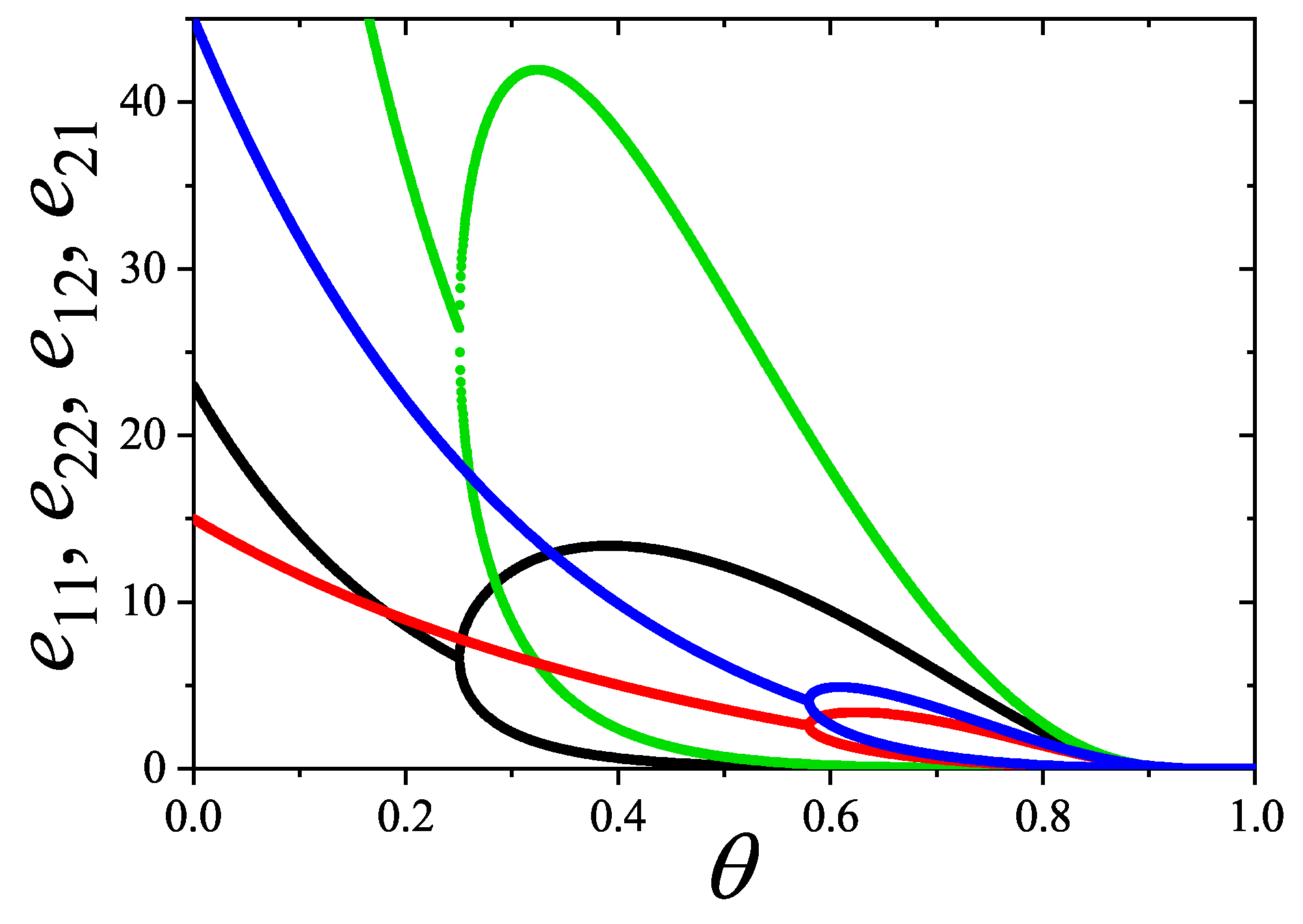
After the transition at , the behavior is as follows: the decreasing branch of indicates stronger alignment and denser packing along ; the decreasing reflects compact transversal packing; the branch of increases sharply beyond , indicating more dispersed -oriented particles; and reaches a maximum and then decreases slightly as density increases.
Since and for , the -oriented phase is always more aligned and compact than the one.
While all vanish at full coverage, the cumulative exclusion functions , defined in Section 6.3, are highly sensitive to changes around the transitions. They split at and show a discontinuous jump at the high-density transition, consistent with its first-order character.
Figure 66.
Average exclusion per particle spectrum functions for and . Red and black: ; blue and green: . Analytical results from statistics formalism.
Figure 66.
Average exclusion per particle spectrum functions for and . Red and black: ; blue and green: . Analytical results from statistics formalism.
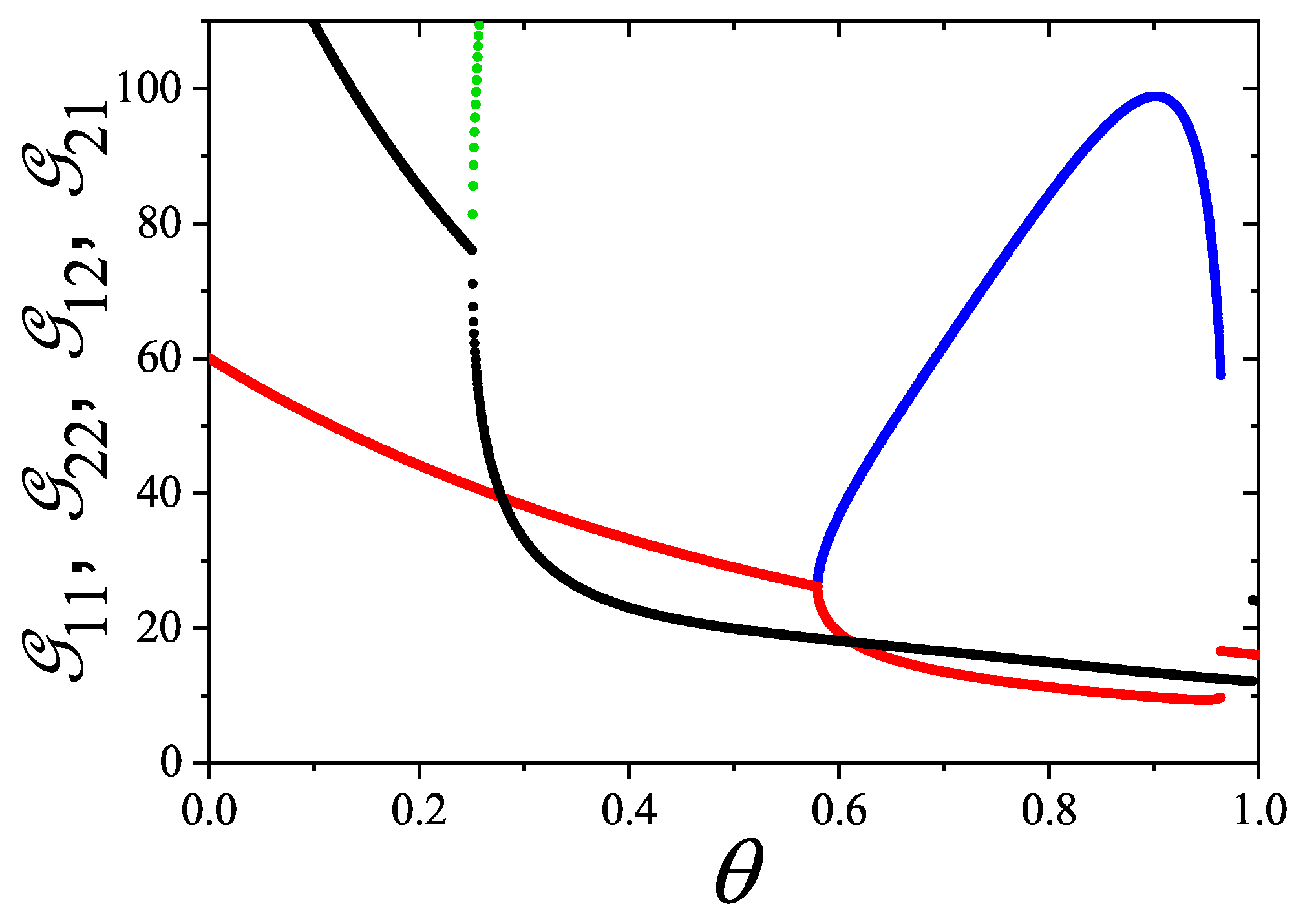
Thus, the functions provide sensitive and valuable analytical tools to trace phase transitions and characterize lattice configurations. Importantly, and can be easily computed in MC simulations.
Regarding the cross-exclusion parameters , they quantify the strength of statistical interaction between - and -oriented k-mers. The leading term shows that controls the exponential decay of available states for particles as particles fill the lattice. Changing variables to and in the isotropic phase, we have
thus
where for . For , , thus no nematic transition is expected.
Qualitatively, in terms of state exclusion statistics, it is the strong depletion of available states for a given orientation, driven by the density of particles in the perpendicular direction, that induces reordering into a nematic phase coexisting with a less dense transverse phase.
Summarizing, the exclusion statistics formulation introduced in Section 6 was applied to address the challenging problem of k-mers on the square lattice due to existence of at least two phase transitions for large . The system was modeled statistically as a mixture of two self-excluding and cross-excluding differently oriented species, or, in equivalent words, as identical particles occupying two different set of states observing self and cross-state exclusion between them because of their topological correlations. The analytical statistics predicts the a continuum isotropic-nematic transition at intermediate coverage only for and, particularly significant, a first-order nematic-isotropic transition at high coverage only for , and less clearly for as well although not as conclusively. The theoretical model reproduces qualitatively and quantitatively well the density dependence of the chemical potential, the lattice coverage and chemical potential at the transitions, it predicts the density branches at the nematic regime as it gives the phase-coexistence line. The formalism provides an accurate approximation for the whole Helmholtz free energy and entropy surfaces in terms of the state occupation numbers, and , of horizontal and vertical k-mers, from which the equilibrium paths are obtained by minimization at fixed average lattice occupation n. The low and high density branches of the adsorption isotherms are accurately reproduced compared to MC simulations. A unified framework was developed by introducing proper thermodynamic averaged state exclusion functions and by expressing them in terms of the k-mers chemical potential and density in order to determine the fundamental statistical correlation parameters from their boundary properties.
8. Monte Carlo Simulation Method Applied to the Problem of Adsorption with Multisite Occupancy
In the following sections, we present different computational algorithms of interest for the study of adsorption problems involving multiple-site occupancy. Most of these algorithms have been used throughout the present work.
8.1. Metropolis MC Algorithms for Adsorption of Interacting k-Mers
8.1.1. Grand Canonical Ensemble
In order to simulate the adsorption/desorption process of k-mers in the grand canonical ensemble, we use a generalized MC algorithm based on the Metropolis scheme of transition probabilities [173]. The method starts with a system of M sites (and connectivity ) at temperature T and pressure P (or chemical potential ). The simulation process is a repetition of the following elementary steps (MCS):
- i)
- set the value of the chemical potential and the temperature T;
- ii)
- choose randomly a linear k-uple of nearest-neighbor sites.
- iii)
- if the k sites selected in are empty, an attempt is made to deposit a rod with probability ; if the k sites selected in are occupied by units belonging to the same k-mer, an attempt is made to desorb this k-mer with probability and otherwise, the attempt is rejected. Here, and represent the probabilities of transition from a state with N particles to a new state with or particles, respectively. Following the Metropolis scheme [174], these probabilities are given by , where is the difference between the Hamiltonians of the final and initial states.
- iv)
- repeat steps M times.
The first MCS of each run are discarded to allow for equilibrium and the next m MCS are used to compute averages. In the low-temperature regime, where ordered phases are expected to develop, displacement (diffusional relaxation) of adparticles to nearest-neighbor positions, by either jumps along the k-mer axis or reptation by rotation around the k-mer end, must be allowed in order to reach equilibrium in a reasonable time.
8.1.2. Canonical Ensemble
In the canonical ensemble, the thermodynamic equilibrium is reached by following Kawasaki’s dynamics [173], generalized to deal with polyatomic molecules. The algorithm to carry out an elementary Monte Carlo step (MCS), is the following:
Given a square lattice of M equivalent adsorption sites:
- i)
- set the value of the temperature T;
- ii)
- set the value of the coverage, , by adsorbing linear molecules onto the lattice, each molecule occupying k adsorption sites;
- iii)
- a k-mer and a linear k-uple of empty sites are randomly selected, and their positions are established. Then, an attempt is made to interchange its occupancy state with probability given by the Metropolis rule [174]:where is the difference between the Hamiltonians of the final and initial states;
- iv)
- a k-mer is randomly selected. Then, a displacement to nearest-neighbor positions is attempted (following the Metropolis scheme), by either jumps along the k-mer axis or reptation by rotation around a unity of the k-mer. This procedure (diffusional relaxation) must be allowed in order to reach equilibrium in a reasonable time; and
- v)
- repeat steps iii)-iv) M times.
As in the case of grand canonical MC simulations presented in Section 8.1.1, the equilibrium state was reached after discarding MCS, and the averages were taken over the next m MCS.
8.2. Parallel Tempering MC Algorithm for Adsorption of Interacting k-Mers
To simulate k-mers of increasing length, the standard grand canonical Monte Carlo (MC) algorithm (Section 8.1.1) typically suffers from slow dynamics, particularly at medium to high coverage. This limitation necessitates the use of alternative algorithms. One such method is the hyper-parallel tempering Monte Carlo (HPTMC) [175] algorithm. The HPTMC method consists in generating a compound system of R non-interacting replicas of the system under study. Each replica is associated with a gas pressure , taken from a set of properly selected pressures [176]. To determine the number of sampled pressures we used an acceptance ratio of for the swapping move for each pair of replicas. Once the values of the gas pressure or the chemical potential are established, the simulation process consist in two major subroutines: replica-update and replica-exchange.
Replica-update.
The adsorption-desorption procedure is as follows: (i) One out of R replicas is randomly selected; (ii) a linear k-uple of nearest-neighbor sites is selected. Then, if the k sites are empty, an attempt is made to deposit a rod with probability ; if the k sites are occupied by units belonging to the same k-mer, an attempt is made to desorb this k-mer with probability and otherwise, the attempt is rejected. As in previous section, .
Replica-exchange.
Exchange of two configurations and , corresponding to the i-th and j-th replicas, respectively, is tried and accepted with probability, , where in a nonthermal grand canonical ensemble is given by,
8.3. Parallel Tempering MC Algorithm for Adsorption of Binary Mixtures of Interacting Species of Polyatomics
The above algorithms, in particular HPTMC, can be applied to the case of mixtures of two species. In order to simulate the adsorption of binary mixtures of k-mers and l-mers we consider a substrate consisting in a regular lattice with connectivity c. The HPTMC method consists in generating a compound system of R non-interacting replicas of the system under study. Each replica is associated with a gas pressure , taken from a set of properly selected pressures [176]. To determine the number of sampled pressures we used an acceptance ratio of for the swapping move for each pair of replicas. Once the values of the gas mixture pressure and molar fractions are set, the chemical potential of each species is obtained an ideal gas mixture, i.e, , where is the standard chemical potential at temperature T and .
Under these considerations, the simulation process consist in two major subroutines: replica-update and replica-exchange.
Replica-update.
The adsorption-desorption procedure is as follows: (i) One out of R replicas is randomly selected; (ii) the species x is selected with equal probability from the two species, k and l; (iii) a linear x-uple of nearest-neighbor sites is selected. Then, if the x sites are empty, an attempt is made to deposit a rod with probability ; if the x sites are occupied by units belonging to the same x-mer, an attempt is made to desorb this x-mer with probability and otherwise, the attempt is rejected.
Replica-exchange.
Exchange of two configurations and , corresponding to the i-th and j-th replicas, respectively, is tried and accepted with probability, , where in a nonthermal grand canonical ensemble is given by,
The complete simulation procedure is the following: (1) replica-update, (2) replica-exchange, and (3) repeat from step (a) times. This is the elementary step in the simulation process or Monte Carlo step (MCs). Typically, the equilibrium state is reached after discarding the first MCs. Then, the next m MCs are used to compute averages.
For each value of pressure , the corresponding surface coverages are determinate by simple averages,
where represents the state of the replica j-th at the Monte Carlo time t.
8.4. Improving the Update Algorithm Through the Use of Lists of Full and Empty k-Uples
By using lists of full and empty k-uples it is possible to improve the performance of previous algorithms. The process of updating (replica-update) involves the random selection of a linear k-uple in the system. This k-uple may turn out to be occupied (by exactly one k-mer or rod), it may be completely empty, or it may have a partial occupation. In the last case the current update process must be rejected. It is possible to perform this random selection in a rejection-free manner using both full and empty k-uples lists. The cost of managing and using the lists is negligible compared to the advantage of avoiding rejection caused by the selection of partially occupied k-uples.
In the case of HPTMC, the procedure is as follows: (i) one out of R replicas is randomly selected; (ii) an element from the compound list of full and empty k-uplas, corresponding to the replica selected in (i), is randomly selected. This element is precisely an empty k-upla or a k-upla occupied by a k-mer. If the k-uple is empty, an attempt is made to deposit a rod with probability ; if the k-uple is occupied, an attempt is made to desorb this k-mer with probability . Finally, if any of the changes have been accepted, the lists of k-uples are updated accordingly.
8.5. Non-Local Update Kundu’s Algorithm for Adsorption of Non-Interacting Large k-Mers (Only Excluded Volume Interaction)
Simulations of k-mers lattice gases were carried out in the Grand Canonical Ensemble through an efficient algorithm introduced by Kundu et al. [101,111,112] to overcome the sampling slowdown at very high density due to the jamming effects. The temperature, chemical potential and system’s size are held fixed and the number of particles on the lattice is allowed to fluctuate through non-local changes, i.e, insertion and deletion of many k-mers at a time (in contrast to the standard Metropolis rule used in previous algorithms).
For a given configuration of k-mers on the square lattice, one MCS is fulfilled by removing all the horizontal k-mers and keeping the vertical ones. This process is shown in Figure 67a,b. Thus, if the system is observed in the horizontal direction, it consists of segments of empty sites of different lengths, separated from each other by vertical k-mers (see for example row j in Figure 67b). The probabilities of having horizontal segments of unoccupied sites can be exactly calculated and stored for all the possible segment sizes (this is essentially a 1D problem). All the horizontal segments are then reoccupied by k-mers and empty sites with the probabilities accordingly determined (see Figure 68). Finally, all these steps are repeated in the vertical direction.
Figure 67 shows the process of removal of horizontal (red) k-mers, and the identification of three segments in a row. Figure 68 shows the process of occupation of a segment. The algorithm can be easily generalized to other geometries and dimensions. The detailed discussion of the algorithm can be found in the original work Refs. [101,111,112]. The algorithm has proved to be ergodic, it satisfies the Detailed Balance Principle and equilibrium is reached after typically MCSs.
8.6. Thermodynamic Integration Method in Canonical Ensemble: Artificial Hamiltonian Method
The advantages of using Monte Carlo simulation to calculate thermal averages of thermodynamic observables are well known [177]. The estimation of certain quantities such as total energy, energy fluctuations, correlation functions, etc., is rather straightforward from averaging over a large enough number of instantaneous configurations (states) of a thermodynamic system. However, free energy and entropy, in general, cannot be directly computed. In order to calculate free energy and entropy, various methods have been developed. Namely, thermodynamic integration method (TIM) [74,75,177,178,179,180], Ma’s method of coincidence counting of states along the trajectory in phase space [181], “stochastic models" method of Alexandrowicz [182], “local states" method of Meirovitch [183], “multistage sampling" and “umbrella sampling" of Valleau et al. [184,185,186,187], method of Salsburg [188], method of Yip et al. [189] (which is an optimized combination of coupling parameter and adiabatic switching formalisms), etc.
Among the methods mentioned in the last paragraph, the TIM is one of the most widely used and practically applicable. In the following, we briefly describe this method.
Given a lattice-gas of N interacting particles on a regular lattice with M sites at temperature T, from the basic relationship
it follows
where U is the mean total energy of the system.
is readily calculated if (reference state) is known, given that the integral in the second term can be accurately estimated by MC simulation. In practice, the calculation of S in a reference state can be rigorously accomplished by analytical methods only in a very few cases. Although the entropy of some particular states is trivially known (for example ), this is often computationally inconvenient since it would require the simulation of a thermodynamic open system to get the entropy of a state at finite density. Alternatively, integration can be carried out through a thermodynamic path of a closed (mechanically isolated) system along a constant density path, if a proper reference state is defined for which can be directly computed.
In the case monomers (), the determination of the entropy in the reference state is trivial. In fact, for a monoatomic lattice-gas
The last equation holds for any finite value of the lateral interactions between the ad-particles.
Since cannot be exactly calculated for k-mer adsorption () by analytical means, in the following we present a general numerical methodology to obtain the entropy of generalized lattice-gas in a reference state.
If an artificial lattice-gas is defined from the system of interest (henceforth referred to as the original system) such that it fulfills the condition,
Then, the integral in Equation (382) can be separated into two terms. Thus,
where and U are the mean total energy of the artificial and original system, respectively (both integrals can be evaluated by MC in the canonical ensemble). The general definition of the artificial reference system follows.
Let us assume the original system to be a discrete system of N particles on M sites with Hamiltonian ; where finite , is the potential energy in the configuration among the set of accessible configurations . The original system can only have access to those configurations within ; the total amount of configurations in is (in a lattice gas of N monomers with single-site occupancy of M sites, ).
The Hamiltonian for the artificial system, , follows from:
Definition 1: , is defined as finite , where and have analogous meanings to those given above for U and , respectively. The equalities ensure that the set of accessible configurations for the original system and the artificial system are equal (although , the energy of the configurations in the artificial system may be, in general, different from the ones in the original system).
Definition 2: The potential energy of the accessible configurations () for the artificial system take the following values
Definition 2 means that a given configuration (the th) is selected arbitrarily from and defined as the non-degenerate ground state of the artificial lattice-gas; hence . In practice, the configuration can be easily defined.
An example for adsorbed dimers follows in order to make this point clear. Let us consider adsorbed dimers on an homogeneous square lattice with and interaction between NN dimer’s heads as shown in Figure 69 (original system). For this system there is no rigorous expression of for in the thermodynamic limit (, constant).
To build up an artificial system fulfilling the definitions 1 and 2, we follow the steps:
The number of particles, size and geometry of the lattice is kept as in the original system.
The interaction energy between NN units is set to zero.
An adsorption energy is introduced for the lattice sites (representing, for each site, the interaction between the lattice and the unit of the dimer adsorbed on it in the artificial system), in such a way that two types of sites are defined, strong and weak, with energies and , respectively, being . For N adsorbed dimers we choose strong sites conveniently on the lattice. For instance, in Figure 70a a possible distribution of strong and weak sites is depicted, where circles and squares are sites of energy and , respectively.
It is assumed that dimers in a particular direction are energetically favored. This is formally handled by introducing a virtual external field such that the interaction energy between the dimers and the field is if the dimer is vertically aligned and otherwise (this choice is obviously arbitrary). Care must be taken if periodic boundary conditions are applied to ensure that the state of minimum energy is unique. Then, the Hamiltonian of the artificial system for this example is given by
where if the site is strong and if the site is weak.
Thus, the ground state of the artificial system is the one shown in Figure 70(b), which is non-degenerate, giving .
The calculation of through Equation (386) is straightforward and computationally simple, since the temperature dependence of and is evaluated at constant coverage for various values of T following the standard procedure of MC simulation in the canonical ensemble (see Section 8.1.2) (based on the Metropolis scheme [174]). Then, and are obtained as simple averages, spline-fitted and numerically integrated. It should be mentioned that is calculated by using the hamiltonian of Equation (388) and is calculated by using the original hamiltonian. Two typical curves of versus u are shown in Figure 71, for attractive and repulsive dimers on a square lattice.
The strategy described above is applicable to a wide class of lattice-gas systems.
9. Conclusions and Future Perspectives
This review has systematically explored the thermodynamic behavior and statistical mechanics of adsorbed rigid rods (or k-mers) on regular lattices, focusing on equilibrium properties as a function of density, temperature, and particle size. Through a sequence of progressively refined approaches—ranging from exact results in one dimension to numerical simulations and mean-field approximations in higher dimensions, and culminating in the analytical development of Multiple Exclusion (ME) statistics—the article provides a broad and coherent framework for understanding collective adsorption phenomena governed by excluded volume effects.
In Section 2, the review focused on one-dimensional (1D) systems, which offer the unique opportunity of exact solvability. The classic lattice versions of hard rod systems are revisited, emphasizing their exact entropy, equation of state, and chemical potential. These models serve not only as rigorous benchmarks but also as reference systems to test approximate theories. Thus single-species and mixtures on the lattice can be rigorously treated and phenomena such as reversal-adsorption in binary mixtures can be well characterized and understood in the light of the model system. The treatment of k-mers in the multilayer regime bears an elucidating relation with analogous experimental realizations such as adsorption of linear molecules (alkanes, alkenes) on quasi-regular surfaces of carbon nanotubes leading to demonstrate that molecular the size/shape entropic contribution to free energy cannot be oversimplified in interpreting adsorption isotherms to determine the specific surface of the adsorbent.
The inclusion of interacting k-mers through lateral attractions or repulsions further enriches the 1D landscape, allowing for a better understanding of the features of the coverage dependence of entropy. Notably, the exact solutions for lattice k-mers lay the groundwork for understanding the role of orientational and configurational constraints in low-dimensional systems.
The 1D treatment sets the basis for extending the understanding to higher dimensions by introducing coarse-grained approaches that effectively capture key thermodynamic quantities. Here, the notion of excluded volume per particle is generalized, leading to approximate expressions for entropy and pressure that remain remarkably accurate across a broad range of densities. A number of approximations were reviewed, ranging from the configurational dimensional ansatz to extend the 1D analytical forms to higher dimensions through the EA approximation, the conceptualization of the challenging problem of the structured particles lattice gas as one isomorphic to fractional exclusion statistics in quantum systems with independent states through FSTA, up to the introduction of the most elaborate theoretical approach, named Multiple Exclusion Statistics, embodying the complexity emerging from spatial correlations between particle states into a set of simple self-exclusion and cross-exclusion correlation parameters that can be consistently determined within the theory from limiting configurational conditions of the system. .
The article then progresses to address more intricate systems in higher dimensions, where exact solutions are generally not accessible. Here, mean-field approximations and phenomenological entropy-based models are employed to describe the emergence of phase transitions, particularly the isotropic-to-nematic transition observed for elongated particles. These transitions are governed not only by steric constraints but also by emergent orientational ordering, which is absent in 1D. The entropy per site as a function of coverage reveals non-trivial behavior, including entropy-driven phase separations and coexistence regions, which can be tracked even in approximate analytical formulations.
Section 4 presents a series of heuristic and mean-field-like methods aimed at incorporating orientational degrees of freedom and spatial correlations in 2D and 3D lattices. The simple Bragg-Williams-type approximations provide qualitative insights into isotropic-nematic transitions and the role of k-mer length. Improved approaches, such as those based on lattice free volume estimates or effective excluded area models like the Quasi-Chemical approach, offer better agreement with simulation data, particularly. However, these approximations often neglect inter-particle correlations and fail to describe critical behavior accurately.
The review takes a major conceptual leap in Section 5 and Section 6, where the statistical description of the system is reframed through the lens of generalized exclusion statistics, particularly in the form of Multiple Exclusion (ME) statistics. This approach introduces the idea of state-counting based on effective exclusion rules that go beyond simple geometric packing. By systematically encoding how a particle’s presence affects the availability of nearby states, the ME formalism captures both entropic interactions and emergent correlations. This represents a profound shift from traditional lattice gas models toward a more abstract and generalizable statistical mechanics framework.
One of the most significant achievements of this formalism is the derivation of spectral exclusion functions, which encode the exclusion parameters between particle states. These functions allow for the construction of thermodynamic quantities—such as the chemical potential and entropy from the statistical exclusion rules, circumventing the need for explicit partition functions. Furthermore, the ability to reproduce not only exact 1D results but also to approximate higher-dimensional behavior with improved accuracy underscores the power of the ME approach.
A key theoretical development discussed is the formalization of ME statistics to include multi-component and geometrically complex particle mixtures. The introduction of state self-exclusion and state cross-exclusion functions and , as generalizations of chemical potential derivatives with respect to partial densities, allows for a thermodynamic characterization of complex exclusion scenarios. These spectral functions encode how the presence of particles of one species affects the availability of configurations for others, thus extending the exclusion principle into a spatially resolved thermodynamic descriptor.
It is also showcased the application of these ideas to realistic systems (Section 7), such as adsorption on heterogeneous surfaces, adsorption of alkanes on carbon nanotubes as a prototype experimental realization to show the simplest multilayer adsorption model generalizing the pioneer work of BET to determine adsorption energy and specific area of adsorbent when probe molecules are not ideally spherical. Furthermore, application to crystal growth from aqueous solutions in presence of structured impurities were exhibited as applications were the impurity size and shape must be properly accounted for in the thermodynamic potentials in order to understand the growth rate dependence on impurity concentration.
The application examples concluded with an in-depth analysis of the long-standing k-mer problem on the square lattice, approached through the advanced framework of Multiple Exclusion Statistics theory. This problem, which still presents several open questions, such as the lack of a unified theoretical explanation for the emergence of a nematic transition at the critical length , and the nature of the high-density transition back to an isotropic phase near saturation, was revisited from the alternative and more comprehensive perspective provided by the ME formalism. By modeling the system as a mixture of two species of particles with distinct orientations, the free energy and entropy surfaces were analytically approximated across the full range of relative occupations along lattice directions. This approach enabled a detailed characterization of density branches, critical points, transition orders, and exclusion spectrum functions, offering new insights into the entropy–density relationship. The analysis reveals that is the minimal rod length required to undergo a nematic transition, while , although close, does not satisfy the necessary conditions and remains in an isotropic phase even at high coverage.
Furthermore, the review explores the novel outcomes of ME statistics such as the potential of extracting exclusion spectral functions from experimental data, inverting thermodynamic observables to infer structural information. This opens the possibility of using adsorption isotherms and fluctuations spectra not just as phenomenological descriptors, but as quantitative probes of configurational entropy and microstate topology. Remarkably, the ME statistics theoretical framework provides a bridge between observable thermodynamic quantities (e.g., chemical potential versus density curves) and latent spatial correlations or ordering tendencies that are otherwise hidden. This fact opens new experimental possibilities: exclusion spectra may eventually be inferred from measurements of adsorption isotherms or compressibility, providing insight into microscopic ordering without relying on direct imaging.
Ultimately, the ME formalism proves to be a unifying language capable of handling complex interactions and geometry-induced constraints. It not only serves as a powerful lens for interpreting equilibrium properties of complex particle systems, but also sets the stage for future theoretical and experimental explorations into the geometry and thermodynamics of constrained configuration spaces.
Several open questions and research avenues arise from this unified perspective. First, the extension of ME statistics to non-lattice systems, including continuous 2D and 3D domains with quenched disorder or curved geometries, remains largely unexplored.
Its generality and compatibility with empirical data make it not only a theoretical construct but also a bridge toward experimentally accessible quantities. From a computational standpoint, there is room for developing inverse statistical mechanical methods that reconstruct exclusion spectral functions directly from experimental data or Monte Carlo simulations. This would establish a concrete protocol for extracting statistical fingerprints from real systems, with applications in surface science, porous media, and biological adsorption.
Secondly, dynamical aspects such as adsorption/desorption kinetics, diffusion on fluctuating energy landscapes, or driven systems under external fields, are fertile grounds for applying and testing the ME framework beyond equilibrium.
Looking ahead, the ME framework is poised to play a central role in the statistical mechanics of systems with constrained configurations, such as crowding in biological environments, adsorption in porous media, or active matter with limited motility space.
Finally, there is potential to link the ME statistics approach with field-theoretic and renormalization group methods, particularly in systems where critical behavior or universality classes may be modified by spatial exclusion. The interplay between exclusion-driven entropy and geometric frustration also presents an intriguing challenge, especially in contexts where topology and boundary effects play a dominant role.
A whole Section 8 was devoted to review the Monte Carlo techniques from the early Metropolis state sampling to the new highly efficient non-local configuration update to overcome the sampling slowdown to reach equilibrium in lattice gases with state exclusion, particularly at high density. Furthermore, the artificial-Hamiltonian technique was revisited as powerful tool to calculate entropy at arbitrary density from elementary thermodynamic relations taking advantage of efficient numerical sampling of equilibrium configurations.
Monte Carlo (MC) simulations serve as an essential tool to validate approximate analytical methods for single components and mixtures as well as exploring the influence of the lattice geometry on the thermodynamic potentials. MC studies have uncovered rich phase behavior, including continuous and discontinuous isotropic-nematic transitions, as well as layering and jamming effects near full coverage. These results have helped to clarify the limitations of earlier mean-field approximations and motivated the development of more refined theories. Importantly, the numerical data have also inspired empirical functional forms for entropy and chemical potential, which have been instrumental in bridging the gap between simulations and analytical descriptions. The multiple exclusion problem opens new questions concerning potential simulation techniques in systems with strong state correlations and geometrical constrains exploiting the topological properties of the configuration space and graph theory.
In summary, this article accomplishes several goals: It consolidates a wide range of exact, approximate, and numerical results across spatial dimensions and k-mer lengths, it clarifies the domain of validity and limitations of various theoretical approaches, it reviews the recently presented Multiple Exclusion Statistics (ME) as a promising analytical tool that reconciles geometric exclusion under topological constrains and correlations with thermodynamic consistency and it sets new perspectives for the application and testing of this newest analytical tool to a broader scenario of systems where spatial correlations of particle states dominate.
The synthesis of exact models, approximate theories, numerical validation, and generalized statistics presented in this review thus offers a comprehensive and forward-looking perspective on k-mer adsorption and excluded volume systems, with broader implications across condensed matter, materials science, and statistical physics.
Author Contributions
J.J. Riccardo: Investigation, Formal analysis, Software, Methodology. P.M. Pasinetti: Investigation, Formal analysis, Software, Methodology. J.L. Riccardo: Conceptualization, Supervision, Methodology, Writing – original draft, Writing – review & editing. A.J. Ramirez-Pastor: Conceptualization, Supervision, Methodology, Writing – original draft, Writing – review & editing, Project administration, Funding acquisition.
Data Availability Statement
Dataset available on request from the authors
Acknowledgments
This work was supported in part by CONICET (Argentina) under Project No. PIP 11220220100238CO and Universidad Nacional de San Luis (Argentina) under Project 03-1920. The numerical work were done using the BACO parallel cluster located at Instituto de Física Aplicada, Universidad Nacional de San Luis - CONICET, San Luis, Argentina.
Conflicts of Interest
The authors declare no conflicts of interest.
References
- Onsager, L. The effects of shape on the interaction of colloidal particles. Ann. N. Y. Acad. Sci. 1949, 51, 627–659. [CrossRef]
- Kasteleyn, P. The statistics of dimers on a lattice I. The number of dimer arrangements on a quadratic lattice. Physica 1961, 27, 1209–1225. [CrossRef]
- Baxter, R.J. Hard hexagons: exact solution. J. Phys. A: Math. Gen. 1980, 13, L61–L70. https://iopscience.iop.org/article/10.1088/0305-4470/13/3/007.
- Frenkel, D.; Eppenga, R. Evidence for algebraic orientational order in a two-dimensional hard-core nematic. Phys. Rev. A 1985, 31, 1776–1787. [CrossRef]
- Khandkar, D.; Barma, M. Orientational correlations and the effect of spatial gradients in the equilibrium steady state of hard rods in two dimensions: A study using deposition-evaporation kinetics. Phys. Rev. E 2005, 72, 051717. https://journals.aps.org/pre/abstract/10.1103/PhysRevE.72.051717.
- Flory, P.J. Thermodynamics of High Polymer Solutions. J. Chem. Phys. 1942, 10, 51–61. [CrossRef]
- Huggins, M.L. Some properties of solutions of long-chain compounds. J. Chem. Phys. 1942, 46, 151–158. https://pubs.acs.org/doi/abs/10.1021/j150415a018.
- Des Cloizeaux, J.; Jannink, G. Polymers in Solution. Their Modelling and Structure; Clarendon Press: Oxford, UK, 1990. [CrossRef]
- DiMarzio, E.A. Statistics of Orientation Effects in Linear Polymer Molecules. J. Chem. Phys. 1961, 35, 658–669. [CrossRef]
- Guggenheim, E.A. Statistical Thermodynamics of Mixtures with Zero Energies of Mixing. Proc. R. Soc. London 1944, A183, 203–212. [CrossRef]
- Romá, F.; Riccardo, J.L.; Ramirez-Pastor, A.J. Semiempirical Model for Adsorption of Polyatomics. Langmuir 2006, 22, 3192–3197. [CrossRef]
- Riccardo, J.L.; Romá, F.; Ramirez-Pastor, A.J. Fractional Statistical Theory of Adsorption of Polyatomics. Phys. Rev. Lett. 2004, 93, 186101. [CrossRef]
- Riccardo, J.L.; Romá, F.; Ramirez-Pastor, A.J. Generalized statistical description of adsorption of polyatomics. Applied Surf. Sci. 2005, 252 505–511. [CrossRef]
- Haldane, F.D.M. “Fractional statistics" in arbitrary dimensions: A generalization of the Pauli principle Phys. Rev. Lett. 1991, 67, 937–940. [CrossRef]
- Wu, Y.S. Statistical distribution for generalized ideal gas of fractional-statistics particles. Phys. Rev. Lett. 1994, 73, 922–925. [CrossRef]
- Riccardo, J.L.; Romá, F.; Ramirez-Pastor, A.J. Adsorption of polyatomics: theoretical approaches in model systems and applications. Int. J. Mod. Phys. B 2006, 20, 4709–4778. [CrossRef]
- Riccardo, J.J.; Riccardo, J.L.; Ramirez-Pastor, A.J.; Pasinetti, P.M. Multiple Exclusion Statistics. Phys. Rev. Lett. 2019, 123, 020602. [CrossRef]
- Riccardo, J.J.; Pasinetti, P.M.; Ramirez-Pastor, A.J.; Riccardo, J.L. Exclusion statistics for structured particles on topologically correlated states. I. Single species lattice gases. Phys. Rev. E 2025, 111, 014122. [CrossRef]
- Riccardo, J.J.; Pasinetti, P.M.; Ramirez-Pastor, A.J.; Riccardo, J.L. Exclusion statistics for structured particles on topologically correlated states. II. Multicomponent lattice gases. Phys. Rev. E 2025, 111, 014123. [CrossRef]
- Ramirez-Pastor, A. J.; Eggarter, T. P.; Pereyra, V.; Riccardo, J. L. Statistical thermodynamics and transport of linear adsorbates, Phys. Rev. B 1999, 59, 11027-11036. [CrossRef]
- Kasteleyn, P. Dimer Statistics and Phase Transitions. J. Math. Phys. 1963, 4, 287–293. [CrossRef]
- Temperley, H N.V.; Fisher, M.E. Dimer problem in statistical mechanics—an exact result. Philos. Mag. 1961, 6, 1061–1063. [CrossRef]
- Fisher, M.E. Statistical mechanics of dimers on a plane lattice. Phys. Rev. 1961, 124, 1664–1672. [CrossRef]
- Phares, A.J.; Wunderlich, F.J.; Grumbine, D.W.; Curley, J.D. The entropy curves for interacting dimers on a square lattice. Phys. Lett. A 1993, 173, 365–368. [CrossRef]
- Phares, A.J.; Wunderlich, F.J. Thermodynamics of dimers on a rectangular L × M × N lattice. J. Math. Phys. 1985, 26, 2491–2499. [CrossRef]
- Phares, A. J.; Wunderlich, F.J. Thermodynamics and Molecular Freedom of Dimers on Plane Triangular Lattices. J. Math. Phys. 1986, 27, 1099–1109. [CrossRef]
- Phares, A.J.; Wunderlich, F.J. Thermodynamics and Molecular Freedom of Dimers on Plane Honeycomb and Kagomé Lattices. Il Nuovo Cimento B 1988, 301, 653–686. [CrossRef]
- W. Rżysko, W.; Patrykiejew, A.; Binder, K. Phase transitions in a two-dimensional lattice gas model of orientable diatomic molecules. Phys. Rev. B 2005, 72, 165416. [CrossRef]
- Wu, F.Y. Dimers on two-dimensional lattices. Int. J. Mod. Phys. B 2006, 20, 5357–5371. [CrossRef]
- Dávila, M.; Romá, F.; Riccardo, J.L.; Ramirez-Pastor, A.J. Quasi-chemical approximation for polyatomics: Statistical thermodynamics of adsorption. Surf. Sci. 2006, 600, 2011–2025. [CrossRef]
- Dávila, M.; Riccardo, J.L.; Ramirez-Pastor, A.J. Fractional statistical theory and use of quasi-chemical approximation for adsorption of interacting k-mers. Surf. Sci. 2009, 603, 683–689. [CrossRef]
- Marczewski, A. W.; Derylo-Marczewska, M.; Jaroniec, M. Energetic heterogeneity and molecular size effects in physical adsorption on solid surfaces. J. Colloid Interface Sci. 1986, 109, 310–324. [CrossRef]
- Nitta, T.; Kuro-Oka, M.; Katayama, T. An adsorption isotherm of multi-site occupancy model for heterogeneous surface. J. Chem. Eng. Jpn. 1984, 17, 45–52. [CrossRef]
- Nitta, T.; Yamaguchi, A. J. A hybrid isotherm equation for mobile molecules adsorbed on heterogeneous surface of random topography. J. Chem. Eng. Jpn. 1992, 25, 420–426. [CrossRef]
- Rudziński, W.; Lajtar, L.; Zaja̧c, J.; Wolfram, E.; Pászli, I. Ideal adsorption from binary liquid mixtures on heterogeneous solid surfaces: Equations for excess isotherms and heats of immersion. J. Colloid Interface Sci. 1983, 96, 339–359. [CrossRef]
- Rudziński, W.; Zaja̧c, J.; Hsu, C. C. Excess isotherms and heats of immersion in monolayer adsorption from binary liquid mixtures on strongly heterogeneous solid surfaces. J. Colloid Interface Sci. 1985, 103, 528–541. [CrossRef]
- Rudziński, W.; Everett, D.H. Adsorption of gases on heterogeneous surfaces; Academic Press, London, UK, 1992. [CrossRef]
- Iijima, S. Helical microtubules of graphitic carbon. Nature 1991, 345, 56–58. [CrossRef]
- Iijima, S.; Ichihaschi, T. Single-shell carbon nanotubes of 1-nm diameter. Nature 1993, 363, 603–605. [CrossRef]
- Bethune, D.S.; Kiang, C.H.; de Vries, M.S.; Gorman, G.; Savoy, R.; Vazquez, J.; Beyers, R. Cobalt-catalysed growth of carbon nanotubes with single-atomic-layer walls. Nature 1993, 363, 605–607. [CrossRef]
- Ajayan, P.M.; Iijima, S. Capillarity-Induced Filling of Carbon Nanotubes. Nature 1993, 361, 333–334. [CrossRef]
- Deurbergue, A.; Oberlin, A. TEM study of some recent high modulus pan-based carbon fibers. Carbon 1992, 30, 981–987. [CrossRef]
- Martin, J.C.; Coulomb, J.P.; Grillet, V.; Kahn, R. Measure of the Translational Mobility Dt of Methane Molecules Sorbed in the One-Dimensional Micropore Network of the AlPO4-5 Zeolite. In Fundamentals of Adsorption; Le Van, M.D., Ed.; Kluwer Academic Publishers: Boston, USA, 1996; pp. 587–594.
- Rittner, F.; Boddenberg, B.; Bojan, M. J.; Steele, W.A. Adsorption of Nitrogen on Rutile (110): Monte Carlo Computer Simulations. Langmuir 1999, 15, 1456–1462. [CrossRef]
- Maddox, M.W.; Ulberg, D.; Gubbins, K.E. Molecular simulation of simple fluids and water in porous carbons. Fluid Phase Equilibria 1995, 104, 145–158. [CrossRef]
- Maddox, M.W.; Gubbins, K.E. Molecular Simulation of Pure Fluid and Binary Mixture Adsorption in Buckytubes and MCM-41. In Fundamentals of Adsorption; Le Van, M.D., Ed.; Kluwer Academic Publishers: Boston, USA, 1996; pp. 563–570.
- Stan, G.; Cole, M. W. Low coverage adsorption in cylindrical pores. Surf. Sci. 1998, 395, 280–291. [CrossRef]
- Stan, G.; Crespi, V.H.; Cole, M.W.; Boninsegni, M. J. Interstitial He and Ne in Nanotube Bundles. J. Low Temp. Phys. 1998, 113, 447–452. [CrossRef]
- Maltz, A.; Mola, E. E. Pair site occupation probability for one-dimensional array of dumbbells. J. Math. Phys. 1981, 22, 1746–1748. [CrossRef]
- Hill, T. L. An Introduction to Statistical Thermodynamics; Addison-Wesley: Reading, USA, 1960.
- Khettar, A.; Jalili, S.E.; Dunne, L.J.; Manos, G.; Du, Z. Monte-Carlo simulation and mean-field theory interpretation of adsorption preference reversal in isotherms of alkane binary mixtures in zeolites at elevated pressures. Chem. Phys. Lett. 2002, 362, 414–418. [CrossRef]
- Dunne, L.J.; Manos, G.; Du, Z. Exact statistical mechanical one-dimensional lattice model of alkane binary mixture adsorption in zeolites and comparision with Monte-Carlo simulations. Chem. Phys. Lett. 2003, 377, 551–556. [CrossRef]
- Clark, A. The Theory of Adsorption and Catalysis; Academic Press: New York, USA, 1970.
- Gregg, S.J.; Sing, K.S.W. Adsorption, Surface Area, and Porosity; Academic Press: New York, USA, 1991.
- Adamson, A.W. Physical Chemistry of Surfaces; John Wiley and Sons: New York, USA, 1990.
- Frenkel, J. Kinetic Theory of Liquids; Dover Reprint: New York, USA 1955.
- Halsey, G.D. Physical Adsorption on Non-Uniform Surfaces. J. Chem. Phys. 1948, 16, 931–937. [CrossRef]
- Hill, T.L. Theory of Physical Adsorption. Adv. Catal. 1952, 4, 211–258. [CrossRef]
- McMillan, W.G.; Teller, E. The Role of Surface Tension in Multilayer Gas Adsorption. J. Chem. Phys. 1951, 19, 25–32. [CrossRef]
- Brunauer, S.; Emmett, P.H.; Teller, E. Adsorption of Gases in Multimolecular Layers. J. Am. Chem. Soc. 1938, 60, 309–319. [CrossRef]
- Pierce, C.; Ewing, B. Areas of Uniform Graphite Surfaces. J. Phys. Chem. 1964, 68, 2562–2568. [CrossRef]
- Aligia, A.A. One-dimensional oxygen ordering in YBa2Cu3O7-δ. Phys. Rev. B 1993, 47, 15308–15311. [CrossRef]
- Kikuchi, R. A Theory of Cooperative Phenomena. Phys. Rev. B 1951, 81, 988–1003. [CrossRef]
- Martin, J.C.; Tosi-Pellenq, N.; Patarin, J.; Coulomb, J.P. Sorption Properties of AlPO4-5 and SAPO-5 Zeolite-like Materials. Langmuir 1998, 14, 1774–1778. [CrossRef]
- Lachet, V.; Boutin, A.; Pellenq, R.M.; Nicholson, D.; Fuchs, A. Molecular Simulation Study of the Structural Rearrangement of Methane Adsorbed in Aluminophosphate AlPO4-5. J. Phys. Chem. 1996, 100, 9006–9013. [CrossRef]
- Maris, T.; Vlugt, T.J.H.; Smit, B. Simulation of Alkane Adsorption in the Aluminophosphate Molecular Sieve AlPO4-5. J. Phys. Chem. B 1998, 102, 7183–7189. [CrossRef]
- Steele, W.A. The Interaction of Gases with Solid Surfaces; Pergamon Press: New York, USA, 1974.
- A. Patrykiejew, A.; Sokolowski, S. Statistical mechanics of adsorption of polyatomic molecules on solid surfaces. Advances in Colloid and Interface Science 1989, 30, 203–334. [CrossRef]
- Zimm, B.H. Application of the Methods of Molecular Distribution to Solutions of Large Molecules. J. Chem. Phys. 1946, 14, 164–179. [CrossRef]
- Isihara, A. Determination of Molecular Shape by Osmotic Measurement. J. Chem. Phys. 1950, 18, 1446–1449. [CrossRef]
- Isihara, A. Theory of Anisotropic Colloidal Solutions. J. Chem. Phys. 1951, 19, 1142–1147. [CrossRef]
- Ramirez-Pastor, A.J.; Pereyra, V.D.; Riccardo, J.L. Statistical Thermodynamics of Linear Adsorbates in Low Dimensions: Application to Adsorption on Heterogeneous Surfaces. Langmuir 1999, 15, 5707–5712. [CrossRef]
- Romá, F.; Ramirez-Pastor, A.J.; Riccardo, J.L. Multisite Occupancy Adsorption: Comparative Study of New Different Analytical Approaches. Langmuir 2003, 19, 6770–6777. [CrossRef]
- Romá, F.; Ramirez-Pastor, A.J.; Riccardo, J.L. Configurational Entropy in k-mer Adsorption. Langmuir 2000, 16, 9406–9409. [CrossRef]
- Romá, F.; Ramirez-Pastor, A.J.; Riccardo, J.L. Configurational entropy for adsorbed linear species (k-mers). J. Chem. Phys. 2001, 114, 10932–10937. [CrossRef]
- Gujrati, P.D.; Chhajer, M. New statistical mechanical treatment of systems near surfaces. I. Theory and principles. J. Chem. Phys. 1997, 106, 5599–5614. [CrossRef]
- Peterson, H.T.; Martire, D.E.; Cotter, M.A. Lattice model for a binary mixture of hard rods of different lengths. Application to solute induced nematic→isotropic transitions. J. Chem. Phys. 1974, 61, 3547–3555. [CrossRef]
- Dávila, M.; Riccardo, J.L.; Ramirez-Pastor, A.J. Exact statistical thermodynamics of alkane binary mixtures in zeolites: New interpretation of the adsorption preference reversal phenomenon from multisite-occupancy theory. Chem. Phys. Lett. 2009, 477, 402–405. [CrossRef]
- Riccardo, J.L.; Ramirez-Pastor, A.J.; Romá, F. Multilayer Adsorption with Multisite Occupancy: An Improved Isotherm for Surface Characterization. Langmuir 2002, 18, 2130–2134. [CrossRef]
- Patrykiejew, A.; Sokolowski, S.; Binder, K. Phase transitions in adsorbed layers formed on crystals of square and rectangular surface lattice. Surf. Sci. Rep. 2000, 37, 207–344. [CrossRef]
- Plischke, M.; Bergersen, B. Equilibrium Statistical Physics; Prentice Hall: New Jersey, USA, 1989. [CrossRef]
- Goldenfeld, N. Lectures on phase transitions and the renormalization group; CRC Press: Boca Raton, FL, USA, 2018. [CrossRef]
- Yeomans, J.M. Statistical Mechanics of Phase Transitions; Clarendon Press: Oxford, UK, 1992.
- Ising, E. Beitrag zur Theorie des Ferromagnetismus. Z. Physik 1925, 31, 253–258. [CrossRef]
- Domb, C. Series Expansions for Lattice Models. In Phase transitions and critical phenomena, vol. 3; Domb, C.; Green, M.S., Eds.; Academic Press: London, UK, 1974; pp. 1–95.
- Fisher, M.E. The theory of equilibrium critical phenomena. Rep. Prog. Phys. 1967, 30, 615–730. https://iopscience.iop.org/article/10.1088/0034-4885/30/2/306.
- Onsager, L. Crystal Statistics. I. A Two-Dimensional Model with an Order-Disorder Transition. Phys. Rev. 1944, 65, 117–149. [CrossRef]
- Bethe, H.A. Statistical theory of superlattices. Proc. R. Soc. London 1935, A150, 552–575. [CrossRef]
- Quiroga, E.; Ramirez-Pastor, A.J. Statistical thermodynamics of molecules with multiple adsorption states: Application to protein adsorption. Chem. Phys. Lett. 2013, 556, 330–335. [CrossRef]
- Dhar, D.; Rajesh, R. Entropy of fully packed hard rigid rods on d-dimensional hypercubic lattices. Phys. Rev. E 2021, 103, 042130. [CrossRef]
- Rodrigues, L.R.; Stilck, J.F.; Dantas, W.G. Entropy of rigid k-mers on a square lattice. Phys. Rev. E 2023, 107, 014115. [CrossRef]
- Lambert, J.H. Observationes variae in mathesin puram. Acta Helveticae Physico-Mathematico-Anatonico-Botanico-Medica 1758, 3, 128–168.
- Scott, T.C.; Aubert-Frécon, M.; Grotendorst, J. New approach for the electronic energies of the hydrogen molecular ion. Chem. Phys. 2006, 324, 323–338. [CrossRef]
- Scott, T.C.; Lüchow, A.; Bressanini, D.; Morgan, J. D. Nodal surfaces of helium atom eigenfunctions. Phys Rev. A 2007, 75, 060101(R). [CrossRef]
- Farrugi, P.S.; Mann, R.B.; Scott, T.C. N-body gravity and the Schrödinger equation. Class. Quantum Grav. 2007, 24, 4647–4659. https://iopscience.iop.org/article/10.1088/0264-9381/24/18/006.
- Ghosh, A.; Dhar, D. On the orientational ordering of long rods on a lattice. Eur. Phys. Lett. 2007, 78, 20003. https://iopscience.iop.org/article/10.1209/0295-5075/78/20003.
- Matoz-Fernandez, D.A.; Linares, D.H.; Ramirez-Pastor, A.J. Determination of the critical exponents for the isotropic-nematic phase transition in a system of long rods on two-dimensional lattices: Universality of the transition. Eur. Phys. Lett. 2008, 82, 50007. https://iopscience.iop.org/article/10.1209/0295-5075/82/50007.
- Matoz-Fernandez, D.A.; Linares, D.H.; Ramirez-Pastor, A.J. Critical behavior of long straight rigid rods on two-dimensional lattices: Theory and Monte Carlo simulations. J. Chem. Phys. 2008, 128, 214902. [CrossRef]
- Matoz-Fernandez, D.A.; Linares, D.H.; Ramirez-Pastor, A.J. Critical behavior of long linear k-mers on honeycomb lattices. Physica A 2008, 387, 6513–6525. [CrossRef]
- Disertori, M.; Giuliani, A. The Nematic Phase of a System of Long Hard Rods. Commun. Math. Phys. 2013, 323, 143–175. [CrossRef]
- Kundu, J.; Rajesh, R.; Dhar, D.; Stilck, J.F. Nematic-disordered phase transition in systems of long rigid rods on two-dimensional lattices. Phys. Rev. E 2013, 87, 032103. [CrossRef]
- Chatelain, C.; Gendiar, A. Absence of logarithmic divergence of the entanglement entropies at the phase transitions of a 2D classical hard rod model. Eur. Phys. J. B 2020, 93, 134. [CrossRef]
- Kundu, J.; Rajesh, R. Reentrant disordered phase in a system of repulsive rods on a Bethe-like lattice. Phys. Rev. E 2013, 88, 012134. [CrossRef]
- Vogel, E.E.; Saravia, G.; Ramirez-Pastor, A.J. Phase transitions in a system of long rods on two-dimensional lattices by means of information theory. Phys. Rev. E 2017, 96, 062133. [CrossRef]
- Vogel, E.E.; Saravia, G.; Ramirez-Pastor, A.J.; Pasinetti, M. Alternative characterization of the nematic transition in deposition of rods on two-dimensional lattices. Phys. Rev. E 2020, 101, 022104. [CrossRef]
- Shah, A.; Dhar, D.; Rajesh, R. Phase transition from nematic to high-density disordered phase in a system of hard rods on a lattice. Phys. Rev. E 2022, 105, 034103. [CrossRef]
- Pasinetti, P.M.; Ramirez-Pastor, A.J.; Vogel, E.E.; Saravia, G. Entropy-driven phases at high coverage adsorption of straight rigid rods on two-dimensional square lattices. Phys. Rev. E 2021, 104, 054136. [CrossRef]
- Dhar, D.; Rajesh, R.; Stilck, J.F. Hard rigid rods on a Bethe-like lattice. Phys. Rev. E 2011, 84, 011140. [CrossRef]
- Centres, P.M.; Ramirez-Pastor, A.J. Configurational entropy of adsorbed rigid rods: Theory and Monte Carlo simulations. Physica A 2009, 388, 2001–2019. [CrossRef]
- De La Cruz Feliz, N.M.; De La Cruz Félix, N.; Quiroga, E.; Riccardo, J.J.; Riccardo, J.L.; Ramirez Pastor, A.J. Fractional statistics description applied to adsorption of trimers on triangular lattices, in preparation.
- Kundu, J.; Rajesh, R. Phase transitions in a system of hard rectangles on the square lattice. Phys. Rev. E 2014, 89, 052124. [CrossRef]
- Kundu, J.; Rajesh, R.; Dhar, D.; Stilck, J.F. A Monte Carlo Algorithm for Studying Phase Transition in Systems of Hard Rigid Rods. AIP Conf. Proc. 2012, 1447, 113–114. [CrossRef]
- Kundu, J.; Rajesh, R. Phase transitions in systems of hard rectangles with non-integer aspect ratio. Eur. Phys. J. B 2015, 88, 133. [CrossRef]
- Kundu, J.; Rajesh, R. Asymptotic behavior of the isotropic-nematic and nematic-columnar phase boundaries for the system of hard rectangles on a square lattice. Phys. Rev. E 2015, 91, 012105. [CrossRef]
- T. Nath, Phase behaviour and ordering in hard core lattice gas models, PhD. Thesis PHYS10201104002,The Institute of Mathematical Sciences, Chennai. https://www.imsc.res.in/xmlui/handle/123456789/396.
- Costa, E.; Sotelo, J.; Calleja, G.; Marron, C. Adsorption of binary and ternary hydrocarbon gas mixtures on activated carbon: Experimental determination and theoretical prediction of the ternary equilibrium data. AIChE J. 1981, 27, 5–12. [CrossRef]
- Chaer Nascimento, M.A. Theoretical Aspects of Heterogeneous Catalysis; Kluwer Academic Publishers: Boston, MA, USA, 2002.
- Ramirez-Pastor, A.J.; Riccardo, J.L.; Pereyra, V.D. Monte Carlo study of dimer adsorption at monolayer on square lattices. Surf. Sci. 1998, 411, 294–302. [CrossRef]
- González, J.E.; Ramirez-Pastor, A.J.; Pereyra, V.D. Adsorption of Dimer Molecules on Triangular and Honeycomb Lattices. Langmuir 2001, 17, 6974–6980. [CrossRef]
- Tarek, M.; Kahn, R.; Cohen de Lara, E. Modelization of experimental isotherms of n-alkanes in NaX zeolite. Zeolites 1995, 15, 67–72. [CrossRef]
- Miller, G.W.; Knaebel, K.S.; Ikels, K.G. Equilibria of nitrogen, oxygen, argon, and air in molecular sieve 5A. AIChE J. 1987, 33, 194–201. [CrossRef]
- Danner, R.P.; Wenzel, L.A. Adsorption of carbon monoxide-nitrogen, carbon monoxide-oxygen, and oxygen-nitrogen mixtures on synthetic zeolites. AIChE J. 1969, 15, 515–520. [CrossRef]
- Ramirez-Pastor, A.J.; Nazzarro, M.S.; Riccardo, J.L.; Zgrablich, G. Dimer physisorption on heterogeneous substrates. Surf. Sci. 1995, 341, 249–261. [CrossRef]
- Razmus, D.; Hall, C. Prediction of Gas Adsorption in 5A Zeolites Using Monte Carlo Simulation. AIChE J. 1991, 37, 769–779. [CrossRef]
- Abdul-Reham, H.B.; Loughlin, K.F. Quaternary, Ternary, Binary, and Pure Component Sorption on Zeolites. 1. Light Alkanes on Linde S-115 Silicalite at Moderate to High Pressures. Ind. Eng. Chem. Res. 1990, 29, 1525–1535. [CrossRef]
- Du, Z.; Manos, G.; Vlugt, T.J.H.; Smit, B. Molecular simulation of adsorption of short linear alkanes and their mixtures in silicalite. AIChE J. 1998, 44, 1756–1764. [CrossRef]
- Krishna, R.; Smit, B.; Calero, S. Entropy effects during sorption of alkanes in zeolites. Chem. Soc. Rev. 2002, 31, 185–194. [CrossRef]
- Macedonia, M.; Maginn, E.J. Pure and binary component sorption equilibria of light hydrocarbons in the zeolite silicalite from grand canonical Monte Carlo simulations. Fluid Phase Equilibria 1999, 158–160, 19–27. [CrossRef]
- Denayer, J.F.M.; Ocakoglu, R.; Huybrechts, W.; Dejonckheere, B.; Jacobs, P.; Calero, S.; Krishna, R.; Smit, B.; Baron, G.V.; Martens, J.A. High-pressure liquid phase hydroconversion of heptane/nonane mixtures on Pt/HY zeolite catalyst. J. Catal. 2003, 220, 66–73. [CrossRef]
- Krishna, R.; Baur, R. Modelling Issues in Zeolite Based Separation Processes. Sep. Purif. Technol. 2003, 33, 213–254. [CrossRef]
- Cabral, V.F.; Castier, M.; Tavares, F.W. Adsorption equilibrium of light hydrocarbon mixtures by Monte Carlo simulation. Braz. J. Chem. Eng. 2007, 24, 597–610. [CrossRef]
- Smit, B.; Maesen, T.L.M. Molecular Simulations of Zeolites: Adsorption, Diffusion, and Shape Selectivity. Chem. Rev. 2008, 108, 4125–4184. [CrossRef]
- Jiang, J.; Sandler, S.I.; Schenk, M.; Smit, B. Adsorption and separation of linear and branched alkanes on carbon nanotube bundles from configurational-bias Monte Carlo simulation. Phys. Rev. B 2005, 72, 045447. [CrossRef]
- Jiang, J.; Sandler, S.I. Monte Carlo Simulation for the Adsorption and Separation of Linear and Branched Alkanes in IRMOF-1. Langmuir 2006, 22, 5702–5707. [CrossRef]
- Lide, D.R. CRC Handbook of Chemistry and Physics, 88th Edition (Internet Version 2008; CRC Press/Taylor and Francis: Boca Raton, FL, USA, 2008.
- Ungerer, P.; Tavitian, B.; Boutin, A. Applications of Molecular Simulation in the Oil and Gas Industry: Monte Carlo Methods; Editions Technip: Paris, France, 2005.
- Silva, J.A.C.; Rodrigues, A. E. Multisite Multisite Langmuir model applied to the interpretation of sorption of n- paraffins in 5A zeolite. Ind. Eng. Chem. Res. 1999, 38, 2434–2438. [CrossRef]
- Romá, F.; Riccardo, J.L.; Ramirez-Pastor, A.J. Statistical Thermodynamics Models for Polyatomic Adsorbates: Application to Adsorption of n-Paraffins in 5A Zeolite. Langmuir 2005, 21, 2454–2459. [CrossRef]
- Chiang, I.W.; Brinson, B.E.; Smalley, R.E.; Margrave, J. L.; Hauge, R. H. Purification and Characterization of Single-Wall Carbon Nanotubes. J. Phys. Chem. B 2001, 105, 1157–1161. [CrossRef]
- Kuznetsova, A.; Mawhinney, D.B.; Naumenko, V.; Yates, J.T. Jr.; Liu, J.; Smalley, R. E. Enhancement of adsorption inside of single-walled nanotubes: opening the entry ports. Chem. Phys. Lett. 2000, 321, 292–296. [CrossRef]
- Kuznetsova, A.; Yates, J.T. Jr.; Liu, J.; Smalley, R.E. Physical adsorption of xenon in open single walled carbon nanotubes: Observation of a quasi-one-dimensional confined Xe phase. J. Chem. Phys. 2000, 112, 9590–9598. [CrossRef]
- Shi, W.; Johnson, J.K. Gas Adsorption on Heterogeneous Single-Walled Carbon Nanotube Bundles. Phys. Rev. Lett. 2003, 91, 155504. [CrossRef]
- LaBrosse, M.R.; Shi, W.; Johnson, J.K. Adsorption of Gases in Carbon Nanotubes: Are Defect Interstitial Sites Important? Langmuir 2008, 24, 9430–9439. [CrossRef]
- Shrestha, P.; Alkhafaji, M.T.; Lukowitz, M.M.; Yang, G.; Migone, A.D. Adsorption Studies on Boron Nitride Substrates. Langmuir 1994, 10, 3244–3249. [CrossRef]
- Vora, P.; Sinha, S.K.; Crawford, R.K. Neutron-Diffraction Study of Phases of CD4 Monolayer Films on Graphite. Phys. Rev. Lett. 1979, 43, 704–708. [CrossRef]
- Newton, J.C.; Taub, H. Neutron diffraction study of the S2 monolayer phase of ethane physisorbed on graphite. Surf. Sci. 1996, 364, 273–278. [CrossRef]
- Matthies, B.; Herwig, K.W.; Taub, H. Bull. Am. Phys. Soc. 1994, 39, 455.
- Emmett, P.H.; Brunauer, S. The Use of Low Temperature van der Waals Adsorption Isotherms in Determining the Surface Area of Iron Synthetic Ammonia Catalysts. J. Am. Chem. Soc. 1937, 59, 1553–1564. [CrossRef]
- Rouquerol, F.; Rouquerol, J.; Sing, K. Adsorption by Powders and Porous Solids; Academic Press: London, UK, 1999. Electronic version: Elsevier, 2012, . [CrossRef]
- Talapatra, S.; Migone, A.D. Adsorption of methane on bundles of closed-ended single-wall carbon nanotubes. Phys. Rev. B 2002, 65, 045416. [CrossRef]
- Rawat, D.S.; Furuhashi, T.; Migone, A.D. Study of a Butane Monolayer Adsorbed on Single-Walled Carbon Nanotubes. Langmuir 2009, 25, 973–976. [CrossRef]
- Krungleviciute, V.; Heroux, L.; Talapatra, S.; Migone, A.D. Gas Adsorption on HiPco nanotubes: Surface Area Determinations, and Neon Second Layer Data. Nano Lett. 2004, 24, 1133–1137. [CrossRef]
- Mullin, J.W. Crystallization; Butterworth-Heinemann: Oxford, UK, 2001.
- Meenan, P.A.; Anderson, S.R.; Klug, D.L. The influence of impurities and solvents on crystallization. In Handbook of industrial crystallization; Myerson, A. S., Ed.; Butterworth-Heinemann: Boston, USA, 2002; pp. 67–100. [CrossRef]
- Chianese, A.; Kramer, H.J.M. Industrial crystallization process monitoring and control; John Wiley & Sons, Inc.: New York, USA, 2012. [CrossRef]
- Buckley, H.E. Crystal growth; Wiley: New York, USA, 1951.
- Bienfait, M.R.; Boistelle, R.; Kern, R. Croissance cristalline et adsorption. In Adsorption et croissance cristalline; Kern, R., Ed.; CNRS: Paris, France, 1965; pp. 207–266.
- Simon, B.; Boistelle, R. Crystal growth from low temperature solutions. J. Crystal Growth 1981, 52, 779–788.
- Sangwal, K. Effect of impurities on the processes of crystal growth. J. Crystal Growth 1993, 128, 1236–1244.
- Sangwal, K. Effects of impurities on crystal growth processes, Prog. Cryst. Growth Charact. 1996, 32, 3–43.https://www.sciencedirect.com/science/article/pii/0960897496000083.
- Kubota, N.; Yokota, M.; Doki, N.; Guzman, L. A.; Sasaki, S. A Mathematical Model for Crystal Growth Rate Hysteresis Induced by Impurity. Cryst. Growth Des. 2003, 3, 397–402. [CrossRef]
- Bliznakov, G.M. Über die Wachstumsformen der Kristalle und den Einfluß der Adsorption auf die lineare Kristallisationsgeschwindigkeit. Bull. Acad. Sci. Bulg. Ser. Phys. 1954, 4, 135–152.
- Bliznakov, G.M.; Kirkova, E. A study of the effect of sulfate ions on the growth of sodium chlorate crystals. Kristall und Technik 1969, 4, 331–336.
- Bliznakov, G.M. Die kristalltracht und die adsorption fremder beimischungen. Fortschr. Min. 1958, 36, 149–191.
- Bliznakov, G.M. Method of Investigating the Adsorption on the Active Centers. In Adsorption et croissance cristalline; Kern, R., Ed.; CNRS: Paris, France, 1965; pp. 291–310.
- Cabrera, N.; Vermilyea, D.A. The Growth of Crystals from Solutions. In Growth and perfection of crystals; Doremus, R.H., Roberts, B.W., Turnbull, D., Eds.; Wiley: New York, USA, 1958; pp. 393–408.
- Davey, R.J.; Mullin, J.W. Growth of the {100} faces of ammonium dihydrogen phosphate crystals in the presence of ionic species. J. Cryst. Growth 1974, 26, 45–51. [CrossRef]
- Kubota, N.; Mullin, J.W. A kinetic model for crystal growth from aqueous solution in the presence of impurity. J. Cryst. Growth 1995, 152, 203–208. [CrossRef]
- Langmuir, I. The adsorption of gases on plane surfaces of glass, mica, and platinum in 5A zeolite pellets. J. Am. Chem. Soc. 1918, 40, 1361–1403. [CrossRef]
- Ilevbare, G.A.; Liu, H.; Edgarb, K.J.; Taylor, L.S. Inhibition of solution crystal growth of ritonavir by cellulose polymers - factors influencing polymer effectiveness. Cryst. Eng. Comm. 2012, 14, 6503–6514. [CrossRef]
- Bliznakov, G.M.; Nikolaeva, R. D. Über den Einfluß der aliphatischen Carbonsauren auf die Wachstumsgeschwindigkeit von KBr-Kristallen. Kristall und Technik 1967, 2, 161–166.
- Linares, D.H.; Romá, F.; Ramirez-Pastor, A.J. Entropy-driven phase transition in a system of long rods on a square lattice. J. Stat. Mech. 2008, P03013. https://iopscience.iop.org/article/10.1088/1742-5468/2008/03/P03013.
- Nicholson, D.; Parsonage, N.G. Computer Simulation and the Statistical Mechanics of Adsorption; Academic Press: London, UK, 1982.
- Metropolis, N.; Rosenbluth, A.W.; Rosenbluth, M.N.; Teller, A.W.; Teller, E. Equation of state calculations by fast computing machines. J. Chem. Phys. 1953, 21, 1087–1092. [CrossRef]
- Hukushima, K.; Nemoto, K. Exchange Monte Carlo Method and Application to Spin Glass Simulations. J. Phys. Soc. Jpn., 1996, 65, 1604–1608. [CrossRef]
- Hartmann, A.H.; Rieger, H. Monte Carlo Methods. In Optimization Algorithms in Physics; Hartmann, A. H., Rieger, H., Eds.; Wiley-VCH Verlag GmbH & Co. KGaA: Weinheim, Germany, 2006; pp 260-262. https://onlinelibrary.wiley.com/doi/book/10.1002/3527600876.
- Binder, K. Applications of the Monte Carlo method in statistical physics. In Topics in current Physics, vol. 36; Binder, K., Ed.; Springer, Berlin, Germany, 1984; pp. 1–36. https://link.springer.com/book/10.1007/978-3-642-51703-7.
- Hansen, J.P.; Verlet, L. Phase Transitions of the Lennard-Jones System. Phys. Rev. 1969, 184, 151–161. [CrossRef]
- Binder, K. Static and dynamic critical phenomena of the two-dimensionalq-state Potts model. J. Stat. Phys. 1981, 24, 69–86. [CrossRef]
- Binder, K. Critical Properties from Monte Carlo Coarse Graining and Renormalization. Phys. Rev. Lett. 1981, 47, 693–696. [CrossRef]
- Ma, S.K. Calculation of entropy from data of motion. J. Stat. Phys. 1981, 26, 221–240. [CrossRef]
- Alexandrowicz, Z.J. Stochastic Models for the Statistical Description of Lattice Systems. J. Chem. Phys. 1971, 55, 2765–2779. [CrossRef]
- Meirovitch, H. Calculation of entropy with computer simulation methods. Chem. Phys. Lett. 1977, 45, 389–392. [CrossRef]
- Valleau, J.P.; Card, D.N. Monte Carlo Estimation of the Free Energy by Multistage Sampling. J. Chem. Phys. 1972, 57, 5457–5462. [CrossRef]
- Torrie, G.M.; Valleau, J.P. Monte Carlo free energy estimates using non-Boltzmann sampling: Application to the sub-critical Lennard-Jones fluid. Chem. Phys. Lett. 1974, 28, 578–581. [CrossRef]
- Torrie, G.M.; Valleau, J.P. Nonphysical sampling distributions in Monte Carlo free-energy estimation: Umbrella sampling. J. Comput. Phys. 1977, 23, 187–199.
- Torrie, G.M.; Valleau, J.P. Monte Carlo study of a phase-separating liquid mixture by umbrella sampling. J. Chem. Phys. 1977, 66, 1402–1408. [CrossRef]
- Salsburg, Z.W.; Jacobsen, J.; Fickett, W.; Wood, W.W. Application of the Monte Carlo Method to the Lattice-Gas Model. I. Two-Dimensional Triangular Lattice. J. Chem. Phys. 1959, 30, 65–72. [CrossRef]
- de Koning, M.; Antonelli, A.; Yip, S. Optimized Free-Energy Evaluation Using a Single Reversible-Scaling Simulation. Phys. Rev. Lett. 1999, 83, 3973–3977. [CrossRef]
| 1 | The simulations have been performed for chains of sites and periodic boundary conditions. |
| 2 | This adsorption field is usually represented by a lattice of adsorption sites although in the case of particles or molecules composed by more than one elementary unit there is not a one-to-one correspondence between an equilibrium state and a lattice as will be made clear latter. |
| 3 | It is worth to note that in general adsorbed molecules may adopt different configurations as the density increases. In this case the values obtained for g from experiments will depend on the pressure range analyzed, according to the general form of Equation (124). In turns, a relates to the low density limit , . |
| 4 | If it is assumed that each dimer is independent from the neighboring ones, each dimer excludes states out of total
|
| 5 | The term is subtracted since the total number of nearest-neighbor pairs, , includes the bonds belonging to the N adsorbed k-mers. |
| 6 | The solution is discarded for physical reasons. |
| 7 | Even in the simplest case of single dimers on M sites, there not exist the exact form of in two (or more) dimensions. |
| 8 | Typical examples include lattice gases with excluded volume interactions, where particles occupy multiple sites depending on their shape and size. |
| 9 | Note that includes the occupied state itself. |
| 10 |
accounts only for the states excluded by particle j, not by particles . The recursion can be interpreted as representing the most probable configurations at thermodynamic equilibrium. |
| 11 | In principle, one could consider . The assumption corresponds to a first-order approximation in statistics [17]. |
| 12 | |
| 13 | This is a restrictive condition implying that the entropy of species i vanishes at its saturation . A more general condition is discussed in Section 7.8.3. |
| 14 | See Ref. [19] for a general procedure to determine . |
| 15 | In one dimension, the reduces to the exact solution for interacting chains adsorbed flat on a one-dimensional lattice. With respect to , a characteristic Van der Waals loop appears in the isotherm under attractive interactions, erroneously predicting a phase transition for . For strong repulsive interactions, the deviates from the exact results and fails to reproduce the plateau observed in the adsorption isotherm. These limitations can be better understood through the entropy per site. The key assumption of the is that both the configurational degeneracy and the average nearest-neighbor interaction energy are treated as if molecules are randomly distributed across the lattice. As a result, the entropy per site becomes independent of w and takes the form given by Equation (13). |
| 16 | For , cannot be explicitly written in terms of . In this case, the calculations can be done with any standard mathematics software package. |
| 17 | As in the Kubota and Mullin model [168], molecular configuration in the adsorbed state is incorporated through the adsorption constant . |
| 18 | We assume that in any macroscopic region V filled with particles of species 1, the average number of self-excluded states is , and analogously represents the cross-excluded states from species 2 on species 1. |
Figure 1.
Surface coverage versus relative chemical potential . Comparison between adsorption isotherms for k-mers in one dimension from Flory-Huggins’s approximation (dashed line) and exact solution (solid line) from Equation (15) for dimers, 4-mers, 10-mers and 100-mers (curves from top to bottom). MC simulation for and in one dimension are shown in full circles.
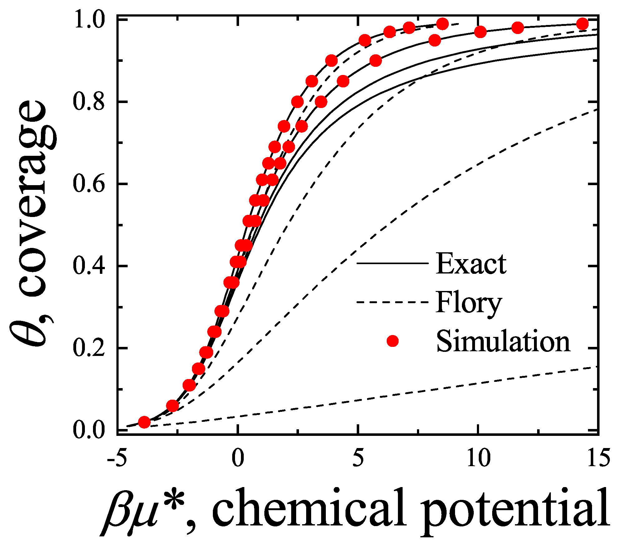
Figure 2.
Molar entropy (in units of ) versus surface coverage. Comparison between exact results (solid line) and Flory-Huggins’s approach (dashed line) for monomers (), dimers () and polymers ( and ). Curves from top to bottom (the case is common for both results).
Figure 2.
Molar entropy (in units of ) versus surface coverage. Comparison between exact results (solid line) and Flory-Huggins’s approach (dashed line) for monomers (), dimers () and polymers ( and ). Curves from top to bottom (the case is common for both results).
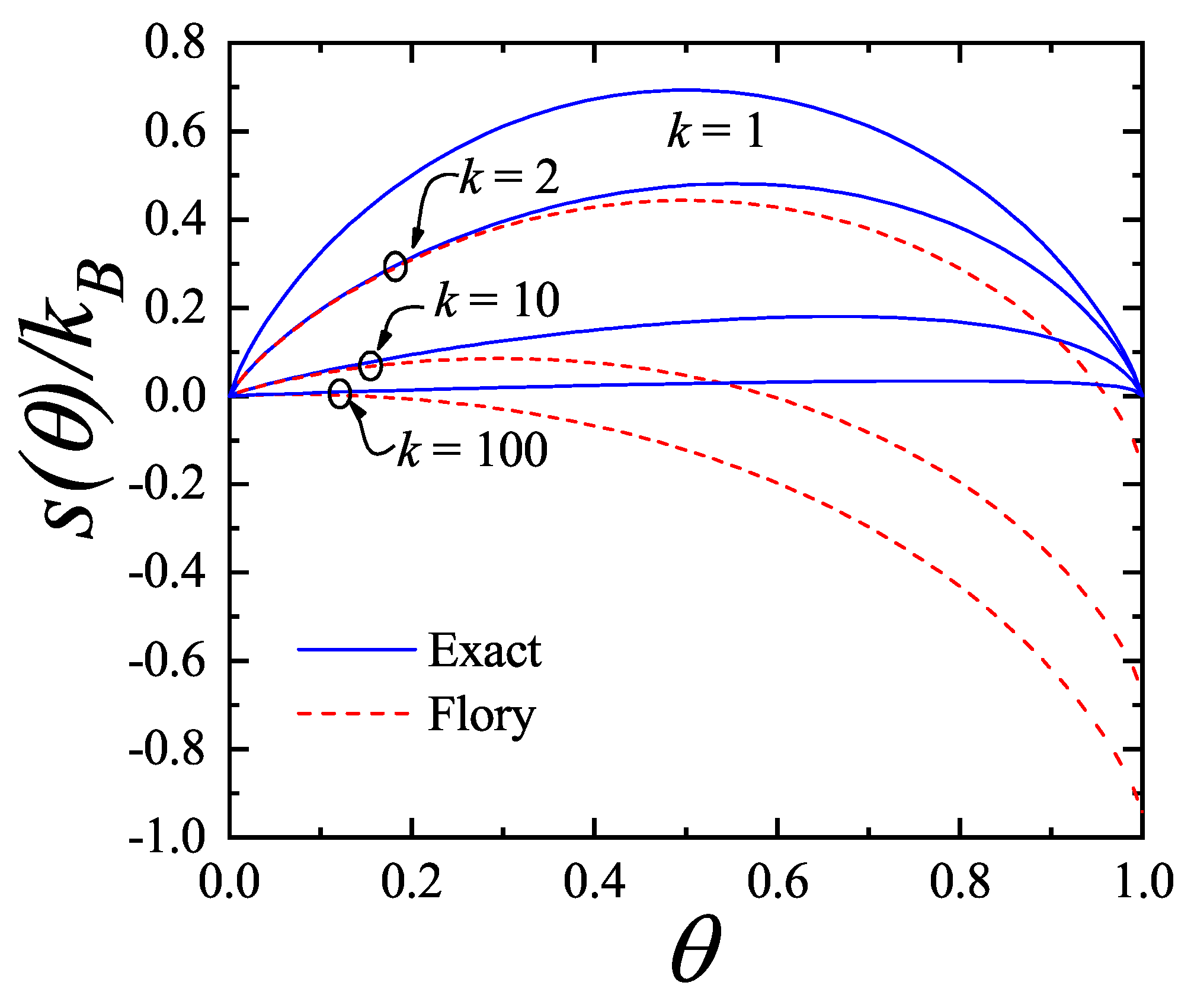
Figure 3.
Spreading pressure in units of versus surface coverage. Comparison between exact results (solid line) and Flory-Huggins’s approach (dashed line) for monomers (), dimers () and polymers ( and ). Curves from top to bottom (the case is common for both results).
Figure 3.
Spreading pressure in units of versus surface coverage. Comparison between exact results (solid line) and Flory-Huggins’s approach (dashed line) for monomers (), dimers () and polymers ( and ). Curves from top to bottom (the case is common for both results).
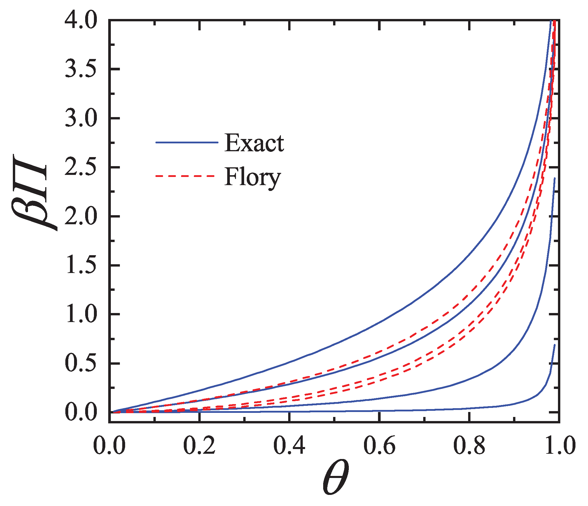
Figure 4.
Total and partial adsorption isotherms for a monomer-dimer binary mixture adsorbed on a one-dimensional lattice with and . Symbols and solid lines represent MC and theoretical data, respectively.
Figure 4.
Total and partial adsorption isotherms for a monomer-dimer binary mixture adsorbed on a one-dimensional lattice with and . Symbols and solid lines represent MC and theoretical data, respectively.
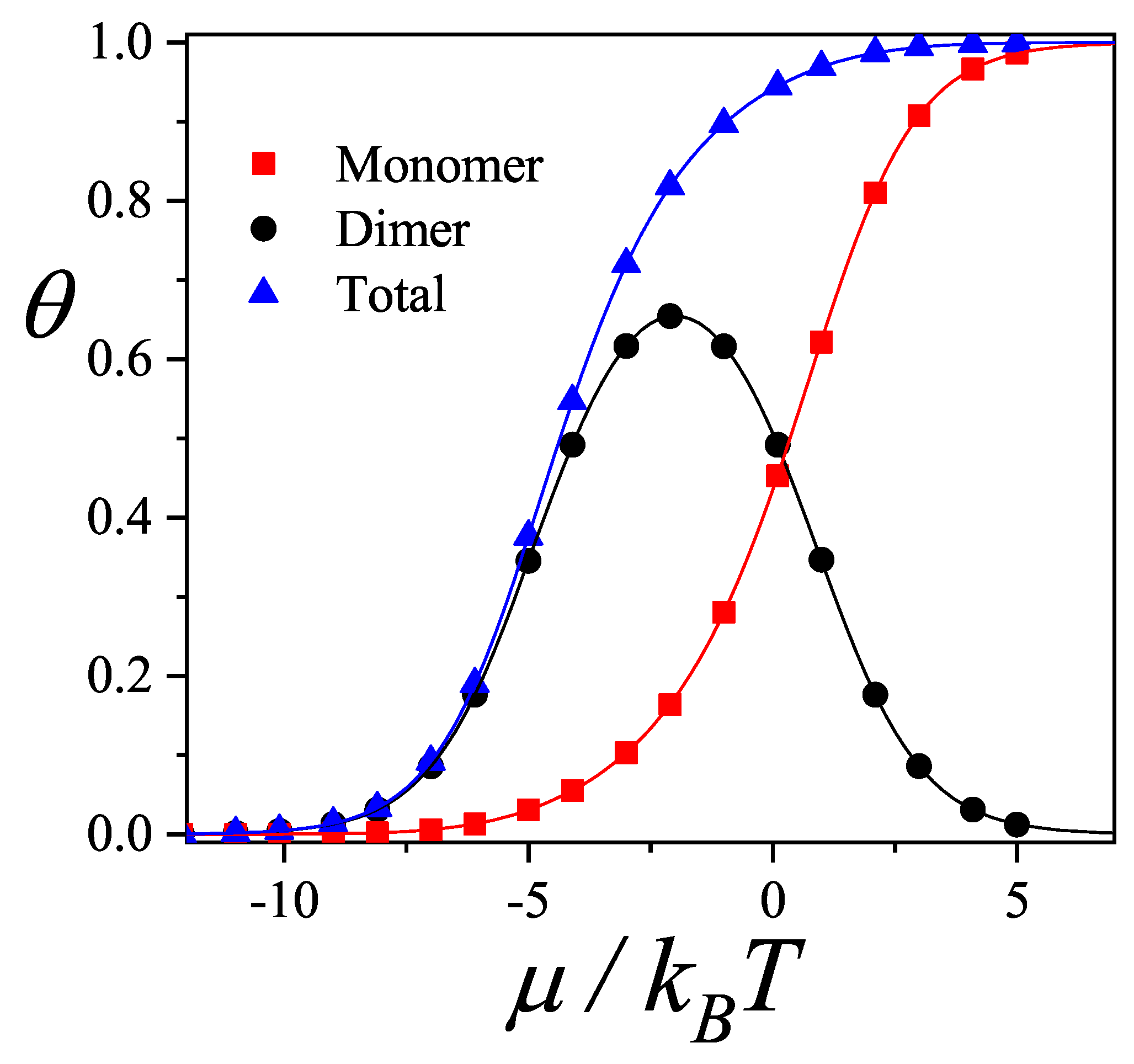
Figure 5.
Cartoon representing the lattice gas model of k-mer adsorption in the multilayer regime (the case of trimer adsorption is depicted). Adsorption sites are represented by crosses on the adsorbent’s surface. The adsorbate molecule is represented by black beds connected by solid bonds.
Figure 5.
Cartoon representing the lattice gas model of k-mer adsorption in the multilayer regime (the case of trimer adsorption is depicted). Adsorption sites are represented by crosses on the adsorbent’s surface. The adsorbate molecule is represented by black beds connected by solid bonds.
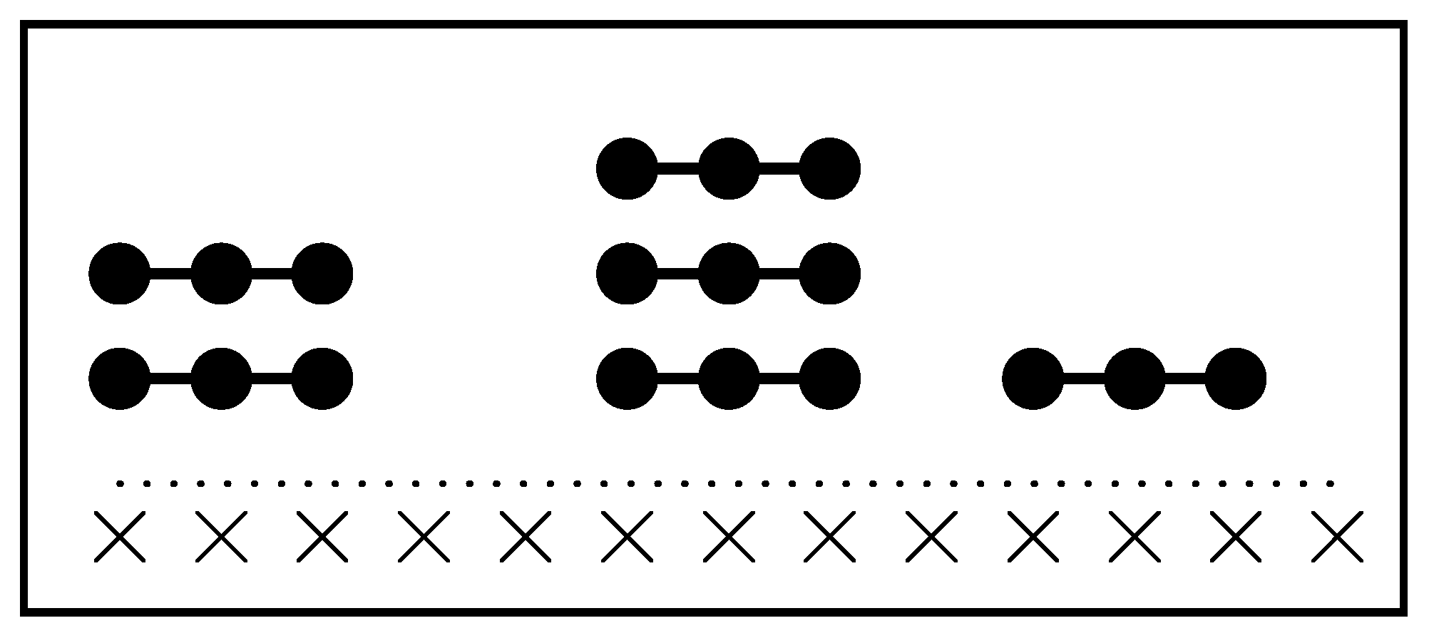
Figure 6.
Adsorption isotherms for different values of the parameter c. The solid line represents the isotherm for dimers obtained in the present work [Equation (60)], and the dashed line does for the BET’s isotherm (monomers). The pairs of curves from bottom to top correspond to and 100, in the range of in Figure 6a) and of in Figure 6b).
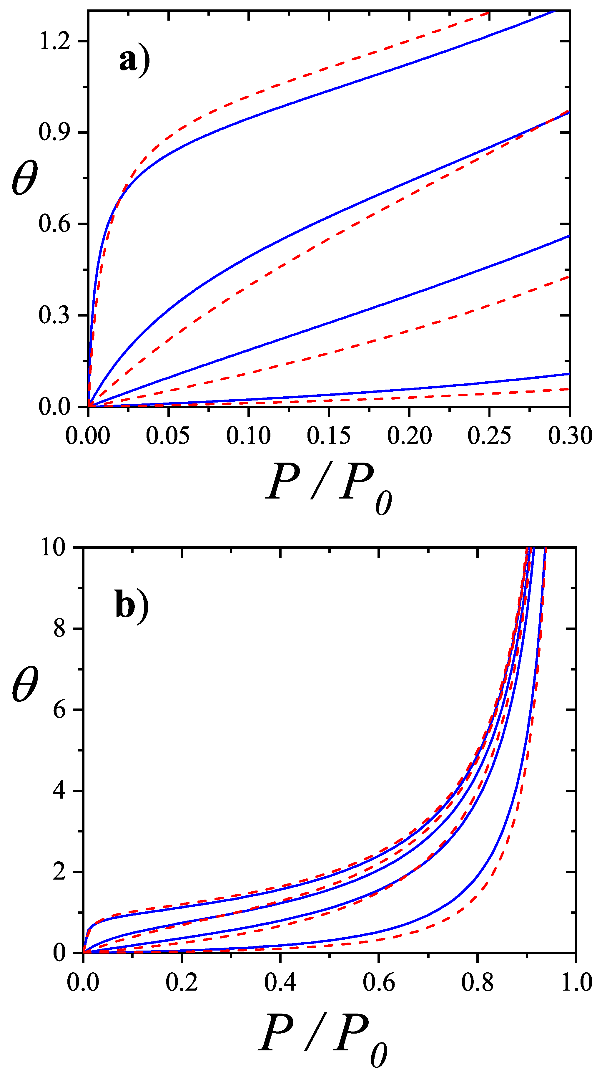
Figure 7.
versus for (in arbitrary units), and (curves from bottom to top). Solid and dashed curves represent the same models as in Figure 6.
Figure 7.
versus for (in arbitrary units), and (curves from bottom to top). Solid and dashed curves represent the same models as in Figure 6.
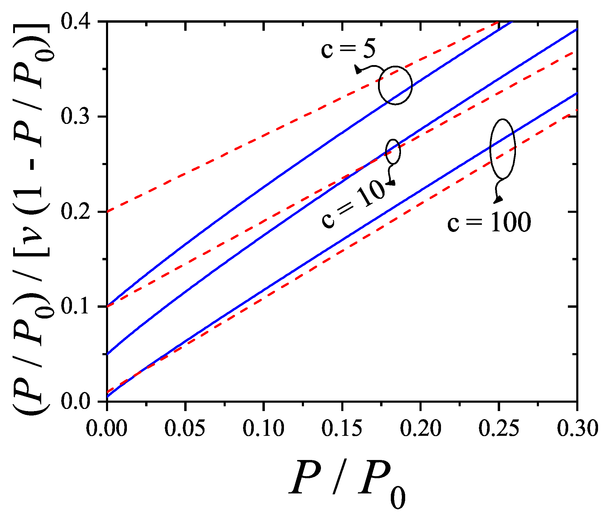
Figure 8.
Adsorption isotherms for interacting (repulsive as well attractive) dimers and 10-mers; (a) , ; (b) , ; (c) , ; (d) , . The full circles represent results from Monte Carlo Simulation in the lattice-gas model. Comparison between experimental isotherm of CH4 from Ref. [64] (open triangles, K; open diamonds, K) and theoretical isotherm [from Equation (73)] of dimers in the lattice-gas approximation (full triangles, K, Kcal/mol; full diamonds K, Kcal/mol).
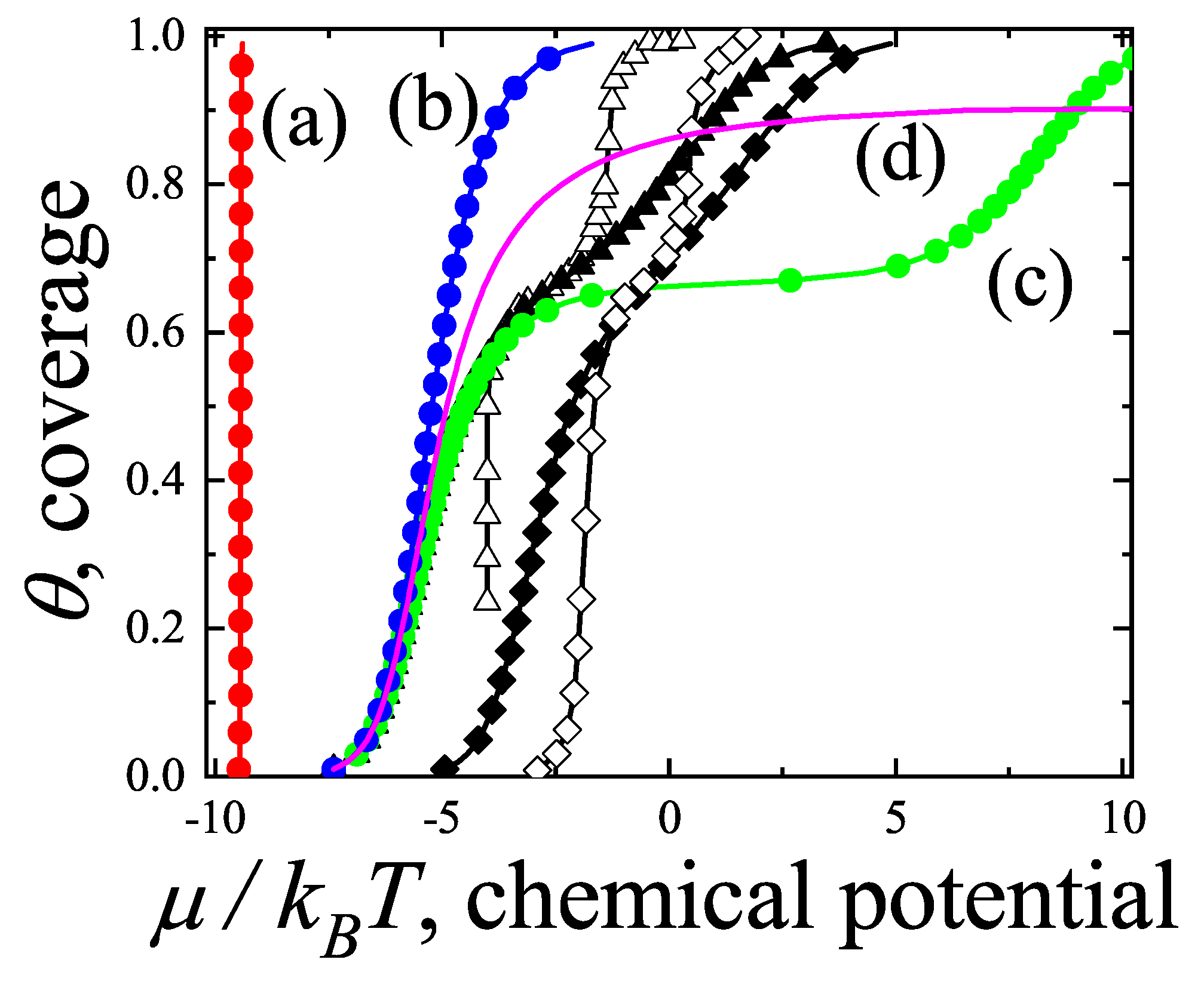
Figure 9.
Entropy per site, , versus lattice coverage, , for interacting (repulsive as well attractive) dimers and 10-mers; (a) , ; (b) , , (c) , ; (d) , ; (e) , ; (f) , . Symbols and lines represent MC simulation data and theoretical results, respectively.
Figure 9.
Entropy per site, , versus lattice coverage, , for interacting (repulsive as well attractive) dimers and 10-mers; (a) , ; (b) , , (c) , ; (d) , ; (e) , ; (f) , . Symbols and lines represent MC simulation data and theoretical results, respectively.
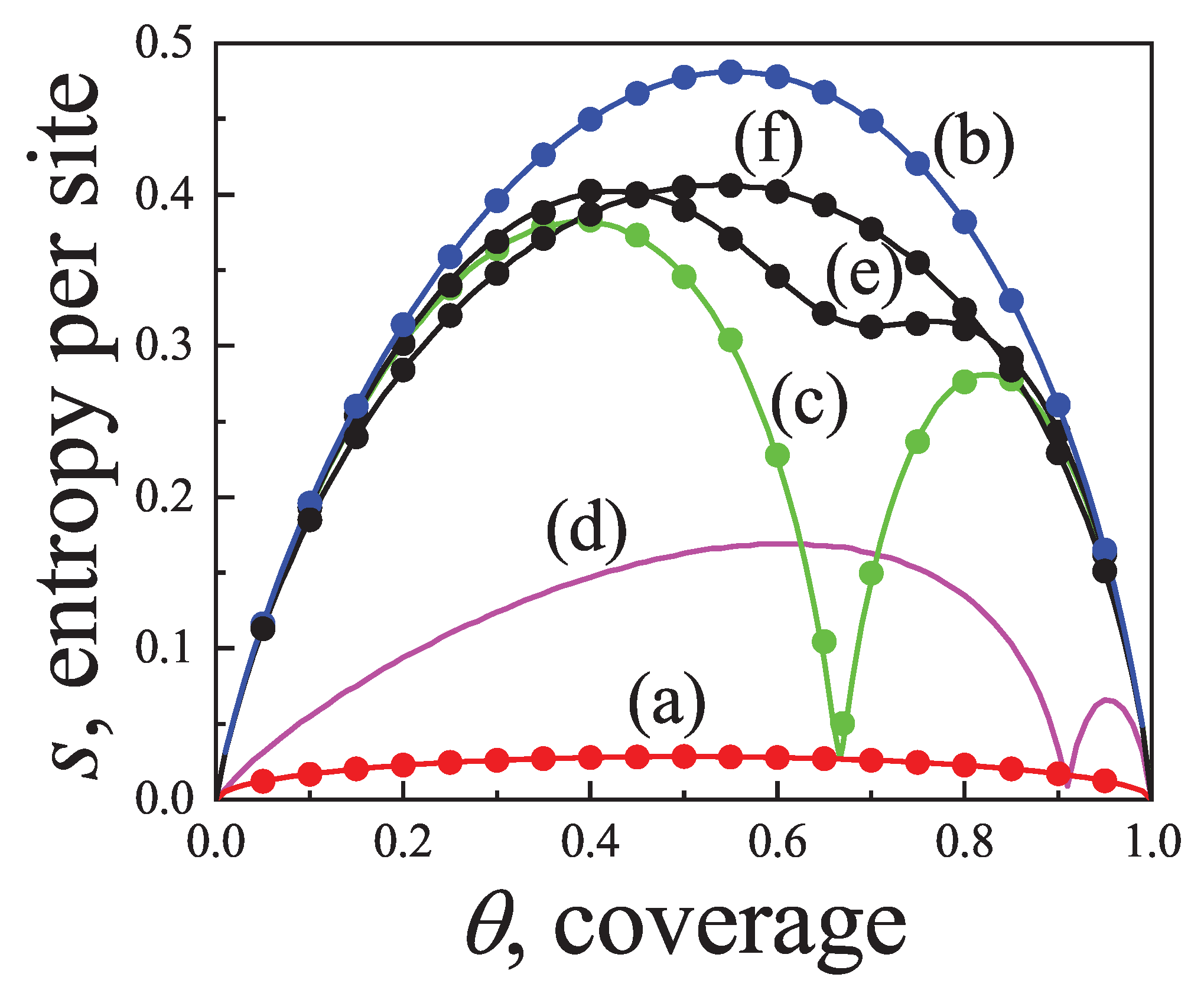
Figure 10.
Specific heat in units of (at constants volume) versus at . (a) monomers (); (b) dimers (); (c) trimers (); (d) 10-mers (). The cases (a) and (b) correspond to the left hand side axis and the cases (c) and (d) correspond to the right hand side axis.
Figure 10.
Specific heat in units of (at constants volume) versus at . (a) monomers (); (b) dimers (); (c) trimers (); (d) 10-mers (). The cases (a) and (b) correspond to the left hand side axis and the cases (c) and (d) correspond to the right hand side axis.
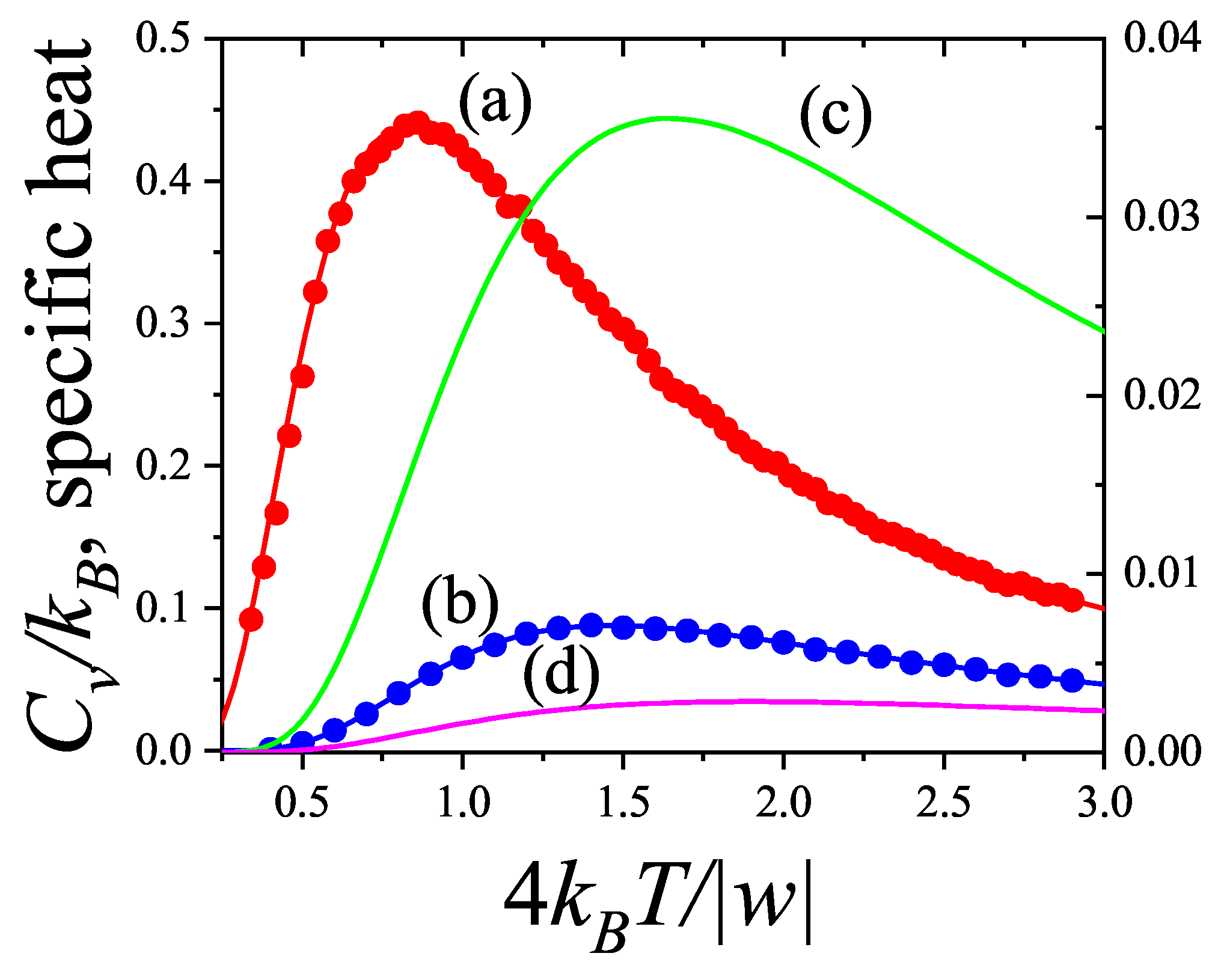
Figure 11.
Schematic representation of a lattice-gas of dimers (, blue circles) and trimers (, red circles) adsorbed on a one-dimensional lattice. The figure shows different types of pairs of sites: a) 00, b) , c) , d) , e) and f) .
Figure 11.
Schematic representation of a lattice-gas of dimers (, blue circles) and trimers (, red circles) adsorbed on a one-dimensional lattice. The figure shows different types of pairs of sites: a) 00, b) , c) , d) , e) and f) .
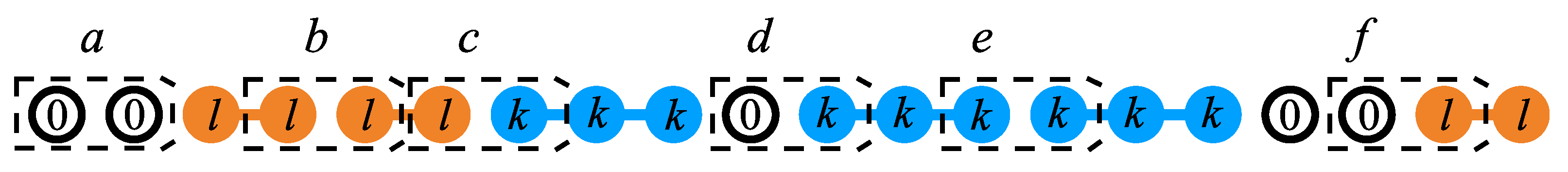
Figure 12.
Rules for the mapping , from the original lattice of polyatomics to an effective lattice of monomers .
Figure 12.
Rules for the mapping , from the original lattice of polyatomics to an effective lattice of monomers .
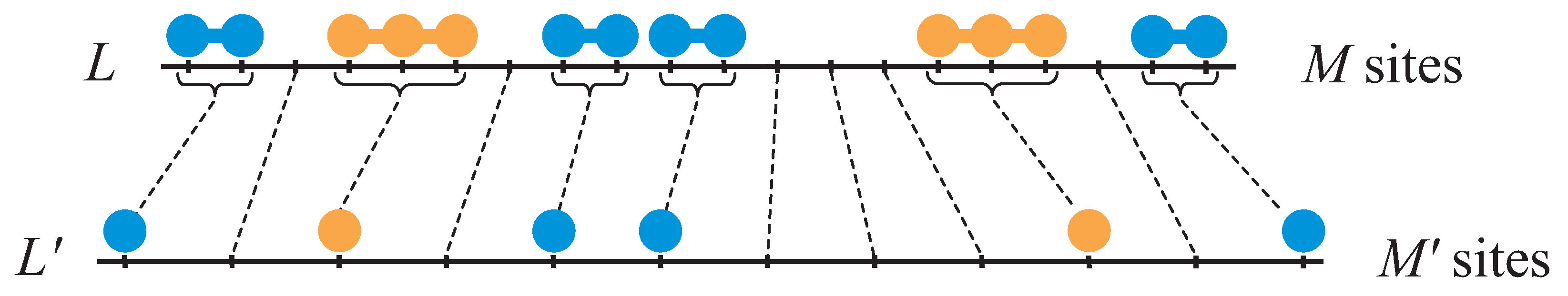
Figure 13.
Partial adsorption isotherms for the 1D case, , and different values of the lateral interaction as indicated. Symbols correspond to MC data whereas lines represent the theoretical results.
Figure 13.
Partial adsorption isotherms for the 1D case, , and different values of the lateral interaction as indicated. Symbols correspond to MC data whereas lines represent the theoretical results.
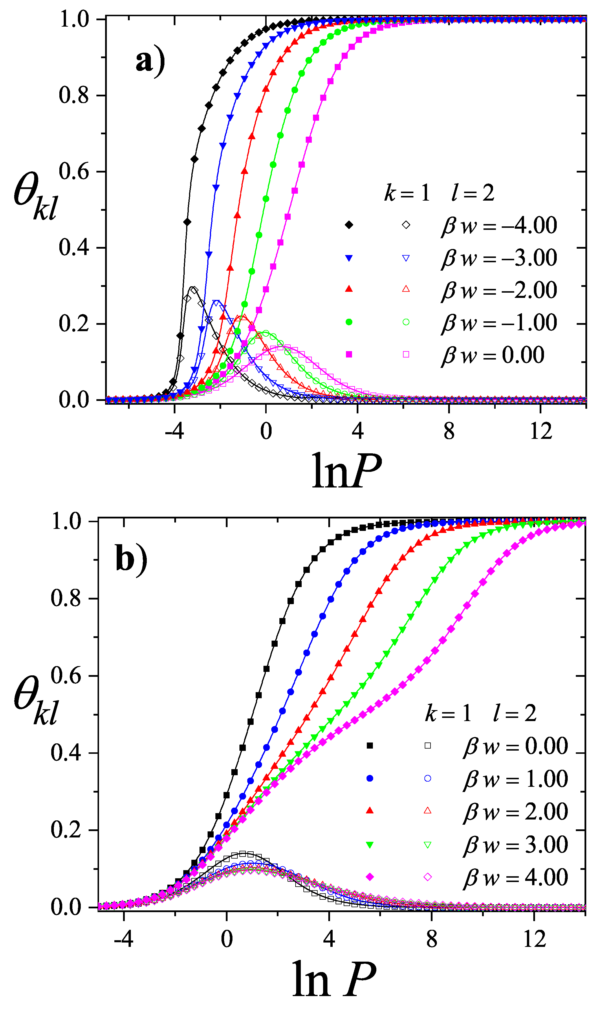
Figure 14.
Linear tetramers adsorbed on (a) square, (b) triangular and (c) honeycomb lattices. Full and empty circles represent tetramer units and empty sites, respectively.
Figure 14.
Linear tetramers adsorbed on (a) square, (b) triangular and (c) honeycomb lattices. Full and empty circles represent tetramer units and empty sites, respectively.
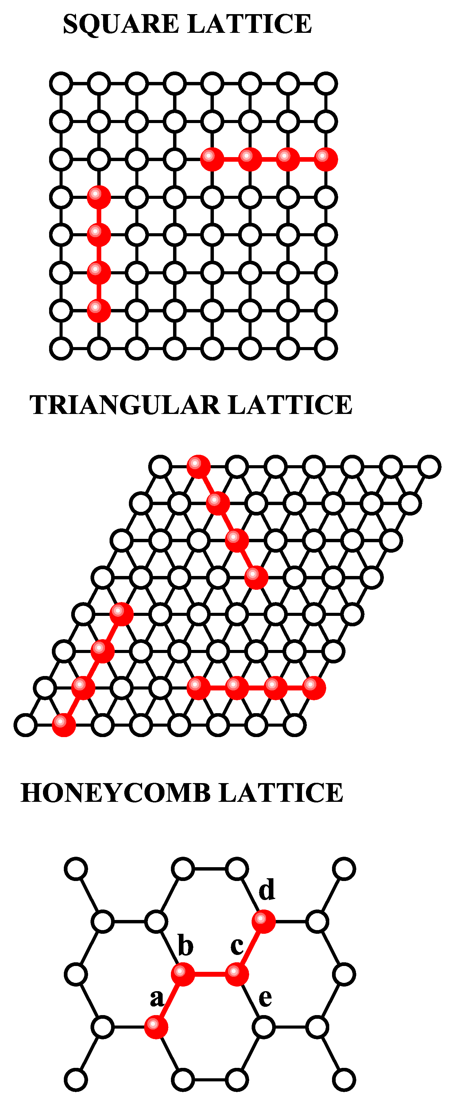
Figure 15.
Schematic representation of a lattice-gas of dimers (, blue circles) and trimers (, red circles) adsorbed on a square lattice (). The figure shows different types of pairs of sites: a) , b) , c) , d) 00, e) and f) .
Figure 15.
Schematic representation of a lattice-gas of dimers (, blue circles) and trimers (, red circles) adsorbed on a square lattice (). The figure shows different types of pairs of sites: a) , b) , c) , d) 00, e) and f) .
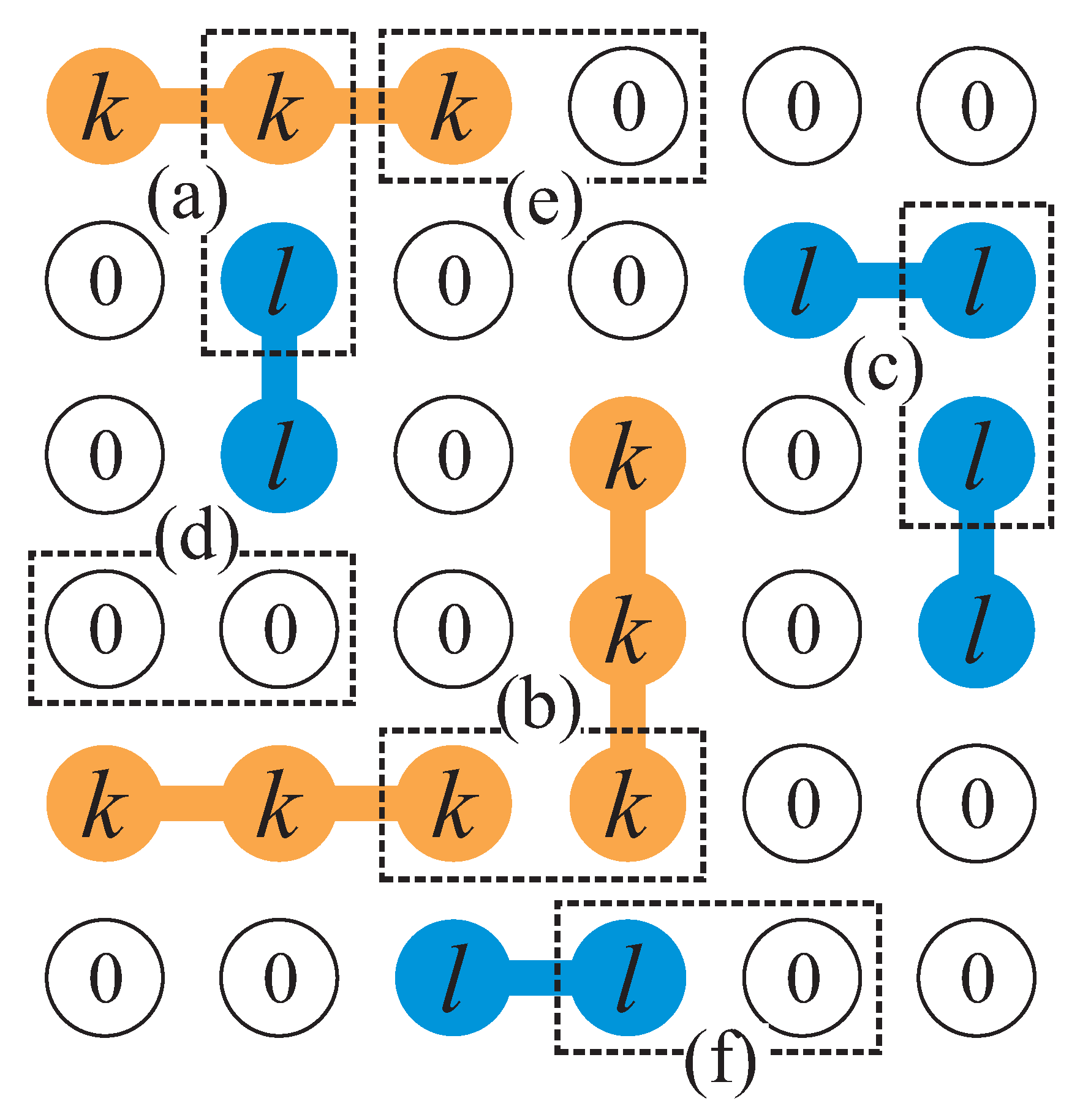
Figure 16.
Entropy per site vs. lattice coverage for . Dashed lines: isotropic phase (I). Solid lines: fully aligned nematic phase (N). First-order approximation through Equations (285), (294), (300).
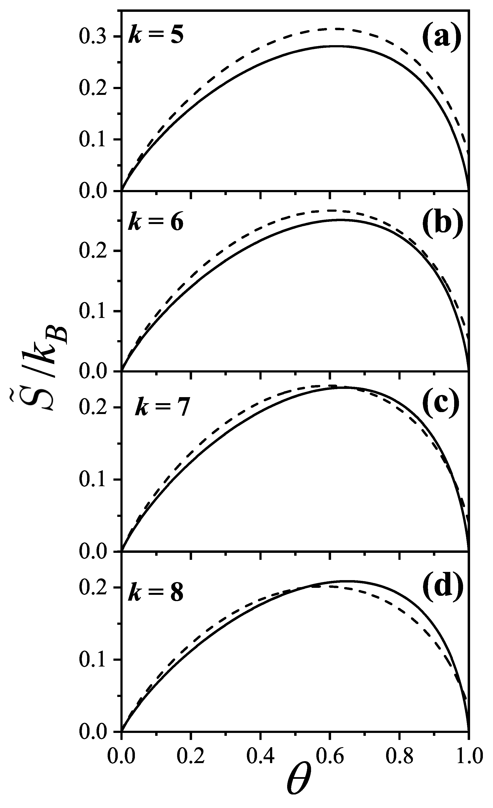
Figure 17.
Critical coverages (lower branch) and (upper branch) as functions of k. Open squares: first-order approximation. Solid squares: second-order approximation.
Figure 17.
Critical coverages (lower branch) and (upper branch) as functions of k. Open squares: first-order approximation. Solid squares: second-order approximation.
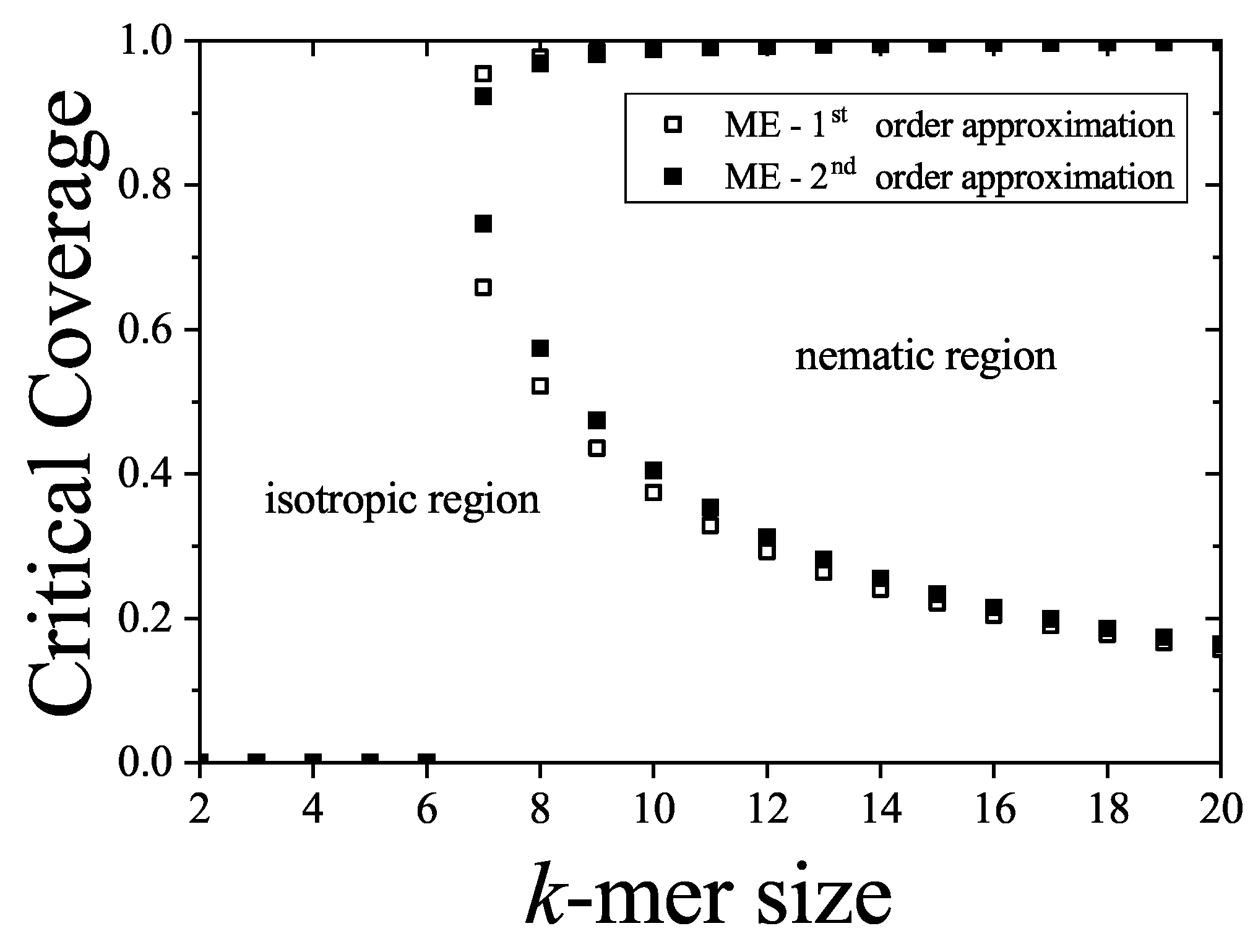
Figure 18.
Entropy per site vs. lattice coverage for and 8. Symbols: MC data [109]. Dashed: model (isotropic phase) with (), (). Solid: result for nematic phase (). Dotted: empirical correction . Inset: high coverage behavior for .
Figure 18.
Entropy per site vs. lattice coverage for and 8. Symbols: MC data [109]. Dashed: model (isotropic phase) with (), (). Solid: result for nematic phase (). Dotted: empirical correction . Inset: high coverage behavior for .
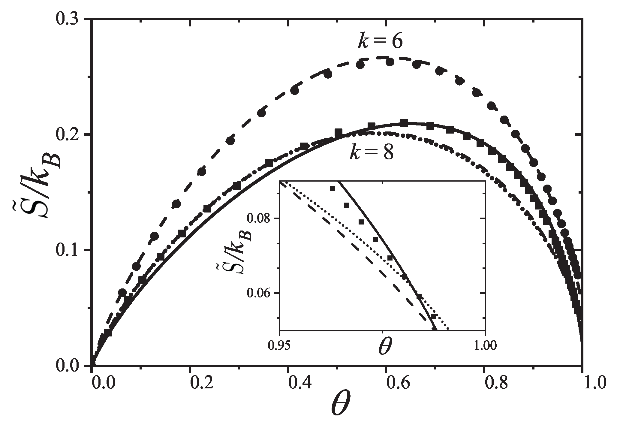
Figure 19.
Lattice coverage versus for k-mers on a square lattice. : , , , (dashed line), (solid line); : , , , (dotted line). Symbols denote MC simulation results: squares for , circles for .
Figure 19.
Lattice coverage versus for k-mers on a square lattice. : , , , (dashed line), (solid line); : , , , (dotted line). Symbols denote MC simulation results: squares for , circles for .
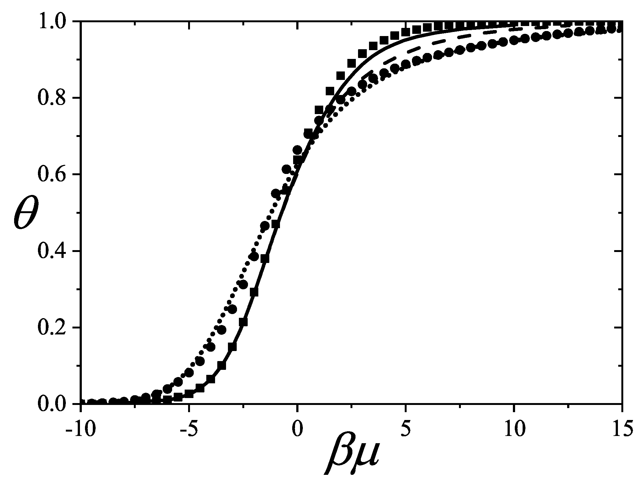
Figure 20.
Exclusion spectrum function vs. lattice coverage . Lines: theory from Equation (291); dot-dashed (), dashed (), solid ( rectangles), dotted ( squares). Symbols: MC data as indicated.
Figure 20.
Exclusion spectrum function vs. lattice coverage . Lines: theory from Equation (291); dot-dashed (), dashed (), solid ( rectangles), dotted ( squares). Symbols: MC data as indicated.
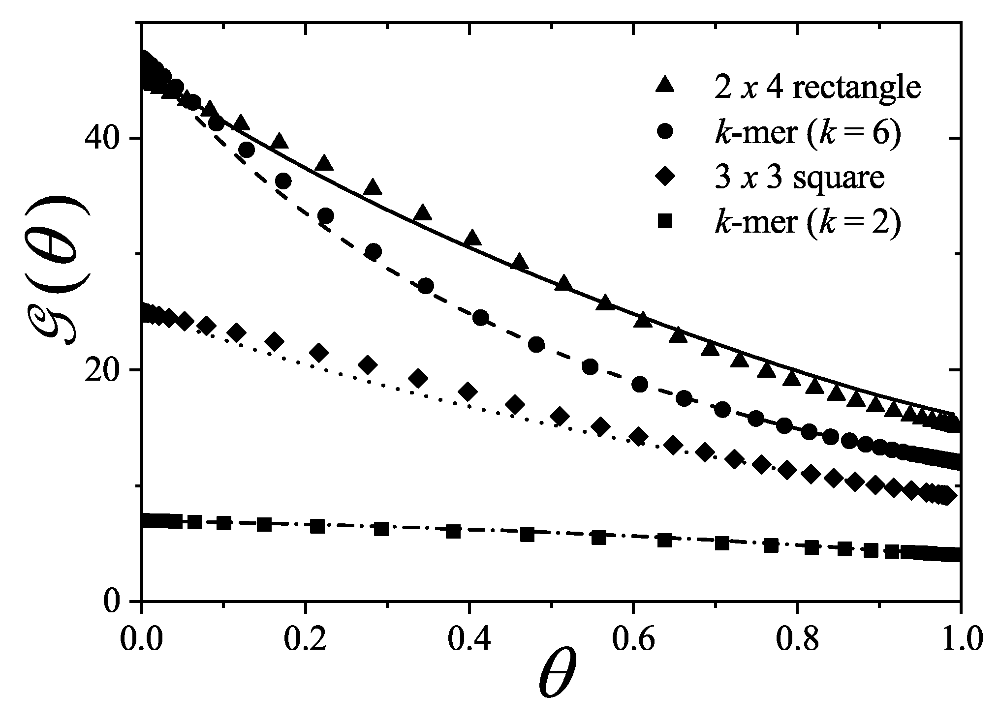
Figure 21.
Same as Figure 20, but for the exclusion per particle frequency function .
Figure 21.
Same as Figure 20, but for the exclusion per particle frequency function .

Figure 22.
A schematic representation of a ternary mixture: a tetramer (blue), a dimer (red), and a monomer (green). The dotted lines indicate examples of multiply excluded states within the spectrum of (a) tetramers, (b) dimers due to tetramers and monomers, and (c) dimers via self-exclusion. This emphasizes the multiplicity of state exclusions even at finite densities.
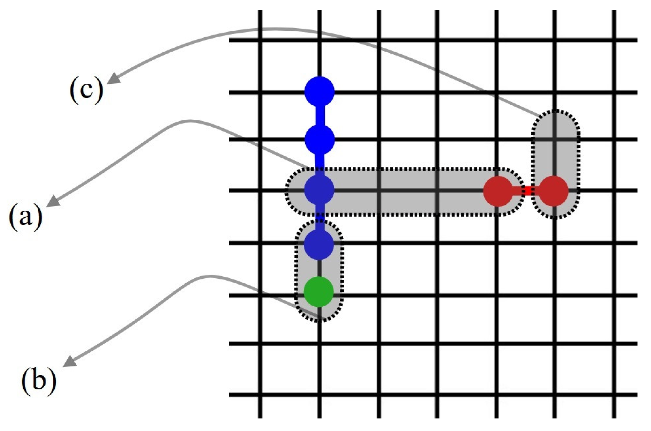
Figure 24.
Comparison between the exact adsorption isotherm of monomers and the simulation adsorption isotherms of dimers on honeycomb, square and triangular lattices.
Figure 24.
Comparison between the exact adsorption isotherm of monomers and the simulation adsorption isotherms of dimers on honeycomb, square and triangular lattices.
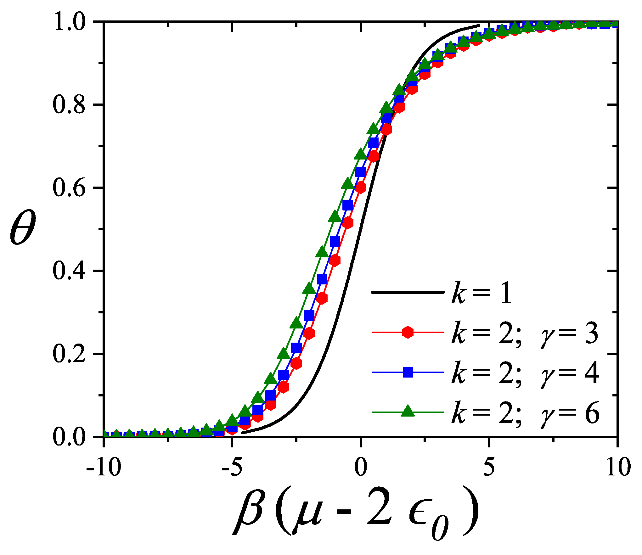
Figure 25.
Adsorption isotherms of 6-mers on a honeycomb lattice. Symbols represent MC results, and lines correspond to different approaches (see inset). Percentage reduced coverage, , versus surface coverage. The symbols are as in part .
Figure 25.
Adsorption isotherms of 6-mers on a honeycomb lattice. Symbols represent MC results, and lines correspond to different approaches (see inset). Percentage reduced coverage, , versus surface coverage. The symbols are as in part .
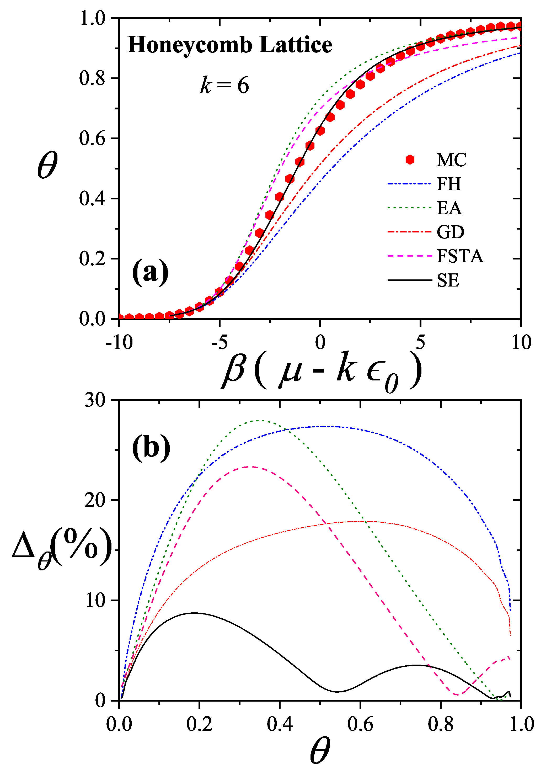
Figure 26.
As Figure 5 for a square lattice.
Figure 26.
As Figure 5 for a square lattice.
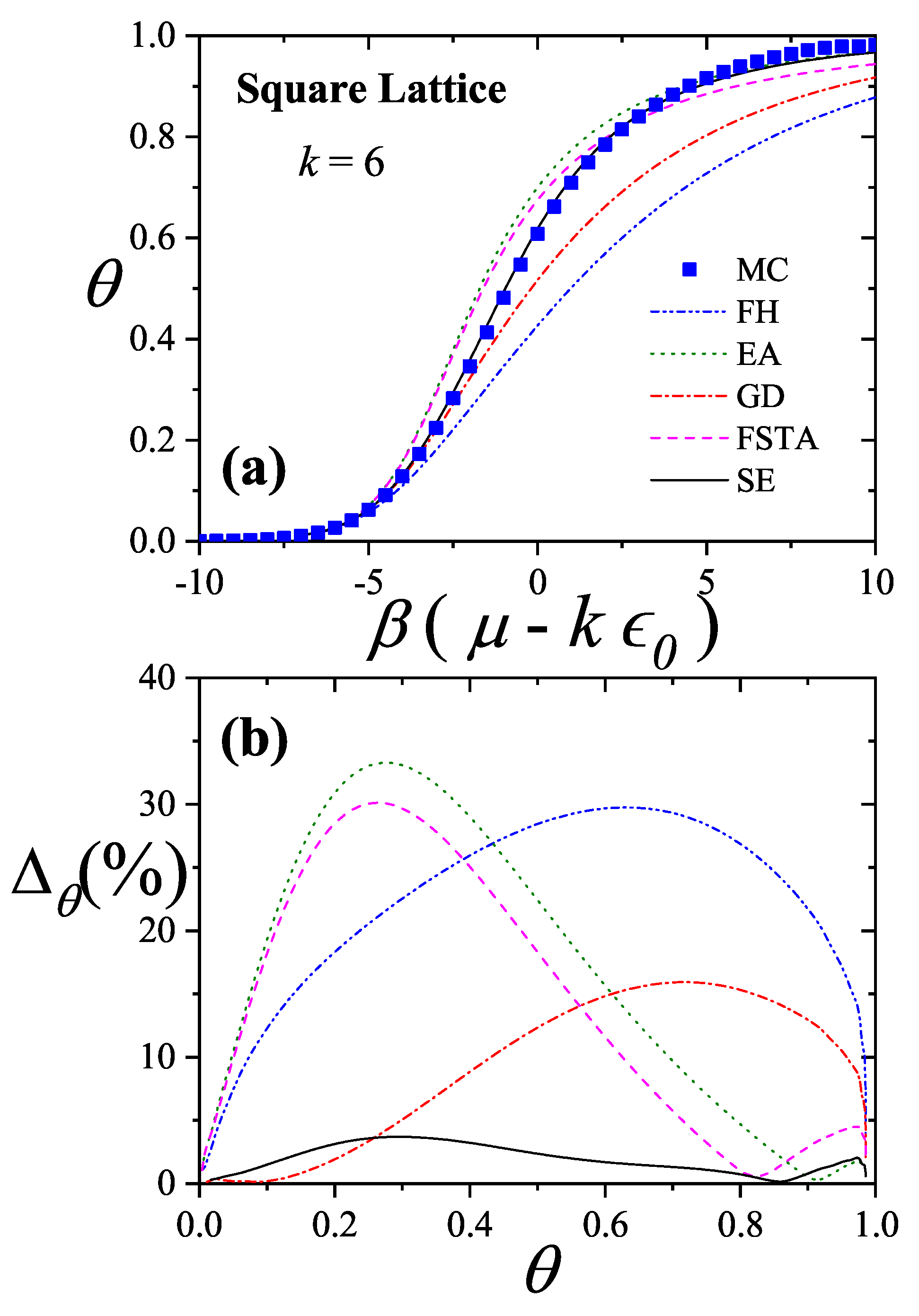
Figure 27.
As Figure 5 for a triangular lattice.
Figure 27.
As Figure 5 for a triangular lattice.
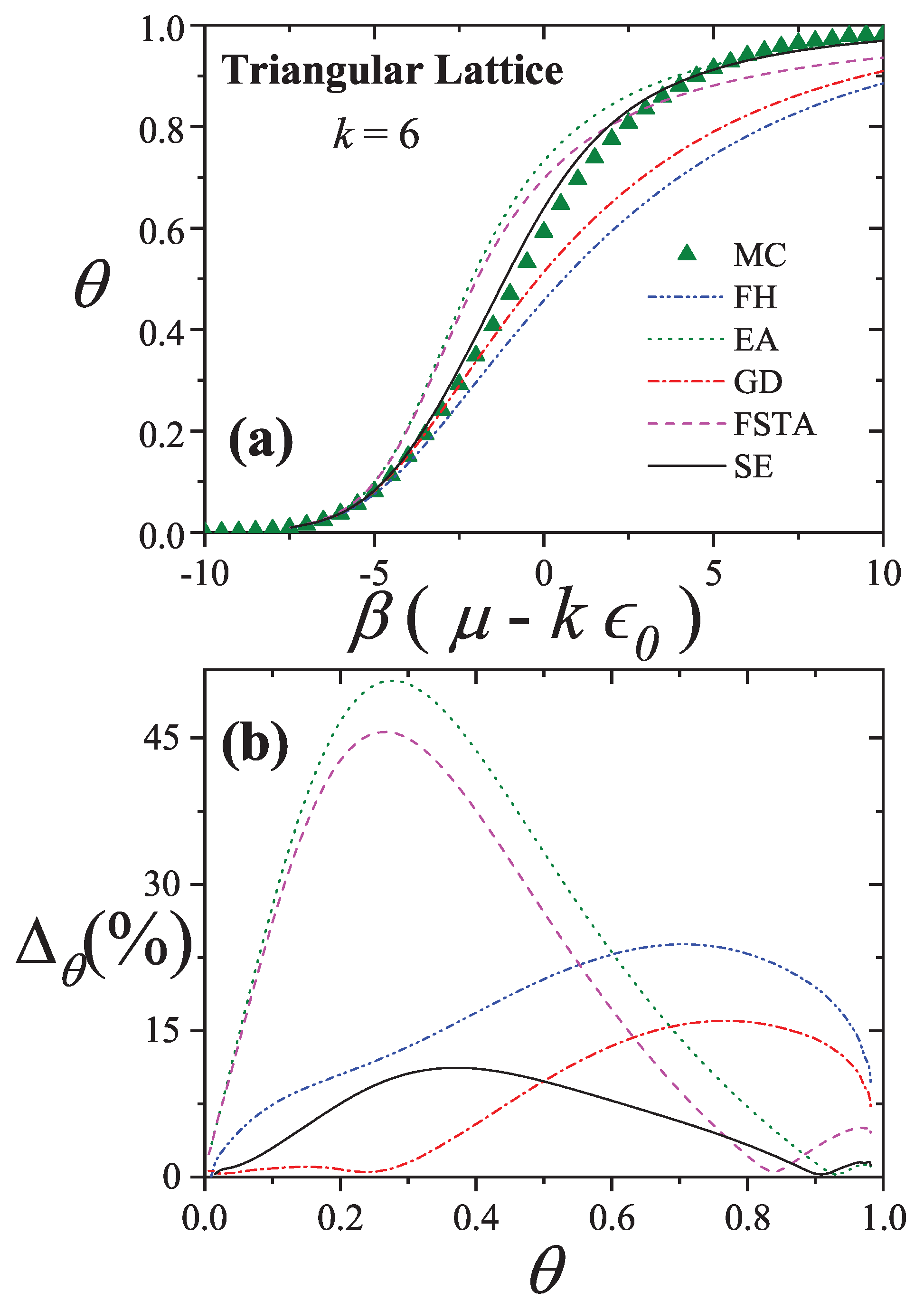
Figure 28.
Percentage reduced coverage versus concentration for k-mers adsorbed on a honeycomb lattice and approximation. Symbols are indicated in the inset.
Figure 28.
Percentage reduced coverage versus concentration for k-mers adsorbed on a honeycomb lattice and approximation. Symbols are indicated in the inset.
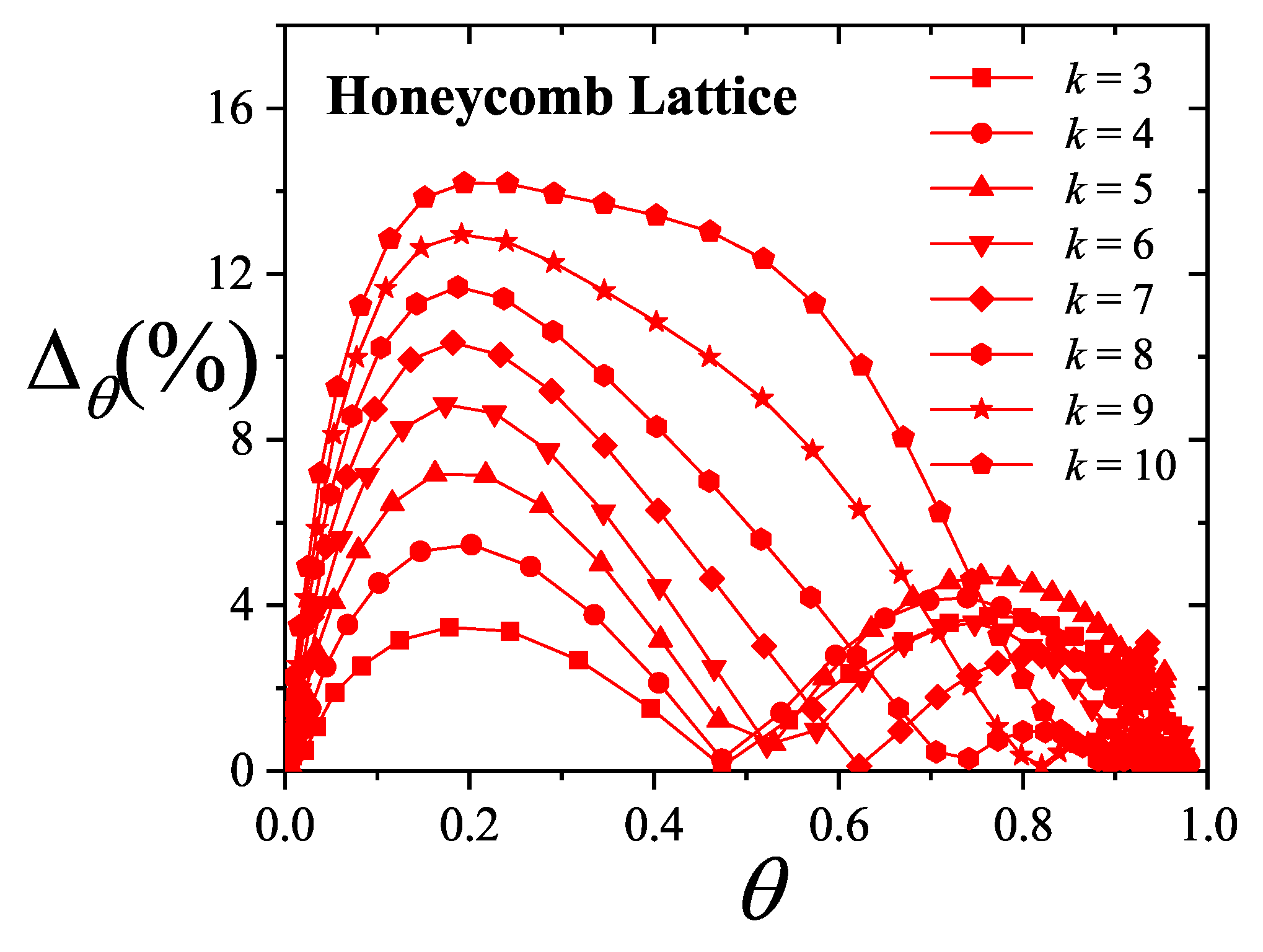
Figure 29.
As Figure 28 for a square lattice.
Figure 29.
As Figure 28 for a square lattice.
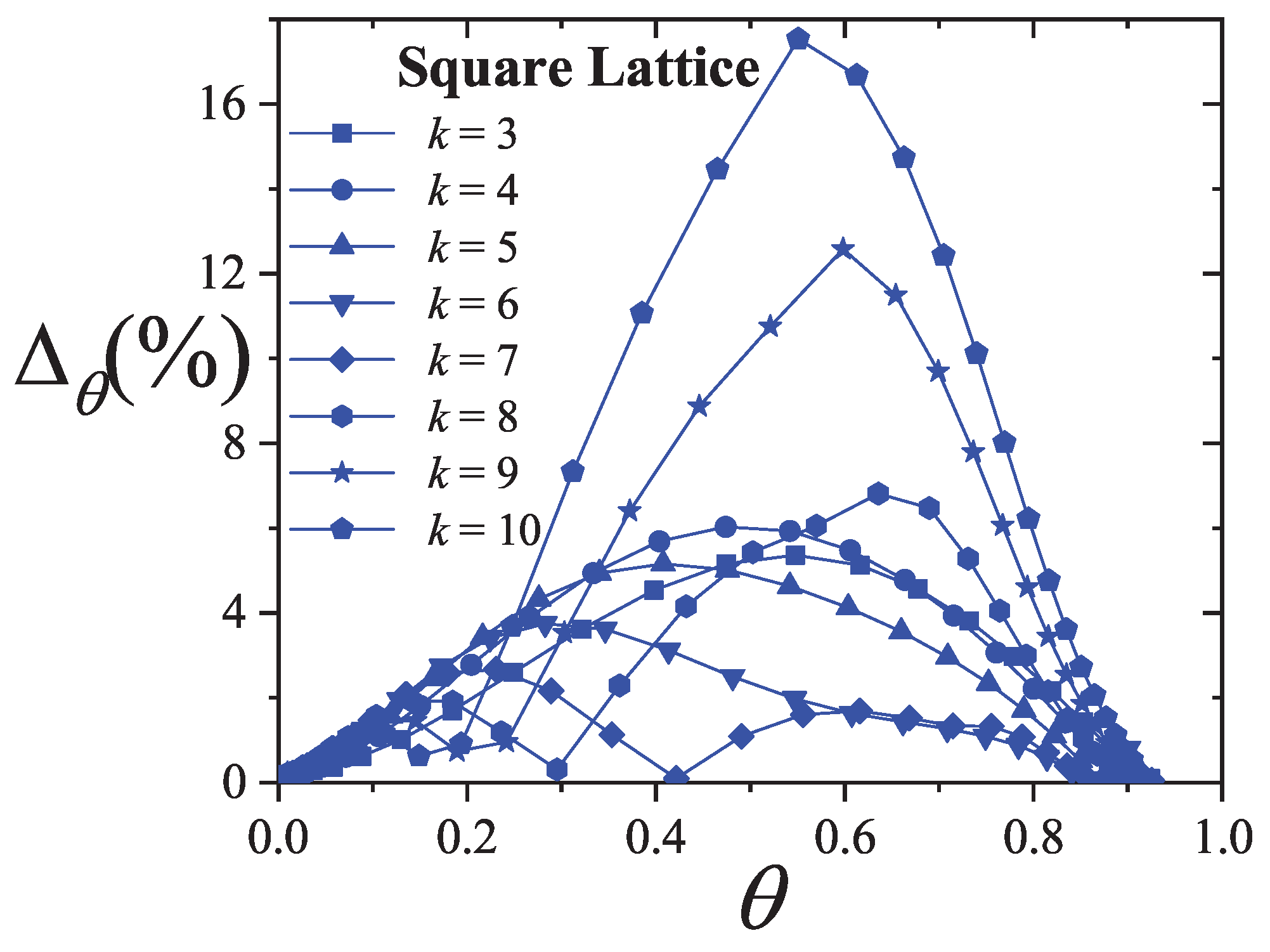
Figure 30.
As Figure 28 for a triangular lattice.
Figure 30.
As Figure 28 for a triangular lattice.
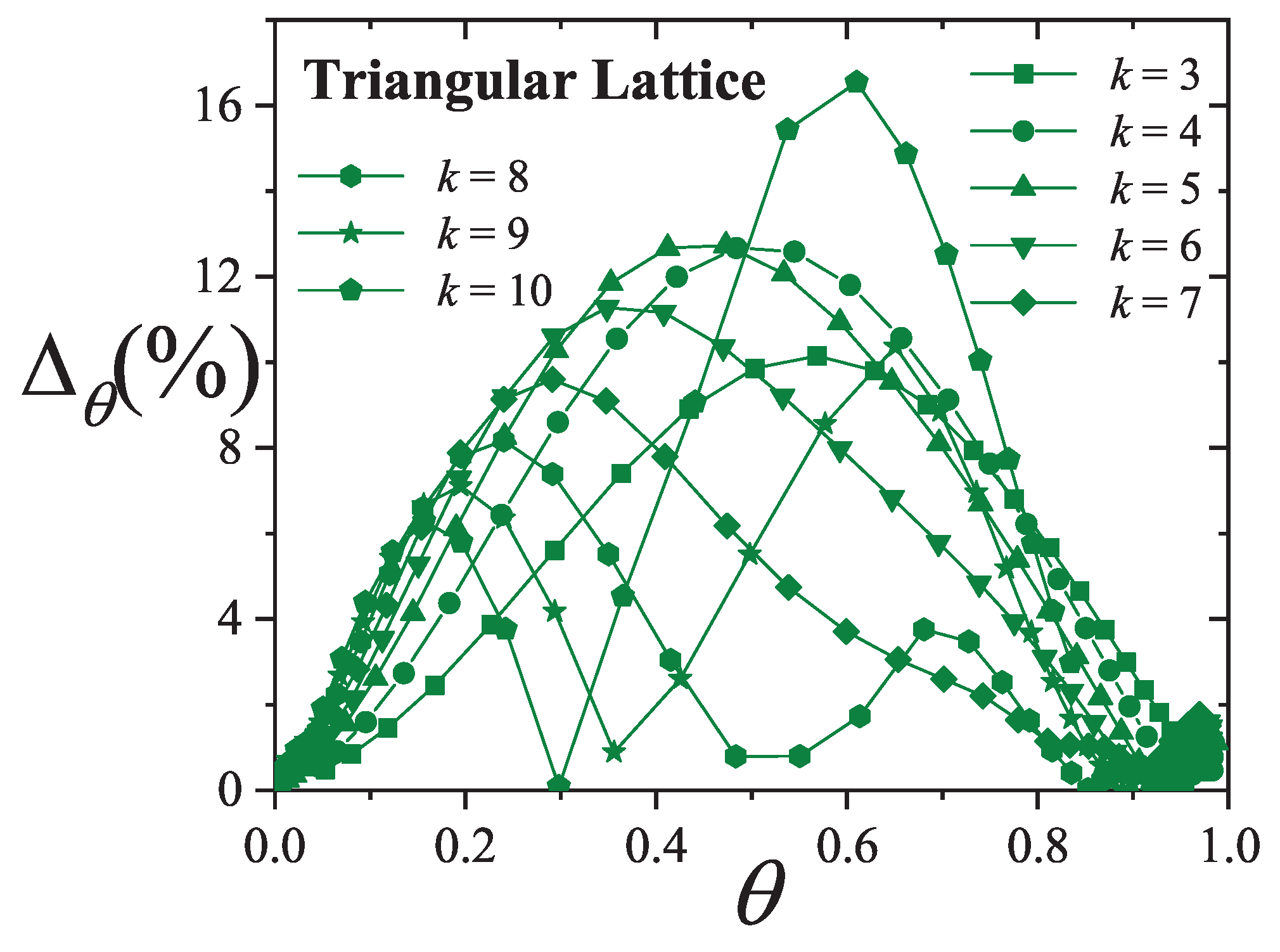
Figure 31.
a) Average percentage reduced coverage , as a function of k for different connectivities. b) As in part a) for the maximum percentage reduced coverage . Hexagons, squares and triangles correspond to data obtained for honeycomb, square an triangular lattices, respectively.
Figure 31.
a) Average percentage reduced coverage , as a function of k for different connectivities. b) As in part a) for the maximum percentage reduced coverage . Hexagons, squares and triangles correspond to data obtained for honeycomb, square an triangular lattices, respectively.
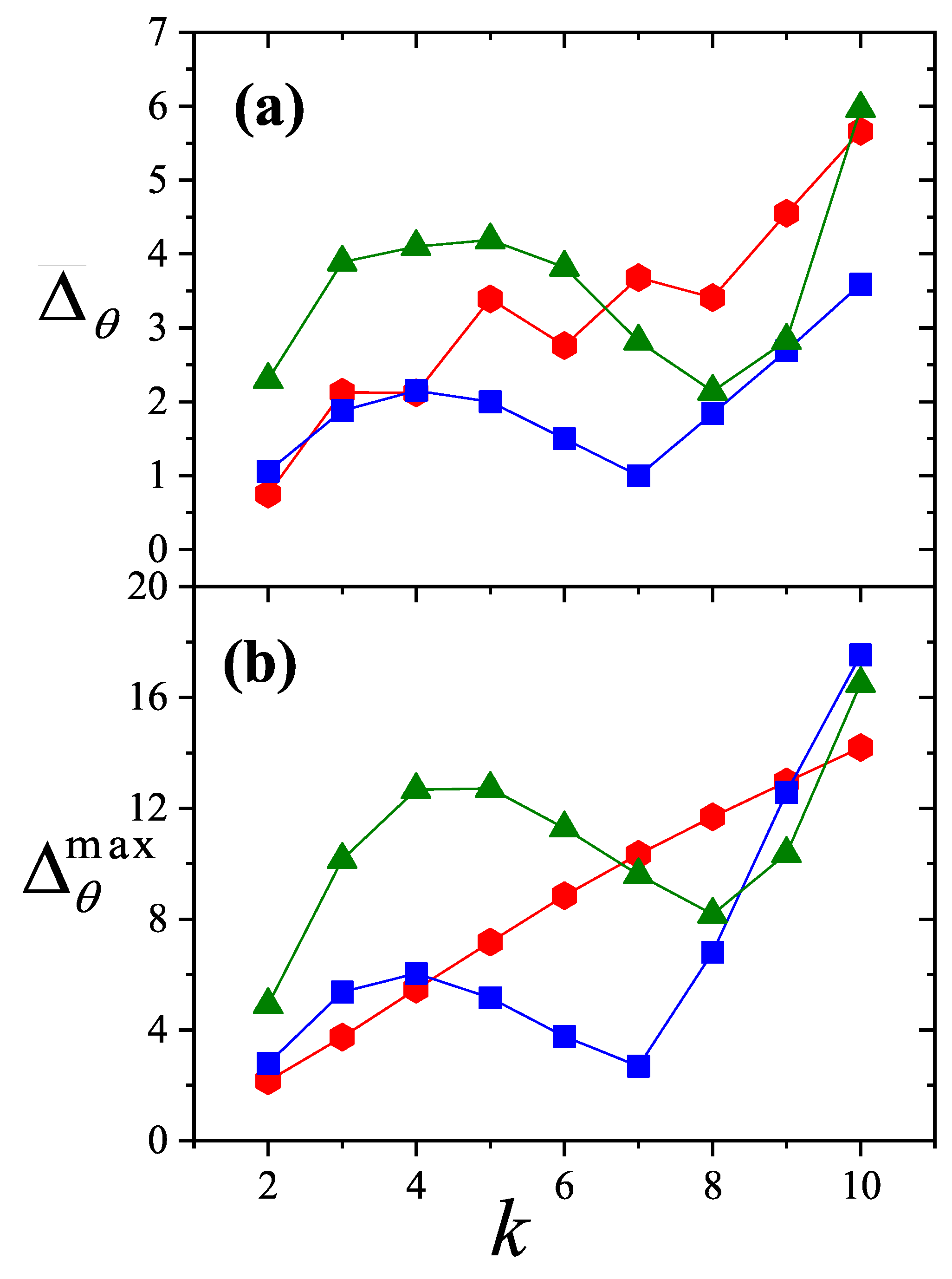
Figure 32.
Adsorption isotherms for rigid molecules on a square lattice: (a) and ; (b) and . (c)[(d)] Reduced coverage error vs. the total surface coverage for the data in part (a)[(b)]. Symbols represent MC results, and lines correspond to different theoretical approaches as indicated.
Figure 32.
Adsorption isotherms for rigid molecules on a square lattice: (a) and ; (b) and . (c)[(d)] Reduced coverage error vs. the total surface coverage for the data in part (a)[(b)]. Symbols represent MC results, and lines correspond to different theoretical approaches as indicated.
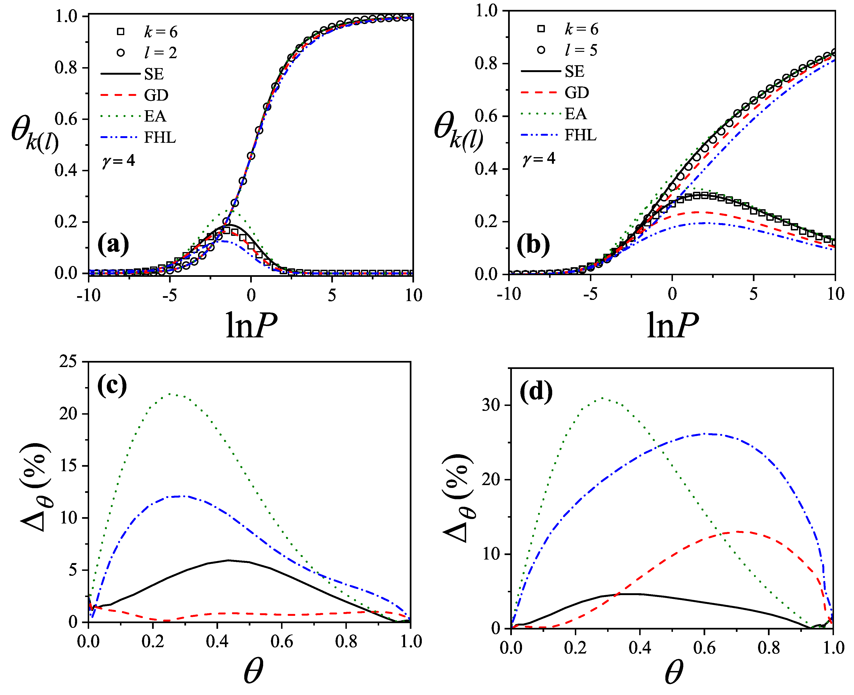
Figure 33.
Same as Figure 32 for triangular lattices.
Figure 33.
Same as Figure 32 for triangular lattices.
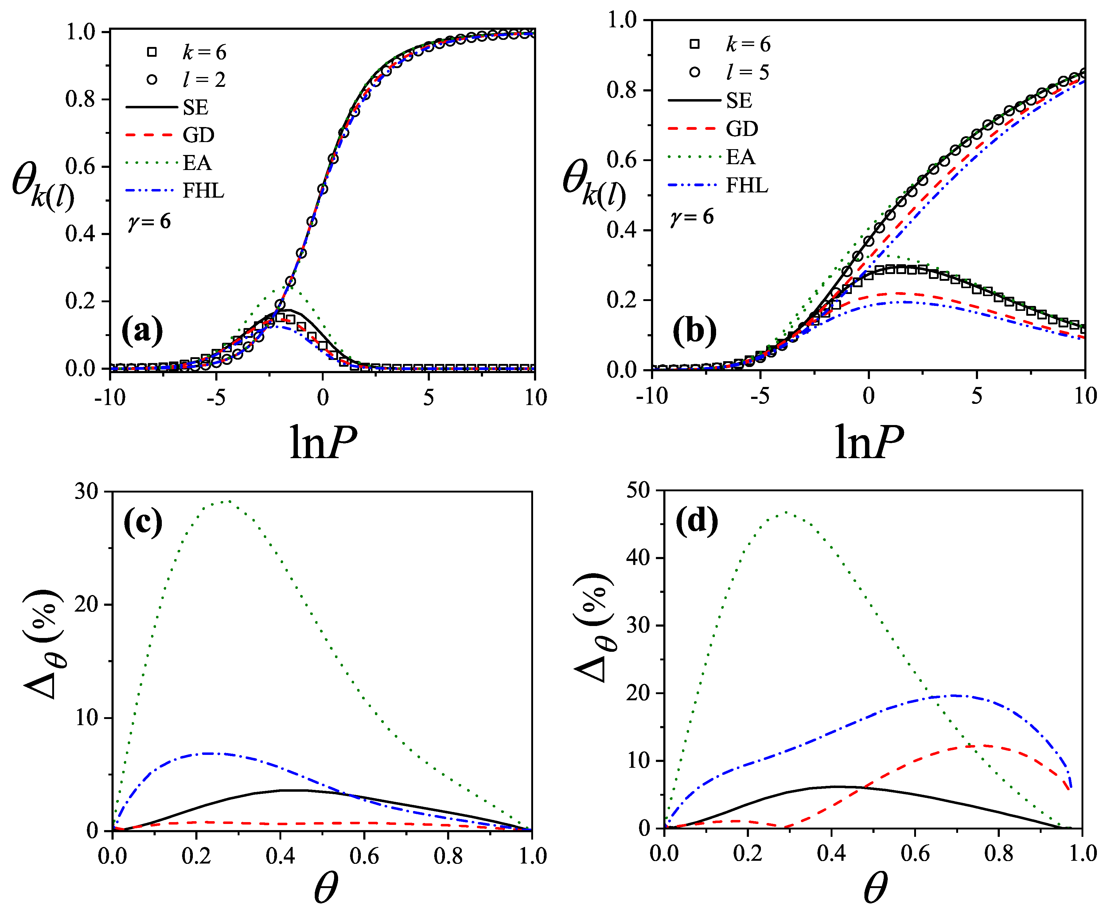
Figure 34.
Average error for fixed k and different values of l: (a) square lattice, and (b) triangular lattice, . The meaning of the lines is indicated in the figure.
Figure 34.
Average error for fixed k and different values of l: (a) square lattice, and (b) triangular lattice, . The meaning of the lines is indicated in the figure.
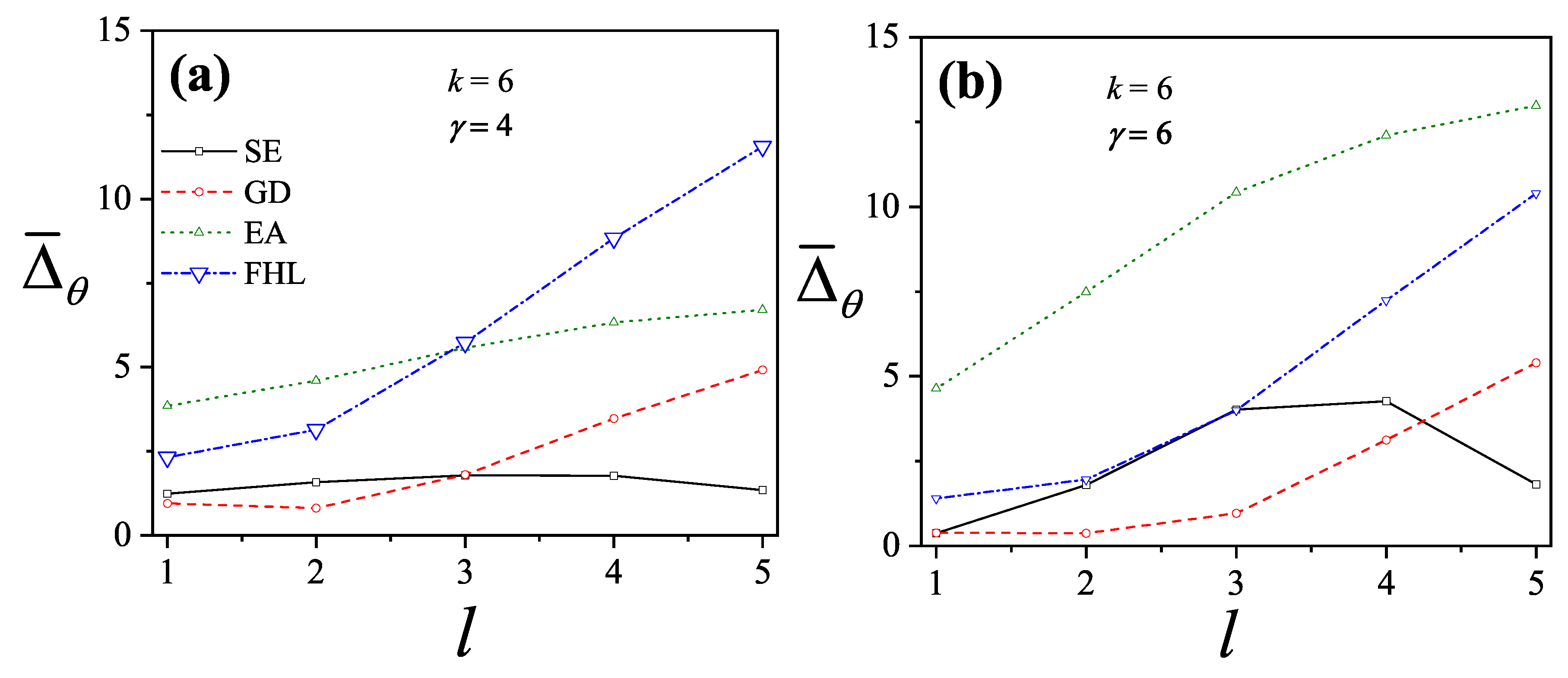
Figure 35.
Comparison between experimental and theoretical adsorption isotherms for a binary mixture: (a) CH4/C2H6 and (b) C2H6/C3H6 adsorbed on a commercial activated carbon. Symbols represent experimental data from Ref. [116] and lines correspond to results from Equation (193). The parameters used in the fitting procedure are listed in Table 1.
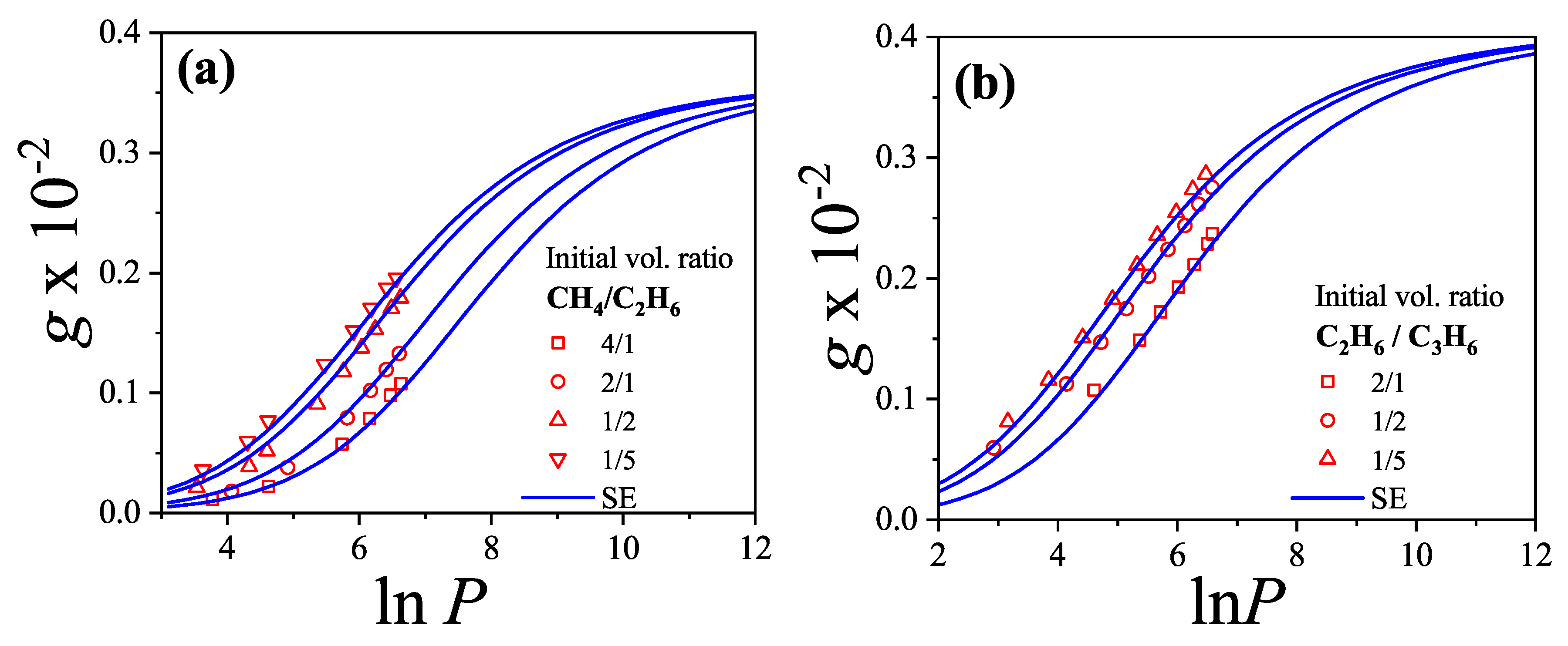
Figure 36.
Adsorption isotherms for homonuclear dimers adsorbed on a honeycomb lattice with nearest-neighbor interactions. Symbols, solid lines and dashed lines represent results from Monte Carlo simulations, and , respectively. The dotted lines are included in the figure as a guide for the eyes. a) Attractive case: full circles, ; open circles, ; open squares, ; open up triangles, ; open diamonds, and open down triangles, . b) Repulsive case: full circles, ; full hexagons, ; full squares, ; full up triangles, ; full diamonds, ; full down triangles, and full stars, . Inset: Adsorption isotherms from for and different values of k as indicated.
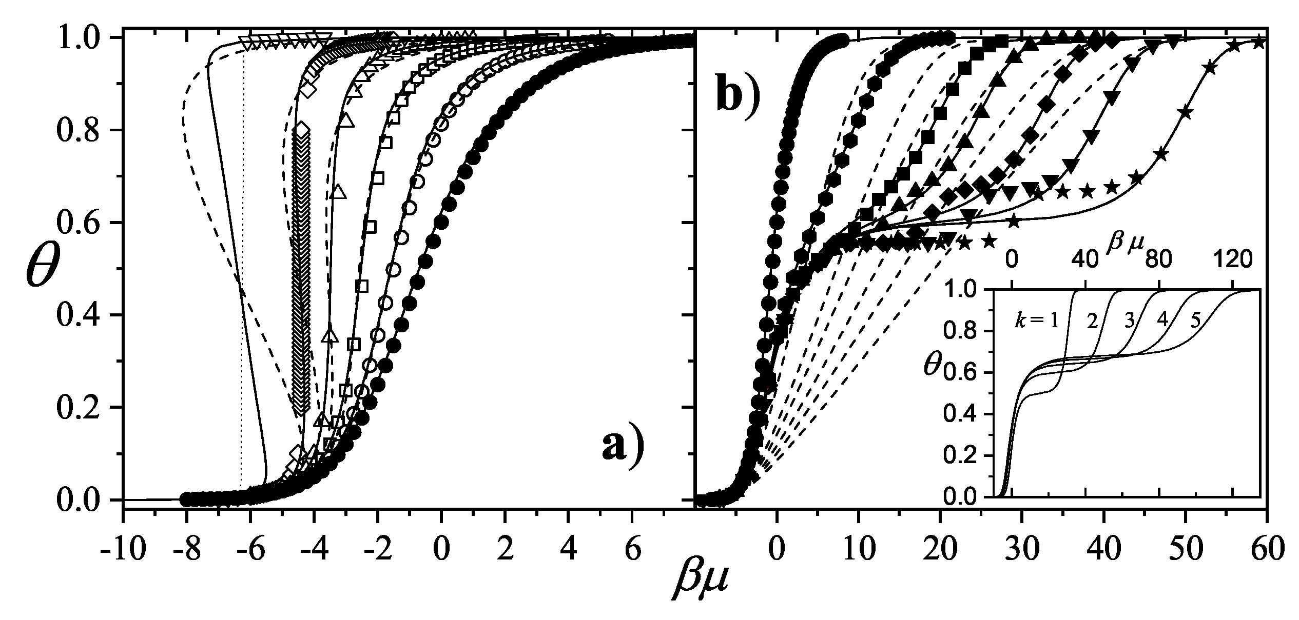
Figure 37.
Adsorption isotherms for homonuclear dimers adsorbed on a square lattice with nearest-neighbor interactions. Symbols, solid lines and dashed lines represent results from Monte Carlo simulations, and , respectively. The dotted lines are included in the figure as a guide for the eyes. a) Attractive case: full circles, ; open squares, ; open up triangles, ; open diamonds, and open down triangles, . b) Repulsive case: full circles, ; full squares, ; full up triangles, ; full diamonds, and full down triangles, . Inset: Adsorption isotherms from for and different values of k as indicated.

Figure 38.
Adsorption isotherms for homonuclear dimers adsorbed on a triangular lattice with nearest-neighbor interactions. Symbols, solid lines and dashed lines represent results from Monte Carlo simulations, and , respectively. The dotted lines are included in the figure as a guide for the eyes. a) Attractive case: full circles, ; open circles, ; open squares, ; open diamonds, and open up triangles, . b) Repulsive case: full circles, ; full squares, ; full up triangles, ; full diamonds, and full down triangles, . Inset: Adsorption isotherms from for and different values of k as indicated.
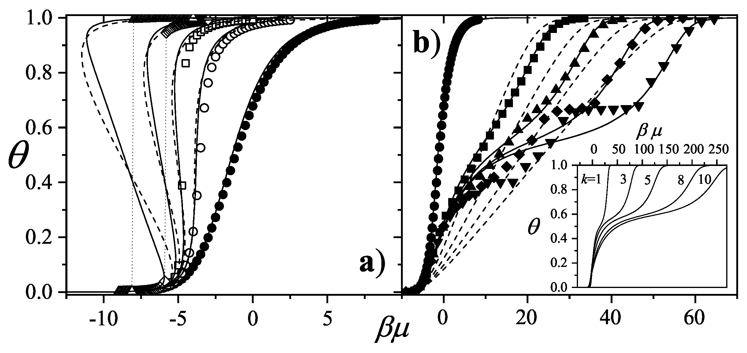
Figure 39.
Snapshots of the ordered phases corresponding to repulsive dimers adsorbed on a honeycomb lattice. a) Low-coverage ordered structure (LCOP); b) high-coverage ordered structure (HCOP) and c) LCOP-HCOP mixture according to the predictions of QCA.
Figure 39.
Snapshots of the ordered phases corresponding to repulsive dimers adsorbed on a honeycomb lattice. a) Low-coverage ordered structure (LCOP); b) high-coverage ordered structure (HCOP) and c) LCOP-HCOP mixture according to the predictions of QCA.
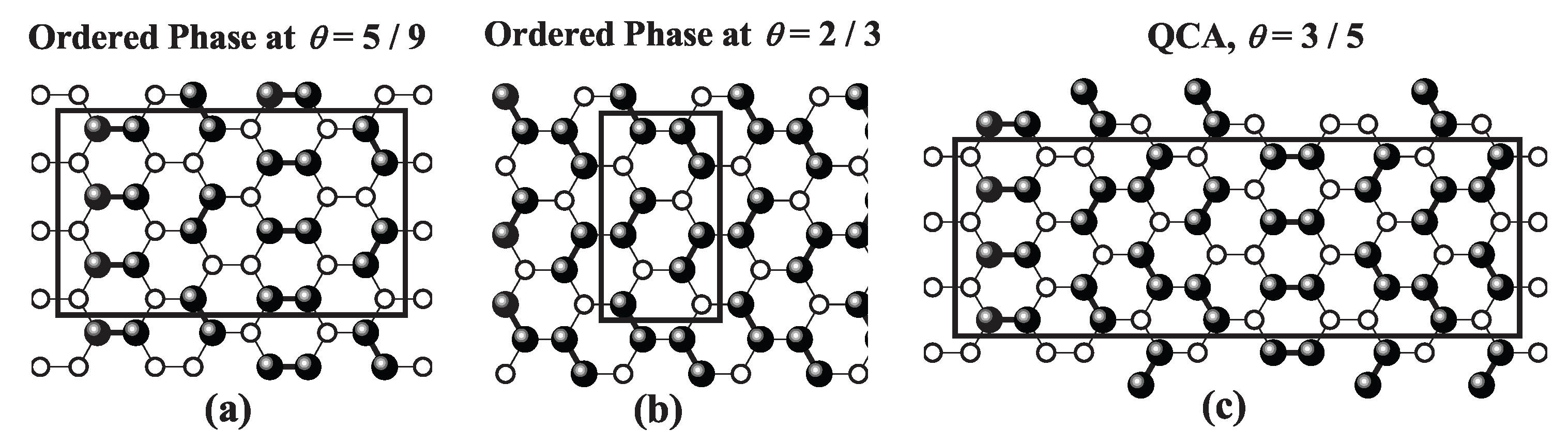
Figure 40.
As Figure 39 for square lattices.
Figure 40.
As Figure 39 for square lattices.
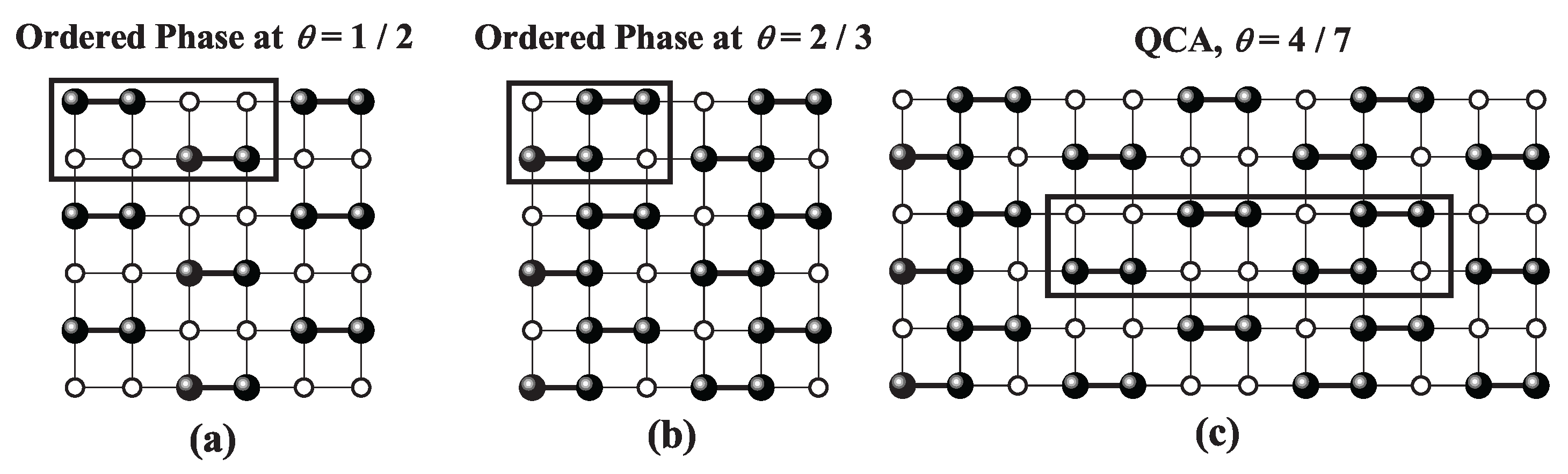
Figure 41.
As Figure 39 for triangular lattices.
Figure 41.
As Figure 39 for triangular lattices.
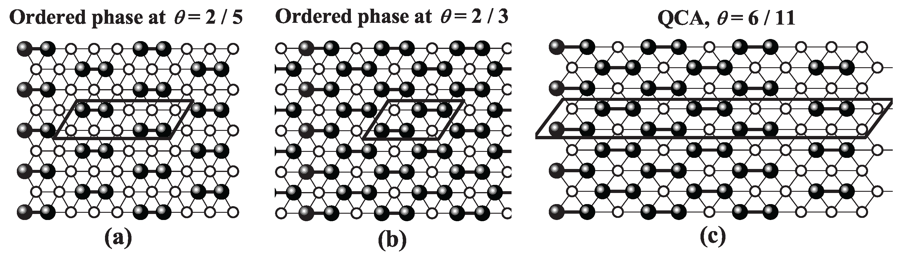
Figure 42.
Absolute error , versus surface coverage for adsorption isotherms of dimers. The symbology is as follows: a) Squares, ; triangles, and circles, . b) Squares, ; triangles, and circles, . Full and open symbols correspond to comparisons with and , respectively.
Figure 42.
Absolute error , versus surface coverage for adsorption isotherms of dimers. The symbology is as follows: a) Squares, ; triangles, and circles, . b) Squares, ; triangles, and circles, . Full and open symbols correspond to comparisons with and , respectively.
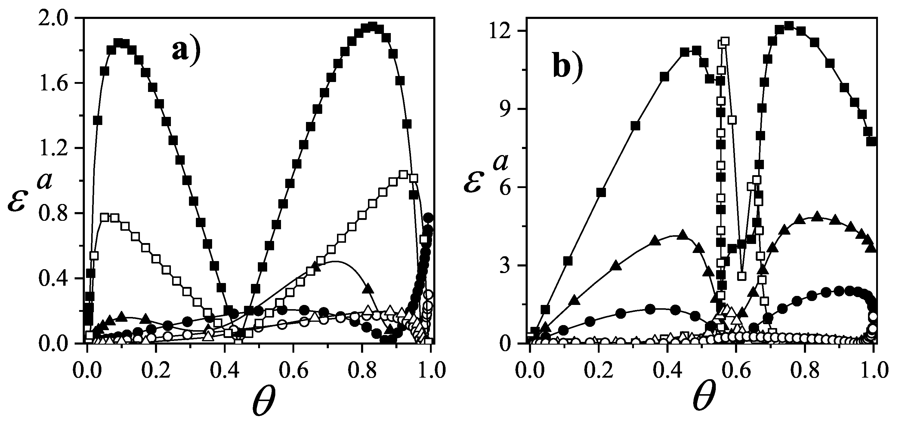
Figure 43.
Integral error , versus lateral interaction (in units) for different geometries as indicated.
Figure 43.
Integral error , versus lateral interaction (in units) for different geometries as indicated.
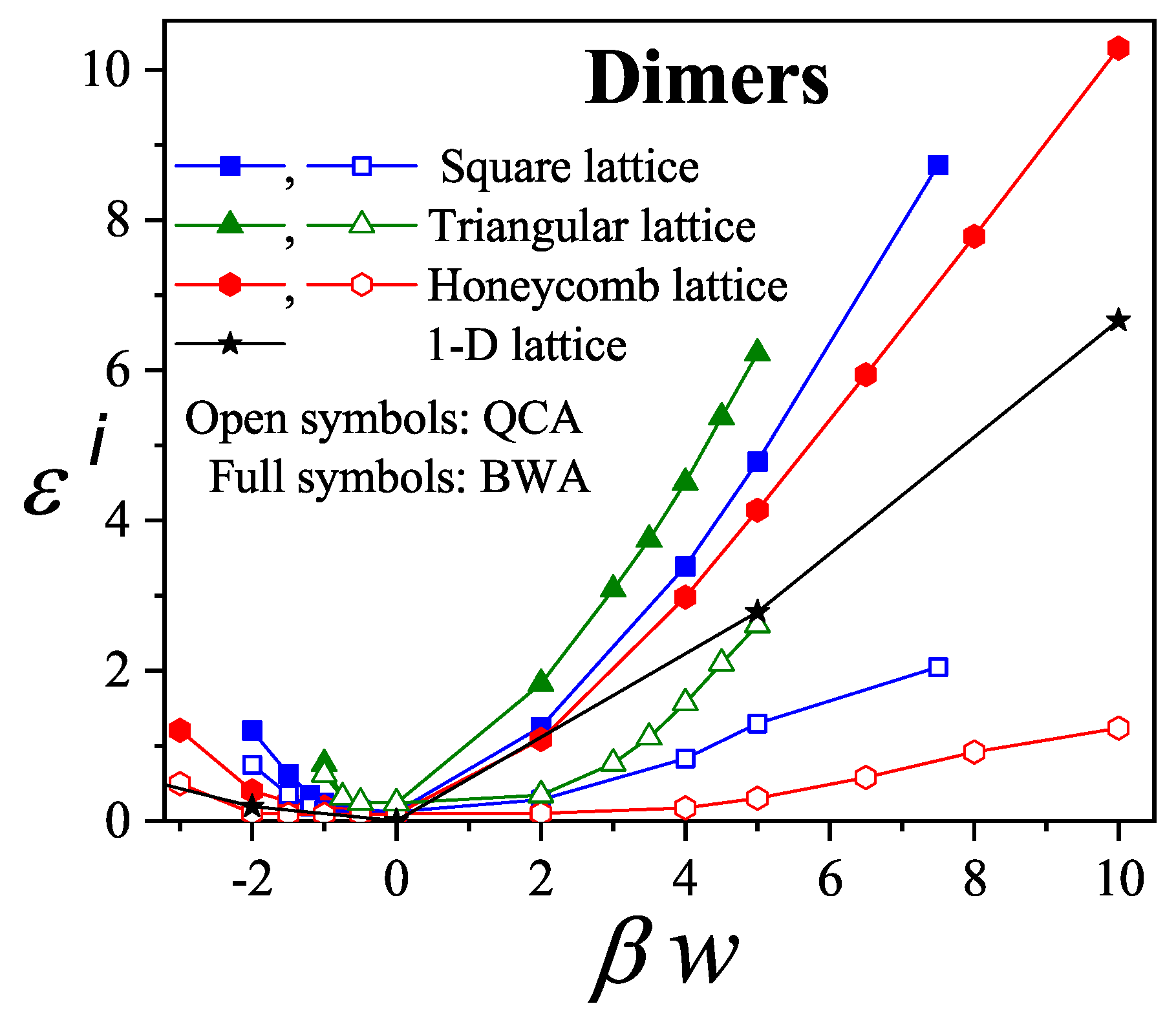
Figure 44.
Adsorption isotherms for adsorbed in zeolite fitted by . Symbols correspond to data from Ref. [120] and lines represent theoretical results from Equation (336).
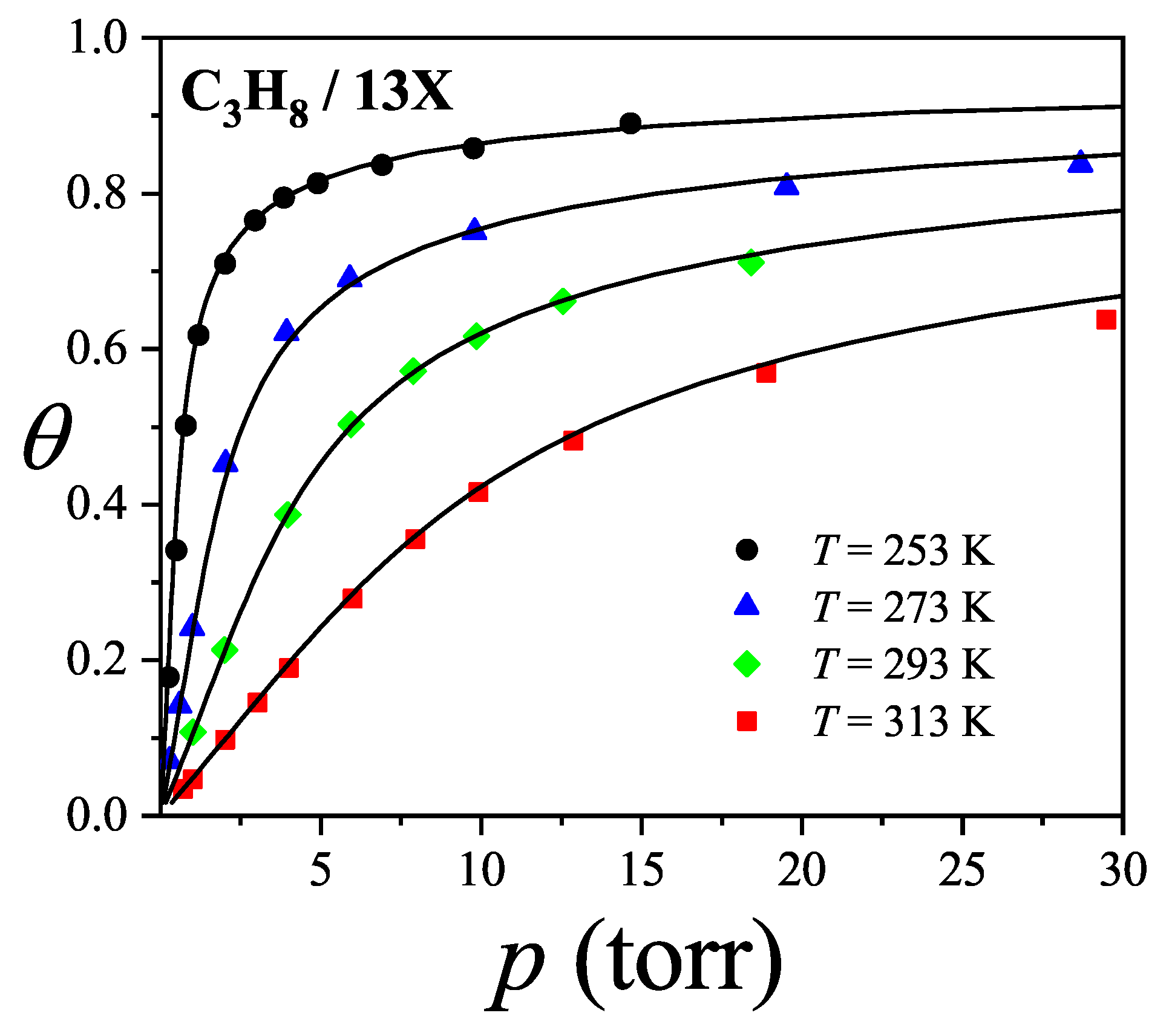
Figure 45.
Derivative of the adsorbed amount versus pressure () for the same set of data plotted in Figure 44.
Figure 45.
Derivative of the adsorbed amount versus pressure () for the same set of data plotted in Figure 44.
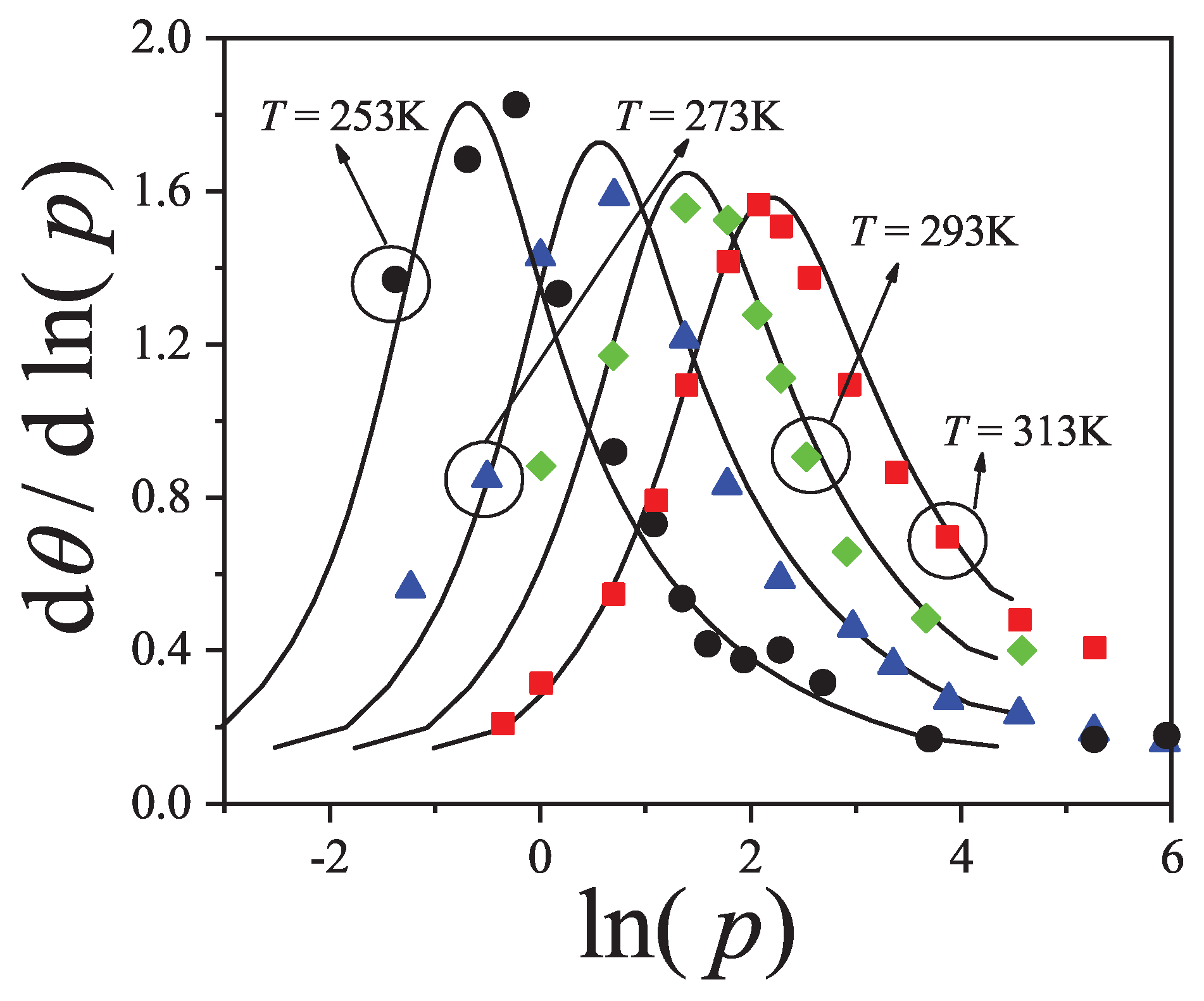
Figure 47.
Temperature dependence of equilibrium constant, , arising from fitting. Squares, red circles and black circle correspond to fitting from Refs. [120,121,122], respectively. reported in Table 2 is the absolute value of the slope of the solid line.
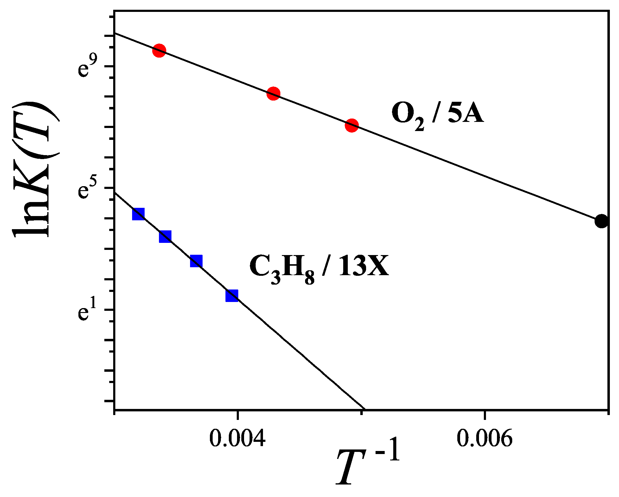
Figure 48.
Comparison between Monte Carlo simulations of dimers, trimers and tetramers adsorbed on square lattices and theoretical isotherm from [Equation (125)]. g values from best fitting are indicated in the figure for each case. Inset: Configurational entropy versus coverage for dimers adsorbed on square lattices. Symbols represent simulation data and lines provide theoretical results for different values of g as indicated in the text.
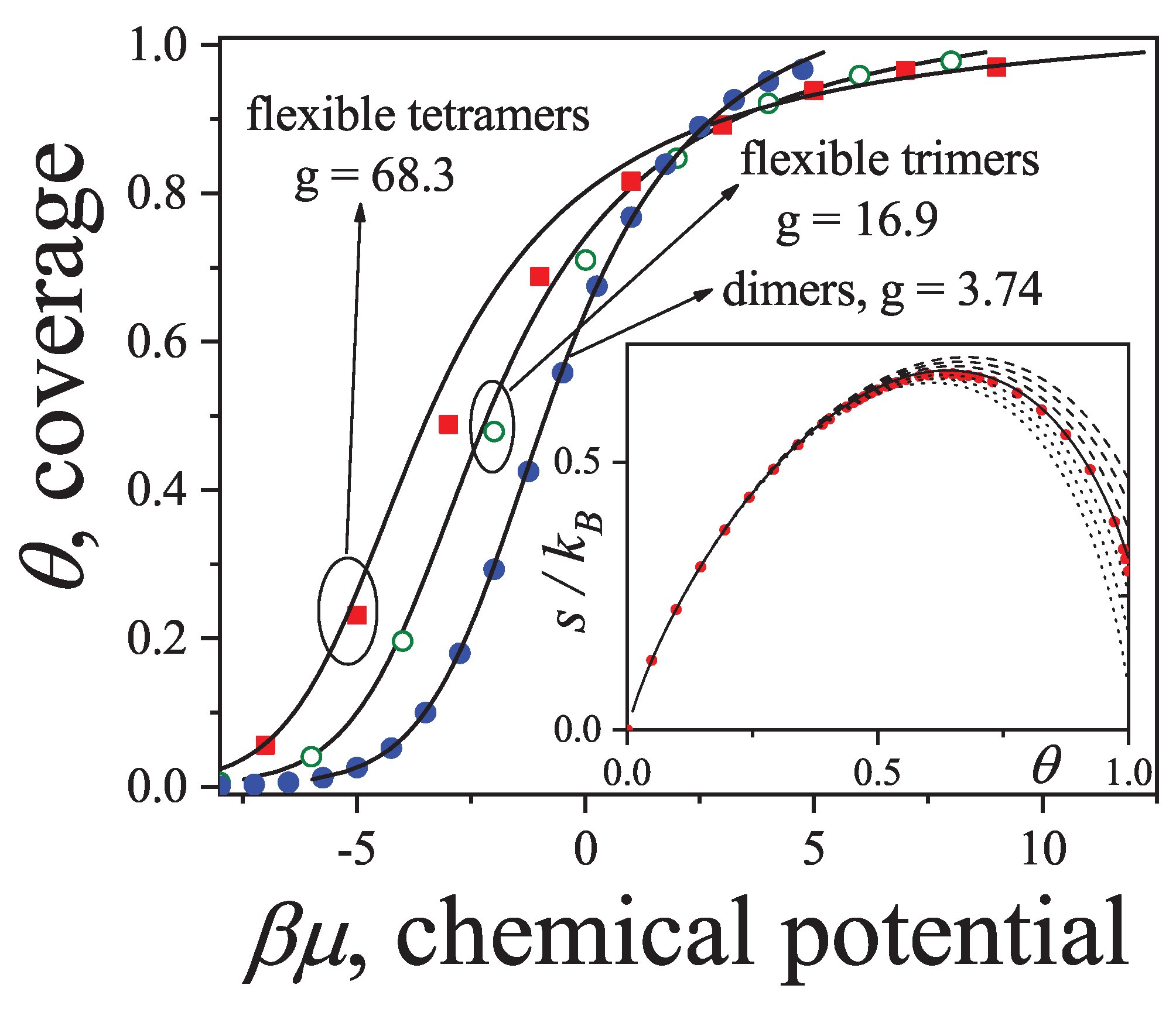
Figure 49.
Partial adsorption isotherms for an equimolar monomer()-monomer() mixture on an one-dimensional lattice. Parameter values (figure): and . Parameter values (inset): , , and .
Figure 49.
Partial adsorption isotherms for an equimolar monomer()-monomer() mixture on an one-dimensional lattice. Parameter values (figure): and . Parameter values (inset): , , and .
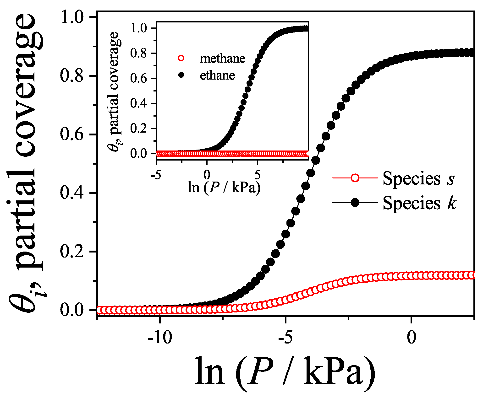
Figure 50.
Partial adsorption isotherms for an equimolar methane()-ethane() mixture on an one-dimensional lattice. Parameter values: , , and .
Figure 50.
Partial adsorption isotherms for an equimolar methane()-ethane() mixture on an one-dimensional lattice. Parameter values: , , and .
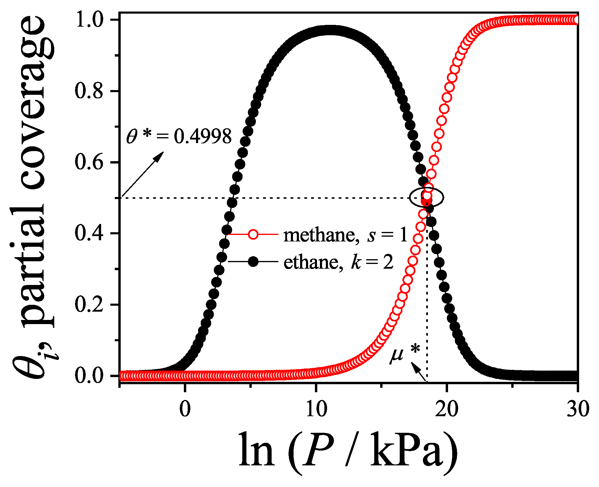
Figure 51.
The adsorption isotherm for methane on single-walled carbon nanotubes is shown, with the coverage (expressed in cm3 Torr/g) plotted on the Y-axis against the relative pressure on the X-axis. Initially, there is a steep rise in coverage at low pressures, followed by a region where the coverage increases linearly with pressure. The point at which the isotherm first diverges from this linear behavior (indicated by the arrow aligned with the X-axis in the figure) is identified as point B. This point is interpreted as corresponding to the completion of the monolayer.
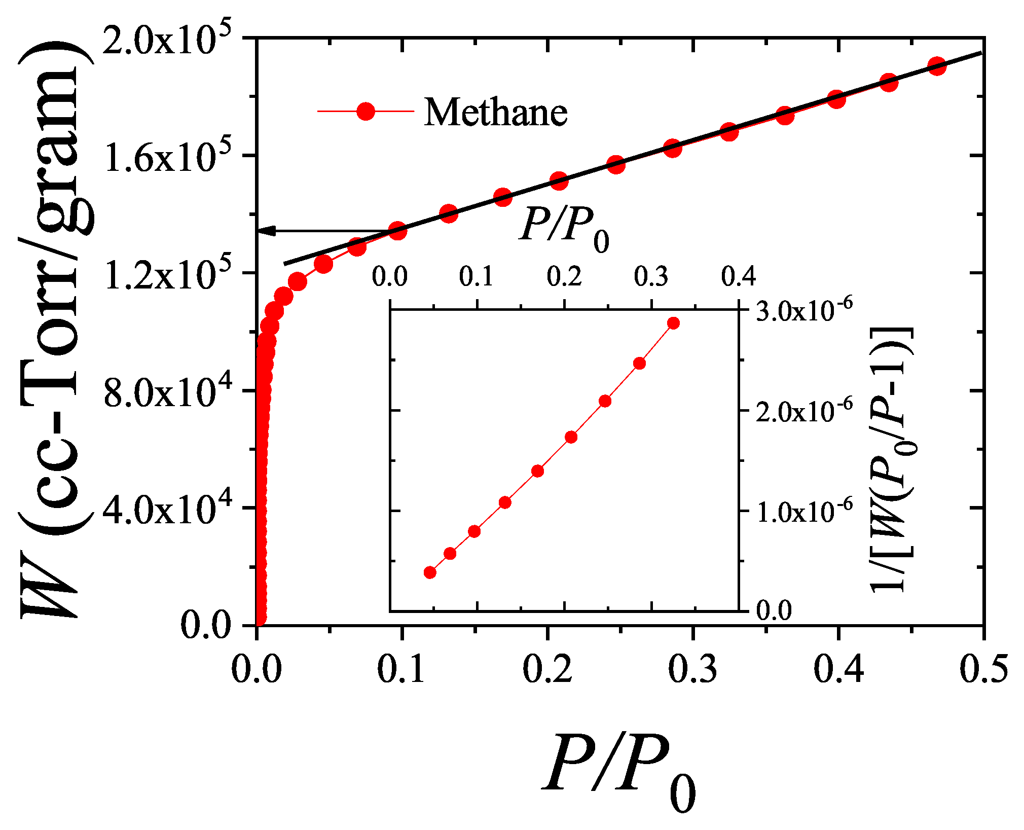
Figure 52.
Adsorption isotherms for methane (77.3K), ethane (165 K), propane (190 K), and butane (220 K) adsorption on single-walled carbon nanotubes. The coverage in cm3 Torr/g (Y axis) is presented as a function of relative pressure (X axis).
Figure 52.
Adsorption isotherms for methane (77.3K), ethane (165 K), propane (190 K), and butane (220 K) adsorption on single-walled carbon nanotubes. The coverage in cm3 Torr/g (Y axis) is presented as a function of relative pressure (X axis).
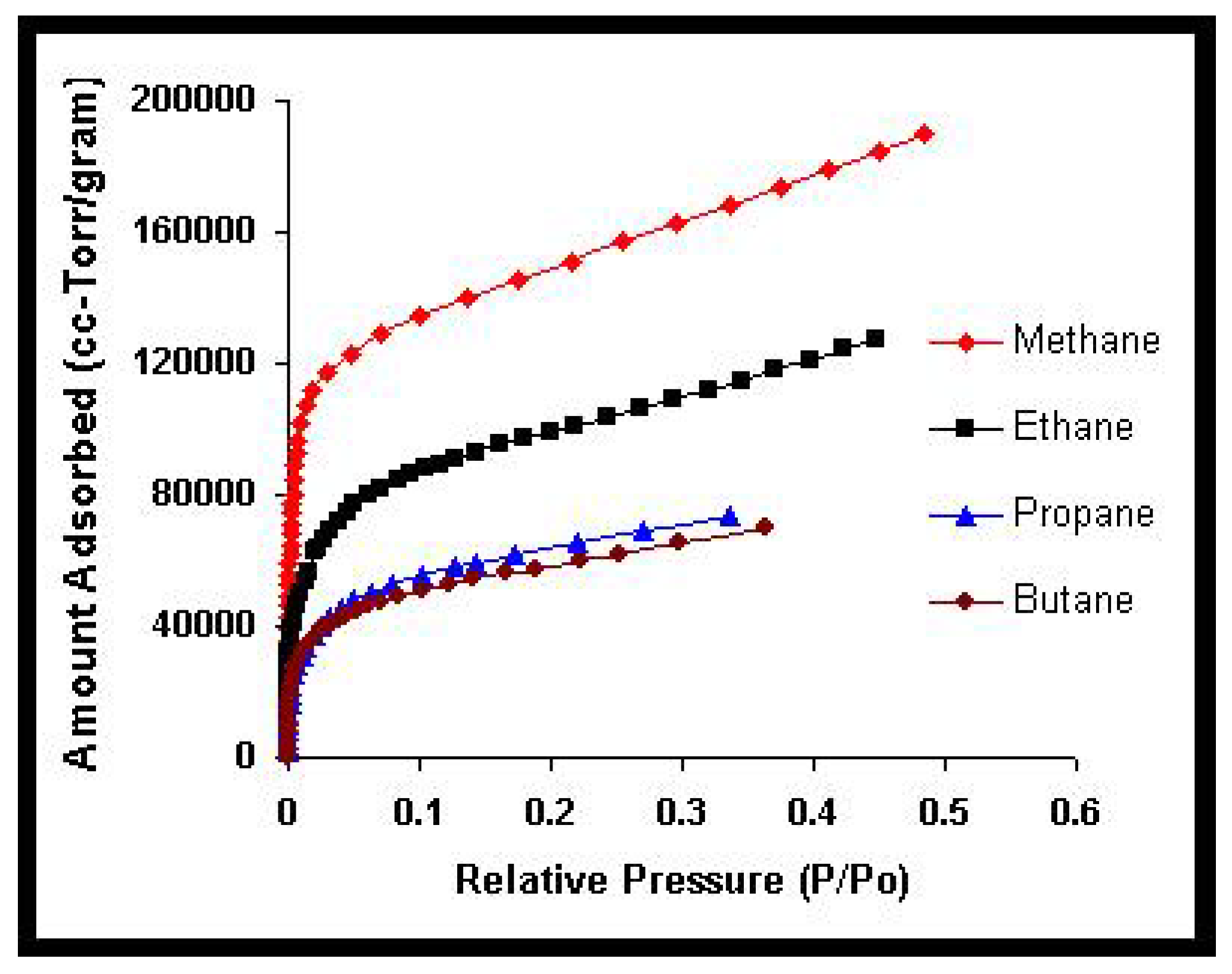
Figure 53.
BET analysis for the adsorption isotherms for methane, ethane, propane, and butane on single-walled carbon nanotubes shown in Figure 52.
Figure 53.
BET analysis for the adsorption isotherms for methane, ethane, propane, and butane on single-walled carbon nanotubes shown in Figure 52.
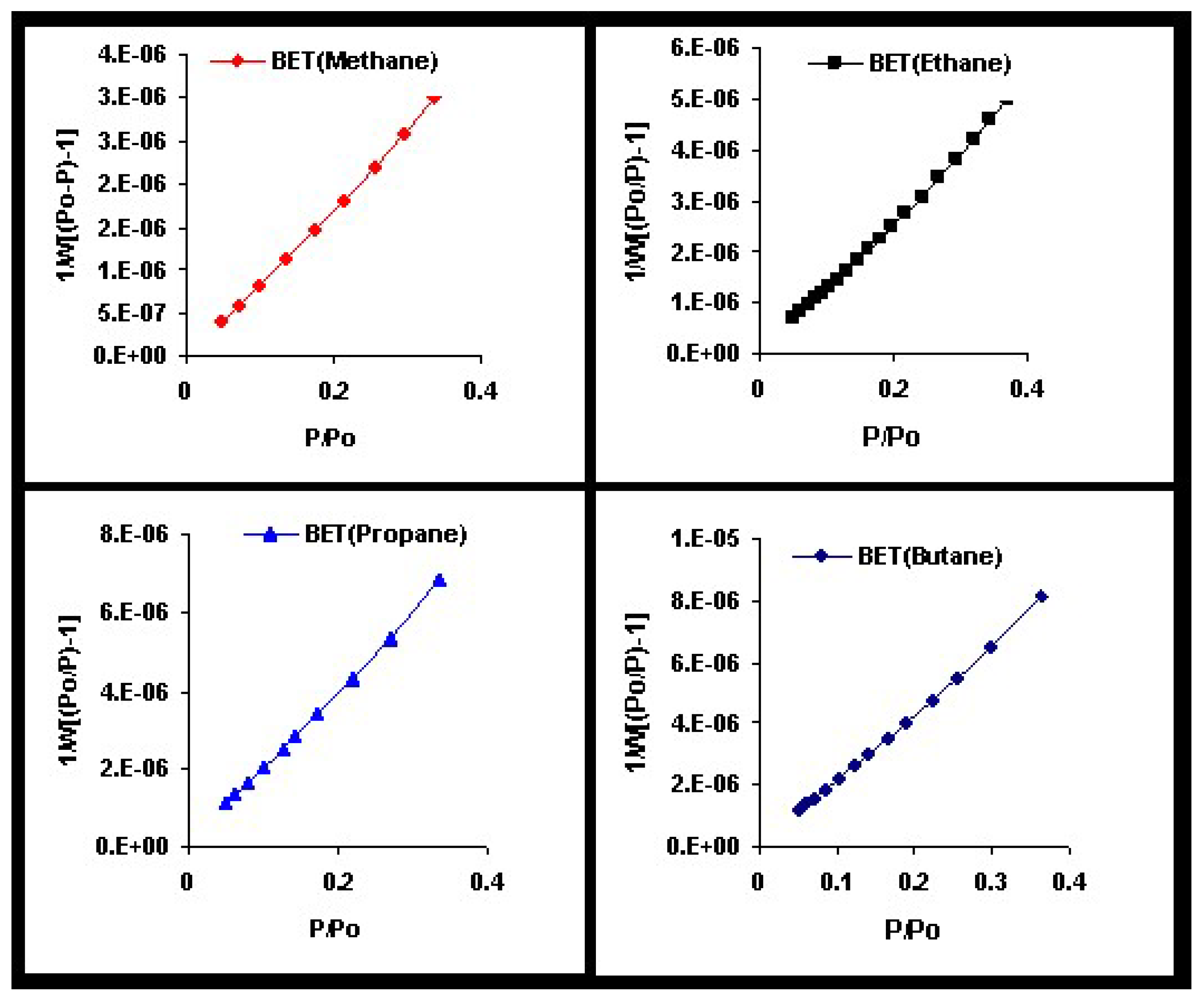
Figure 54.
Specific surface area of single-walled carbon nanotubes computed using the BET and the point B methods. The specific surface area in m2/g (Y axis) is presented as a function of number of carbon atoms in the adsorbate (X axis).
Figure 54.
Specific surface area of single-walled carbon nanotubes computed using the BET and the point B methods. The specific surface area in m2/g (Y axis) is presented as a function of number of carbon atoms in the adsorbate (X axis).
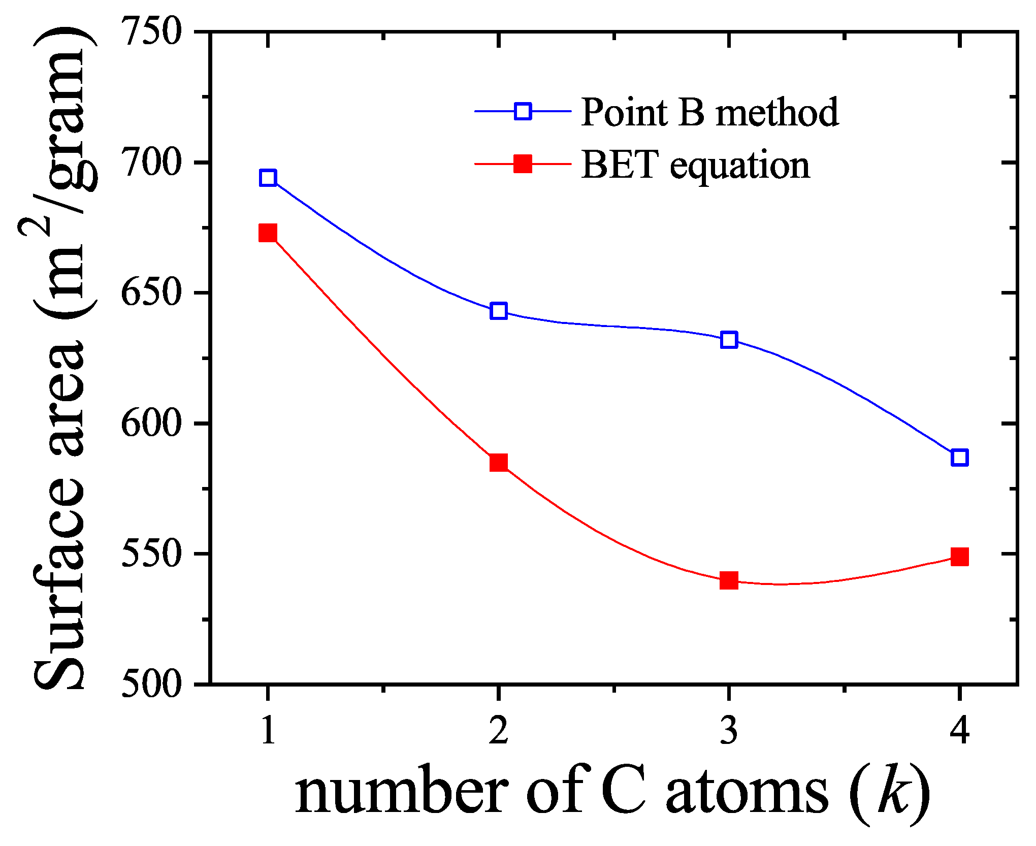
Figure 55.
Fit of the low-pressure region of the butane isotherm data to Equation (343) in the text (obtained in the MBET approach). The value of the monolayer capacity is extracted from this fit.
Figure 55.
Fit of the low-pressure region of the butane isotherm data to Equation (343) in the text (obtained in the MBET approach). The value of the monolayer capacity is extracted from this fit.
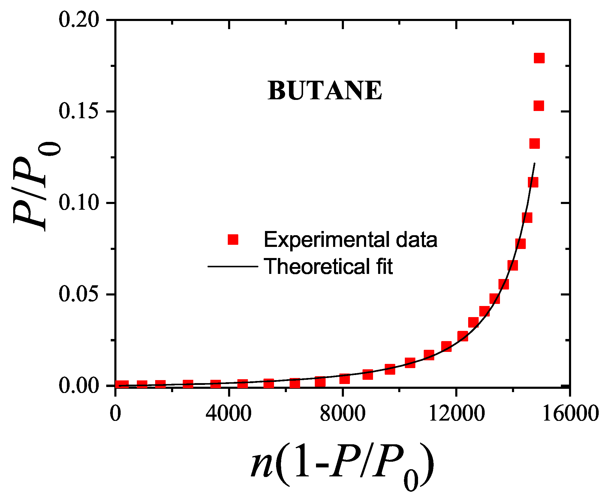
Figure 56.
Specific surface area values for single-walled carbon nanotubes were calculated using four different methods: BET, point B, procedure A, and procedure B. The results, expressed in m2/g (Y-axis), are plotted as a function of the number of carbon atoms in the adsorbate molecules (X-axis). To maintain clarity in the figure, error bars are shown only for the values obtained using procedure B.
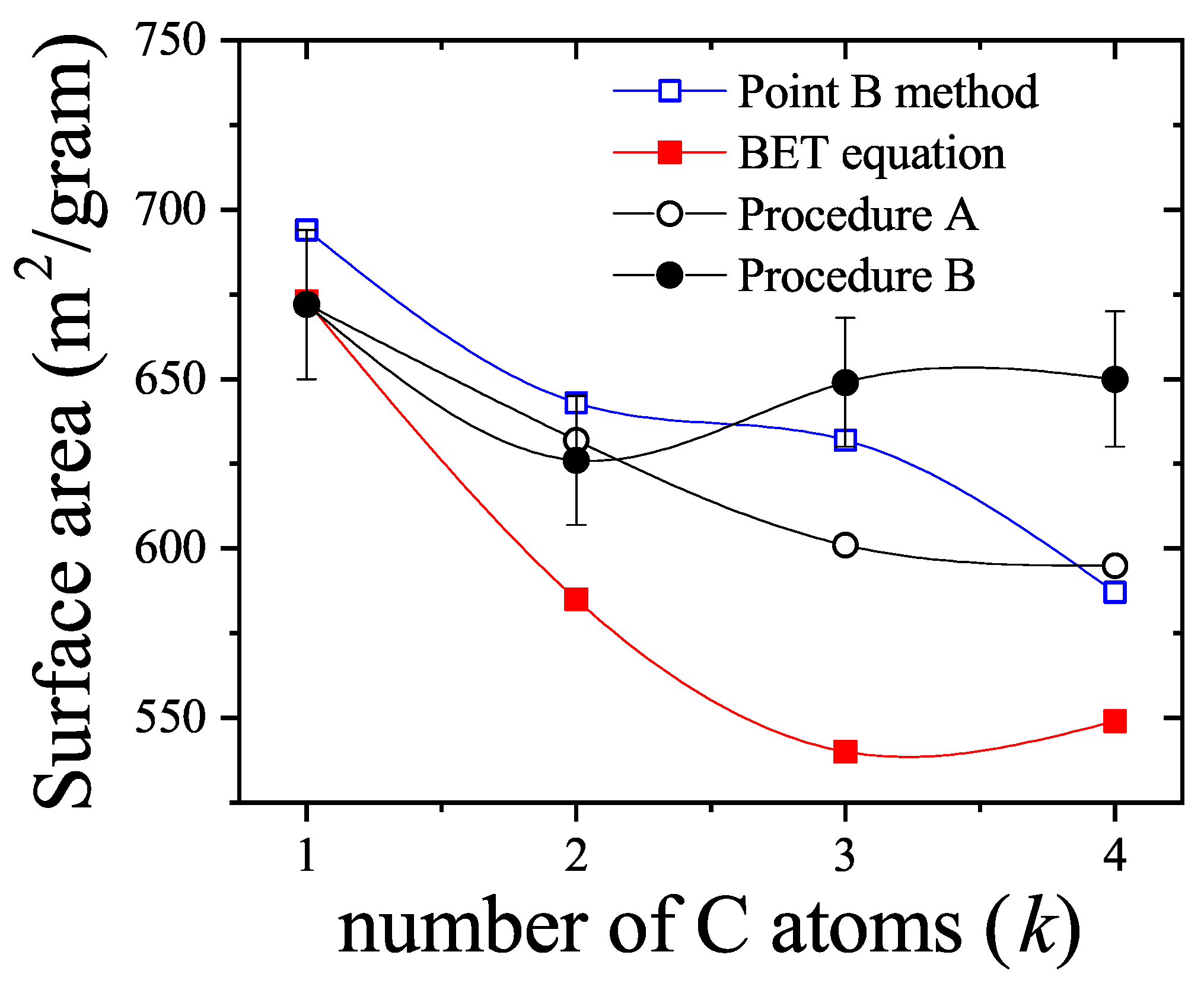
Figure 57.
Relative step velocity as a function of the concentration for monomers [, red line, Equation (355)] and tetramers [, blue line, Equation (358)]. In the two cases, .
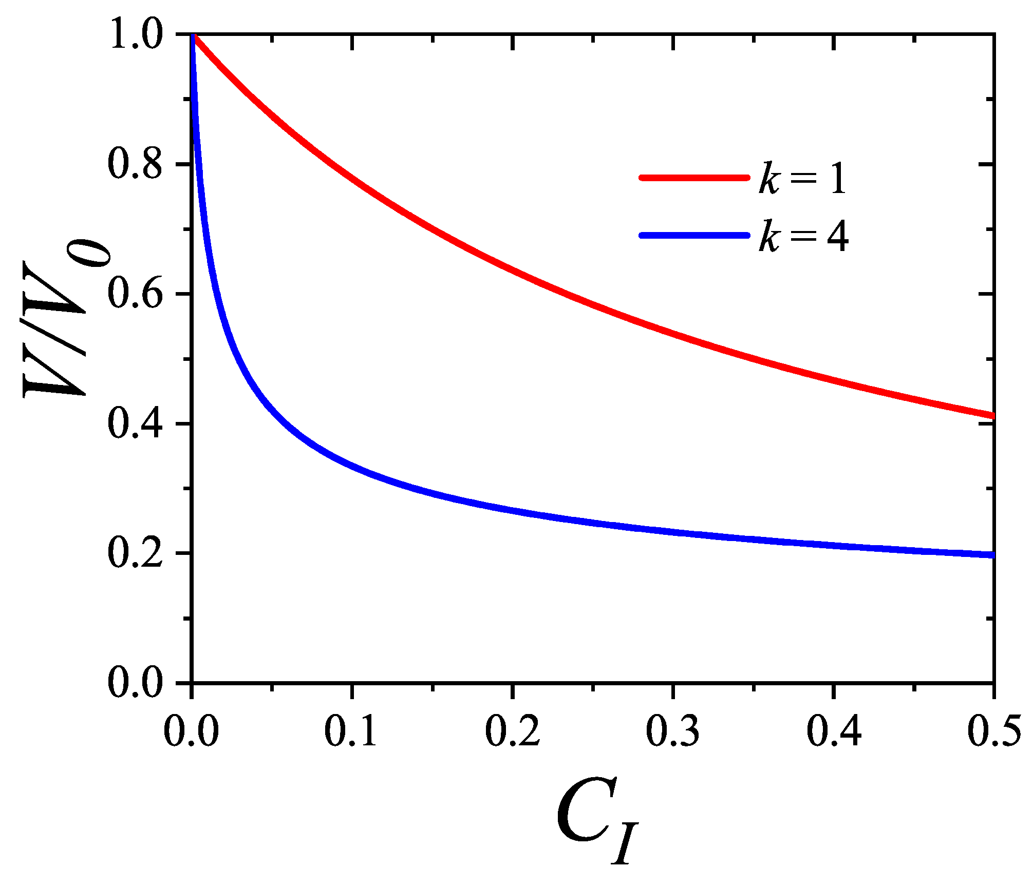
Figure 58.
Relative growth rates of the faces of KBr crystals as a function of impurity concentration. Aliphatic carboxylic acids, HCOOH, CH3COOH, C2H5COOH and C3H7COOH were used as impurities. Symbols correspond to experimental data [171], solid lines represent results from Equations (355–358) and dashed lines correspond to KM model [168]. The parameters used in the theoretical models are listed in Table 4.
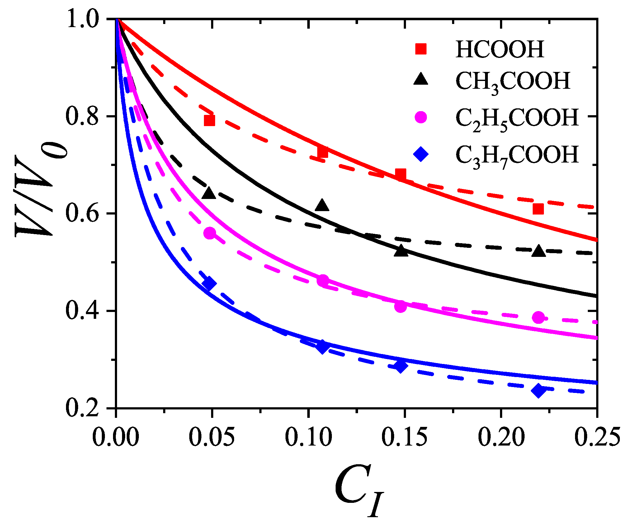
Figure 59.
Order parameter for , , (dotted); , (dashed); , (solid); , , (dash-dotted). Critical densities for the nematic transition are very approximately, , , , , respectively. All cases correspond to densities of states functions , [ consequently, also the entropy surface ] restricted to vanish at the saturation line in the plane .
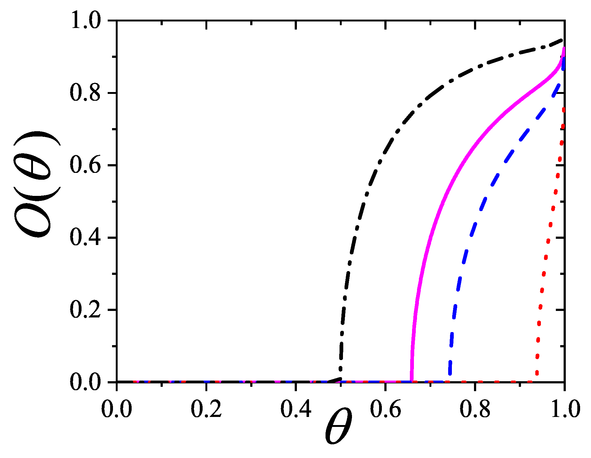
Figure 60.
Order parameter versus for (solid), ; (dashed), ; (short-dashed), ; (dotted), . Parameters of the empirical high density entropy term form Equations (??)-(??), , , . The superimposed full symbols for and correspond to the analytical results from the density of states function Equation (373) of the statistics for: , and , .
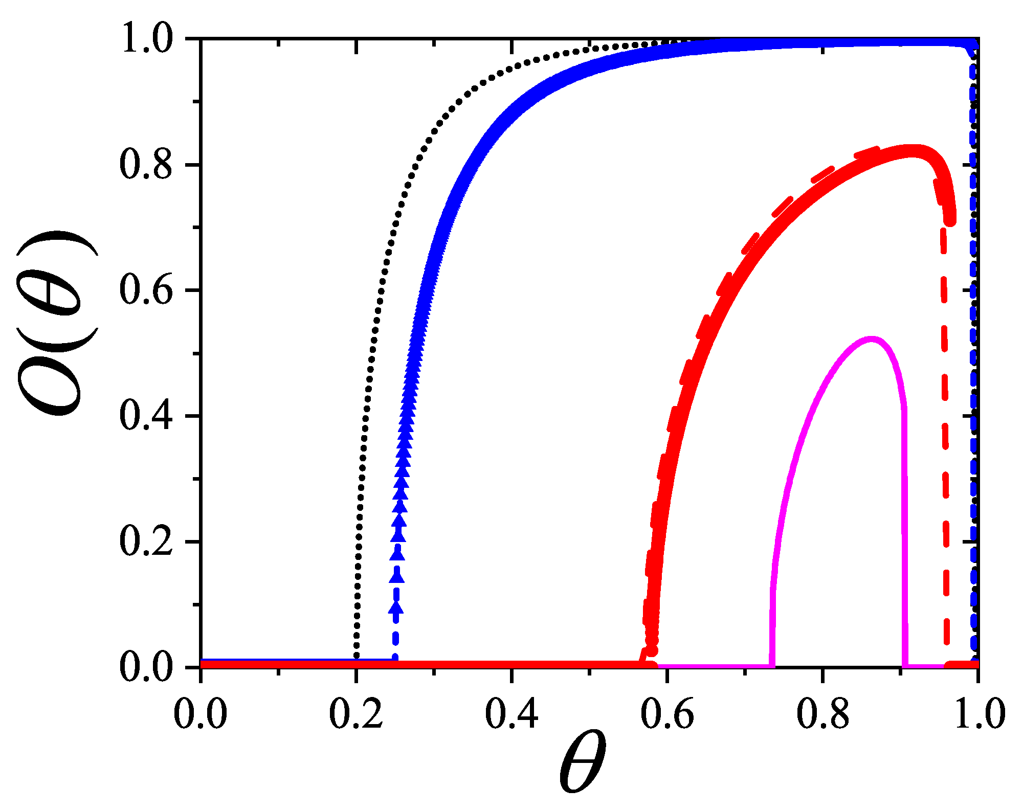
Figure 61.
Full Helmholtz free energy surface for as a function of the state occupation numbers and along the two lattice directions. Black dots represent the equilibrium states. Branches represents the high and low density phases of the nematic transition.
Figure 61.
Full Helmholtz free energy surface for as a function of the state occupation numbers and along the two lattice directions. Black dots represent the equilibrium states. Branches represents the high and low density phases of the nematic transition.
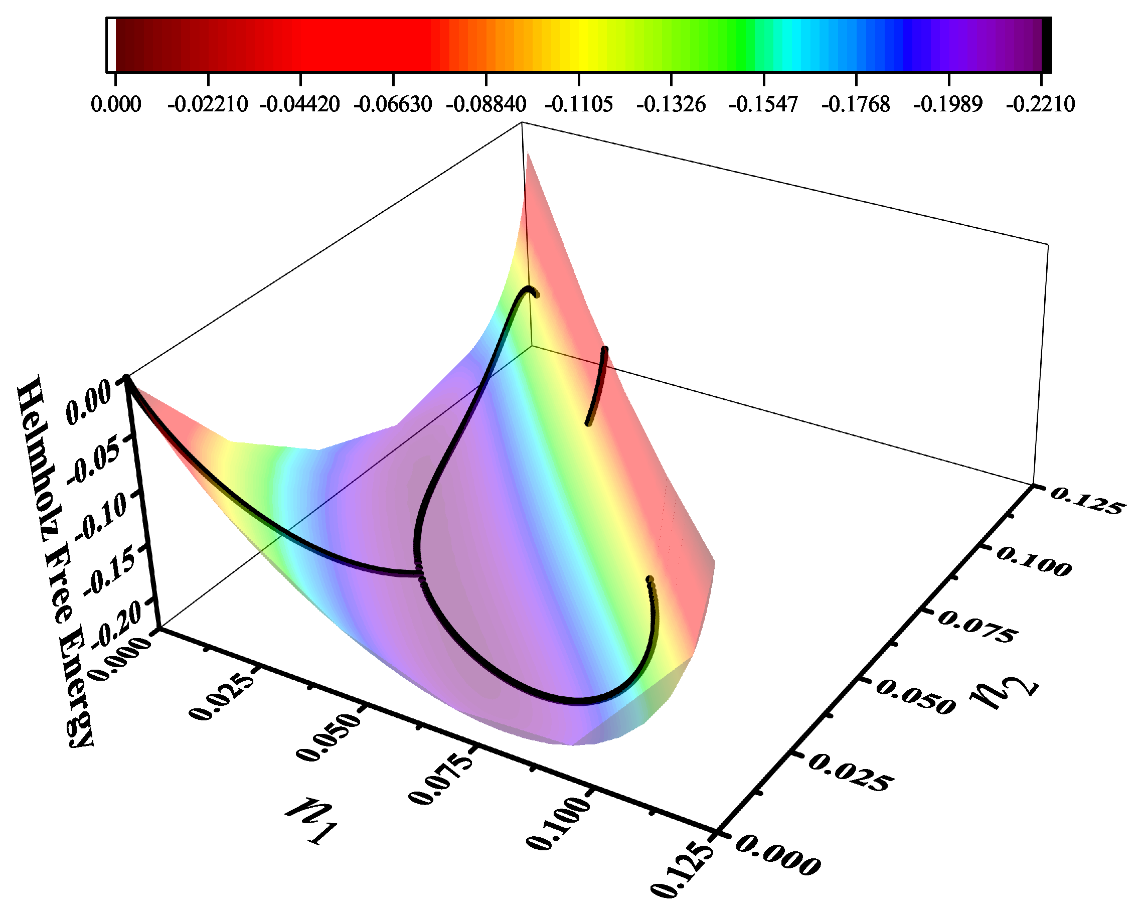
Figure 62.
Lattice coverage versus for . Red and blue lines are theoretical results from the formalism with the generalized density of states Equation (373). The high-density (upper blue) and low-density (lower blue) branches, along with the total coverage (red), are shown. The inset highlights the first-order transition at high coverage. Green lines (overlapping) correspond to the empirical entropy correction. Symbols are MC simulation data. Parameters: , , , , , , , , .
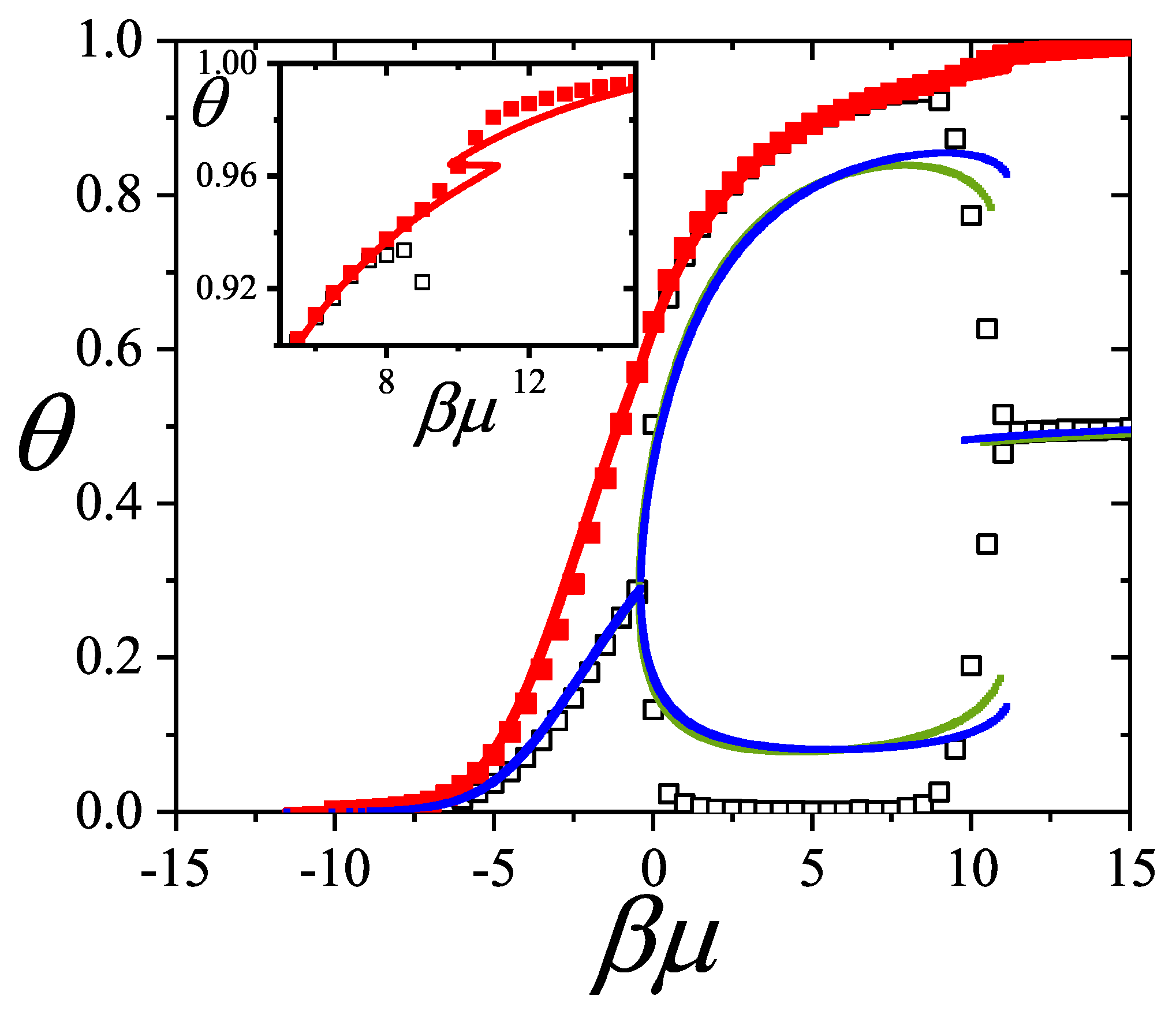
Figure 63.
Same as Figure 62 but for . Parameters: , , , , , , , , .
Figure 63.
Same as Figure 62 but for . Parameters: , , , , , , , , .
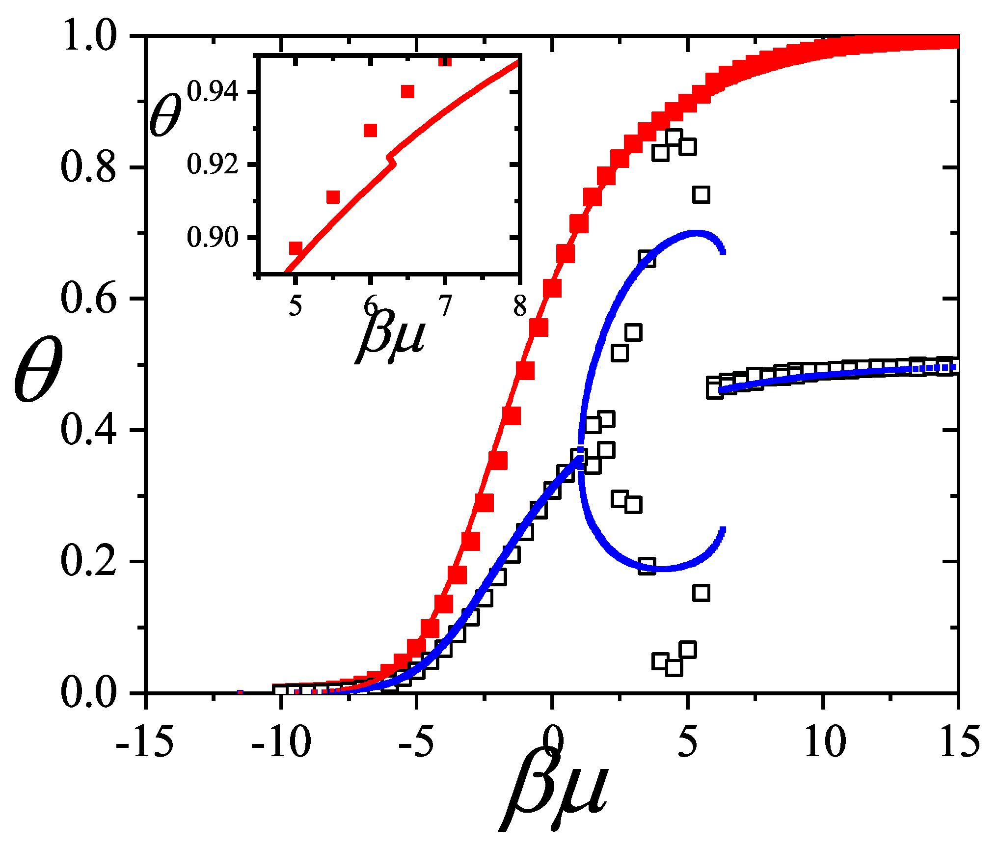
Figure 64.
Coverage vs. for (main figure) and (inset). Lines are theoretical statistics results with generalized density of states Equation (373). MC data are shown as symbols.
Figure 64.
Coverage vs. for (main figure) and (inset). Lines are theoretical statistics results with generalized density of states Equation (373). MC data are shown as symbols.
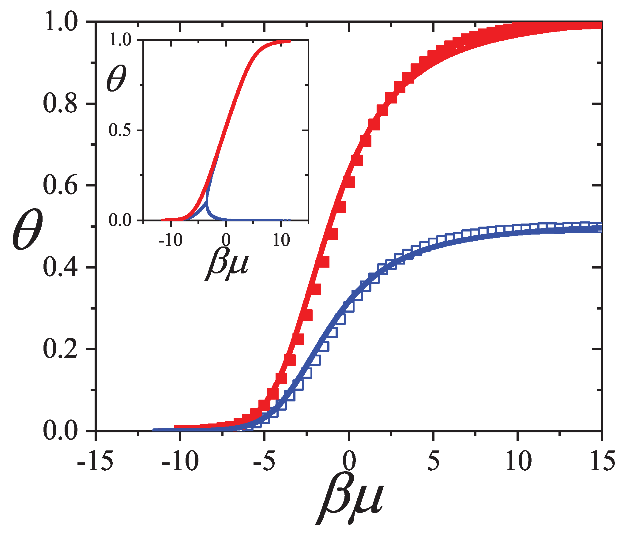
Figure 67.
Example of a system of tetramers on a square lattice. (a) Current state. (b) Horizontal tetramers removed. (c) Detail of row j with three segments (only segments with are showed).
Figure 67.
Example of a system of tetramers on a square lattice. (a) Current state. (b) Horizontal tetramers removed. (c) Detail of row j with three segments (only segments with are showed).
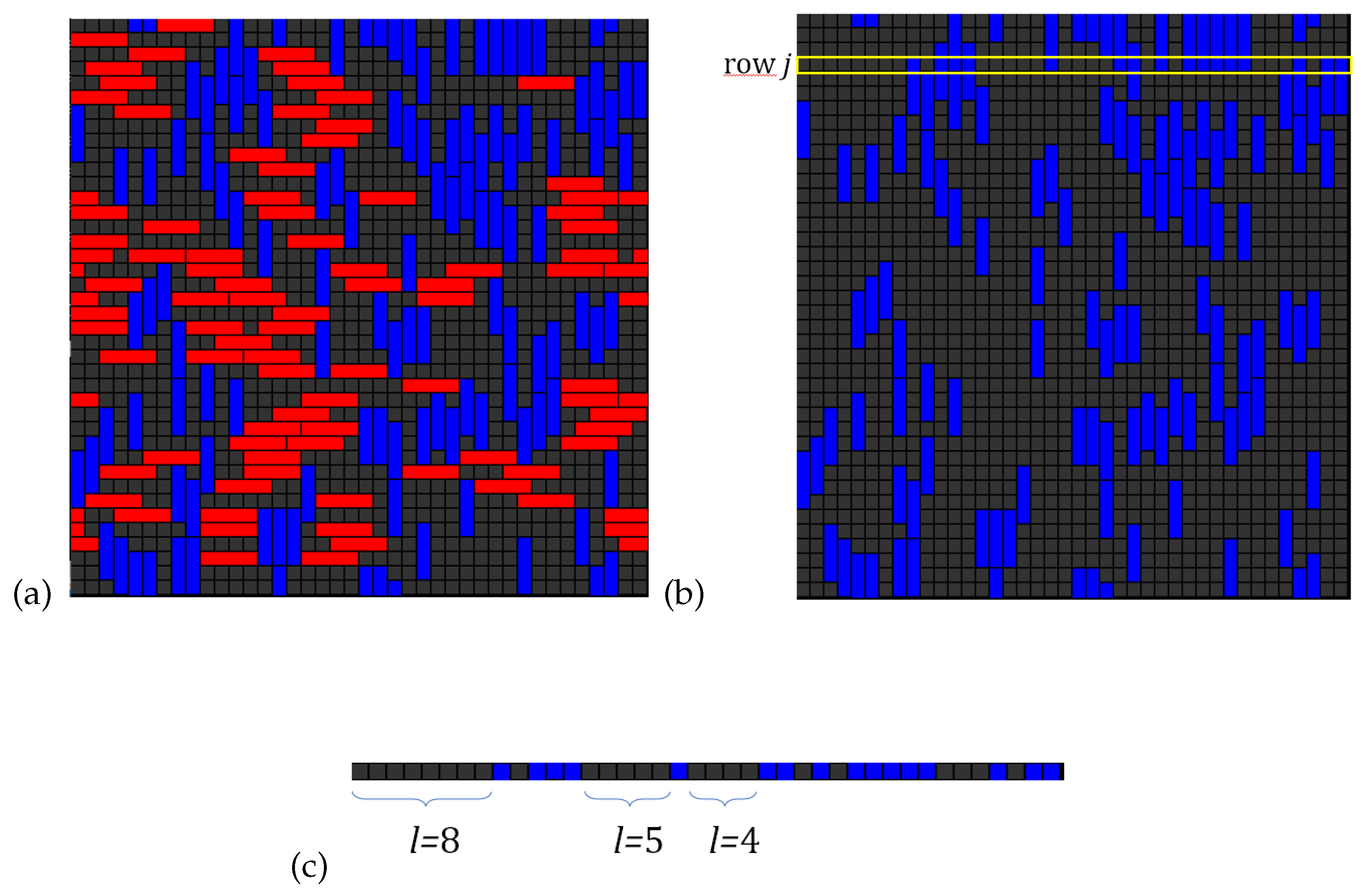
Figure 68.
Refilling process of a segment by tetramers. Each branch is made with precalculated probabilities of the 1D case that depend on T and . Red represents a deposited k-mer and grey represents a deposited empty site.
Figure 68.
Refilling process of a segment by tetramers. Each branch is made with precalculated probabilities of the 1D case that depend on T and . Red represents a deposited k-mer and grey represents a deposited empty site.
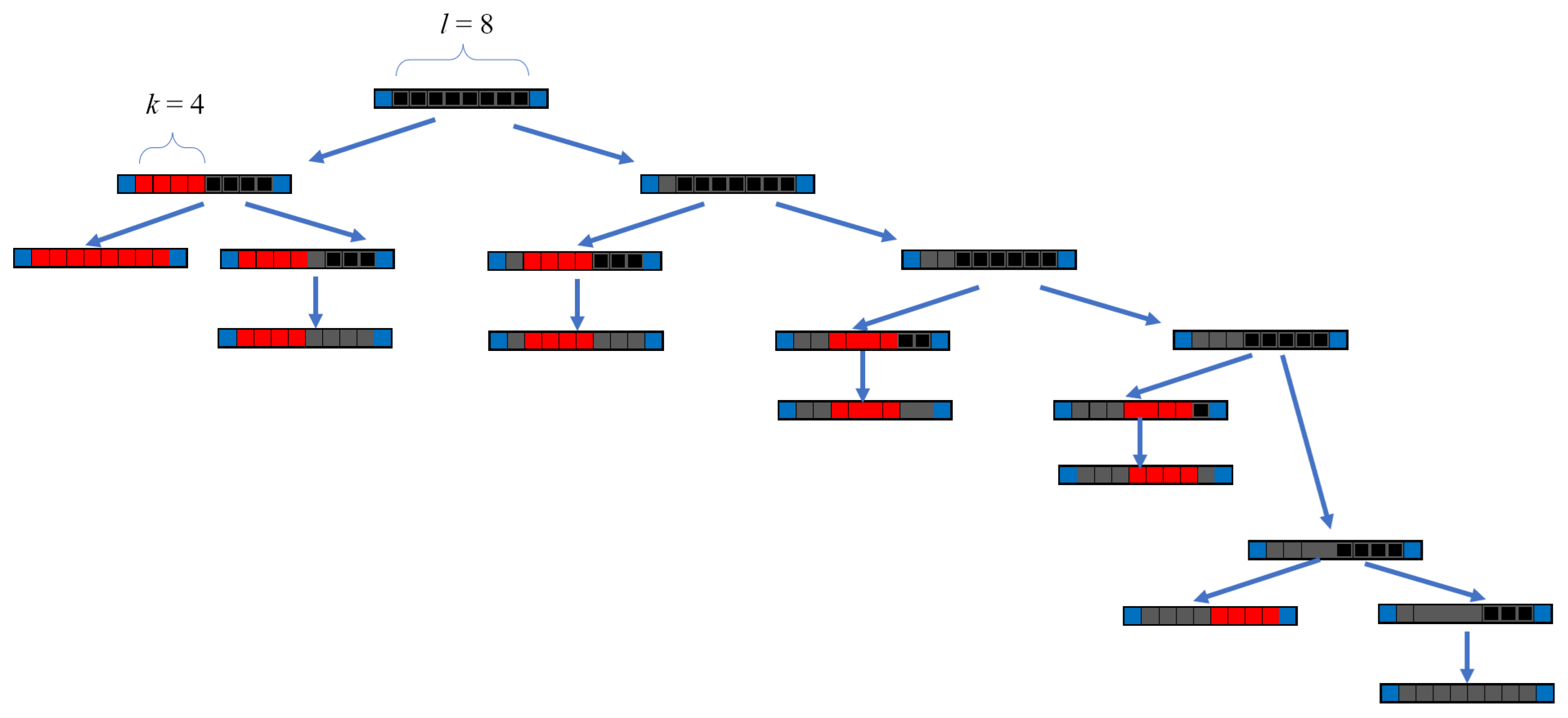
Figure 69.
Dimers () adsorbed on a square lattice of sites. Typical units are labeled. This represents the system of interest (original).
Figure 69.
Dimers () adsorbed on a square lattice of sites. Typical units are labeled. This represents the system of interest (original).
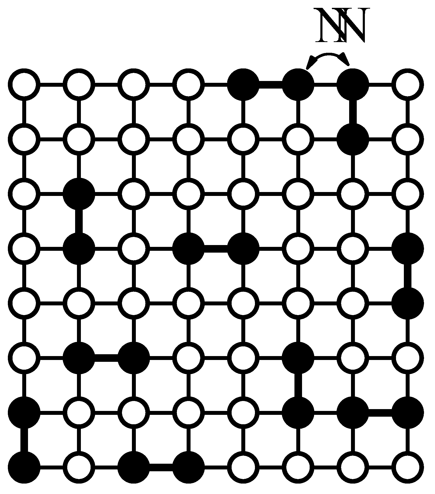
Figure 70.
a) Square lattice of sites representing the lattice of the artificial system; strong and weak sites are symbolized by circles and squares respectively. b) Configuration of dimers in the lowest energy state (ground state) according to the artificial Hamiltonian of Equation (388).
Figure 70.
a) Square lattice of sites representing the lattice of the artificial system; strong and weak sites are symbolized by circles and squares respectively. b) Configuration of dimers in the lowest energy state (ground state) according to the artificial Hamiltonian of Equation (388).
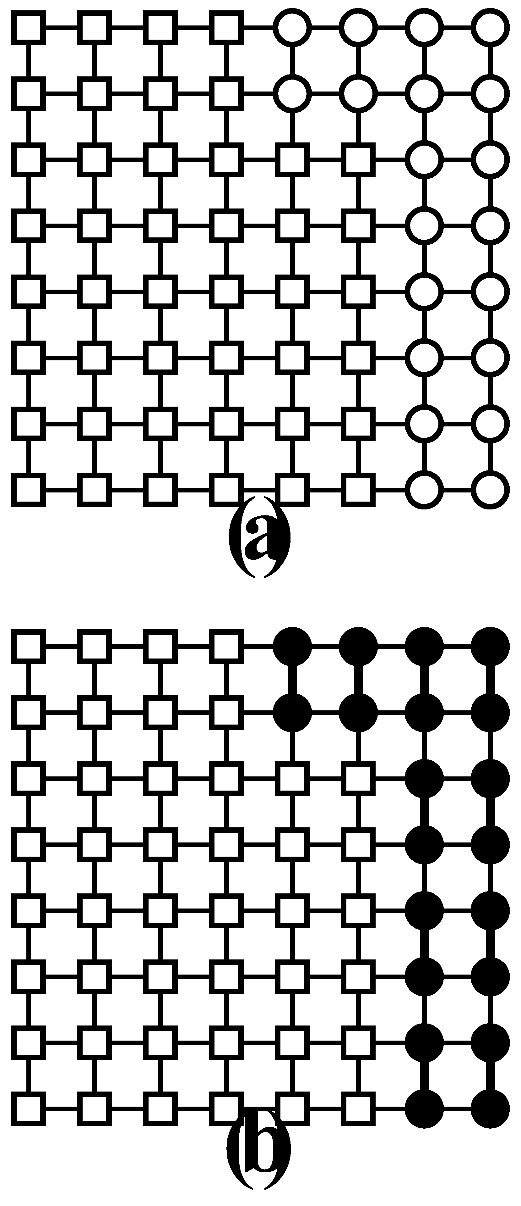
Figure 71.
Mean total energy per site (in units of the interaction energy w) for dimers on a square lattice with nearest-neighbor interaction energy w at fixed coverage . a) Open circles and top x-axis correspond to attractive dimers. b) Full circles and bottom x-axis correspond to repulsive dimers. Simulations were carried out in the canonical ensemble and symbols represent averages over typically MC configurations, after equilibration steps.
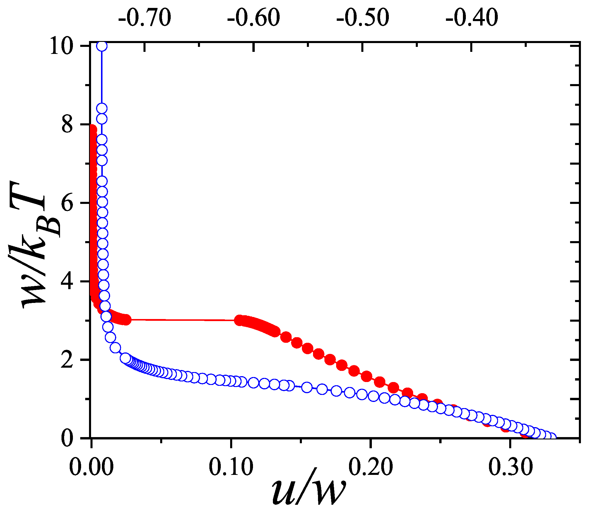

Table 1.
Parameters used in the fitting of Figure 35.
Table 1.
Parameters used in the fitting of Figure 35.
| / | / | |
| (mol. / g) | 0.41 | 0.41 |
| (mmHg−1) | 3.5 | 0.48 |
| (mmHg−1) | 1.6 | 0.6 |
Table 2.
Table of fitting parameters of data in Figure 44 and Figure 46. , , and are expressed in kcal/mol (absolute values given). is expressed in molecules/cavity [(a)] and g. of adsorbent [(b)] for data from Refs. [121] and [122], respectively. (c) and (d) represent experimental values from Refs. [121] and [120], respectively; (e), simulation data from Ref. [123] and (f), interaction energy in the liquid phase [120].
| System | k | m | g | D(%) | |||||
| 2 | 2 | 4 | 3.10 | 0.72 | 5.60 | ||||
| 3 | 1 | 3 | 5.75 | 6.94 | 1.27 | 2.08 |
Table 3.
Single-walled nanotubes samples and gases used in the isotherm measurements.
| sample | type | weight (g) | gas | area/mol on graphite () | isotherm temp (K) |
| SWNTs | HiPco | 0.1727 | methane | 15.4 [145] | 77 |
| SWNTs | HiPco | 0.325 | ethane | 21 [146] | 165 |
| SWNTs | HiPco | 0.325 | propane | 28.8 [147] | 190 |
| SWNTs | HiPco | 0.325 | butane | 32.7 [146] | 220 |
Table 4.
The table shows the parameters used in the theoretical curves of Figure 58.
Disclaimer/Publisher’s Note: The statements, opinions and data contained in all publications are solely those of the individual author(s) and contributor(s) and not of MDPI and/or the editor(s). MDPI and/or the editor(s) disclaim responsibility for any injury to people or property resulting from any ideas, methods, instructions or products referred to in the content. |
© 2025 by the authors. Licensee MDPI, Basel, Switzerland. This article is an open access article distributed under the terms and conditions of the Creative Commons Attribution (CC BY) license (http://creativecommons.org/licenses/by/4.0/).
Copyright: This open access article is published under a Creative Commons CC BY 4.0 license, which permit the free download, distribution, and reuse, provided that the author and preprint are cited in any reuse.


