
Submitted:
03 December 2024
Posted:
06 December 2024
You are already at the latest version
Abstract
This paper explores how competing interactions in the intermolecular potential of fluids affect their structural transitions. The study employs a versatile potential model with a hard core followed by two constant steps, representing wells or shoulders, analyzed in both one-dimensional (1D) and three-dimensional (3D) systems. Comparing these dimensionalities highlights the effect of confinement on structural transitions. Exact results are derived for 1D systems, while the Rational-Function Approximation is used for unconfined 3D fluids. Both scenarios confirm that when the steps are repulsive, the wavelength of the oscillatory decay of the total correlation function evolves with temperature either continuously or discontinuously. In the latter case, a discontinuous oscillation crossover line emerges in the temperature–density plane. For an attractive first step and a repulsive second step, a Fisher–Widom line appears. Although the 1D and 3D results share common features, dimensionality introduces differences: these behaviors occur in distinct temperature ranges, require deeper wells, or become attenuated in 3D. Certain features observed in 1D may vanish in 3D. We conclude that fluids with competing interactions exhibit a rich and intricate pattern of structural transitions, demonstrating the significant influence of dimensionality and interaction features.
Keywords:
competing interactions
; square well
; square shoulder
; discontinuous structural crossover transitions
; Fisher–Widom line
; Rational-Function Approximation
1. Introduction
It is well known that both statistical mechanics and thermodynamics aim at explaining the same phenomena concerning, among other issues, energy, work, and heat exchange in the different systems. While the first approach involves a purely microscopic approximation, the second one is macroscopic in nature. Nevertheless, one of the major purposes of statistical physics is the interpretation and prediction of the macroscopic properties of a system in terms of the interactions between its particles. In the case of liquids, one attempts to understand why and under what circumstances certain phases are stable in well-defined intervals of density and temperature and also to try to relate the thermodynamic, structural, and dynamic properties of those phases with the form and size of the molecules that form the liquid and the nature of the intermolecular interactions [1].
For the description of a multibody system such as a liquid, it is often enough to consider simplified representations which are able to capture the essential elements of real interactions and lead to an adequate description of the observed phenomenology. Therefore, the great attention that has been paid during many decades to interaction potentials consisting of a hard core followed by one or many piecewise constant sections of different widths and heights (which include the square-well and the square-shoulder potentials), is not surprising [2,3,4,5,6,7,8,9,10,11,12,13,14,15,16,17,18,19,20,21,22,23,24,25,26]. With this class of potentials, it has been possible to model and understand many phenomena, such as liquid-liquid transitions [7,8,10], colloidal interactions [11], the density anomaly in water and supercooled liquids [13,14], and the thermodynamic and transport properties of Lennard-Jones fluids [2,3]. In particular, in the case of colloidal dispersions the interaction between a pair of macromolecules is modeled through an effective potential having a short-range attractive part and a long-range repulsive part [27,28,29]. The competition between both parts of this potential leads to interesting phenomenology and induces changes in phase behavior and in the thermodynamic, structural, and transport properties of the system [25,30]. Similarly, in the case of complex fluids, such competing interactions are associated with the aggregation or clustering of surfactants, macromolecules, and colloidal particles in solution, which in turn may produce self-assembly and microphase segregation [31,32,33,34,35,36,37,38,39,40,41,42,43].
Although there is already a vast amount of work concerning the thermodynamic properties of fluids whose molecules interact through potentials in which the attractive and repulsive parts are in competition, the knowledge pertaining to the influence of such competitions on their structural properties is relatively scarce [23].
The decay of the total correlation function, , where is the radial distribution function, serves as a crucial indicator of structural transitions in fluids. These transitions, whether oscillatory or monotonic, reflect changes in the spatial arrangement of particles, driven by the interplay between attractive and repulsive forces in the intermolecular potential. Understanding the decay of has significant implications for phenomena such as crystallization, phase separation, self-assembly, and the mechanical properties of materials.
All of this serves as a motivation for the present paper. In previous work, we have used the so-called Rational-Function Approximation (RFA) approach [44,45] to study various three-dimensional (3D) fluids whose intermolecular potentials consist of a hard-core followed by piecewise constant sections [17,20,22]. This includes not only square-well and square-shoulder fluids but also systems where the intermolecular potential combines square shoulders and square wells.[24]. We have also carried out studies of the asymptotic behavior of the direct and total correlation functions of binary hard-sphere fluid mixtures [46,47,48], which, among other things, exhibit interesting phenomenology concerning structural transitions.
In this paper, we aim to illustrate the effect of competing interactions on structural transitions in fluids. To this end, we consider a fluid of number density and absolute temperature T, where the intermolecular pair potential is given by:
This potential includes a hard core of diameter and two steps characterized by heights and and widths and , respectively. The parameters and are constants satisfying , where denotes the total range of the potential. The sign of each () determines whether the corresponding step is a shoulder () or a well (). This form of the potential is flexible enough to explore various competing interactions. In particular, when or , the potential reduces to either the square-shoulder potential (for ) or the square-well potential (for ), making these cases particular limits of the general model.
This work focuses on examining the qualitative changes in the structural behavior of the system as the potential transitions from the square-shoulder case to more complex potentials, where the second section is always a repulsive barrier ().
If both and are positive, the total correlation function is expected to exhibit oscillatory decay. At very low temperatures, this decay has a wavelength on the order of the range of the repulsive barrier (). Conversely, at very high temperatures, the wavelength aligns with the hard-core diameter (). At a given density, the transition between these behaviors can occur either continuously or discontinuously. In the latter scenario, a discontinuous oscillation crossover (DOC) line would emerge, akin to the one observed in binary hard-sphere mixtures [46,47,49,50,51,52].
On the other hand, if and , one might expect the presence of a Fisher–Widom (FW) line, which separates a region in the T vs plane where the asymptotic decay of is damped oscillatory from a region where the decay is purely exponential and monotonic. For a given , a competition between a DOC line and an FW line could arise as transitions from positive to increasingly negative values.
From this point onward, we adopt the hard-core diameter as the unit of length (), so all distances will be expressed in units of . The reduced density is then given by , where d is the dimensionality of the system. Since we assume throughout, we use as the unit of energy and define the reduced temperature as , with being the Boltzmann constant. However, when analyzing the impact of the second barrier on the FW line (in cases where ), we also introduce a second reduced temperature, , to capture the relevant energy scale. The key dimensionless parameters characterizing the potential are thus , , and the ratio .
For reasons that will become apparent later, we restrict the value of to be less than or equal to 2. For symmetry considerations, we will generally fix and , except in cases where , where the effect of on the DOC line will be specifically examined.
Finally, we note that both one-dimensional (1D) and three-dimensional (3D) fluids interacting via the potential , as defined in Equation (1), will be examined in the following analysis. This dual approach allows us to explore the impact of strong confinement on the structural transitions in fluids with competing interaction potentials. The results for the 1D system will be derived from the exact general solution, while for the unconfined 3D system, we will employ the RFA.
The paper is organized as follows. In Section 2, we consider the 1D fluid, for which exact results can be derived. This is followed in Section 3 by the parallel analysis of the unconfined 3D fluid, where a brief but self-contained description of the RFA method is provided. Section 4 concludes the paper with a discussion of the results, including the differences in the structural behavior of 1D and 3D fluids modeled with the same interaction potential, along with some concluding remarks. Mathematical details are presented in two Appendices.
2. The 1D System: Exact Results
2.1. Theoretical Background
We begin by considering a system confined to a 1D geometry. In this case, we can take advantage of the fact that Equation (1) satisfies the conditions that, for 1D fluids, lead to exact results for the thermodynamic and structural properties [45], namely that , , and that each particle interacts only with its two nearest neighbors when .
As in previous works on 1D fluids [53,54,55,56,57,58,59,60,61,62,63], it is convenient to work with the Laplace transforms of both the radial distribution function and the Boltzmann factor (where ). These transforms are, respectively, defined as
In fact, working in the isothermal-isobaric ensemble, one can express in terms of as [45]
where p is the pressure and . Furthermore, the density of the fluid is also related to and reads
In principle, the total correlation function can be expressed in terms of the infinite set of poles of , which correspond to the nonzero roots of . These poles have negative real parts and may be either real () or form complex-conjugate pairs (). For simplicity, we will use the term “pole” to refer collectively to both real values and complex-conjugate pairs. The locations of these poles depend on the thermodynamic state, with the pole whose real part is closest to zero governing the asymptotic behavior of the total correlation function.
In the case where the leading and subleading poles (i.e., the two poles with real parts closest to zero) are both complex ( and ), one has
where is the argument of the associated residue . The first term on the right-hand side of Equation (5) dominates over the second one if ; conversely, the second term dominates if . Given a value of , there may exist a certain temperature at which the conditions and are satisfied. The set of such states plotted on the T vs plane (or equivalently on the T vs plane) defines the DOC line. When this line is crossed, the wavelength of the damped oscillations in undergoes a discontinuous shift from to (or vice versa).
Analogously, if the leading and subleading poles consist of a pair of complex conjugates () and a real value (), one has
For a given value of , there may exist a specific temperature at which the conditions and are satisfied. The collection of such states, when plotted on the T vs plane (or equivalently on the T vs plane), defines the FW line. Upon crossing this line, the nature of the decay of the total correlation function transitions between damped oscillatory and monotonic behavior (or vice versa).
As shown in Appendix A.1, all nonzero poles of are complex if , ruling out the possibility of an FW line in such cases. This result applies to the double-step potential given by Equation (1) when , including the case , where the interaction is effectively attractive within the range .
For the potential given in Equation (1), the expressions for and are
where we have set and introduced the shorthand notation
Thus, the density, as a function of pressure and temperature, is given by
The real and imaginary parts of the complex poles of are the solutions to
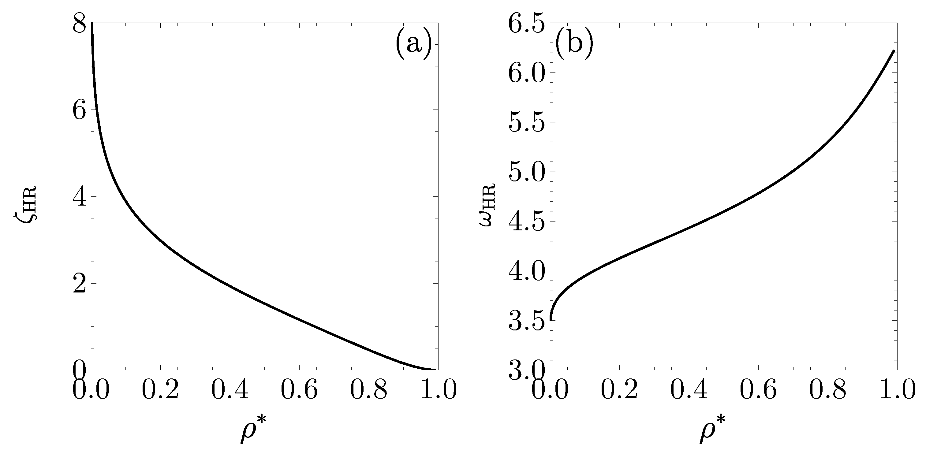
Regardless of the sign of , the leading pole at a given density in the high-temperature limit () is given by and , as shown in Appendix A.2, where the subscript HR refers to the hard-rod fluid. The HR oscillation frequency satisfies , with the lower and upper bounds corresponding to and , respectively. On the other hand, if and , the leading pole in the low-temperature limit () is given by and (see Appendix A.3.1). However, the low-temperature limit for is more intricate, as detailed in Appendix A.3.2.
If and real poles do exist, they are the solutions to
2.2. . Influence of on the DOC Line
In the case , the potential in Equation (1) simplifies to a hard core plus a square shoulder of width . The key question we aim to address is how the DOC line is affected as is varied.
As shown in Figure 1, the DOC line exhibits an intricate behavior as varies. For and , distinct DOC lines emerge, each starting at in the low-temperature region and shifting toward lower densities as the temperature increases. When , the DOC line intersects with a DOC loop at and . Inside the loop, the oscillation frequency reaches values , significantly larger than outside the loop. The intersection between the DOC line and the DOC loop acts as a triple point, where three distinct complex poles share the same real part, . An additional DOC arc appears, extending between and in the low-temperature region, within which reaches even higher values (, see Appendix A.3.2) than inside the DOC loop. For , the loop expands, shifting toward higher densities and lower temperatures, while the DOC arc broadens. Below (not shown in the figure), an inner arc emerges, which is absent in the case . In the region between the inner and outer arcs for , , whereas within the inner arc. As further decreases to , the original DOC line vanishes, with the loop and outer arc merging into a more complex DOC region (where ) and the inner arc region (where ) growing. At only the inner arc persists, with within. This evolution illustrates an increasingly complex pattern of structural transitions as the DOC line transforms with decreasing .
The insets in Figure 1 illustrate the temperature dependence of at several densities and values of . In the insets of Figure 1(a,b), transitions from at low to at high . In the inset of Figure 1(a), a single discontinuous shift is observed as the DOC line is traversed. However, in the inset of Figure 1(b), two distinct discontinuous jumps in occur as the DOC loop is crossed. The inset of Figure 1(c) shows two discontinuous drops in when crossing the DOC inner and outer arcs.
As further confirmation of the results presented in Figure 1, we numerically inverted the Laplace transform given by Equation (3) using the method described in [64] to obtain . The results for and four representative states are shown in Figure 2. In Figure 2(a–c), we fix the density and examine a temperature () below the loop, a temperature () inside the loop, and a temperature () above the loop. The corresponding leading poles are , , and , respectively, which align fully with the damped oscillatory behavior observed in Figure 2(a–c). As a representative state within the region between the inner and outer arcs, we considered and in Figure 2(d), for which .
2.3. , . Influence of on the DOC Line
If , both and become relevant parameters. For symmetry reasons, we will choose , so that both sections have the same width. As mentioned in Section 1, and to maintain concreteness, we will henceforth set and .
Figure 3(a) shows the DOC line, loop, and arc for [also displayed in Figure 1(b)] and for . In the latter case, the loop expands and shifts up and to the left, while the arc moves downward. For a fluid with [Figure 3(b)], the DOC line appears at a density below , with the loop evolving into a lobe that emerges from the vertical axis at . In Figure 3(c), a short DOC line forms at zero density when , but it vanishes when . As becomes increasingly negative, the DOC lobe progressively contracts, moving up and to the left until it eventually disappears (not shown). The insets in Figure 3 show the oscillation frequency as a function of at selected values of density and the energy ratio .
2.4. , , . Influence of on the FW Line
We now consider the case , where a genuine competition arises between the attractive square well with depth and the repulsive barrier of height . As demonstrated in Appendix A.1, real poles of may exist. If one of these real poles becomes dominant, the asymptotic decay of is monotonic, and, as mentioned earlier, an FW line emerges, marking the abrupt transition between monotonic and oscillatory decay. However, a DOC line may still occur, as exemplified by Figure 3(c).
The results for various values of are presented in Figure 4(a). A comparison of the DOC lines in Figure 3(c) for and with the corresponding FW lines in Figure 4(a) shows that the FW lines emerge at significantly lower values of and span a broader range of densities.
The strong sensitivity of the FW lines to the values of , as seen in Figure 4(a), is significantly reduced when temperature is scaled by the well depth , i.e., . This rescaling is applied in Figure 4(b), which also includes the FW line for a pure square-well fluid (). For the pure square-well fluid, the FW line approaches as (following a power law). However, introducing a repulsive barrier of height causes the FW line to bend at low densities, even when .
3. The 3D System: RFA Results
3.1. Theoretical Background
In this section, we provide a brief account of the main outcome of the RFA approach when the intermolecular potential in 3D is of the form of Equation (1). The detailed derivation may be found in References [20,22,24]. We begin by considering a function , which is distinct from its 1D counterpart. This function represents the Laplace transform of , specifically
We next define an auxiliary function directly related to through
where is the packing fraction. Taking into account Equations (3) and (4), we can say that is the 3D analog of the 1D quantity . To reflect the discontinuities of at the points , , and , where is discontinuous, we decompose as
Note that Equations (12)–(14) are formally exact. Finally, to construct our RFA, we assume the following rational-function approximate form for :
The approximation (15) contains nine parameters to be determined by application of certain constraints [20]. The expressions for those nine coefficients are presented in Appendix B.
Once again, the total correlation function can be expressed in terms of the nonzero poles of , which, in principle, form an infinite set. These poles may be either real or occur in complex-conjugate pairs. Their locations depend on the thermodynamic state, and as before, the pole with the real part closest to zero dictates the asymptotic behavior of the total correlation function for a given state. The 3D analogs of Equations (5) and (6) are, respectively,
In the context of the RFA, Equations (13)–(15) imply that the complex poles satisfy the following set of coupled equations:
with the convention . Analogously, the real poles are the roots of
It should be noted that the RFA results become less reliable at lower temperatures and/or higher densities. Therefore, we will primarily focus on cases where and . We now present our results following the same structure as in the 1D case (see Section 2).
3.2. . Influence of on the DOC Line
Figure 5(a) displays the DOC lines for 3D fluids with , corresponding to values of , , , , , and . The overall shape of these lines is qualitatively similar to the lines shown in Figure 1(b) for and , but with noticeably smaller loops, particularly as increases. Within these loops, as in the 1D case, the oscillation frequency is approximately . Furthermore, the DOC arcs observed in Figure 1(b,c) for 1D fluids are absent in Figure 5(a), as they would be confined to the high-density, low-temperature region where the RFA is no longer reliable. Indeed, no DOC line was observed for , consistent with the disappearance of the single DOC line in Figure 1(c) for and . Additionally, the 3D density playing the role of the 1D value would be given by , where represents the freezing density of hard spheres [65,66].
A comparison between Figure 5(b) and the inset of Figure 1(a) reveals a shared characteristic: when the single DOC line is crossed at a given density while moving from higher to lower temperatures, the frequency initially increases near the crossover temperature before suddenly dropping to a smaller value.
3.3. , . Influence of on the DOC Line
Figure 6(a) displays the DOC lines on the vs plane for various values of , covering the cases where , , and . In analogy with the 1D case [see Figure 3(b,c)], these lines exhibit qualitative changes as the system transitions from positive to negative values of . However, in the 3D case, apparently the loops do not degenerate into lobes.
Another notable feature is the rounded, bulging profile of the DOC lines for . This shape indicates that, within a certain density interval, the frequency exhibits reentrant behavior as the temperature varies. This phenomenon is illustrated in Figure 6(b) for . At a density (below the loop densities ), the oscillation frequency undergoes a single drop from to when crossing the temperature from left to right, and then increases smoothly toward in the high-temperature limit. At a higher density, (just below the bulge’s end at ), a more complex behavior is observed: the frequency drops from to at , then rises again from to at , eventually tending smoothly toward at high temperatures. Finally, at , the evolution of from at low temperatures to at high temperatures proceeds continuously without reentrant behavior.
3.4. , , . Influence of on the FW Line
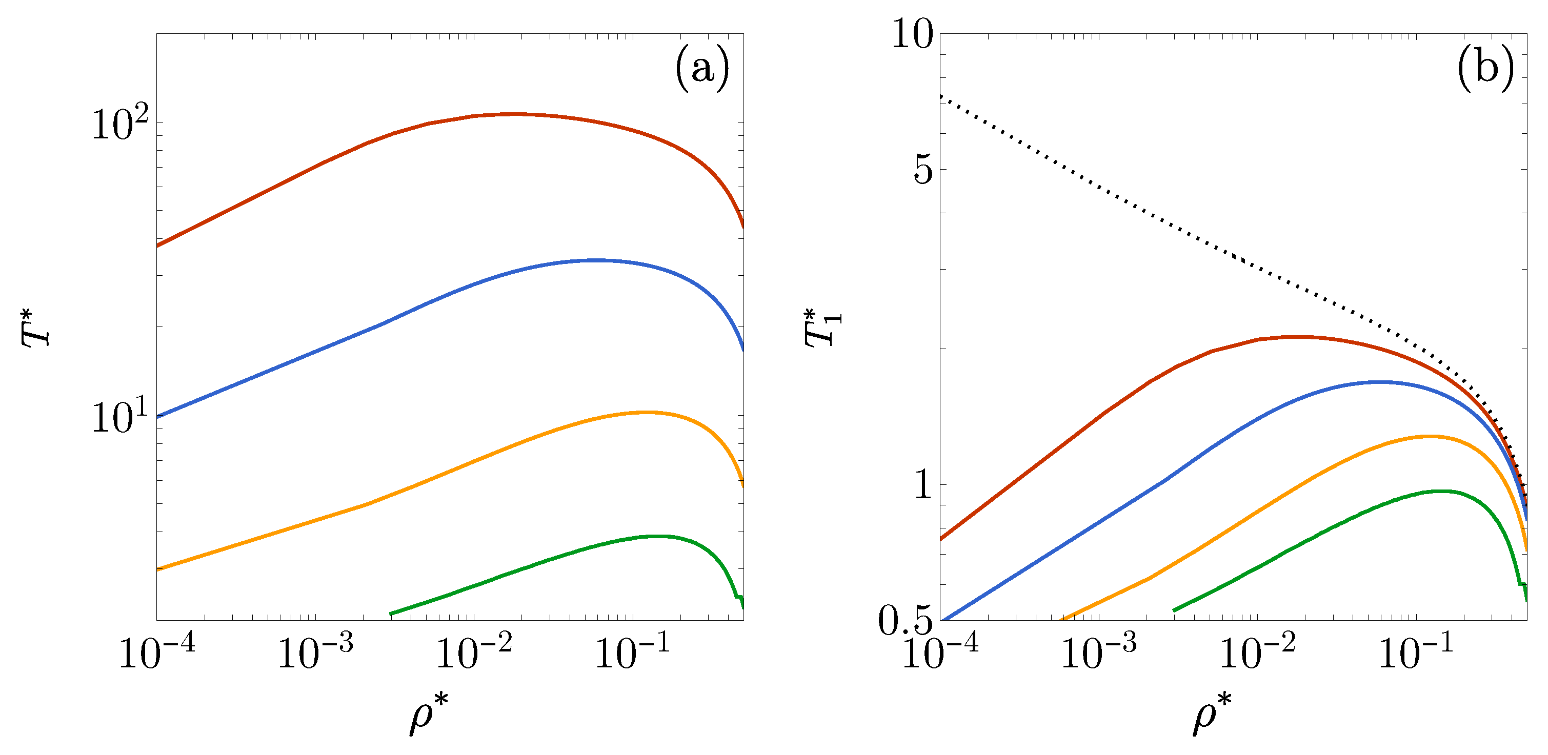
In the 1D case, an FW line was already observed with , but this required temperatures on the order of [see Figure 4(a)]. Since, as mentioned earlier, the RFA tends to provide less reliable results at low temperatures, it becomes necessary to consider deeper wells to study the FW lines for 3D fluids. The cases , , , and are reported in Figure 7(a). As in the 1D fluid, it is useful to plot the curves on the vs plane to compare them with the FW line of the pure square-well fluid, as shown in Figure 7(b). Again, we observe that the presence of the repulsive barrier between and bends the FW line downward in the low-density region. This indicates that the decay of is always oscillatory when the temperature exceeds a certain threshold, regardless of the density.
4. Conclusions
In this paper, we have explored the impact of competing interactions in the intermolecular potential of fluids on their structural transitions. The model potential adopted for both 1D and 3D systems consists of a hard core followed by two steps, which can represent either a shoulder or a well depending on the sign of the parameters and . This potential is versatile enough to encompass a range of competing interactions, including the square-well and square-shoulder interactions as limiting cases. Additionally, the consideration of two different dimensionalities allowed us to examine the influence of strong confinement on the structural transitions of these fluids. For the 1D systems, restricting the interaction range to no more than twice the hard-core diameter enabled us to derive exact results. In contrast, for the 3D systems, where exact solutions are not feasible, we employed the RFA to obtain and analyze approximate structural properties.
The results for both the 1D and 3D systems align with the expected behavior. Specifically, at very low temperatures, the decay of the total correlation function exhibits oscillations with a wavelength determined by the range of the repulsive barrier, provided that both and are positive. In contrast, at very high temperatures, the oscillations have a wavelength on the order of the hard-core diameter. Furthermore, it is confirmed that at a given density, the transition between these two regimes as the temperature increases can occur either continuously or, as observed in binary hard-sphere mixtures, discontinuously upon crossing a DOC line.
When is negative, an FW transition from an oscillatory to a monotonic decay of occurs as the temperature decreases at a given density, even when is positive. Additionally, the presence of the repulsive barrier of height causes the FW line to exhibit a maximum at a certain density before bending downward at lower densities, in stark contrast to its behavior in the absence of such a barrier.
While the results for both the 1D and 3D systems exhibit many common characteristic features, the effects of dimensionality introduce notable distinctions. These include shifts in the temperature ranges at which certain features appear, the need for deeper wells to observe similar phenomena, or a reduction in their prominence as the system transitions from 1D to 3D. In some cases, features present in 1D may vanish entirely in 3D. Notably, we emphasize the complex behavior of the DOC transition, as previously discussed. This intricacy manifests in phenomena such as loops, arcs, lobes, triple points, and reentrant frequencies—some of which, to the best of our knowledge, have not been reported in this context before.
In summary, we have uncovered a remarkably complex pattern of structural transitions in fluids with intermolecular potentials that include competing interactions. Even for the relatively simple potential considered in this work, analyzing structural transitions requires exploring a broad (dimensionless) parameter space, involving , , , , and . Given these circumstances, our findings should be viewed as an initial exploration—indicative but necessarily incomplete. Nonetheless, they highlight a fascinating and intricate phenomenology that warrants further and more detailed investigation.
Author Contributions
Conceptualization, A.S.; methodology, S.B.Y., A.S., and M.L.H.; software, A.M.M. and S.B.Y.; validation, A.M.M., S.B.Y., A.S., and M.L.H.; formal analysis, A.S. and M.L.H.; investigation, A.M.M., S.B.Y., A.S., and M.L.H.; writing—original draft preparation, A.S. and M.L.H; writing—review and editing, A.M.M., S.B.Y., A.S., and M.L.H.; visualization, A.M.M.; supervision, S.B.Y., A.S., and M.L.H.; funding acquisition, S.B.Y. and A.S. All authors have read and agreed to the published version of the manuscript.
Funding
This research was funded by MCIN/AEI/10.13039/501100011033 grant number PID2020-112936GB-I00. A.M.M. is grateful to the Spanish Ministerio de Ciencia e Innovación for a predoctoral fellowship Grant No. PRE2021-097702.
Data Availability Statement
The raw data supporting the conclusions of this article will be made available by the authors on request.
Conflicts of Interest
The authors declare no conflicts of interest.
Abbreviations
The following abbreviations are used in this manuscript:
| 1D | One-dimensional |
| 3D | Three-dimensional |
| DOC | Discontinuous Oscillation Crossover |
| FW | Fisher–Widom |
| HR | Hard-rod |
| RFA | Rational Function Approximation |
Appendix A. Some Mathematical Details in the Case of the 1D Fluid
Appendix A.1. Absence of Real Poles if φ(r)≥0
We first consider a generic potential that goes to ∞ if and vanishes if . If a real pole of exists, then
If s is real and positive, decreases monotonically with s. Consequently, Equation (A1) cannot be satisfied for . If, on the other hand, , the argument becomes negative and, thus, we first need to evaluate assuming that and then perform an analytic continuation to . With ,
This expression can now be analytically continued to . Therefore, if , we can write
If , then . In that case, and given that , one has and Equation (A1) cannot be satisfied.
In summary, if for all r, then no real poles exist. Otherwise, real poles may exist but, then, .
Appendix A.2. Poles in the High-Temperature Limit
In the limit , the system simplifies to a HR fluid with diameter . In this regime, Equations (9) and (10) reduce to
By squaring both sides of the equalities in Equation (A4b) and adding them, can be expressed as a function of :
Substituting this expression into the first equality of Equation (A4b) yields a closed equation for , which can be solved numerically to find the pole with the smallest value of . It is important to discard any spurious root that may appear for as a consequence of squaring the equations.
In the close-packing limit , it is easy to obtain
On the other hand, in the opposite low-density limit () one has and . The latter belongs to the class of Lambert equations with and . The solution is then
where is the lower branch of the Lambert function [67]. The functions and are plotted in Figure A1
Figure A1.
Density dependence of (a) and (b) .
Appendix A.3. Poles in the Low-Temperature Limit with ϵ 1 >0
Appendix A.3.1. Case 0<ρ * <λ 2 -1
In the low-temperature limit with , one can see from Equations (7)–(10) that the system becomes equivalent to an HR fluid with diameter , provided that . Therefore, in that limit one has
Appendix A.3.2. Case λ 2 -1 <ρ * <1
In the limit with finite p one has , so that Equation (9) yields
The dominant terms in Equation (A9) depend on the domain of p. One can distinguish three possibilities. First, if
one has . Next, if
the result is . Finally, if
then .
Suppose first that . In that case, the inequalities in (A10) and (A11) imply and , respectively, while the inequality in (A12) is impossible. Thus, in the low-temperature limit, the density changes from to as pressure crosses the value . To analyze this change in detail, let us introduce the scaled variable by
so that Equation (A9) becomes
In turn, from Equations (A9) we have
For simplicity, let us assume that is a rational number . The analytical solution to Equations (A15) in the limit is displayed in the first row of Table A1.

Table A1.
Asymptotic expressions for p, , and in the low-temperature limit for 1D fluids with , assuming , , and are rational numbers.
Table A1.
Asymptotic expressions for p, , and in the low-temperature limit for 1D fluids with , assuming , , and are rational numbers.
| p | ||||
|---|---|---|---|---|
In contrast, for a potential where , the situation becomes more intricate. In this case, the inequalities in Equations (A10), (A11), and (A12) imply the following conditions: , , and , respectively. This indicates that, in the low-temperature limit, the density changes from to as the pressure crosses , and from to as the pressure crosses . An analysis similar to that conducted in Equations (A13)–(A15) leads to the expressions shown in the second and third rows of Table A1. An oscillation discontinuity at only arises if , meaning must be an integer. This condition excludes cases such as and , where , , , , , and .
Appendix B. Parameters in Equation (15)
First, the exact condition for small s yields
Here,
Further, since the cavity function must be continuous at and , the two following conditions should also hold [20]
where () are the three roots of the cubic equation .
Equations (A16)–(A18) still leave two parameters undetermined. A simplifying assumption is that the coefficients () may be fixed at their zero-density values, namely
This closes the problem of determining the nine parameters in terms of , , , , and . In fact, Equations (A16) allow us to express , , , and as linear combinations of and , so that in the end one only has to solve (numerically) the two coupled transcendental Equation (A18).
References
- McQuarrie, D.A. Statistical Mechanics; Harper & Row: New York, 1976.
- Chapela, G.A.; Martínez-Casas, S.E.; Alejandre, J. Molecular dynamics for discontinuous potentials. I. General method and simulation of hard polyatomic molecules. Mol. Phys. 1984, 53, 139–159. [Google Scholar] [CrossRef]
- Chapela, G.A.; Scriven, L.E.; Davis, H.T. Molecular dynamics for discontinuous potential. IV. Lennard-Jonesium. J. Chem. Phys. 1989, 91, 4307–4313. [Google Scholar] [CrossRef]
- Benavides, A.L.; Gil-Villegas, A. The thermodynamics of molecules with discrete potentials. Mol. Phys. 1999, 97, 1225–1232. [Google Scholar] [CrossRef]
- Franzese, G.; Malescio, G.; Skibinsky, A.; Buldyrev, S.V.; Stanley, H.E. Generic mechanism for generating a liquid-liquid phase transition. Nature 2001, 409, 692–695. [Google Scholar] [CrossRef] [PubMed]
- Malescio, G.; Franzese, G.; Pellicane, G.; Skibinsky, A.; Buldyrev, S.V.; Stanley, H.E. Liquid-liquid phase transition in one-component fluids. J. Phys.: Condens. Matter 2002, 14, 2193–2200. [Google Scholar] [CrossRef]
- Skibinsky, A.; Buldyrev, S.V.; Franzese, G.; Malescio, G.; Stanley, H.E. Liquid-liquid phase transitions for soft-core attractive potentials. Phys. Rev. E 2004, 69, 061206. [Google Scholar] [CrossRef]
- Malescio, G.; Franzese, G.; Skibinsky, A.; Buldyrev, S.V.; Stanley, H.E. Liquid-liquid phase transition for an attractive isotropic potential with wide repulsive range. Phys. Rev. E 2005, 71, 061504. [Google Scholar] [CrossRef]
- Benavides, A.L.; del Pino, L.A.; Gil-Villegas, A.; Sastre, F. Thermodynamic and structural properties of confined discrete-potential fluids. J. Chem. Phys. 2006, 125, 204715. [Google Scholar] [CrossRef]
- Cervantes, L.A.; Benavides, A.L.; del Río, F. Theoretical prediction of multiple fluid-fluid transitions in monocomponent fluids. J. Chem. Phys. 2007, 126, 084507. [Google Scholar] [CrossRef]
- Guillén-Escamilla, I.; Chávez-Páez, M.; Castañeda-Priego, R. Structure and thermodynamics of discrete potential fluids in the OZ-HMSA formalism. J. Phys.: Condens. Matter 2007, 19, 086224. [Google Scholar] [CrossRef]
- Rżysko, W.; Pizio, O.; Patrykiejew, A.; Sokolowski, S. Phase diagram of a square-shoulder, square-well fluid revisited. J. Chem. Phys. 2008, 129, 124502. [Google Scholar] [CrossRef] [PubMed]
- de Oliveira, A.B.; Franzese, G.; Netz, P.A.; Barbosa, M.C. Waterlike hierarchy of anomalies in a continuous spherical shouldered potential. J. Chem. Phys. 2008, 128, 064901. [Google Scholar] [CrossRef] [PubMed]
- de Oliveira, A.B.; Netz, P.A.; Barbosa, M.C. An ubiquitous mechanism for water-like anomalies. EPL 2009, 85, 36001. [Google Scholar] [CrossRef]
- Rżysko, W.; Patrykiejew, A.; Sokołowski, S.; Pizio, O. Phase behavior of a two-dimensional and confined in slitlike pores square-shoulder, square-well fluid. J. Chem. Phys. 2010, 132, 164702. [Google Scholar] [CrossRef]
- Hlushak, S.P.; Trokhymchuk, A.D.; Sokołowski, S. Direct correlation function for complex square barrier-square well potentials in the first-order mean spherical approximation. J. Chem. Phys. 2011, 134, 114101. [Google Scholar] [CrossRef]
- Yuste, S.B.; Santos, A.; López de Haro, M. Structure of the square-shoulder fluid. Mol. Phys. 2011, 109, 987–995. [Google Scholar] [CrossRef]
- Bárcenas, M.; Odriozola, G.; Orea, P. Propiedades termodinámicas de fluidos de hombro/pozo cuadrado. Rev. Mex. Fís. 2011, 57, 485–490. [Google Scholar]
- Loredo-Osti, A.; Castañeda-Priego, R. Analytic Structure Factor of Discrete Potential Fluids: Cluster-Like Correlations and Micro-Phases. J. Nanofluids 2012, 1, 36–43. [Google Scholar] [CrossRef]
- Santos, A.; Yuste, S.B.; López de Haro, M. Rational-function approximation for fluids interacting via piece-wise constant potentials. Condens. Matter Phys. 2012, 15, 23602. [Google Scholar] [CrossRef]
- Bárcenas, M.; Odriozola, G.; Orea, P. Structure and coexistence properties of shoulder-square well fluids. J. Mol. Liq. 2013, 185, 70–75. [Google Scholar] [CrossRef]
- Santos, A.; Yuste, S.B.; López de Haro, M.; Bárcenas, M.; Orea, P. Structural properties of fluids interacting via piece-wise constant potentials with a hard core. J. Chem. Phys. 2013, 139, 074505. [Google Scholar] [CrossRef] [PubMed]
- Kim, E.Y.; Kim, S.C. Structure of discrete-potential fluids interacting via two piece-wise constant potentials with a hard-core. J. Mol. Liq. 2013, 187, 326–331. [Google Scholar] [CrossRef]
- Yuste, S.B.; Santos, A.; López de Haro, M. Structural and thermodynamic properties of fluids whose molecules interact via one-, two-, and three-step potentials. J. Mol. Liq. 2022, 364, 119890. [Google Scholar] [CrossRef]
- Perdomo-Pérez, R.; Martínez-Rivera, J.; Palmero-Cruz, N.C.; Sandoval-Puentes, M.A.; Gallegos, J.A.S.; Lázaro-Lázaro, E.; Valadez-Pérez, N.E.; Torres-Carbajal, A.; Castañeda-Priego, R. Thermodynamics, static properties and transport behaviour of fluids with competing interactions. J. Phys.: Condens. Matter 2022, 34, 144005. [Google Scholar] [CrossRef] [PubMed]
- Largo, J.; Solana, J.R. Liquid-liquid transition in a simple model fluid with competitive interactions. Mol. Phys. 2014, p. e2356756. [CrossRef]
- Ruiz-Franco, J.; Zaccarelli, E. On the Role of Competing Interactions in Charged Colloids with Short-Range Attraction. Annu. Rev. Condens. Matter Phys. 2021, 12, 51–70. [Google Scholar] [CrossRef]
- Kravtsiv, I.; Patsahan, T.; Holovko, M.; di Caprio, D. Soft core fluid with competing interactions at a hard wall. J. Mol. Liq. 2022, 362, 119652. [Google Scholar] [CrossRef]
- Carretas-Talamante, A.G.; Zepeda-López, J.B.; Lázaro-Lázaro, E.; Elizondo-Aguilera, L.F.; Medina-Noyola, M. Non-equilibrium view of the amorphous solidification of liquids with competing interactions. J. Chem. Phys. 2023, 158, 064506. [Google Scholar] [CrossRef]
- Tan, Z.; Calandrini, V.; Dhont, J.K.G.; Nägele, G. Quasi-two-dimensional dispersions of Brownian particles with competitive interactions: phase behavior and structural properties. Soft Matter 2024. [Google Scholar] [CrossRef]
- Imperio, A.; Reatto, L. Microphase separation in two-dimensional systems with competing interactions. J. Chem. Phys. 2006, 124, 164712. [Google Scholar] [CrossRef]
- Archer, A.J.; Wilding, N.B. Phase behavior of a fluid with competing attractive and repulsive interactions. Phys. Rev. E 2007, 76, 031501. [Google Scholar] [CrossRef]
- Bomont, J.M.; Bretonnet, J.L.; Costa, D.; Hansen, J.P. Communication: Thermodynamic signatures of cluster formation in fluids with competing interactions. J. Chem. Phys. 2012, 137, 011101. [Google Scholar] [CrossRef] [PubMed]
- Bollinger, J.A.; Truskett, T.M. Fluids with competing interactions. I. Decoding the structure factor to detect and characterize self-limited clustering. J. Chem. Phys. 2016, 145, 064902. [Google Scholar] [CrossRef]
- Bollinger, J.A.; Truskett, T.M. Fluids with competing interactions. II. Validating a free energy model for equilibrium cluster size. J. Chem. Phys. 2016, 145, 064903. [Google Scholar] [CrossRef]
- Hu, Y.; Charbonneau, P. Clustering and assembly dynamics of a one-dimensional microphase former. Soft Matter 2018, 14, 4101–4109. [Google Scholar] [CrossRef] [PubMed]
- Malescio, G.; Sciortino, F. Aggregate formation in fluids with bounded repulsive core and competing interactions. J. Mol. Liq. 2020, 303, 12601. [Google Scholar] [CrossRef]
- Bomont, J.M.; Costa, D.; Bretonnet, J.L. Local order and cluster formation in model fluids with competing interactions: a simulation and theoretical study. Phys. Chem. Chem. Phys. 2020, 22, 5355–5365. [Google Scholar] [CrossRef]
- Guillén-Escamilla, I.; Méndez-Bermúdez, J.G.; Mixteco-Sánchez, J.C.; Méndez-Maldonado, G.A. Microphase and macrophase separations in discrete potential fluids. Rev. Mex. Fís. 2022, 68, 050502. [Google Scholar] [CrossRef]
- Munaò, G.; Costa, D.; Malescio, G.; Bomont, J.M.; Prestipino, S. Competition between clustering and phase separation in binary mixtures containing SALR particles. Soft Matter 2022, 18, 6453–6464. [Google Scholar] [CrossRef]
- Munaò, G.; Prestipino, S.; Bomont, J.M.; Costa. Clustering in Mixtures of SALR Particles and Hard Spheres with Cross Attraction. J. Phys. Chem. B 2022, 126, 2027–2039. [Google Scholar] [CrossRef]
- Costa, D.; Munaò, G.; Bomont, J.M.; Malescio, G.; Palatella, A.; Prestipino, S. Microphase versus macrophase separation in the square-well-linear fluid: A theoretical and computational study. Phys. Rev. E 2023, 108, 034602. [Google Scholar] [CrossRef]
- Bomont, J.M.; Pastore, G.; Costa, D.; Munaò, G.; Malescio, G.; Prestipino, S. Arrested states in colloidal fluids with competing interactions: A static replica study. J. Chem. Phys. 2024, 160, 214504. [Google Scholar] [CrossRef] [PubMed]
- López de Haro, M.; Yuste, S.B.; Santos, A. Alternative Approaches to the Equilibrium Properties of Hard-Sphere Liquids. In Proceedings of the Theory and Simulation of Hard-Sphere Fluids and Related Systems; Mulero, A., Ed., Berlin, 2008; Vol. 753, Lecture Notes in Physics, pp. 183–245. [CrossRef]
- Santos, A. A Concise Course on the Theory of Classical Liquids. Basics and Selected Topics; Vol. 923, Lecture Notes in Physics, Springer: New York, 2016. [CrossRef]
- Pieprzyk, S.; Brańka, A.C.; Yuste, S.B.; Santos, A.; López de Haro, M. Structural properties of additive binary hard-sphere mixtures. Phys. Rev. E 2020, 101, 012117. [Google Scholar] [CrossRef] [PubMed]
- Pieprzyk, S.; Yuste, S.B.; Santos, A.; López de Haro, M.; Brańka, A.C. Structural properties of additive binary hard-sphere mixtures. II. Asymptotic behavior and structural crossovers. Phys. Rev. E 2021, 104, 024128. [Google Scholar] [CrossRef] [PubMed]
- Pieprzyk, S.; Yuste, S.B.; Santos, A.; López de Haro, M.; Brańka, A.C. Structural properties of additive binary hard-sphere mixtures. III. Direct correlation functions. Phys. Rev. E 2021, 104, 054142. [Google Scholar] [CrossRef]
- Grodon, C.; Dijkstra, M.; Evans, R.; Roth, R. Decay of correlation functions in hard-sphere mixtures: Structural crossover. J. Chem. Phys. 2004, 121, 7869–7882. [Google Scholar] [CrossRef]
- Grodon, C.; Dijkstra, M.; Evans, R.; Roth, R. Homogeneous and inhomogeneous hard-sphere mixtures: manifestations of structural crossover. Mol. Phys. 2005, 103, 3009–3023. [Google Scholar] [CrossRef]
- Statt, A.; Pinchaipat, R.; Turci, F.; Evans, R.; Royall, C.P. Direct observation in 3d of structural crossover in binary hard sphere mixtures. J. Chem. Phys. 2016, 144, 144506. [Google Scholar] [CrossRef]
- Royall, C.P.; Charbonneau, P.; Dijkstra, M.; Russo, J.; Smallenburg, F.; Speck, T.; Valeriani, C. Colloidal hard spheres: Triumphs, challenges, and mysteries. Rev. Mod. Phys. 2024, 96, 045003. [Google Scholar] [CrossRef]
- Salsburg, Z.W.; Zwanzig, R.W.; Kirkwood, J.G. Molecular distribution functions in a one-dimensional fluid. J. Chem. Phys. 1953, 21, 1098–1107. [Google Scholar] [CrossRef]
- Lebowitz, J.L.; Zomick, D. Mixtures of hard spheres with nonadditive diameters: Some exact results and solution of PY equation. J. Chem. Phys. 1971, 54, 3335–3346. [Google Scholar] [CrossRef]
- Percus, J.K. Equilibrium state of a classical fluid of hard rods in an external field. J. Stat. Phys. 1976, 15, 505–511. [Google Scholar] [CrossRef]
- Percus, J.K. One-dimensional classical fluid with nearest-neighbor interaction in arbitrary external field. J. Stat. Phys. 1982, 28, 67–81. [Google Scholar] [CrossRef]
- Heying, M.; Corti, D.S. The one-dimensional fully non-additive binary hard rod mixture: exact thermophysical properties. Fluid Phase Equilib. 2004, 220, 85–103. [Google Scholar] [CrossRef]
- Santos, A. Exact bulk correlation functions in one-dimensional nonadditive hard-core mixtures. Phys. Rev. E 2007, 76, 062201. [Google Scholar] [CrossRef]
- Ben-Naim, A.; Santos, A. Local and global properties of mixtures in one-dimensional systems. II. Exact results for the Kirkwood–Buff integrals. J. Chem. Phys. 2009, 131, 164512. [Google Scholar] [CrossRef]
- Fantoni, R.; Santos, A. One-Dimensional Fluids with Second Nearest-Neighbor Interactions. J. Stat. Phys. 2017, 169, 1171–1201. [Google Scholar] [CrossRef]
- Montero, A.M.; Santos, A. Triangle-Well and Ramp Interactions in One-Dimensional Fluids: A Fully Analytic Exact Solution. J. Stat. Phys. 2019, 175, 269–288. [Google Scholar] [CrossRef]
- Maestre, M.A.G.; Santos, A. One-dimensional Janus fluids. Exact solution and mapping from the quenched to the annealed system. J. Stat. Mech. 2020, 2020, 063217. [Google Scholar] [CrossRef]
- Montero, A.M.; Rodríguez-Rivas, A.; Yuste, S.B.; Santos, A.; López de Haro, M. On a conjecture concerning the Fisher–Widom line and the line of vanishing excess isothermal compressibility in simple fluids. Mol. Phys. 2024, p. e2357270. [CrossRef]
- Yuste, S.B. Numerical Inversion of Laplace Transforms using the Euler Method of Abate and Whitt. https://github.com/SantosBravo/Numerical-Inverse-Laplace-Transform-Abate-Whitt, 2023. It is convenient to assign to the parameter ntr values larger than x.
- Alder, B.J.; Wainwright, T.E. Phase Transition for a Hard Sphere System. J. Chem. Phys. 1957, 27, 1208–1209. [Google Scholar] [CrossRef]
- Robles, M.; López de Haro, M.; Santos, A. Note: Equation of state and the freezing point in the hard-sphere model. J. Chem. Phys. 2014, 140, 136101. [Google Scholar] [CrossRef]
- Corless, R.M.; Gonnet, G.H.; Hare, D.E.G.; Jeffrey, D.J.; Knuth, D.E. On the Lambert W function. Adv. Comput. Math. 1996, 5, 329–359. [Google Scholar] [CrossRef]
Figure 1.
DOC lines on the vs plane for the 1D case with : (a) , (b) , and (c) . Insets display the angular frequency of the asymptotic oscillations of as a function of for (a) at , (b) at , and (c) at .
Figure 1.
DOC lines on the vs plane for the 1D case with : (a) , (b) , and (c) . Insets display the angular frequency of the asymptotic oscillations of as a function of for (a) at , (b) at , and (c) at .
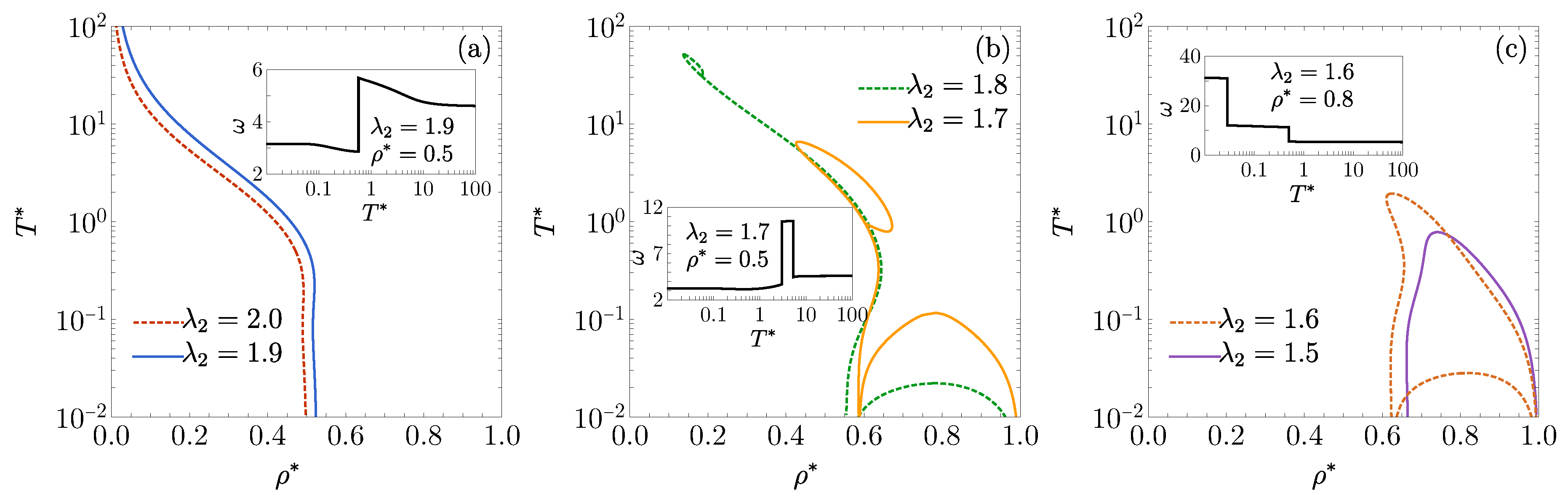
Figure 2.
Logarithmic plot of for large r in the 1D case , , for the following states: (a) , (b) , (c) , and (d) .
Figure 2.
Logarithmic plot of for large r in the 1D case , , for the following states: (a) , (b) , (c) , and (d) .
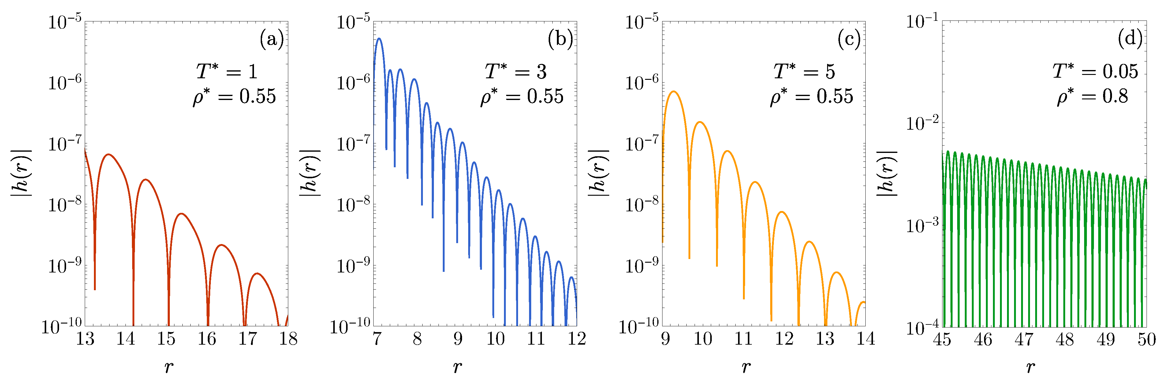
Figure 3.
DOC lines on the vs plane for the 1D case with and : (a) , (b) , and (c) . Insets display the angular frequency of the asymptotic oscillations of as a function of for (a) at , (b) at , and (c) at .
Figure 3.
DOC lines on the vs plane for the 1D case with and : (a) , (b) , and (c) . Insets display the angular frequency of the asymptotic oscillations of as a function of for (a) at , (b) at , and (c) at .
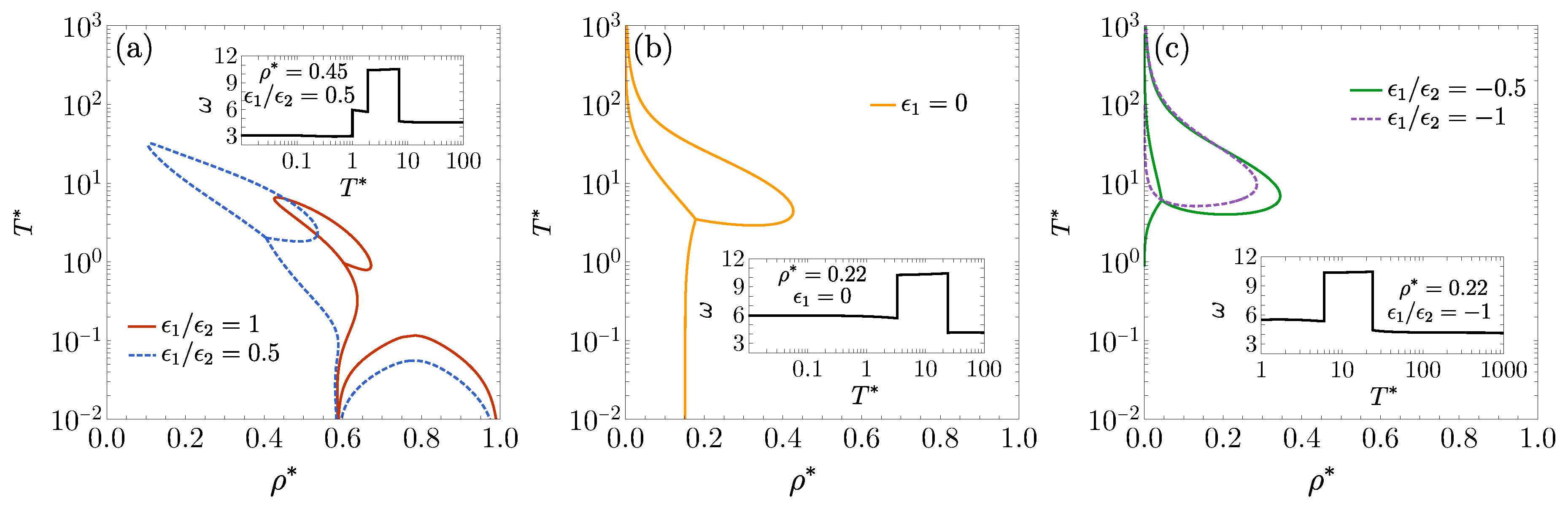
Figure 4.
(a) FW lines on the vs plane for the 1D case and with, from bottom to top, , , , , , and . (b) Same as in panel (a), except that now the vertical axis represents the scaled temperature . The dotted curve is the FW line for a pure square-well fluid (). Note that in panel (b) the curves corresponding to and are indistinguishable.
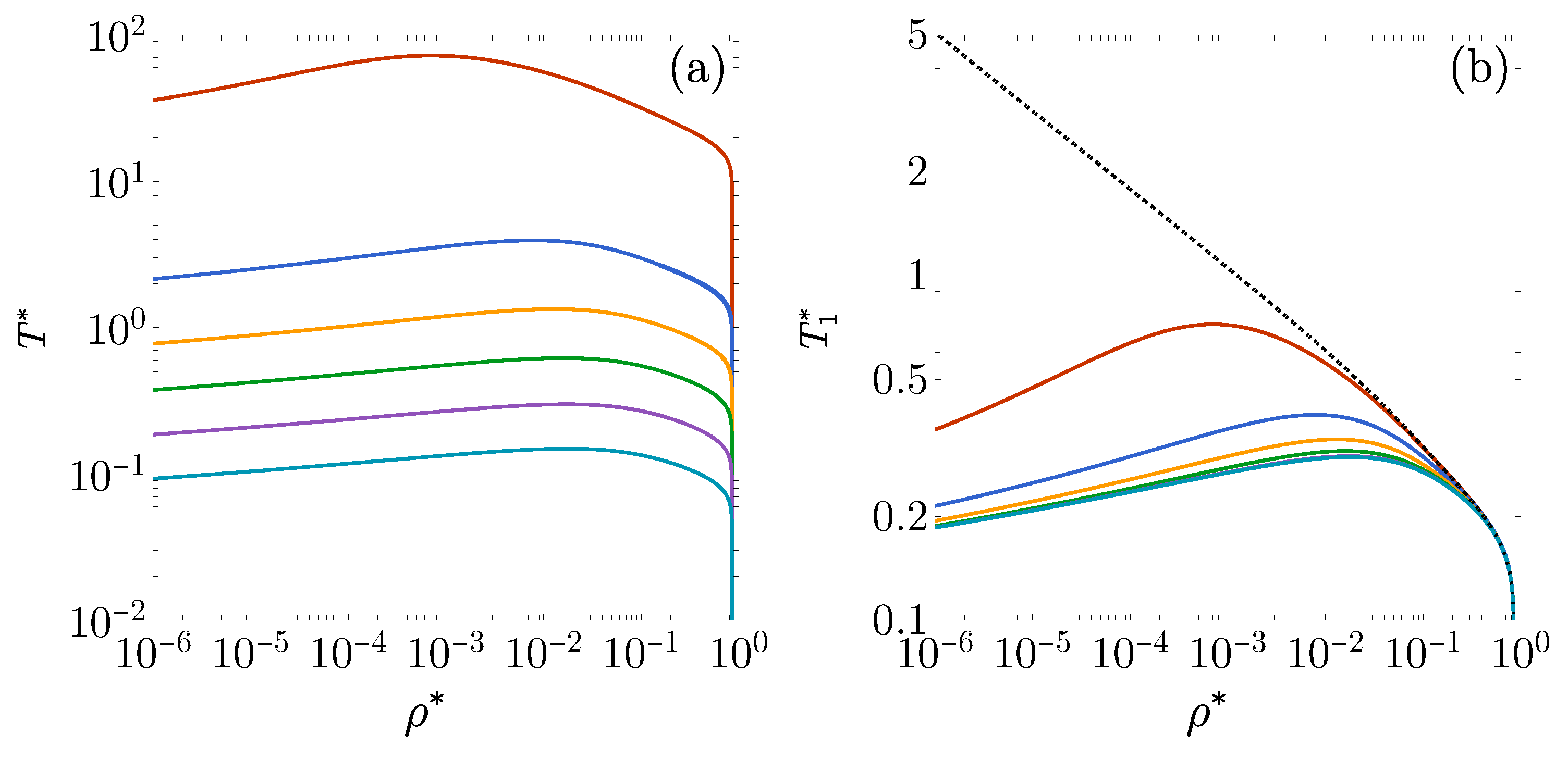
Figure 5.
(a) DOC lines on the vs plane for the 3D case with , , , , , and . The inset shows the loop corresponding to . (b) Angular frequency of the asymptotic oscillations of plotted as a function of for , , , , , , and , with an interaction potential characterized by and . The arrows indicate the direction of increasing (a) and (b) .
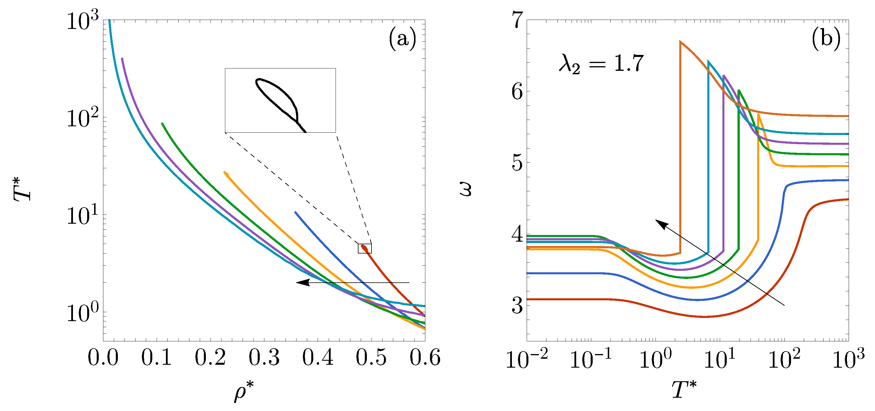
Figure 6.
(a) DOC lines on the vs plane for the 3D case and with, from right to left, , 2, 1, , 0, , , , and . The inset shows the loop corresponding to . (b) Angular frequency of the asymptotic oscillations of plotted as a function of for , , and , with an interaction potential characterized by , , and .
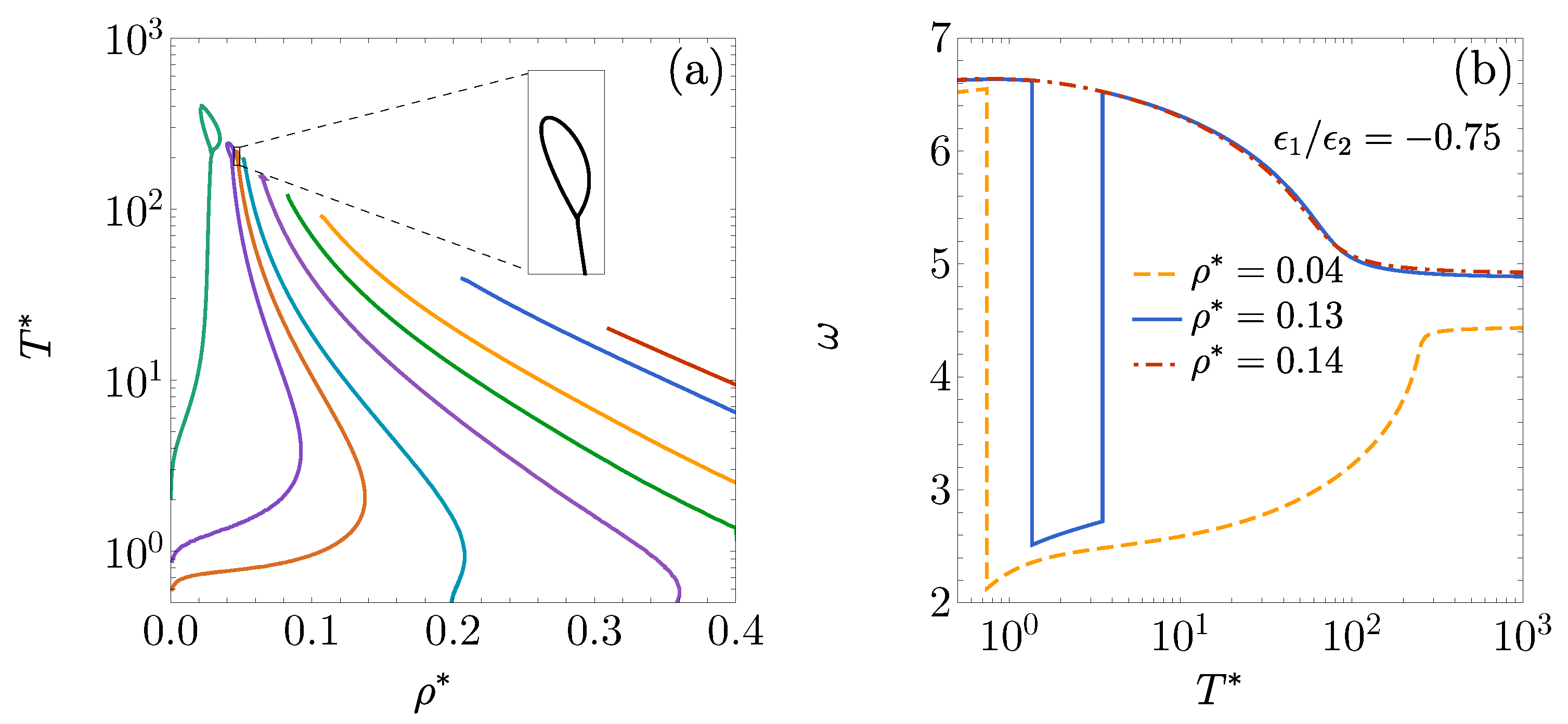
Figure 7.
(a) FW lines on the vs plane for the 3D case and with, from bottom to top, , , , and . (b) Same as in panel (a), except that now the vertical axis represents the scaled temperature . The dotted line is the FW line for a pure square-well fluid ().
Figure 7.
(a) FW lines on the vs plane for the 3D case and with, from bottom to top, , , , and . (b) Same as in panel (a), except that now the vertical axis represents the scaled temperature . The dotted line is the FW line for a pure square-well fluid ().
Disclaimer/Publisher’s Note: The statements, opinions and data contained in all publications are solely those of the individual author(s) and contributor(s) and not of MDPI and/or the editor(s). MDPI and/or the editor(s) disclaim responsibility for any injury to people or property resulting from any ideas, methods, instructions or products referred to in the content. |
© 2024 by the authors. Licensee MDPI, Basel, Switzerland. This article is an open access article distributed under the terms and conditions of the Creative Commons Attribution (CC BY) license (http://creativecommons.org/licenses/by/4.0/).
Copyright: This open access article is published under a Creative Commons CC BY 4.0 license, which permit the free download, distribution, and reuse, provided that the author and preprint are cited in any reuse.


