
Submitted:
13 May 2025
Posted:
13 May 2025
You are already at the latest version
Abstract
Predicted natural ventilation (NV) often diverges from actual performance in dwellings. This discrepancy arises in part because most design tools do not account for how occupants actually operate windows. This study aims to determine how window geometry and orientation should be adjusted when occupant behavior is considered. Survey data from 150 Melbourne residents were converted into two window-operation schedules: Same Behavior (SB), representing average patterns, and Probable Behavior (PB), capturing stochastic responses to comfort, privacy, and climate. Both schedules were embedded in EnergyPlus and applied to over 200 annual simulations across five window design stories that varied orientations, placements, and window-to-wall ratios (WWR). Each story was tested across two living room wall dimensions (7 m and 4.5 m) and evaluated for air-change rate per hour (ACH) and solar gains. PB increased annual ACH by 5–12 % over SB, with the greatest uplift in north-facing cross-ventilated layouts on the wider wall. Integrating probabilistic occupant behavior into window design remarkably improves NV effectiveness, with peak summer ACH reaching 4.8, indicating high ventilation rates that support thermal comfort and improved IAQ without mechanical assistance. These results highlight the potential of occupant-responsive window configurations to reduce reliance on mechanical cooling and enhance indoor air quality (IAQ). The study contributes a replicable occupant-centered workflow and ready-to-apply design rules for Australian temperate climates, adapted to different climate zones. Future research will extend the method to different climates, housing types, and user profiles, and integrate smart-sensor feedback, adaptive glazing, and hybrid ventilation strategies through multi-objective optimization.
Keywords:
indoor air quality (iaq)
; natural ventilation (nv)
; occupants' behavior
; occupants' perceptions
; window design
1. Introduction
Despite progressive building codes, sophisticated simulation tools [1], and increasingly ambitious energy-efficiency targets, a significant gap [2] often exists between predicted and actual measured building performance [3,4]. While inaccuracies due to construction practices and simplified modelling assumptions explain part of the discrepancy [5], recent field studies consistently highlight occupant behavior [6] as the significant yet overlooked factor influencing real-world outcomes [7,8,9]. In Australia, rating systems such as the Nationwide House Energy Rating Scheme (NatHERS) acknowledge occupant-related factors, but their standard schedules rarely reflect the day-to-day variability of human decisions that directly shape indoor environmental quality (IEQ) and energy usage [10,12].
Among occupant-controlled actions, window operation has the most immediate and profound influence on natural ventilation (NV), indoor air quality (IAQ), and thermal comfort [13,14]. Unlike thermostat adjustments [15], shading control [16], or fan use, window interactions directly mediate airflow between indoor and outdoor environments [17,18,19]. Window opening decisions are influenced by diverse personal, cultural, climatic, and socio-economic factors, such as energy cost sensitivity, housing type and density, and occupants’ awareness [20,21,22]. The COVID-19 lockdowns amplified awareness of the health implications of inadequate ventilation and further highlighted the critical role windows play in maintaining safe and comfortable indoor environments [23,24,25].
While geometric characteristics, such as orientation, size, placement, operability [26,27], and window-to-wall ratio (WWR) [28,29], inherently determine ventilation potential, these features also significantly influence occupant behavior [30,31]. For instance, larger and well-oriented openings can physically facilitate higher air-change rates [32,33,34], yet can unintentionally introduce excessive solar heat gains [35], a trade-off examined in studies on energy performance optimization in various climates [36,37,38]. Current standard simulation practices simplify these complex interactions by relying on static, rule-based schedules [39,40], ignoring the dynamic, adaptive nature of occupant responses, such as thermal comfort or privacy-driven behaviors, explored in previous studies [17,18]. Agent-based models, like those developed in the literature [41], attempt to capture more realism, but common simulation practices still struggle with behavioral nuances [42,43]. Consequently, many design recommendations mis-predict real-world NV performance [44,45], especially in mild temperate climates where window use is highly variable and adaptive comfort models are crucial [46,47].
Effectively closing this performance gap requires more integrated, behavior-aware modelling workflows that combine empirical occupant observations, such as those gathered from surveys and post-occupancy evaluations (POE) [48,49,50], which reveal occupant preferences and actions [17,51], with computational tools like Computational Fluid Dynamics (CFD) [31,52] and energy models that assess physical performance [53,54]. Furthermore, emerging data-driven techniques, such as Artificial Intelligence (AI) in building energy management [55], machine learning models predicting occupancy and window use [56,57], and multi-criteria decision methods (MCDM) for evaluating complex systems [58,59], offer powerful ways to analyze these interactions. Such hybrid approaches can reveal how occupants respond to thermal and visual cues [60,61], and how window geometry can nudge them towards healthier and more energy-efficient patterns [62,63]. However, existing studies have not combined empirical behavior models with systematic window design exploration in a replicable simulation-based framework. Although these sophisticated methods exist, practical integration into current design practices remains limited. This highlights the need for straightforward yet realistic simulation approaches that blend detailed occupant insights with proven simulation tools to provide clear, actionable guidance on how window designs influence real occupant behaviors and NV performance.
Addressing this critical gap, the present study introduces a novel user-centric simulation framework, explicitly coupling probabilistic occupant behavior models derived from empirical surveys with systematic window design exploration. Adapted to Australian temperate climates, this approach leverages two distinct window-operation schedules, Same Behavior (SB), reflecting typical use patterns, and Probable Behavior (PB), capturing more realistic occupant variability, and evaluates them within the EnergyPlus simulation environment. Through more than 200 annual simulations, this research aims to answer two main questions: (i) Which specific window design attributes most enhance NV when real occupant actions are considered? and (ii) How much does incorporating realistic occupant behavior (PB) improve ventilation outcomes compared to standard simulation assumptions (SB)? By quantifying these links, the study offers new, ready-to-apply design rules tailored for behavior-integrated window design, helping architects and engineers narrow the ventilation performance gap in residential buildings [64,65]. The following sections detail the survey methodology, simulation framework (Section 2), results and practical implications (Section 3), discuss limitations and directions for future research (Section 4), and conclude by summarizing key insights and recommendations (Section 5).
2. Methodology
This study deploys a behavior-integrated simulation framework to explore how window design features and real-world occupants collectively affect NV performance in residential buildings located in the temperate climate of Melbourne, Australia. Two distinct occupant-window operation schedules were developed based on survey data from 150 Melbourne households [20]:
- Same Behavior (SB): a deterministic schedule representing average occupant behavior.
- Probable Behavior (PB): a stochastic (probabilistic) schedule capturing variations due to factors like comfort, privacy, and climate conditions. PB was derived by assigning time-of-day-dependent probabilities to window actions based on survey responses; no thermal comfort models (e.g., Fanger) were used. Further details are available in Appendix A.
Both schedules were integrated into EnergyPlus simulations to quantify their impacts on air-change rate per hour (ACH), indoor temperatures, and solar gains. Five distinct window-design scenarios, named stories, including different orientations, placements, and WWR = 0.25–0.60, were evaluated across two typical living-room wall sizes: a larger wall (7 m) and a smaller wall (4.5 m). A total of 200 annual simulations (five design scenarios × two wall sizes × multiple configurations × two behavior schedules) form the basis for the resulting design guidelines. Figure 1 summarizes the overall workflow, while detailed dimensions and behavior schedules are provided in Appendix A.
2.1. Simulation Model Setup
The simulation approach uses clearly defined types of inputs:
- Fixed inputs, such as building characteristics, materials, spatial dimensions, and climatic data (temperature, humidity, wind speed), remain constant across all simulations to ensure comparability.
- Variable inputs, window configurations, and occupant behavior schedules change systematically to evaluate their individual and combined impacts on NV performance.
The methodological workflow, including input categorization, simulation configuration, and result analysis, is illustrated in Figure 1.
2.1.1. Fixed Inputs
The fixed inputs were defined to reflect a typical residential living room in Melbourne, Australia, consistent with local construction practices [66] and aligned with the National Construction Code (NCC) [67]. The model includes two wall dimensions (7 m and 4.5 m) and a standard ceiling height of 2.4 m, representing approximately 13.3% of an average 235.8 m² detached home, based on typical Australian housing data and industry practices [66,68]. The construction follows a common brick veneer system with an air cavity, reflective sarking, and internal plasterboard, selected for its durability and thermal performance in temperate climates [10]. Windows are specified as double-glazed low-emissivity (low-E) glass with thermally broken aluminum frames [69], offering a U-value of 2.8-3.2 W/m²·K and a solar heat gain coefficient (SHGC) of 0.40-0.50, suitable for NCC Climate Zone 6 [10]. Weather data were sourced from the Bureau of Meteorology (BOM), providing hourly records of temperature, humidity, wind speed, and solar radiation for Melbourne. These fixed parameters established a realistic and standardized simulation baseline for assessing the influence of variable window configurations and occupant behaviors on natural ventilation performance. Hourly meteorological files from the Bureau of Meteorology supply temperature, humidity, wind speed and direction, and solar radiation for a Typical Meteorological Year in Melbourne [70]. Locking these boundary conditions, together with geometry, construction, and glazing, creates a common baseline against which 200 alternative window layouts and two occupant-schedule sets (SB and PB) can be compared. Literature highlights that these attributes- room geometry, wall mass, glazing performance [69], and boundary climate- govern both the physical potential for airflow and the energy penalty of unwanted heat gains [14,71]. By locking them as fixed inputs (Table 1), the study removes confounding factors and isolates the effects of the variable inputs explored later (window layout and occupant schedules), thereby creating a rigorous baseline for assessing behavior-sensitive natural-ventilation performance.
2.1.2. Variable Inputs
These inputs included window configurations and occupant behavior schedules, adjusted across different design stories to capture dynamic interactions affecting NV. Window configurations were organized into five design stories, each focusing on a specific orientation to reflect occupant preferences identified in a prior post-occupancy evaluation (POE) conducted through a qualitative questionnaire targeting 135 residents aged 18 and older in Melbourne, Australia, as detailed in earlier work. The survey covered demographics, building features, occupant behaviors, ventilation options, and comfort perceptions. These primarily consisted of detached and semi-detached dwellings located across Melbourne suburbs. The average residence size was 196.7 m², with living rooms averaging 33.5 m². In terms of orientation, 79% of the buildings had windows on the north wall, 67% on the east, 58% on the west, and 55% on the south wall, providing useful context for the orientation-focused design stories. An analysis using Pearson’s correlation identified factors influencing window operation, such as preferences for certain orientations, motivations for opening windows, and barriers like privacy and heat, particularly at night, with details available in prior work [20].
Each scenario (design story) was tested using two spatial scenarios, Scenario A (wider wall: 7 m × 2.6 m) and Scenario B (smaller wall: 4.5 m × 2.6 m), to understand the impact of room geometry on occupant-window interactions and resulting ventilation outcomes. While adapted to Melbourne’s temperate climate, this framework is easily transferable: users can replace the weather file with local climate data and adjust fixed inputs such as materials or occupancy assumptions accordingly.
These models included adaptive strategies where occupant behavior varied by wall size and window orientation, for example, residents opened north-facing windows more frequently on larger walls to maximize airflow but were more conservative with south-facing windows to minimize heat gains during midday hours (Table 3).
This structured and systematic approach, outlined in Figure 2, produced 200 simulation variations, enabling comprehensive examination of how occupant behaviors and window configurations jointly influence NV performance.
All simulations were conducted from 6:00 AM to 10:00 PM daily, with windows considered fully closed from 10:00 PM to 6:00 AM due to privacy and safety concerns at night, and fully closed in June, July, and August due to Melbourne’s cold winter weather conditions, where occupants typically prioritize heat retention. Window openings were represented by percentages of the total operable area open at each time interval, reflecting realistic occupant interactions (SB and PB models). Solar gain was calculated directly from window orientation and WWR, independent of occupant actions.
2.2. Results Analysis Method
Simulation outputs from EnergyPlus were analyzed using two primary performance indicators: natural ventilation rates (ACH) and solar gains (kWh). These metrics allowed assessment of the effectiveness of different window configurations and occupant behaviors in enhancing airflow and managing heat gains. Results were comparatively evaluated across the five design stories and two wall-size scenarios under both SB and PB behavior models. Additional factors, such as seasonal climate variations and detailed occupant interactions, were considered, enabling a systematic and realistic evaluation of how window configurations and occupant behaviors interact to influence NV performance in residential buildings.
3. Results and Discussion
This section presents the detailed results from simulations evaluating five different window-design stories, aimed at optimizing NV by accounting for realistic occupant behaviors in Melbourne's temperate climate. Each design story considers two distinct room sizes: Scenario A (7 m × 2.6 m wall) and Scenario B (4.5 m × 2.6 m wall), to assess how window geometry and occupant interaction patterns affect ventilation and solar heat gains. Results focus primarily on identifying window features that encourage frequent occupant engagement, rather than simply increasing window size or quantity.
3.1. Design Story One: North-Facing Windows (WWR 45%)
The configuration features two side-by-side north-facing windows, tested under two scenarios: Scenario A and Scenario B, as detailed in Section 3.1.1 and 3.2.2.
3.1.1. Scenario A: 7.0 m × 2.6 m
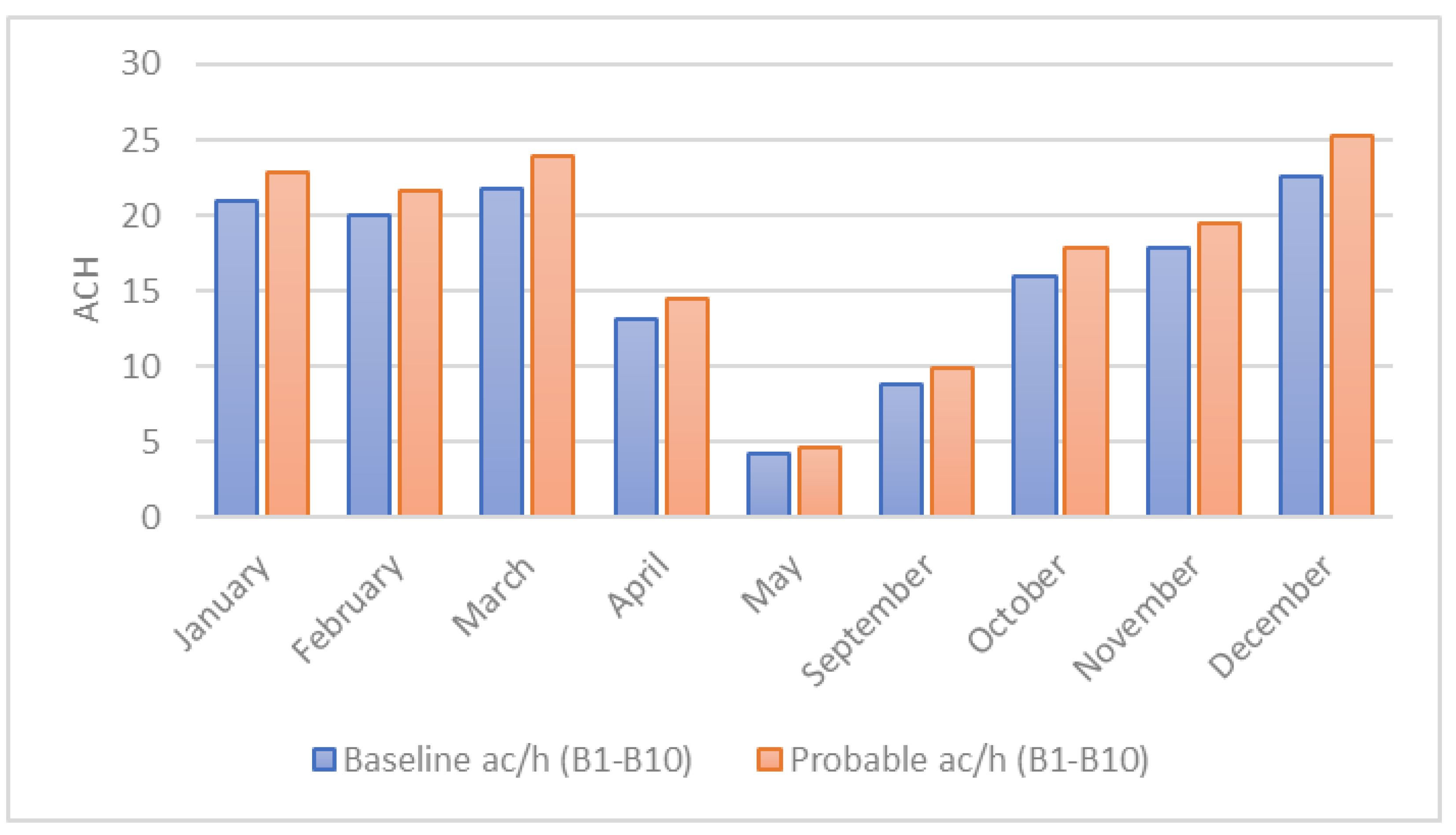
North-facing dual-window configurations demonstrated strong NV performance, particularly when window height was maximised. As shown in Table 4, the tallest configuration (Config. 1) achieved a peak rate of 4.67 ACH in March and an annual average of 3.47 ACH, outperforming the shortest configuration by up to 17%. The PB model, which reflects adaptive user patterns such as morning and evening ventilation, further improved monthly ACH by 8.7% to 12.7% over the SB model, particularly during transitional months like March and May (Figure 3). Across all configurations, PB increased monthly ventilation by approximately 10% on average, with peak gains reaching nearly 13%. These results underscore the value of aligning window design with actual occupant routines rather than relying on static operation assumptions. The findings confirm that occupant interaction plays a pivotal role in achieving optimal NV, even when geometric configurations are already favourable.
However, greater window height and width also resulted in increased solar gains, advantageous in cooler months but potentially problematic during summer. For instance, solar heat gains were substantial in spring (exceeding 400 kWh in March and May), indicating that without shading, large north windows could cause overheating. Although solar exposure was not directly modelled as an input to occupant behaviour, the correlation between elevated internal heat and increased window operation suggests that users instinctively respond to thermal cues. To optimise year-round performance, it is recommended that shading devices or dynamic glazing be integrated into designs featuring large north-facing windows. This approach balances passive solar benefits with the need to avoid overheating during warmer periods.
Solar gain in Scenario A was also substantial, with peak monthly values exceeding 400 kWh, particularly in configurations with taller or wider glazing (Table 5). Although solar gain was not explicitly modelled as a behavioural input, it likely influenced window use, especially during cooler months when passive heating is desirable. Notably, in warmer months such as February, higher solar exposure coincided with increased ventilation rates, indicating that heat buildup may have prompted occupants to open windows for thermal comfort. These observations highlight the dual function of north-facing windows in supporting both passive heating and ventilation. To prevent overheating in summer while preserving these benefits, the use of external shading or low-SHGC glazing is strongly recommended.
3.1.2. Scenario B: 4.5 m × 2.6 m
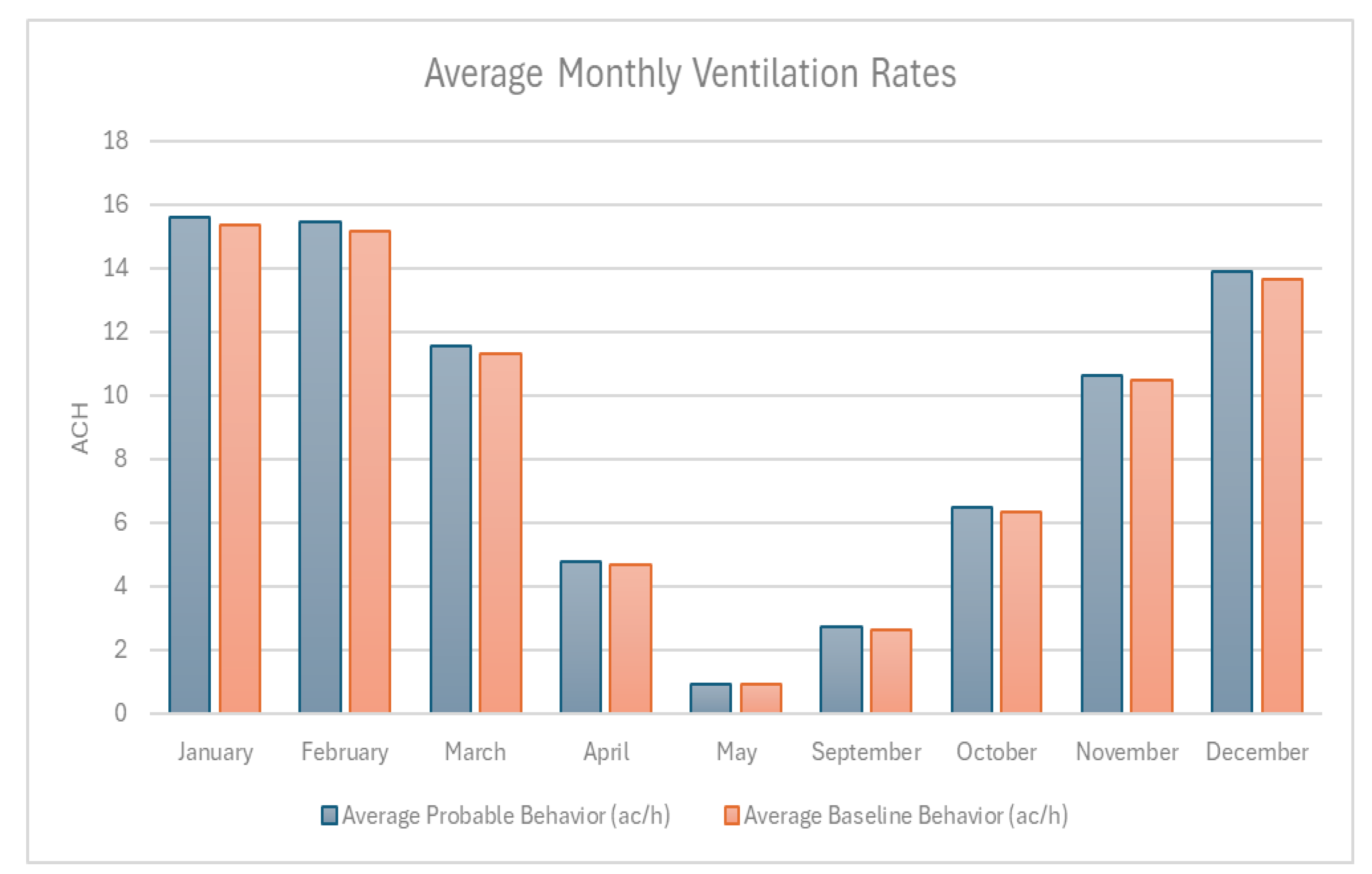
Scenario B applied the same north-facing orientation and 45% WWR to a shorter 4.5 m wall, with proportionally scaled window dimensions. NV performance followed a similar seasonal pattern to Scenario A, peaking in late summer, particularly February, when prevailing winds were more favourable, and declining sharply into late autumn. As shown in Table 6, Configuration 9 achieved the highest peak ventilation rate of 2.86 ACH in February and the highest average of 2.09 ACH across the year, while Configuration 12 recorded the lowest performance with a peak of 2.44 ACH and an average of 1.84 ACH. These results confirm that taller window configurations continued to outperform shorter ones even on smaller wall areas, although the overall ventilation potential was lower than in Scenario A due to reduced façade dimensions. Complete window closure in the coldest winter months further constrained NV performance, reinforcing the need to balance spatial constraints with design elements that support airflow under varying seasonal conditions.
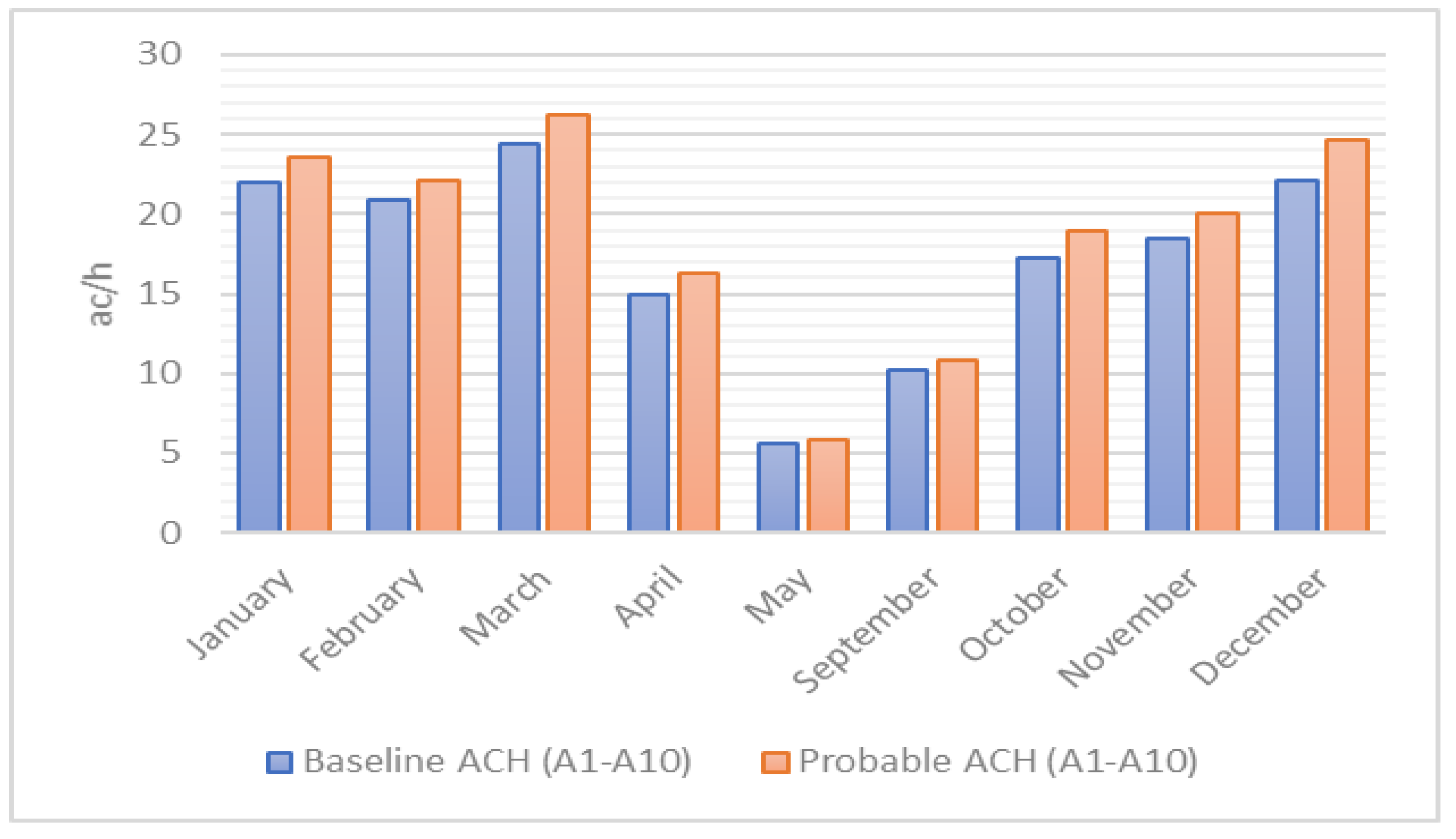
Figure 4 further illustrates the average monthly ventilation rates for Scenario B under both BS and PB models. The figure highlights a consistent uplift in ventilation performance when occupant variability is considered. Across all months, PB yields higher ACH values than the BS, with the most pronounced gains observed during transitional months like May, September, and October, ranging from approximately 8% to 12%. In summer months (January–March), the difference between PB and SB narrows, suggesting that even baseline patterns align reasonably well with environmental drivers. However, during shoulder seasons, occupants under PB adapt window use more responsively to temperature and airflow cues, enhancing NV effectiveness. These results reinforce the importance of integrating adaptive behavior into window design strategies, particularly in spatially constrained layouts like Scenario B.
Table 7 compares the monthly performance of NV and solar gain for Design Story 1, Scenario B, under BS and PB models. Configuration 9 consistently achieved the highest NV rates, while Configuration 12 remained the lowest performer. The PB model led to steady gains in ventilation across all months, with average increases ranging from 5.1% in May to 10.6% in January, particularly notable during warmer and transitional months like February (+10.3%) and December (+9.0%). Although solar gains were moderate due to smaller glazing areas, they peaked at nearly 272 kWh in May (Config. 15) and aligned with higher ventilation activity during warmer months, suggesting that internal heat build-up prompted increased window operation. These results highlight the importance of accounting for both adaptive occupant behavior and passive solar exposure, especially in compact wall designs where spatial constraints limit airflow potential.
Solar gain in Scenario B, while lower than those in Scenario A due to reduced total glazing area, remained significant, ranging from 148 kWh in January to a peak of nearly 272 kWh in May. These values, though modest, are sufficient to influence indoor thermal conditions during transitional seasons and likely contributed to increased ventilation activity under the PB model. As shown in Table 7, months with higher solar gain, such as February and March, coincided with elevated NV rates, reinforcing the hypothesis that internal heat accumulation encourages occupants to open windows for cooling. Configuration 15 consistently exhibited the highest solar gains across all months, reflecting the role of window dimensions in modulating passive heat entry. This finding highlights the dual influence of geometry and adaptive behavior in shaping NV outcomes. To enhance thermal comfort without compromising airflow, especially during warmer periods, the integration of external shading or advanced glazing strategies should be considered in future adaptive design solutions.
3.1.3. Discussion: Design Implications and Behavioral Insights
Larger north-facing windows clearly improved ventilation, but effective passive design also required occupant-responsive use and shading to avoid overheating. Scenario A suits cooler contexts needing passive heating, while Scenario B may be better for warmer climates, offering effective NV without excessive solar heat gain.
3.2. Design Story Two-East and Two-West Configuration
Design Story two examines a system with a large east-facing window, 40% WWR, and a smaller west-facing window, 30% WWR, on opposing walls. This design story aims to promote NV and support occupant comfort throughout the day. A large east-facing window, extending to the ceiling, captures early daylight and warmth, while a smaller west-facing window supports cross-ventilation in the afternoon. The configuration is tailored to Melbourne’s climate, where mornings are often cool and breezy, and afternoons can become warm and still. Occupant behavior in this scenario involves using the east window actively in the morning and gradually shifting to the west-facing opening later in the day, with both windows opened fully in the evening to maximize cross-ventilation. Nine configurations were tested for both Scenarios A and B, each varying in window dimensions to assess their impact on ventilation performance and occupant interaction.
3.2.1. Scenario A: 7 m × 2.6 m East and West Walls
The NV rates across configurations show seasonal fluctuations, peaking in summer due to stronger winds, warmer temperatures, and increased occupant tendency to open windows, and dipping in late autumn as winds weaken and temperatures cool. Scenario A consistently exhibited strong ventilation performance, with peak average NV occurring in January and the lowest rates in May, when outdoor conditions were less favorable. This seasonal dip also aligns with occupant reluctance to open windows during colder periods.
Configurations with wider east-facing windows and balanced west-facing openings consistently outperformed others, highlighting the critical role of window sizing and placement in promoting cross-ventilation. Configuration 5 recorded the highest NV rates, while Configuration 6 had the lowest. Wider east-facing windows proved effective in capturing morning inflow, while balanced west openings enhanced afternoon exhaust. Configurations with smaller west-facing windows performed less effectively, particularly in cooler months.
Probable occupant behavior modeled to reflect daily routines and adaptive use of the window resulted in consistent, albeit modest, improvements in NV across all months.

Table 9.
Ventilation and Solar Gain Across Configurations (Scenario A).
| Month | Highest NV (ACH) (Config.) | Lowest NV (ACH) (Config.) | Avg. NV Baseline (ACH) | Avg. NV Probable (ACH) | % Change | Avg. Solar Gain (kWh) | Peak Solar Gain (kWh) (Config.) | Lowest Solar Gain (kWh) (Config.) |
|---|---|---|---|---|---|---|---|---|
| Jan | 27.22 (5) | 25.40 (6) | 26.53 | 26.94 | +1.5% | 675.85 | 692.78 (5) | 651.07 (6) |
| Feb | 27.08 (5) | 25.27 (6) | 26.37 | 26.62 | +0.9% | 588.15 | 602.76 (5) | 567.72 (6) |
| Mar | 19.90 (5) | 18.44 (6) | 19.30 | 19.65 | +1.8% | 502.96 | 515.37 (5) | 484.88 (6) |
| Apr | 8.29 (3) | 7.83 (6) | 8.16 | 8.36 | +2.5% | 324.56 | 332.28 (5) | 313.24 (6) |
| May | 1.80 (5) | 1.65 (6) | 1.76 | 1.83 | +4.0% | 252.71 | 259.14 (5) | 243.35 (6) |
| Sep | 4.75 (3) | 4.35 (6) | 4.64 | 4.70 | +1.3% | 426.45 | 437.02 (5) | 412.11 (6) |
| Oct | 11.34 (5) | 10.60 (6) | 11.05 | 11.22 | +1.5% | 531.93 | 543.68 (5) | 514.41 (6) |
| Nov | 19.00 (5) | 17.90 (6) | 18.63 | 18.85 | +1.2% | 624.50 | 638.66 (5) | 603.80 (6) |
| Dec | 24.93 (5) | 23.05 (6) | 24.11 | 24.51 | +1.7% | 691.49 | 707.88 (5) | 667.50 (6) |
Solar gain also followed a seasonal trend, with the highest values recorded in summer. In December, Configuration 5 reached a peak of 707.88 kWh, largely due to its large glazed east-facing surface and favorable morning solar angles. High solar gain was also observed in January and February, with levels exceeding 690 kWh across several configurations. These conditions support passive heating during cooler months but may increase thermal load in summer if not mitigated through shading or occupant action. Notably, increased solar gain in February aligned with higher NV rates, suggesting a behavioral response, occupants opening windows more to counteract heat buildup.
The results analysis reinforces the significance of east–west window arrangements, which, when aligned with Melbourne’s wind and sun patterns, can deliver high levels of ventilation and solar access year-round. The influence of window size, orientation, and user interaction is evident in both airflow and thermal outcomes, highlighting the importance of integrating architectural and behavioral strategies in passive design. In overall, the table illustrates how east–west window arrangements can support high levels of both ventilation and solar gain, with design details (e.g., window sizing and placement) and occupant behavior both playing critical roles in optimizing performance.
3.2.2. Scenario B: 4.5 m × 2.6 m East and West Walls
Scenario B follows the same design and behavioral logic on a smaller wall, and while total airflow rates were naturally lower due to reduced window area, the seasonal patterns and behavioral responsiveness mirrored Scenario A. Peak ventilation again occurred in January (15.35 ACH), with the lowest average in May (0.91 ACH).
Table 10.
Natural Ventilation Performance of East–West Windows (Scenario B).
| Configuration | Peak (ACH) (Month) | Lowest (ACH) (Month) | Average (ACH) (Sep–May) |
|---|---|---|---|
| 1 | 15.52 (January) | 0.90 (May) | 7.90 |
| 2 | 15.55 (January) | 0.91 (May) | 7.96 |
| 3 | 15.71 (January) | 0.93 (May) | 8.07 |
| 4 | 15.40 (January) | 0.90 (May) | 7.87 |
| 5 | 15.45 (January) | 0.92 (May) | 7.87 |
| 6 | 15.26 (January) | 0.91 (May) | 7.80 |
| 7 | 15.21 (January) | 0.90 (May) | 7.74 |
| 8 | 14.87 (January) | 0.89 (May) | 7.60 |
| 9 | 15.18 (January) | 0.90 (May) | 7.73 |
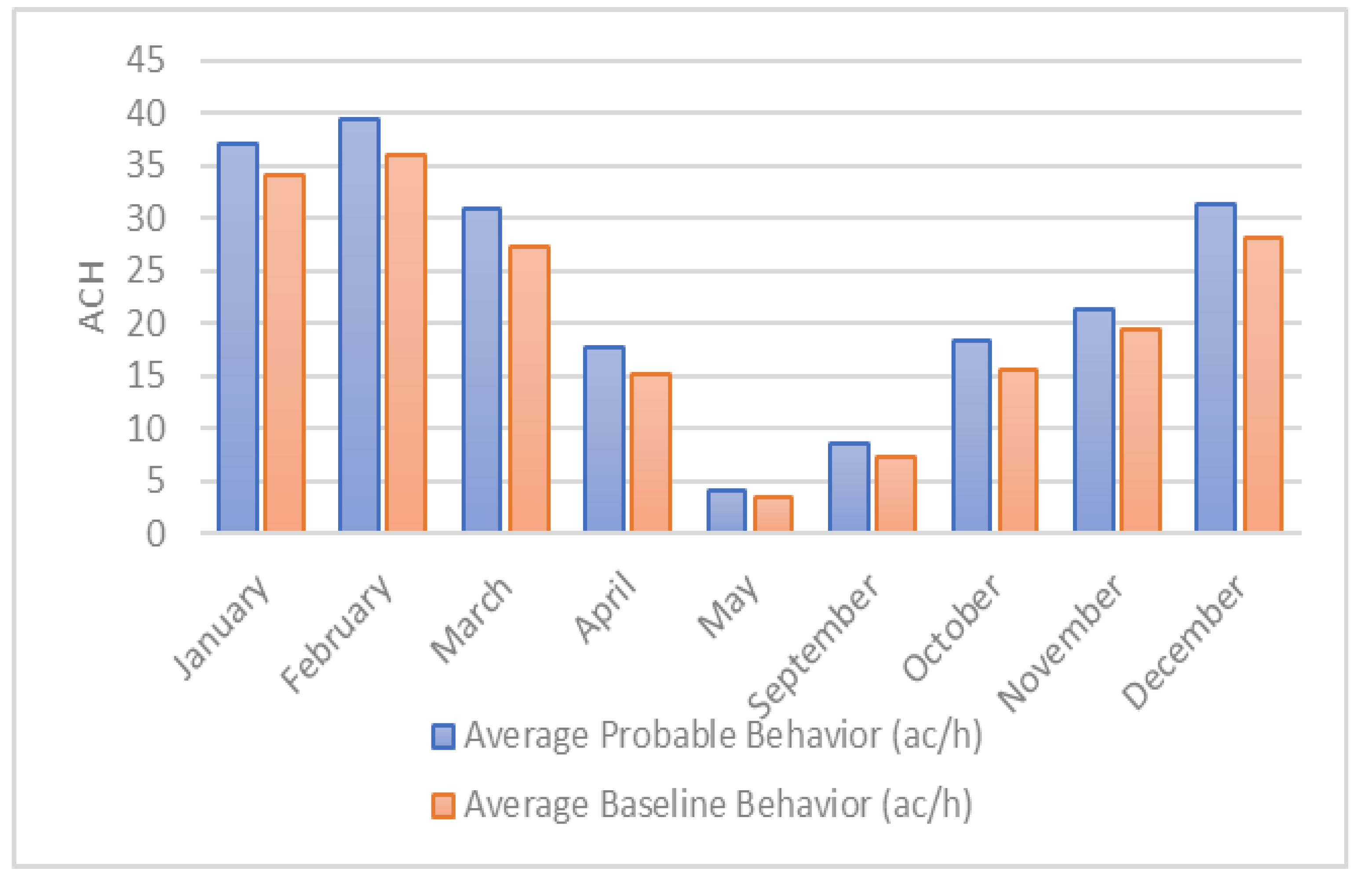
The behavior-adjusted gains ranged from +1.4% to +3.3%, with the largest improvement in May, as seen in figure six.This scenario reinforces the idea that occupant behavior can make a subtle but consistent difference particularly during marginal weather months, where windows might otherwise remain closed or be used less efficiently. The design's responsiveness to behavior is especially visible in the transitional seasons (April, September, October), where increased use of the west window in the afternoon helped extend ventilation into the evening.
Figure 6.
Natural Ventilation Rates Across Configurations - Baseline Behavior (Scenario B).
Solar gain values were naturally lower in Scenario B due to smaller window areas, but still substantial, reaching 438.28 kWh in December. These levels are sufficient to influence thermal comfort and occupant decisions around window usage or shading devices, highlighting the link between passive solar exposure and user behavior.
Table 11.
Ventilation and Solar Gain Under SB and PB Models (Scenario B).
| Month | Highest NV Probable (ACH) (Config.) | Lowest NV Probable (ACH) (Config.) | Avg. NV Baseline (ACH) | Avg. NV Probable (ACH) | % Change | Avg. Solar Gain (kWh) | Peak Solar Gain (kWh) (Config.) | Lowest Solar Gain (kWh) (Config.) |
|---|---|---|---|---|---|---|---|---|
| Jan | 15.71 (3) | 14.87 (8) | 15.35 | 15.62 | +1.8% | 421.33 | 428.61 (3) | 411.11 (8) |
| Feb | 15.49 (3) | 14.65 (8) | 15.14 | 15.45 | +2.0% | 367.55 | 373.29 (3) | 358.56 (8) |
| Mar | 11.64 (3) | 11.04 (8) | 11.31 | 11.54 | +2.0% | 313.62 | 318.93 (3) | 306.37 (8) |
| Apr | 4.84 (3) | 4.52 (8) | 4.67 | 4.79 | +2.6% | 202.74 | 206.07 (3) | 198.15 (8) |
| May | 0.93 (3) | 0.89 (8) | 0.91 | 0.94 | +3.3% | 157.65 | 160.58 (3) | 153.94 (8) |
| Sep | 2.72 (5) | 2.55 (9) | 2.64 | 2.71 | +2.7% | 266.40 | 270.89 (3) | 260.51 (8) |
| Oct | 6.50 (3) | 6.12 (8) | 6.33 | 6.47 | +2.2% | 332.32 | 337.49 (3) | 325.42 (8) |
| Nov | 10.78 (3) | 10.14 (8) | 10.49 | 10.64 | +1.4% | 389.68 | 395.90 (3) | 381.66 (8) |
| Dec | 14.06 (3) | 13.18 (8) | 13.64 | 13.89 | +1.8% | 431.23 | 438.28 (3) | 421.61 (8) |
3.1.3. Discussion: Design Implications and Behavioral Insights
Design Story Two underscores the value of east-west window configurations for effective cross-ventilation, leveraging larger east-facing windows to harness morning breezes and smaller west-facing windows for afternoon airflow. Scenario A’s larger walls boost ventilation, making it well-suited for temperate climates with diurnal wind patterns, while Scenario B’s compact layout fits space-limited settings. Occupant adaptability, enabled by strategic window sizing, enhances natural ventilation (NV) and thermal comfort by aligning with daily wind cycles.
The configuration’s strength lies in its synergy with natural occupant routines, favoring east windows in the morning and west windows later in the day. This demonstrates that windows should be purposefully placed and proportioned to complement how people live, not just maximize size. By encouraging proactive window use, this design improves ventilation efficiency and strengthens occupants’ connection to their surroundings, a cornerstone of human-centered passive design.3.3
Design Story Three: Two South-Facing Windows 45%
Design Story three explores a single-sided ventilation strategy using two south-facing windows with a combined WWR of 45%, ten configurations in Scenario A and nine in Scenario B. The south orientation capitalizes on Melbourne’s consistent diffuse daylight and gentle breezes while minimizing direct solar impact, offering glare-free lighting and thermally stable conditions. For south-facing windows, occupants typically open windows in the morning to capture gentle breezes and diffuse light, adjust openings around midday to manage glare and heat, and reopen them in the evening to facilitate stack-driven exhaust
3.3.2. Scenario A: 7.0m × 2.6 m
NV rates vary seasonally, peaking in summer due to higher temperatures and stronger winds, and declining in late autumn as outdoor conditions cool and wind speeds drop.
Table 12.
Ventilation and Solar Gain - Design Story 2, Scenario B (Baseline and Probable Behaviors).
Table 12.
Ventilation and Solar Gain - Design Story 2, Scenario B (Baseline and Probable Behaviors).
| Story | Peak (ACH) (Month) | Lowest (ACH) (Month) | Average (ACH) |
|---|---|---|---|
| Story 1 | 24.79 (January) | 1.70 (May) | 13.40 |
| Story 2 | 24.76 (January) | 1.69 (May) | 13.38 |
| Story 3 | 24.08 (January) | 1.63 (May) | 12.96 |
| Story 4 | 24.99 (January) | 1.73 (May) | 13.57 |
| Story 5 | 30.07 (January) | 2.27 (May) | 16.67 |
| Story 6 | 23.21 (January) | 1.58 (May) | 12.49 |
| Story 7 | 27.82 (January) | 1.91 (May) | 15.27 |
| Story 8 | 27.60 (January) | 1.94 (May) | 15.17 |
| Story 9 | 21.76 (January) | 1.57 (May) | 11.68 |
| Story 10 | 28.18 (January) | 1.91 (May) | 15.42 |
Configurations with taller, evenly sized windows outperform others, leveraging vertical openings to enhance stack-driven airflow. In contrast, narrower or uneven windows yield lower NV rates, especially in cooler months. On average, designs with balanced dimensions consistently perform well. Under the probable behavior model, NV performance improves slightly by +1.1% to +3.2% as occupants respond dynamically to environmental conditions, particularly during morning and evening periods when ventilation is most effective.
Figure 7.
Natural Ventilation Rates Across Configurations - Baseline Behavior (Scenario A).

Solar gain is highest in December and January, with wide and tall windows like Configuration 5, capturing the most heat up to 708.39 kWh in December. This thermal input enhances comfort in winter but may pose overheating risks in summer unless managed through shading devices or reduced opening durations. Notably, higher solar gain often coincides with increased ventilation, suggesting that elevated indoor temperatures may encourage window use for thermal regulation.
Table 13.
Ventilation and Solar Gain - Design Story 3, Scenario A (Baseline and Probable Behaviors).
Table 13.
Ventilation and Solar Gain - Design Story 3, Scenario A (Baseline and Probable Behaviors).
| Month | Highest NV Probable (ACH) (Config.) | Lowest NV Probable (ACH) (Config.) | Avg. NV Baseline (ACH) | Avg. NV Probable (ACH) | % Change | Avg. Solar Gain (kWh) | Peak Solar Gain (kWh) (Config.) | Lowest Solar Gain (kWh) (Config.) |
|---|---|---|---|---|---|---|---|---|
| Jan | 30.07 (5) | 21.76 (9) | 25.75 | 25.70 | -0.2% | 626.69 | 708.39 (5) | 535.21 (9) |
| Feb | 29.64 (5) | 21.46 (9) | 25.20 | 25.22 | +0.1% | 547.62 | 603.69 (5) | 466.66 (9) |
| Mar | 21.86 (5) | 15.92 (9) | 18.61 | 18.89 | +1.5% | 467.46 | 515.69 (5) | 398.63 (9) |
| Apr | 9.62 (5) | 7.00 (9) | 8.16 | 8.18 | +0.2% | 302.59 | 332.61 (5) | 257.57 (9) |
| May | 2.27 (5) | 1.57 (9) | 1.79 | 1.78 | -0.6% | 233.97 | 259.52 (5) | 199.95 (9) |
| Sep | 5.47 (5) | 3.87 (9) | 4.64 | 4.56 | -1.7% | 398.31 | 437.60 (5) | 338.82 (9) |
| Oct | 12.84 (5) | 9.20 (9) | 10.98 | 11.00 | +0.2% | 499.50 | 543.92 (5) | 423.22 (9) |
| Nov | 20.99 (5) | 14.89 (9) | 17.82 | 17.66 | -0.9% | 585.16 | 638.89 (5) | 496.55 (9) |
| Dec | 27.36 (5) | 19.46 (9) | 23.27 | 23.36 | +0.4% | 645.04 | 708.39 (5) | 548.90 (9) |
Scenario A’s symmetrical layout promotes balanced airflow and spatial comfort. Occupants engage more actively with both windows during midday and early afternoon, especially when external conditions support comfortable indoor temperatures.
Although some months e.g., January, May, September, November, show slightly lower NV values under probable behavior , these variations reflect nuanced behavioral responses such as shorter opening durations due to thermal comfort, noise, or privacy concerns rather than design inefficiencies.
3.3.2. Scenario B: 4.5 m × 2.6 m
Scenario B used the same two south-facing windows but on a shorter 4.5-meter wall, maintaining a 45% WWR. The smaller wall area gave the windows a more prominent presence in the space and subtly shifted the way air moved indoors. As expected, overall ventilation was lower compared to Scenario A due to the limited wall surface, with airflow peaking around 13.11 air changes per hour (ACH) in January and dropping to just 0.79 ACH in May see Table 14.
Despite the lower ventilation potential, occupant behavior still played a meaningful role. When likely behaviors were factored in such as opening windows at certain times of day or in response to comfort needs modest improvements were seen, especially during mild months like May and October. These months showed relative gains of +0.8% to +2.9% compared to baseline, suggesting people are more inclined to open windows when temperatures are comfortable and indoor comfort can be fine-tuned naturally.
In some months, however, the model showed slight decreases in ventilation under probable behavior.These drops don't suggest a flaw in the design, but rather reflect realistic tendencies, people don’t always open windows when models assume they would. They might delay it until the room feels warm enough or avoid it due to noise, wind, or privacy concerns. These subtleties highlight how important it is to design for actual behavior, not just theoretical use.
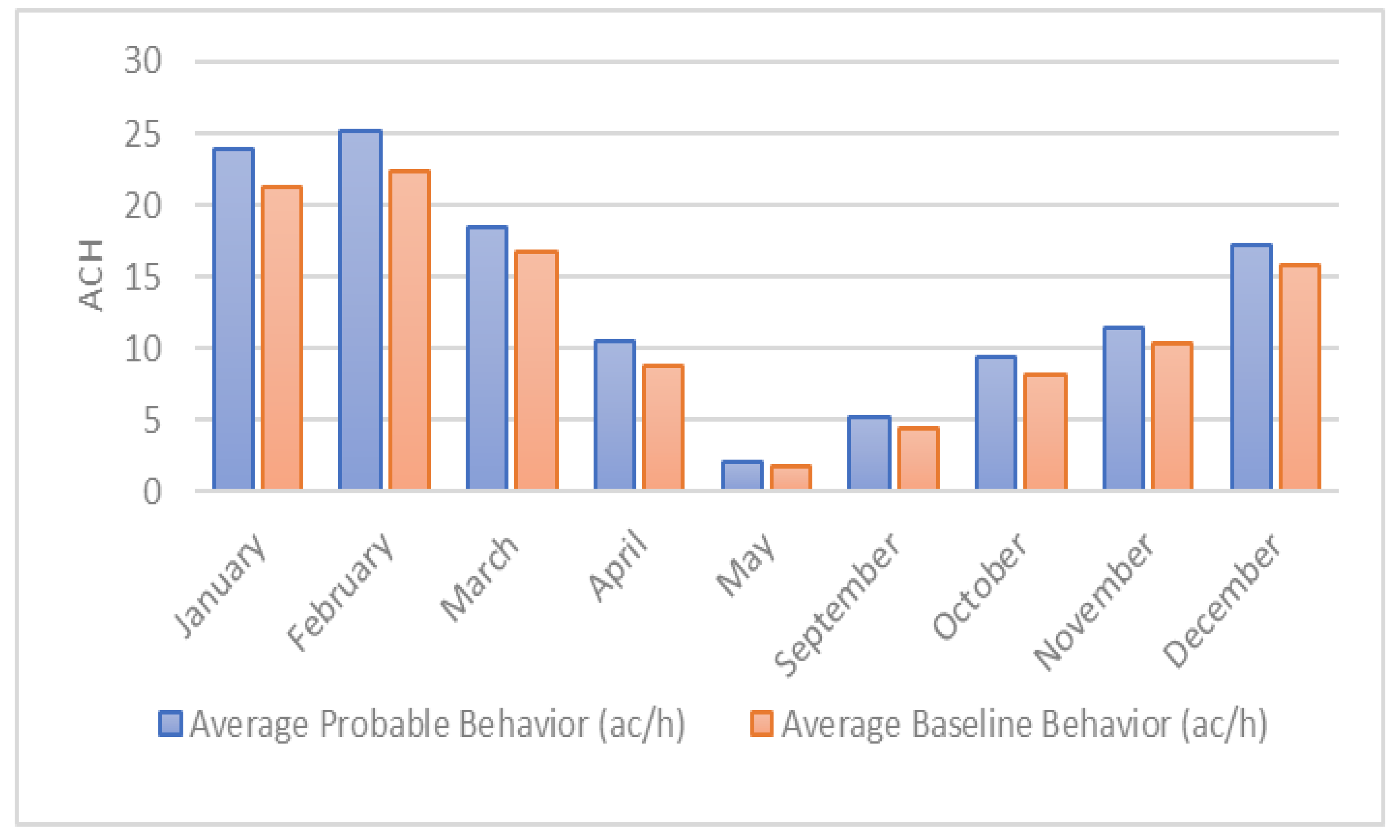
Figure 8.
Story 3, Scenario B - Average Monthly Ventilation Rates (ACH) - Baseline vs. Probable Behaviors.
Figure 8.
Story 3, Scenario B - Average Monthly Ventilation Rates (ACH) - Baseline vs. Probable Behaviors.
Solar gain also followed a similar pattern. Though overall heat gain was lower than in Scenario A, it was still significant, peaking at around 408.92 kWh in December. Taller window configurations captured more sunlight, especially around midday, helping to passively warm interiors during cooler months. This natural warmth often meant windows were opened later in the day, after indoor temperatures had already risen a subtle but telling sign of how solar gain can shape how and when people engage with their space.
Overall, Scenario B underscores the idea that good design isn’t just about maximizing performance on paper it’s about aligning with how people actually live. Even small shifts in behavior can shape how effectively a space breathes. Designing windows that naturally encourage engagement by being easy to use, well-placed, and responsive to daylight and temperature can make all the difference in how a space feels and functions day to day.
3.3.3. Discussion: Design Implications and Behavioural Insights
One of the standout findings is that symmetry supports user perception of balance and encourages even use of windows, making the act of opening feel intuitive. Furthermore, the alignment with solar paths favoring midday and early afternoon gain means that this configuration can effectively reduce heating needs in winter and still offer good ventilation if overheating is addressed through timing or shading.
This design story offers a practical example of how symmetrical, south-facing windows can serve as both a thermal comfort tool and a behavioral cue. By placing equal openings along a single orientation that receives stable solar exposure, the design encourages occupants to open both windows simultaneously, maximizing perceived and actual airflow. The absence of extreme sun angles unlike east or west windows supports prolonged, low-glare usage ideal for work or relaxation spaces.
From a design perspective, this configuration demonstrates that user-friendly ventilation doesn’t necessarily require dynamic geometry or multi-orientation setups. Instead, it shows how clear, simple design aligned with occupant habits and climate-driven needs can foster better interaction with the building envelope. The south-facing orientation becomes a mediator of light, heat, and airflow, and the behavioral data suggests that when such windows are comfortable to use and visually balanced, occupants are more likely to engage with them throughout the year.
3.4. Design Story Four: North-South Window Configuration
Design Story four examines two north-facing windows , 25% WWR each, and one large south-facing window 40% WWR, on opposing walls. The primary design intent was to optimize cross-ventilation by establishing airflow between opposing walls, while simultaneously taking advantage of diffuse daylight from the north and solar warmth from the south especially beneficial during Melbourne’s cooler seasons.Ten configurations for Scenario A and nine for Scenario B vary window dimensions to assess their impact on ventilation and occupant interaction, with specific dimensions. For north and south windows, occupants are likely to open north-facing windows in the morning to capture fresh air and breezes, adjust midday to manage heat or glare, and increase south-facing window openings in the evening for exhaust, adapting to thermal conditions, glare, and privacy needs.
3.4.1. Scenario A: 7 m × 2.6 m North and South Walls
The NV rates across configurations in Scenario A, display clear seasonal variation. Rates peak in late summer, driven by stronger winds, warmer temperatures, and occupants’ increased tendency to open windows. They drop in late autumn as wind speeds diminish and temperatures cool. Configurations with larger north-facing windows consistently outperform others, highlighting the benefit of increased window area in capturing prevailing winds for cross-ventilation. Table 16 summarizes these monthly ventilation patterns under baseline behavior.
When occupant behavior is adjusted to reflect probable patterns such as prioritizing morning inflow via north-facing windows and evening exhaust through south-facing ones, NV rates improve further. Configurations where occupants make fewer or smaller window adjustments, particularly during midday, tend to show reduced performance. This reflects common behaviors such as managing indoor heat or glare.
Figure 9.
Natural Ventilation Rates Across Configurations - Baseline Behavior (Scenario A).
Solar gain, peaks in February across all configurations. Configurations with wider south-facing windows capture more solar heat, which aligns with increased NV activity in that month. This suggests that higher indoor temperatures may encourage occupants to open windows for cooling, supporting the link between solar gain and adaptive ventilation behavior. This balance can be further optimized with shading devices to modulate thermal comfort without compromising airflow.
Table 17 provides a clear summary of monthly NV and solar gain outcomes for Scenario A under both baseline and probable behavior models. Compared to the baseline, the probable behavior model results in consistent improvements in NV rates across all months, with increases ranging from +7.6% in December to a substantial +21.6% in May.
These improvements suggest that occupants are more inclined to interact with windows when comfort conditions are favorable and window operation feels intuitive and effective.
Overall, the cross-orientation layout of Scenario A supported natural airflow regulation across seasons. The size and vertical placement of the south-facing window encouraged its use during periods of heat buildup, while the dual north-facing windows remained consistently accessible for fresh air intake, especially during milder and humid conditions. The resulting ventilation paths were stable, long, and intuitively activated by occupant behavior, reflecting strong synergy between form and function.
3.4.2. Scenario B: 4.5 m × 2.6 m North and South Walls
In Scenario B, the same window layout was applied to shorter 4.5-meter walls, maintaining the original WWRs but adapting the probable behavior. As observed , ventilation performance decreased somewhat due to the reduced cross-sectional area for airflow. Ventilation peaked in January, while May recorded the lowest rate.
Behaviorally, probable interaction again boosted performance modestly, with relative increases of +0.9% to +3.1%, especially in transition months like October and March, where internal conditions prompted more nuanced occupant decisions.
Figure 10.
Natural Ventilation Rates Across Configurations - Baseline Behavior (Scenario B).
The south-facing window continued to deliver strong solar gains, reaching 474.85 kWh in December, a meaningful figure given the smaller room volume and surface area. This gain improved thermal conditions in winter and shoulder seasons, often leading occupants to delay window opening until later in the afternoon, once internal heat gain had leveled off. This deferred engagement points to a more strategic interaction pattern, where in users modulate ventilation not only for airflow, but also for thermal preservation.
Although airflow capacity was reduced compared to Scenario A, Scenario B retained effective thermal regulation and ventilation bursts, particularly when all three windows were operated in coordination. The slightly compressed spatial dimensions made window timing more critical; short openings had stronger impacts on room conditions due to the smaller volume, and users appeared to adjust accordingly.
Table 19.
Highest and Lowest Ventilation Performers by Month for Probable Behavior (Scenario B).
| Month | Highest NV (ACH) (Config.) | Lowest NV (ACH) (Config.) | Avg. NV Baseline (ACH) | Avg. NV Probable (ACH) | % Change | Avg. Solar Gain (kWh) | Peak Solar Gain (kWh) (Config.) | Lowest Solar Gain (kWh) (Config.) |
|---|---|---|---|---|---|---|---|---|
| Jan | 22.42 (6) | 19.65 (5) | 21.23 | 23.86 | +12.4% | 269.77 | 280.93 (6) | 263.57 (1) |
| Feb | 23.75 (6) | 20.87 (5) | 22.36 | 25.18 | +12.6% | 268.43 | 277.28 (6) | 261.87 (1) |
| Mar | 17.48 (6) | 15.56 (5) | 16.67 | 18.43 | +10.6% | 346.27 | 356.11 (6) | 338.75 (1) |
| Apr | 9.13 (6) | 8.52 (10) | 8.78 | 10.52 | +19.8% | 326.68 | 333.73 (6) | 318.47 (1) |
| May | 1.87 (1) | 1.60 (5) | 1.72 | 2.05 | +19.2% | 338.21 | 344.38 (6) | 329.53 (1) |
| Sep | 4.58 (6) | 4.31 (5) | 4.48 | 5.22 | +16.5% | 337.44 | 345.46 (6) | 329.07 (1) |
| Oct | 8.41 (6) | 7.76 (5) | 8.12 | 9.48 | +16.7% | 309.82 | 318.88 (6) | 302.05 (1) |
| Nov | 10.96 (6) | 9.75 (5) | 10.36 | 11.41 | +10.1% | 266.79 | 277.31 (6) | 260.43 (1) |
| Dec | 16.63 (6) | 14.91 (5) | 15.74 | 17.21 | +9.3% | 274.85 | 287.18 (6) | 268.53 (1) |
3.4.2.4. Discussion: Design Implications and Behavioral Insights
Design Story Four illustrates how cross-ventilation can be effectively achieved through thoughtful window placement on opposing walls. The combination of two north-facing windows and one larger south-facing window created a natural airflow loop that aligned with daily occupant routines—inviting cool air in the morning and exhausting warm air in the evening. This intuitive setup encouraged more frequent window use and improved overall ventilation, particularly in larger rooms.
Scenario A, with its longer walls, better supported airflow and daylighting, while Scenario B demonstrated that the same configuration could still work in smaller spaces, though with slightly reduced effectiveness. Occupant behavior played a key role: when windows were used proactively, comfort improved noticeably. However, if windows were kept closed due to glare or external conditions, the benefits diminished.
Overall, this design highlights the importance of aligning architectural elements with natural patterns and occupant habits. By supporting easy and meaningful interaction, the window configuration promoted both thermal comfort and energy-efficient performance without relying on complex systems
3.5. Design Story 5: North-East Window Configuration
Design Story 5 examines a system with one north-facing window with 40% WWR, and two east-facing windows with 25% WWR each. The north and east orientation leverages Melbourne’s morning sunlight and prevailing winds to optimize cross-ventilation. Ten configurations for Scenario A and ten for Scenario B vary window dimensions to assess their impact on ventilation and occupant interaction, with specific dimensions. For north-east windows, occupants are likely to open east-facing windows in the morning to capture fresh air and morning sunlight, adjust midday to manage heat or glare, and increase north-facing window openings in the evening for exhaust, adapting to thermal conditions, glare, and privacy needs.
3.5.1. Scenario A: 7 m × 2.6 m North Wall and 4.5 m × 2.6 m East Wall
NV rates in Scenario A exhibit seasonal variation, peaking in late summer when warmer temperatures, stronger winds, and increased occupant window use align to enhance cross-ventilation. In contrast, rates decline in late autumn as outdoor conditions become less favorable. Among the various story configurations, those with wider north-facing windows consistently outperformed others highlighting the role of window size in facilitating effective exhaust in a cross-ventilation strategy.
Table 20.
Natural Ventilation Rates Across Stories - Baseline Behavior (Scenario A).
| Configuration | Peak (ACH) (Month) | Lowest (ACH) (Month) | Average (ACH) |
|---|---|---|---|
| A1 | 23.81 (March) | 5.36 (May) | 16.22 |
| A2 | 25.39 (March) | 5.89 (May) | 17.32 |
| A3 | 23.86 (March) | 5.39 (May) | 16.25 |
| A4 | 24.09 (March) | 5.38 (May) | 16.37 |
| A5 | 23.66 (March) | 5.30 (May) | 15.95 |
| A6 | 24.08 (March) | 5.38 (May) | 16.29 |
| A7 | 23.73 (March) | 5.38 (May) | 16.07 |
| A8 | 25.18 (March) | 5.87 (May) | 16.92 |
| A9 | 24.06 (March) | 5.43 (May) | 16.24 |
| A10 | 24.73 (March) | 5.82 (May) | 16.58 |
In Scenario A, where the layout prioritizes a wider north-facing façade and a narrower east-facing one, NV consistently performs well, particularly during the warmer months. March stands out with the highest average NV rate of 26.18 ACH under the "probable" occupant behavior model, a significant improvement from the baseline 24.36 ACH, marking a 7.5% increase. This trend is not isolated, other months like January and December also show notable gains of 7.1% and 11.1%, respectively, when occupants actively respond to their environment by opening windows at optimal times. Configuration 2 consistently yields the highest NV rates, peaking at 25.39 ACH in March, while Configuration 5 tends to underperform, showing the lowest values across most months. The data reinforces the effectiveness of a well-sized north-facing window acting as a strong exhaust pathway, especially when paired with strategic east-facing intake openings.
Figure 11.
Story 5, Scenario A - Average Monthly Ventilation Rates (ACH) - Baseline vs. Probable Behaviors.
Figure 11.
Story 5, Scenario A - Average Monthly Ventilation Rates (ACH) - Baseline vs. Probable Behaviors.
In Scenario A, solar gain tends to follow a predictable seasonal rhythm, with the highest values appearing in March. During this month, the average solar gain reached 578.86 kWh, peaking at 605.23 kWh in Configuration 2. This spike can largely be attributed to the larger north-facing windows, which allow more sunlight to pour into the space. As the indoor temperatures rise, it’s natural for occupants to respond by opening windows more frequently, increasing NV to stay comfortable. While this extra sunlight can be beneficial for boosting airflow, it also presents a challenge. Too much solar gain can lead to overheating, especially during peak sun hours. That’s why it's important to consider solutions like shading devices or specially treated glazing to strike a balance between letting in light and maintaining a comfortable indoor environment.
Table 21 compares average NV rates under probable and baseline behaviors. Across all months, probable behaviors improved NV rates by 5.5–11.1%, with the most significant gains observed during transitional seasons like October and December.
3.5.2. Scenario B: 4.5 m × 2.6 m North Wall and 7 m × 2.6 m East Wall
Scenario B, by contrast, reconfigures the orientation; it emphasizes a broader east-facing wall and a more limited north-facing surface. This layout favors early morning ventilation but slightly reduces exhaust potential due to the smaller north window. Despite this, the scenario still performs commendably, particularly when occupant behavior is responsive. December records the highest probable NV rate showing a 12.4% increase, the largest monthly gain across both scenarios. Overall, Scenario B shows a consistently higher behavioral impact on ventilation, with most months posting improvements around 9–12%.
Interestingly, although Scenario B’s ventilation rates are marginally lower than Scenario A’s, its solar gain values are generally higher. This is largely due to the extensive east-facing glazing, which receives strong morning sun. While this can be beneficial for passive heating during winter mornings, it also heightens the risk of overheating in warmer months. Configurations with wider and taller windows consistently register the peak solar gain, indicating the importance of thoughtful sizing and potential need for adjustable shading.
Under the probable behavior model in Scenario B, occupants play a more active role in influencing ventilation outcomes. This model assumes that people respond intuitively to indoor conditions by opening windows during warmer periods or when solar exposure increases. The data shows that this behavior leads to a meaningful increase in NV across the board, with increases ranging from about 8% to over 12%. The highest behavioral impact occurs in December, with a 12.4% improvement in NV, highlighting how even layouts with limited exhaust capacity can still perform well when occupants are engaged. Notably, the consistently higher gains in Scenario B suggest that this configuration is more sensitive to user interaction, meaning thoughtful behavior can significantly offset design limitations.
As for solar gain, Scenario B consistently records higher values than Scenario A, despite its slightly less favorable orientation for NV. This is due to the expansive east-facing glazing that captures intense morning sunlight, especially during the cooler months. For instance, in December, Scenario B achieves an average solar gain of 582.15 kWh, substantially higher than Scenario A’s 493.05 kWh.
Figure 12.
Story 5, Scenario B - Average Monthly Ventilation Rates (ACH) - Baseline vs. Probable Behaviors.
Figure 12.
Story 5, Scenario B - Average Monthly Ventilation Rates (ACH) - Baseline vs. Probable Behaviors.
Configuration 1 frequently records the highest gains, indicating that wider, taller windows facing east are particularly influential in heat accumulation. While this can be beneficial for passive warming in winter, it poses a risk of overheating during warmer months. These findings underscore the importance of integrating adaptable shading or selective glazing into the design, particularly in east-facing zones, to ensure comfort throughout the year.
Table 23.
Ventilation and Solar Gain - Design Story 5, Scenario B (Baseline and Probable Behaviors).
Table 23.
Ventilation and Solar Gain - Design Story 5, Scenario B (Baseline and Probable Behaviors).
| Month | Highest NV Probable (ACH) (Config.) | Lowest NV Probable (ACH) (Config.) | Avg. NV Baseline (ACH) | Avg. NV Probable (ACH) | % Change | Avg. Solar Gain (kWh) | Peak Solar Gain (kWh) (Config.) | Lowest Solar Gain (kWh) (Config.) |
|---|---|---|---|---|---|---|---|---|
| Jan | 21.32 (5) | 20.34 (7) | 20.89 | 22.80 | +9.1% | 555.42 | 564.86 (1) | 548.82 (9) |
| Feb | 20.42 (3) | 19.66 (7) | 20.02 | 21.61 | +8.0% | 532.91 | 541.37 (1) | 526.73 (9) |
| Mar | 21.87 (3) | 21.43 (7) | 21.70 | 23.91 | +10.2% | 552.50 | 559.62 (1) | 546.51 (9) |
| Apr | 13.22 (3) | 12.87 (7) | 13.09 | 14.52 | +11.0% | 441.47 | 446.34 (1) | 436.76 (9) |
| May | 4.23 (2) | 4.11 (7) | 4.17 | 4.67 | +12.0% | 403.35 | 406.77 (1) | 399.15 (9) |
| Sep | 8.92 (4) | 8.67 (7) | 8.83 | 9.92 | +12.3% | 509.27 | 516.59 (1) | 504.76 (9) |
| Oct | 16.22 (4) | 15.43 (7) | 15.90 | 17.84 | +12.2% | 561.58 | 569.92 (1) | 555.23 (9) |
| Nov | 18.09 (3) | 17.55 (7) | 17.81 | 19.53 | +9.7% | 564.13 | 573.79 (1) | 557.46 (9) |
| Dec | 22.99 (3) | 22.06 (9) | 22.52 | 25.31 | +12.4% | 582.15 | 592.25 (1) | 574.96 (9) |
3.5.3. Discussion: Design Implications and Behavioral Insights
In comparing both scenarios, it becomes clear that Scenario A slightly outperforms Scenario B in terms of raw ventilation potential, with a peak of 25.39 ACH versus 22.99 ACH. This advantage is attributed to the wider north-facing window acting as a superior exhaust outlet. However, Scenario B demonstrates a stronger relative response to behavioral changes, suggesting that occupant engagement, such as adjusting windows during specific times, can substantially enhance performance, even when the layout is less inherently optimal. The broader implication is that design alone doesn’t dictate performance; the combination of window orientation, sizing, and occupant behavior collectively determines indoor comfort. Designers should consider not only optimal window configurations but also how adaptable the space is to user interaction. Moreover, to mitigate the risk of excessive solar heat gain while preserving NV, integrating passive design elements like eaves, blinds, or operable shading systems becomes essential, especially in east- and north-facing facades.
In summary, Scenario A offers stronger baseline performance in ventilation and is particularly suited for maximizing daily cross-ventilation, while Scenario B, although slightly weaker in exhaust efficiency, excels in leveraging user behavior and morning solar exposure. Both designs benefit significantly from engaged occupants and show clear seasonal patterns that could inform adaptive strategies year-round.
3.5. Broader Applicability and Transferability
Although the specific numeric results presented here are context-dependent (Melbourne, Australia), the demonstrated relative improvements (5–12% increases in ACH from incorporating occupant behavior) and methodological insights remain valid and transferable. By utilizing the provided workflow, integrating realistic occupant behavior into dynamic simulations, researchers and practitioners globally can achieve similarly optimized results tailored to their local conditions. For example, while in hotter climates, the approach can highlight necessary shading strategies or window operation schedules during peak solar gains, in colder climates, adaptive window configurations could optimize passive solar heating and ventilation trade-offs. Thus, the methodology and core insights have global relevance and can be widely implemented, informing both practical design guidelines and policy recommendations.
3.7. Summary & Guideline
The study highlights that occupant behavior significantly alters window performance outcomes. Simulation results demonstrated considerable differences in ventilation rates and thermal comfort between behavior-informed scenarios and base-case assumptions. Designs that initially appeared optimal under default usage patterns often underperformed when realistic occupant behaviors were introduced. Specifically, in the context of Melbourne's climate, north- and south-facing window designs performed best when aligned with actual occupant use patterns. Large, operable north-facing windows, as seen in Scenarios 1 and 4, enhanced ventilation potential, particularly when placement encouraged interaction. Similarly, high south-facing windows contributed to improved thermal comfort during cooler seasons without introducing excessive overheating risk. Moreover, window placement strongly influenced usability: windows positioned near the ceiling or with restricted access were less likely to be operated, regardless of their ventilation potential, indicating that usability is just as critical as physical performance. Designs with asymmetrical and mixed-orientation windows, such as in Stories 4 and 5, were particularly effective, balancing natural light and airflow while promoting more consistent use throughout the year, especially in transitional seasons. Overall, the findings underscore the necessity for early-stage design processes to integrate realistic occupant behavior models. Relying solely on default assumptions risk overestimating NV performance, whereas behavior-sensitive simulations enable more accurate predictions and support the development of human-centric, high-performing building designs.
Table 24.
Window design recommendations.
| Orientation | Window Design Strategy | Key Parameters | Behavioral Insight | Simulation Outcome | Final Recommendation |
|---|---|---|---|---|---|
| North | Two windows (equal size) | 45% WWR | Frequent opening due to glare-free daylight | High ventilation, low solar gain | ✅ Recommend for daylight + ventilation |
| One large central window | 45% WWR, high placement | Less use due to unreachable height | Medium ventilation, better view | ⚠️ Only if view is priority | |
| South | One large window + two side windows | Total 65% WWR | Overheating during afternoon, limited opening | High solar gain, glare issues | ❌ Not ideal without shading |
| Two medium windows | 45% WWR | Balanced use, easy to open | Moderate ventilation and daylight | ✅ Preferred for comfort | |
| East | Large ceiling height window | 40% WWR | Low opening frequency in morning | Glare issues in early hours | ⚠️ Use only with shading |
| East | Smaller west-facing window | 30% WWR | Opened more in late day | Supports cross ventilation | ✅ Good for morning-evening balance |
| West | One large window | 40% WWR | Often kept shut due to heat | Poor thermal comfort | ❌ Avoid large west-facing glass |
| West | Two smaller splits windows | 45% total WWR | More likely to be opened | Better air flow, lower overheating | ✅ Recommended with shading |
Overall, the guideline table isn’t just a set of random numbers; it’s a thoughtful response to consider Melbourne’s climate. The dimensions are based on simulations that consider local solar angles, wind patterns, and temperature changes, ensuring that homes and buildings maximize energy efficiency and comfort throughout the year. By aligning window sizes and placements with these conditions, the guidelines create practical, climate-responsive designs that work for Melbourne’s residents.
Table 25.
Window design recommendations.
| Orientation | Recommended Window Dimensions | Additional Considerations |
|---|---|---|
| North | - Height: 2.0 m - 2.4 m - Width: 1.5 m - 2.0 m - Aspect ratio (H/W): >1.0 (taller than wide) |
- Place operable part within 1.0-1.5 m from floor for easy access - Total WWR: 40-50% - Ideal for maximizing ventilation and daylight with minimal glare |
| East | - Height: 1.8 m - 2.0 m - Width: 2.0 m - 3.0 m - Aspect ratio: <1.0 (wider than tall) |
- Use shading devices e.g., blinds, overhangs to control morning glare - Suitable for capturing morning light and ventilation |
| West | - Height: 1.5 m - 1.8 m - Width: 1.5 m - 2.0 m - Aspect ratio: ~1.0 (square or slightly rectangular) |
- Use external shading or low-E glass to reduce afternoon heat gain - Smaller windows help manage excessive solar exposure |
| South | - Height: 1.8 m - 2.0 m - Width: 1.8 m - 2.5 m - Aspect ratio: ~1.0 (square or slightly rectangular) |
- Provides consistent daylight without excessive heat gain - Suitable for spaces where glare is less of an issue |
4. Limitations and Future Works
While this study provides valuable insights into optimizing window design for NV by integrating occupant behavior, several limitations should be acknowledged. First, the simulations relied on survey data from Melbourne residents, which may not fully represent behavioral patterns in other climatic or cultural contexts, potentially limiting the generalizability of the findings. Second, the study focused on a single living room model with fixed building characteristics, which may not capture the diversity of residential building typologies or construction materials. Third, the occupant behavior models (same behavior and probable behavior) were based on aggregated survey responses, which may oversimplify the complexity of individual preferences and dynamic interactions with windows, such as responses to real-time environmental feedback or socio-economic factors. Additionally, the study did not account for external factors like urban surroundings (e.g., adjacent buildings or vegetation) that could influence wind patterns and ventilation performance. Future research could address these limitations by expanding the scope to include diverse climatic zones, building types, and occupant demographics to enhance the applicability of the findings. Incorporating real-time occupant feedback through smart sensors or machine learning could refine behavior models, enabling more precise predictions of window use. Additionally, exploring hybrid ventilation systems that combine natural and mechanical strategies could provide practical solutions for challenging urban environments. Finally, integrating multi-objective optimization frameworks, such as cost-benefit analyses or life-cycle assessments, could further evaluate the trade-offs between ventilation performance, energy efficiency, and economic feasibility, supporting practical adoption by architects and builders.
5. Conclusion
This research presented a novel behavior-integrated simulation framework combining occupant behavior models (Same Behavior and Probable Behavior), derived from empirical survey data, with dynamic EnergyPlus simulations to optimize window design for Natural Ventilation in Melbourne’s temperate residential buildings. This research uniquely incorporates realistic occupant behavior, addressing a critical gap often overlooked in conventional simulations. Key numerical findings and insights include:
- Probable Behavior models significantly increased ventilation rates by approximately 5% to over 20% compared to static (Same Behavior) assumptions, highlighting the critical impact of realistic occupant engagement.
- Moderately sized north-facing windows (around 45% WWR) and balanced cross-ventilation designs (e.g., North–South, East–West, North–East) consistently delivered the highest ventilation performance, achieving peak rates around 25–36 ACH in optimal configurations.
- Windows placed within occupant reach (below 1.6 m height) significantly improved usability and thus increased ventilation frequency and effectiveness.
- Large windows placed near ceilings or on west and south orientations resulted in increased solar gain (up to ~700 kWh/month in extreme cases), causing potential overheating and lower window-use frequency.
- Balanced and symmetrical window layouts on the same façade encouraged simultaneous occupant use, enhancing overall ventilation effectiveness.
The study contributes a practical, occupant-sensitive design guideline matrix, enabling architects and engineers to make evidence-based decisions, improving real-world NV performance. While initially tailored to Melbourne’s temperate climate, the occupant-responsive methodology is inherently adaptable; future researchers and practitioners can apply it to other regions by updating climate files, occupant models, and construction standards. Policymakers can also leverage this framework to refine building codes and sustainability policies by aligning them with real-world occupant behavior. Future research directions should explore extending this occupant-integrated approach to different climates, incorporating real-time occupant feedback mechanisms, and integrating advanced adaptive shading and smart ventilation controls for enhanced comfort and energy efficiency.
Acknowledgments
During the preparation of this article, the authors used AI tools to improve readability and language. After using these tools, the authors reviewed and edited the content as needed. They take full responsibility for the content of the publication.
References
- Amasyali, K. , & El-Gohary, N. M. (2018). A review of data-driven building energy consumption prediction studies. Renewable and Sustainable Energy Reviews, 81, 1192-1205.
- Zhan, Sicheng, et al. "Bridging performance gap for existing buildings: The role of calibration and the cascading effect." Building Simulation. Vol. 18. No. 1. Tsinghua University Press, 2025.
- Menezes, A. C. , Cripps, A., Bouchlaghem, D., & Buswell, R. (2012). Predicted vs. actual energy performance of non-domestic buildings. Applied Energy, 97, 355-364.
- de Wilde, P. (2014). The gap between predicted and measured energy performance of buildings: A framework for investigation. Automation in Construction, 41, 40-49.
- van Dronkelaar, C. , Dowson, M., Burman, E., Spataru, C., & Mumovic, D. (2016). A review of the energy performance gap and its underlying causes in non-domestic buildings. Frontiers in Mechanical Engineering, 1, 17.
- Far, Claire, Iftekhar Ahmed, and Jamie Mackee. "Significance of occupant behaviour on the energy performance gap in residential buildings." Architecture 2.2 (2022): 424-433.
- Hong, T. , Taylor-Lange, S. C., D'Oca, S., Yan, D., & Corgnati, S. P. (2016). Advances in research and applications of energy-related occupant behavior in buildings. Energy and Buildings, 116, 694-702.
- Yan, D. , O'Brien, W., Hong. T., Feng, X., Gunay. H. B., Tahmasebi, F., & Mahdavi. A. (2017). Occupant behavior modeling for building performance simulation: Current state and future challenges. Energy and Buildings, 107. 264-278.
- Andersen, R. V., Toftum, J., Andersen, K. K., & Olesen, B. W. (2009). Survey of occupant behavior and control of indoor environment in Danish dwellings. Energy and Buildings, 41(1), 11-16.
- NatHERS Technical Note (Version October 2024) | Nationwide House Energy Rating Scheme (NatHERS). (2019). Nathers.gov.au. https://www.nathers.gov.au/publications/nathers-technical-note.
- Zhang, Yan. "Occupant behavior and its impact on energy consumption of urban residential buildings." (2021).
- Mylonas, Angelos, Aris Tsangrassoulis, and Jordi Pascual. "Modelling occupant behaviour in residential buildings: A systematic literature review." Building and Environment (2024): 111959.
- D'Oca, S. , Chen, C. F., Hong, T., & Belafi, Z. (2017). Synthesizing building physics with social psychology: An interdisciplinary framework for context and occupant behavior in office buildings. Energy Research & Social Science, 34, 240-251.
- Schweiker, M., Fuchs, X., Becker, S., & Wagner, A. (2020). Occupant behavior relation to the connected openings of adjacent spaces in a field study. Building and Environment, 173, 106749.
- O'Brien, W. , & Gunay, H. B. (2014). The contextual factors contributing to occupants' adaptive comfort behaviors in offices: A review and proposed modeling framework. Building and Environment, 77, 77-87.
- Reinhart, C. F. , & Voss, K. (2003). Monitoring manual control of electric lighting and blinds. Lighting Research & Technology, 35(3), 243-260.
- Fabi, V. , Andersen, R. V., Corgnati, S. P., & Olesen, B. W. (2012). Occupants' window opening behaviour: A literature review of factors influencing occupant behaviour and models. Building and Environment, 58, 188-198.
- Haldi, F. Haldi, F., & Robinson, D. (2010). On the unification of thermal perception and adaptive actions. Building and Environment, 45(11), 2440-2457.
- Gunay, H. B., O'Brien, W., & Beausoleil-Morrison, I. (2016). Implementation and comparison of existing occupant behavior models in EnergyPlus. Journal of Building Performance Simulation, 9(6), 567-589.
- Pourtangestani, M. , Izadyar, N., Jamei, E., & Vrcelj, Z. (2024). Linking occupant behavior and window design through post-occupancy evaluation: Enhancing natural ventilation and indoor air quality. Buildings, 14(6), 1638. [CrossRef]
- Arethusa, M. T., Kubota, T., Angung, M., Sri, N., Antaryama, I., & Tomoko, U. (2014). Factors influencing window opening behaviour in apartments of Indonesia. In Proceedings of the 30th International PLEA Conference. Sustainable Habitat for Developing Societies: Choosing the Way Forward (pp. 239-246), Volume 1.
- Chelliah, N. S. , Gnanasambandam, N. S., & Tadepalli, S. (2025). Influence of window design and environmental variables on the window opening behavior of occupants and energy consumption in residential buildings. Transactions on Energy Systems and Engineering Applications, 6(1). [CrossRef]
- ΙΕA. (2021). The role of buildings in the post-COVID recovery. International Energy Agency.
- Rouleau, J. , & Gosselin, L. (2021). Impact of COVID-19 lockdown on building energy consumption and GHG emissions: The case of Québec, Canada. Energy and Buildings, 240, 110924.
- Ferreira, A. , & Barros, N. (2022). COVID-19 and Lockdown: The Potential Impact of Residential Indoor Air Quality on the Health of Teleworkers. International Journal of Environmental Research and Public Health, 19(10), 6079. [CrossRef]
- Heiselberg, P., Svidt, K., & Nielsen, P. V. (2001). Characteristics of airflow from open windows. Building and Environment, 36(7), 859-869.
- Qi, H. , Sha, D., & Zhang, Y. (2020). A review of high-rise ventilation for energy efficiency and safety. Sustainable Cities and Society, 52, 101841.
- Yang, Q. , Liu, M., Shu, C., Mmereki, D., Uzzal Hossain, Md., & Zhan, X. (2015). Impact Analysis of Window-Wall Ratio on Heating and Cooling Energy Consumption of Residential Buildings in Hot Summer and Cold Winter Zone in China. Journal of Engineering, 2015, 1-17.
- Goia, F. (2016). Search for the optimal window-to-wall ratio in office buildings in different European climates and the implications on total energy-saving potential. Solar Energy, 132, 467-495.
- Song, G., Ai, Z., Liu, Z., & Zhang, G. (2022). A systematic literature review on smart and personalized ventilation using CO2 concentration monitoring and control. Energy Reports, 8, 6504-6519.
- Bramiana, C. N. , Aminuddin, A. M. R., Ismail, M. A., Widiastuti, R., & Pramesti, P. L. (2023). The Effect of Window Placement on Natural Ventilation Capability in a Jakarta High-Rise Building Unit. Buildings, 13(5), 1141.
- U.S. Department of Energy. Natural ventilation. Energy Saver https://www.energy.gov/energysaver/natural-ventilation.
- Davenport, A. G. , & Wilson, D. J. (1996). Wind engineering for natural ventilation design. Journal of Wind Engineering and Industrial Aerodynamics, 65(1-3), 1-12.
- Sacht, H., & Lukiantchuki, M. A. (2017). Windows Size and the Performance of Natural Ventilation. Procedia Engineering, 196, 972-979.
- Xu, P. , Shen, Y., & Zhang, X. (2015). Energy performance optimization of windows in hot climates: A parametric study. Energy and Buildings, 103, 15-25.
- Schulze, T., & Eicker, U. (2013). Controlled natural ventilation for energy efficient buildings. Energy and Buildings, 56, 221-232.
- Vanhoutteghem, L., Skarning, G. C. J., Hviid, C. A., & Svendsen, S. (2015). Impact of window design on energy performance in residential buildings. Energy and Buildings, 92, 141-151.
- Roetzel, A. , Tsangrassoulis, A., Dietrich, U., & Busching, S. (2010). On the influence of window design on energy efficiency in different climates. Building and Environment, 45(5), 1263-1275.
- Feng, X., Yan, D., & Wang, C. (2015). Simulation of occupancy in buildings. Energy and Buildings, 87, 348-360.
- D'Oca, S., & Hong, T. (2015). Occupancy schedules learning process through a data mining framework. Energy and Buildings, 88, 395-408.
- Langevin, J. , Wen, J., & Gurian, P. L. (2015). Simulating the human-building interaction: Development and validation of an agent-based model of office occupant behaviors. Building and Environment, 88, 27-45.
- Gaetani, I., Hoes, P. J., & Hensen, J. L. M. (2016). Estimating the influence of occupant behavior on building heating and cooling energy in one simulation run. Applied Energy, 216, 372-383.
- Wang, Y. , Wang, X., & Yu, S. (2023). Understanding the role of occupant behavior in residential building energy consumption: A review of recent advances. Energy and Buildings, 301, 113938.
- Li, C. , Skitmore, M., & He, T. (2022). The post-occupancy dilemma in green-rated buildings: A performance gap analysis. Journal of Green Building, 17(3), 259-278.
- Gram-Hanssen, K. , & Georg, S. (2022). Energy performance gaps: Promises, people, and practices. Buildings and Cities, 3(1), 51-64.
- Rupp, R. F. , Fornari, R. M., & Ghisi, E. (2022). Adaptive thermal comfort models for naturally ventilated buildings: A critical review and future directions. Building and Environment, 218, 109149.
- Wu, Z., Li, N., Wargocki, P., Peng, J., Li, J., & Cui, H. (2019). Adaptive thermal comfort in naturally ventilated dormitory buildings in Changsha, China. Energy and Buildings, 201, 109400.
- Elsayed, M. , Pelsmakers, S., & Pistore, L. (2023). Post-occupancy evaluation in residential buildings: A systematic literature review of current practices in the EU. Building and Environment, 234, 110755.
- Anderson, K., & Lee, S. H. (2016). An empirically grounded model for simulating normative energy use feedback interventions. Applied Energy, 173, 272-282.
- Artan, D. , Ergen, E., Kula, B., & Guven, G. (2022). Rateworkspace: BIM integrated post-occupancy evaluation system for office buildings. Journal of Information Technology in Construction, 27, 441-485. [CrossRef]
- Mylonas, A. , Tsangrassoulis, A., & Pascual, J. (2024). Modelling occupant behaviour in residential buildings: A systematic literature review. Building and Environment, 265, 111959.
- Heiselberg, P., & Bjørn, E. (2002). Experimental investigation of airflow and temperature distribution in a room with natural ventilation. International Journal of Ventilation, 1(1), 55-68.
- Saadi, S. , Hayati, A., & Salmanzadeh, M. (2021). Optimization of Window-to-Wall Ratio for Buildings Located in Different Climates: An IDA-Indoor Climate and Energy Simulation Study. Energies, 14(7), 1974.
- Veillette, D. , Rouleau, J., & Gosselin, L. (2021). Impact of Window-to-Wall Ratio on Heating Demand and Thermal Comfort When Considering a Variety of Occupant Behavior Profiles. Frontiers in Sustainable Cities, 3.
- Ali, D. M. T. E. , Motuzienė, V., & Džiugaitė-Tumėnienė, R. (2023). Al-driven innovations in building energy management systems: A review of potential applications and energy savings. Energies, 17(17), 4277.
- Dai, X. , Liu, J., & Zhang, X. (2020). A review of studies applying machine learning models to predict occupancy and window-opening behaviours in smart buildings. Energy and Buildings, 223, 110159.
- Cao, Q. , Li, X., & Zhang, Y. (2023). Predictive analytics for occupant behavior in smart buildings: A review of machine learning techniques. Building and Environment, 245, 110892.
- Lu, W. , Zhang, L., & Liu, Y. (2024). Evaluation of Urban Complex Utilization Based on AHP and MCDM Analysis: A Case Study of China. Buildings, 14(7), 2179.
- Das, P. , Chalabi, Z., Jones, B., Milner, I., Shrubsole, C., Davies, M., & Wilkinson, P. (2016). Multi-objective methods for determining optimal ventilation rates in dwellings. Building and Environment, 109, 170-181.
- Jiang, Y. , Li, N., Yongga, A., & Yan, W. (2022). Short-term effects of natural view and daylight from windows on thermal perception, health, and energy-saving potential. Building and Environment, 219, 109146.
- Aries, M. B. C. , Aarts, M. P. J., & van Hoof, J. (2015). Daylight and health: A review of the evidence and consequences for the built environment. Lighting Research & Technology, 47(1), 6-27.
- Tomrukcu, G. , & Ashrafian, T. (2024). Climate-resilient building energy efficiency retrofit: Evaluating climate change impacts on residential buildings. Energy and Buildings, 316, 114315.
- Mesloub, A. , Alnaim, M. M., Albagawi, G., Alsolami, B. M., Mahboub, M. S., Tsangrassoulis, A., & Doulos, L. T. (2023). The visual comfort, economic feasibility, and overall energy consumption of tubular daylighting device system configurations in deep plan office buildings in Saudi Arabia. Journal of Building Engineering, 68, 106100.
- Burman, E., Mumovic, D., & Kimpian, J. (2014). Towards measurement and verification of energy performance under the framework of the European directive for energy performance of buildings. Energy, 77, 153-163.
- Delzendeh, E. , Wu, S., Lee, A., & Zhou, Y. (2017). The impact of occupants' behaviours on building energy analysis: A research review. Renewable and Sustainable Energy Reviews, 80, 1061-1071.
- Schmidt, M. , Crawford, R. H., & Warren-Myers, G. (2020). Quantifying Australia's life cycle greenhouse gas emissions for new homes. Energy and Buildings, 190, 1-11. [CrossRef]
- Australian Building Codes Board. (2022). National Construction Code 2022. Canberra: ABCB.
- Dalton, T. (2011). Australian suburban house building: Industry organisation, practices, and constraints. AHURI Posi-tioning Paper No. 143.
- Australian Institute of Refrigeration, Air Conditioning and Heating (AIRAH). (2019). The Australian HVAC&R Industry Guide. Retrieved from https://www.airah.org.
- Climate statistics for Australian locations: Melbourne monthly climate statistics. Retrieved from: http://www.bom.gov.au/climate/averages/tables/cw_086071.
- Xu, X. , Yu, C., & Li, H. (2020). Energy performance of window systems in buildings: A review. Energy and Buildings, 214, 109842.
Figure 1.
Methodological Flowchart.
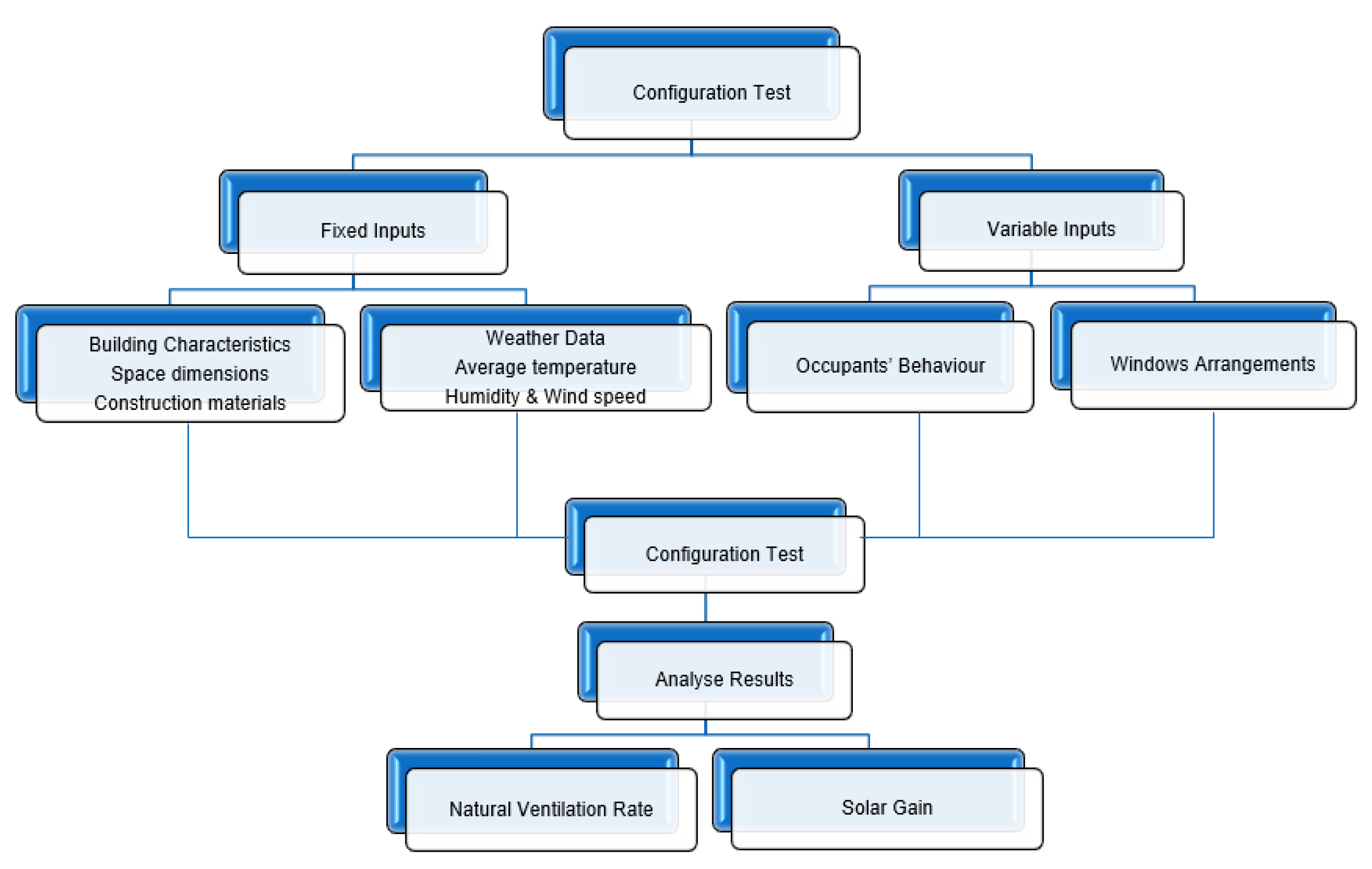
Figure 2.
Design Stories and design scenarios.
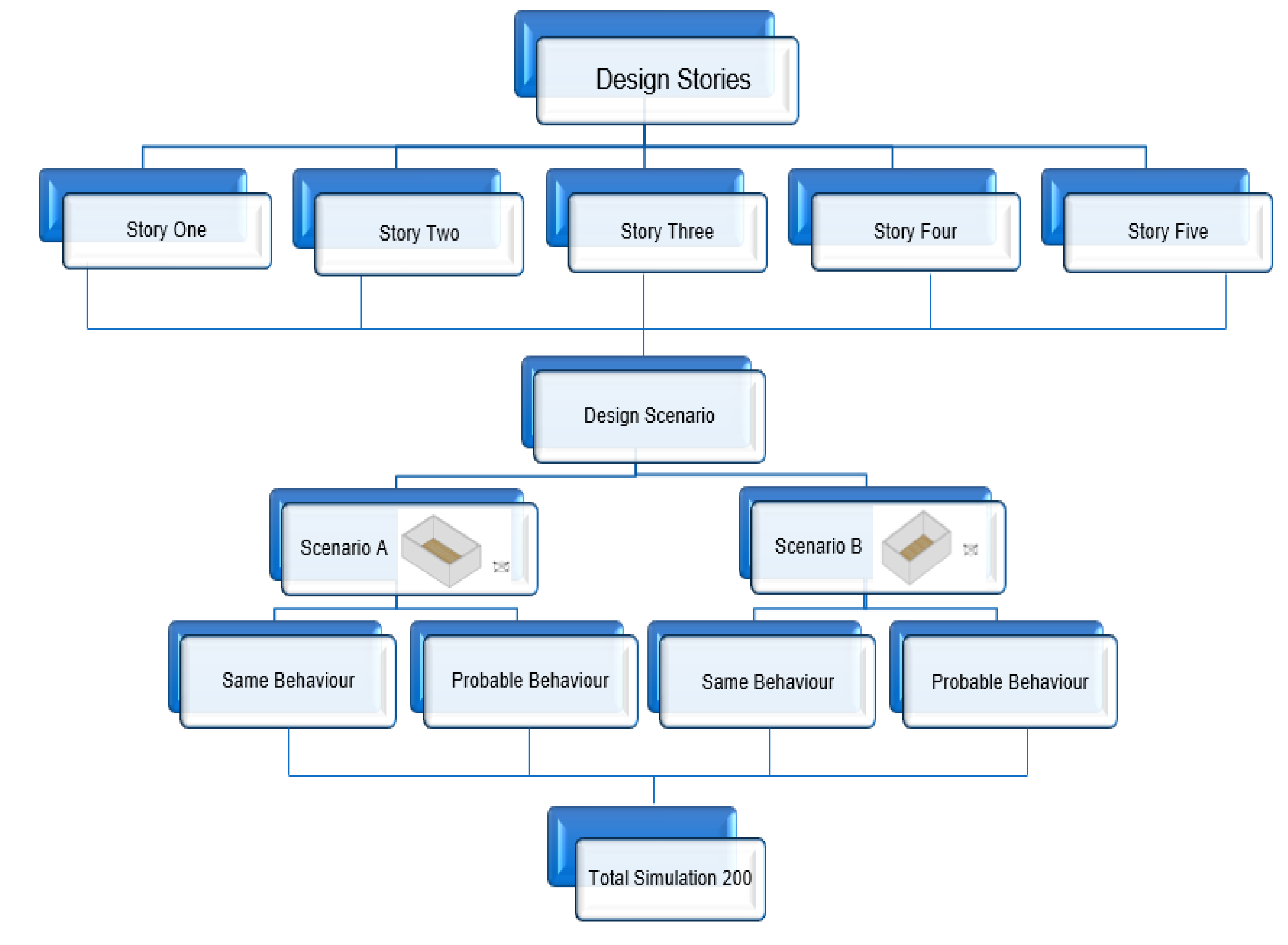
Figure 3.
Story 1, Scenario A - Average Monthly Ventilation Rates (ACH) - Baseline vs. Probable Behaviors.
Figure 3.
Story 1, Scenario A - Average Monthly Ventilation Rates (ACH) - Baseline vs. Probable Behaviors.
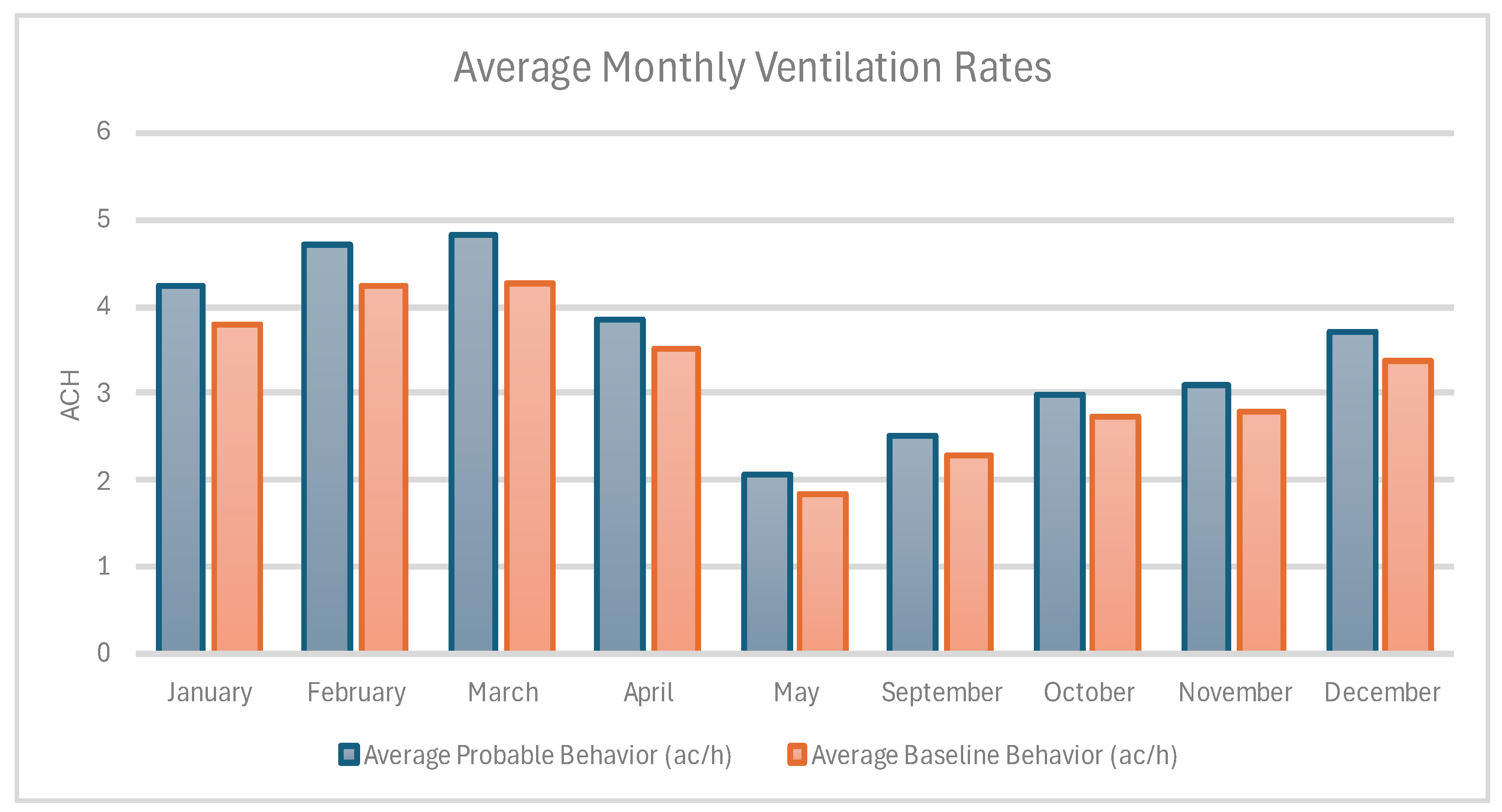
Figure 4.
Natural Ventilation Rates Across Stories - Baseline Behavior (Scenario B).
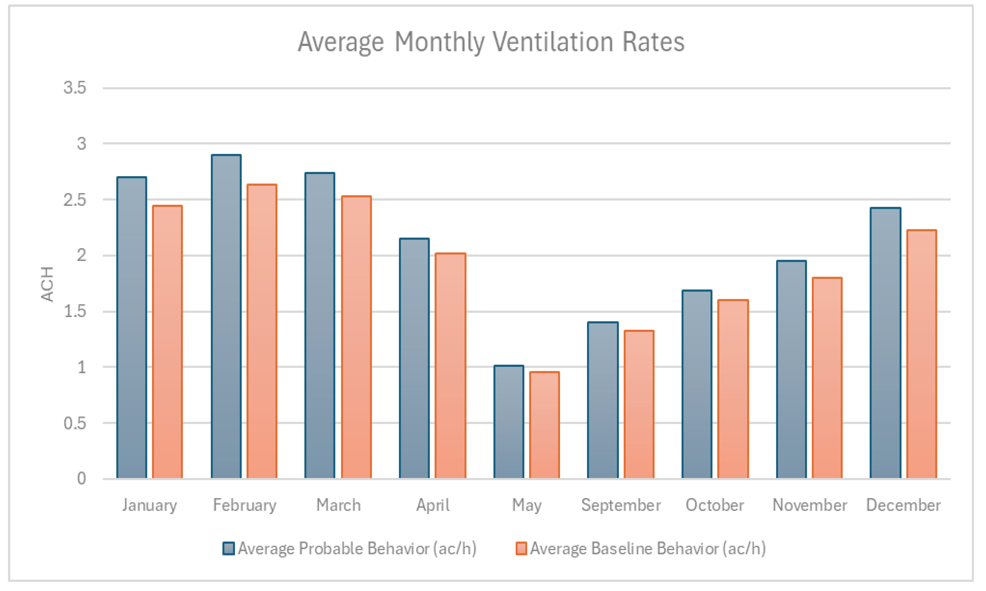
Figure 5.
Natural Ventilation Rates Across Configurations - Baseline Behavior (Scenario A)These gains ranged from +0.9% to +4.0%, with the highest improvements seen in cooler months like May, when strategic use of the west-facing window contributed to better airflow. These findings indicate that while the configurations themselves already support robust natural airflow, occupant engagement can further enhance performance, especially during transitional times of day like early evening.
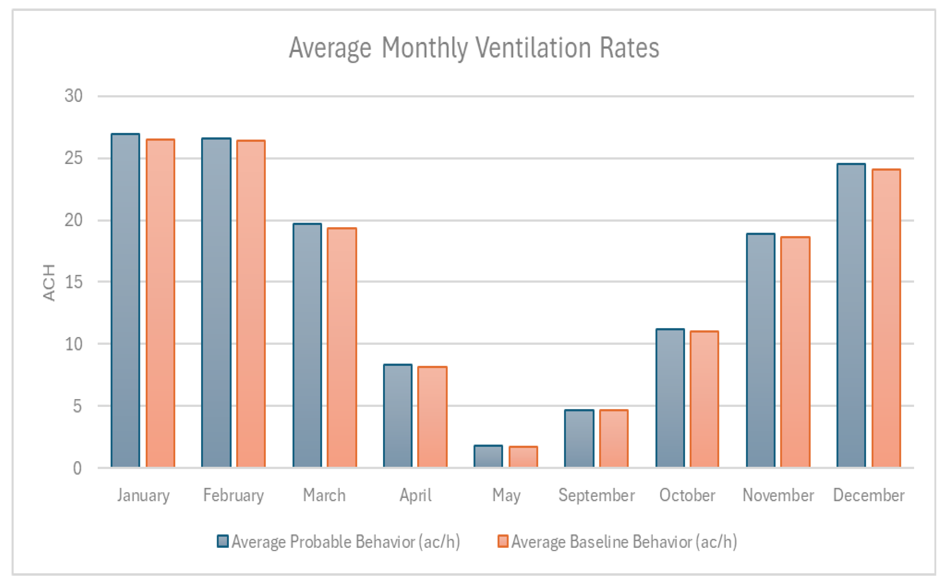
Table 1.
Fixed Input Parameters Used across all Simulations.
| Parameter Type | Fixed Inputs | Description |
|---|---|---|
| Building Dimensions | Typical living room, ceiling height 2.4 m | Living room with wider and smaller wall dimensions, which match standard dimensions for Melbourne homes |
| Wall Construction | Brick veneer, air cavity, reflective sarking, plasterboard | Standard local wall construction |
| Window Specifications | Double-glazed low-E glass, thermally broken aluminium frames | U-value: 2.8–3.2 W/m²·K; SHGC: 0.40–0.50 |
| Weather Data | Hourly temperature, humidity, wind speed, and solar radiation | Melbourne climate, typical meteorological year |
Table 2.
Summary of Window Design Stories and Behavior Model Rationales.
| Design Story | Orientation | Configuration | WWR | Configuration Rational |
|---|---|---|---|---|
| Story 1 | North | Dual window | 45% | -Directly responds to the strongest orientation preferences. -Side-by-side configurations showed high occupant interaction, particularly for achieving fresh air. -Size 45% WWR represents the occupant's desire for ample daylight/view. |
| Story 2 | East-West | Single window | E 40% W 30% |
- Large east-facing window extending towards the ceiling for optimal light, and takes advantage of morning light and passive heating. - The west window helps manage afternoon heat gain. - Providing cross-ventilation. |
| Story 3 | South | Dual window | 30% Each | -Investigate occupant interaction with an orientation known for consistent, diffuse daylight and minimal direct solar heat gain/glare. -Side-by-side configuration, which has high occupant interaction for ventilation and general use. -Moderate 60% WWR, provides substantial natural light, aligning with occupant preference for light/view. |
| Story 4 |
North & South | Dual North Single South |
S 40% N 25% Each |
-Preferred North orientation for potential winter solar gain and ventilation. -The large, ceiling-height south-facing dimension enhances daylight penetration -Design maximizes cross-ventilation potential by utilising both north and south orientations. |
| Story 5 | North &East | Single North Dual South |
N 40% E 25% Each |
Combination of preferred orientations. -The North Window incorporates the strongly preferred North orientation for ventilation and stable daylight. -East Windows: Leverage the benefits of the East morning light |
Table 3.
Behavior Model Rationale by Design Story and Room Scenario.
| Design Story | Orientation | Scenario A | Scenario B | SB Rationale | PB Rationale |
|---|---|---|---|---|---|
| Story 1 | North |  |
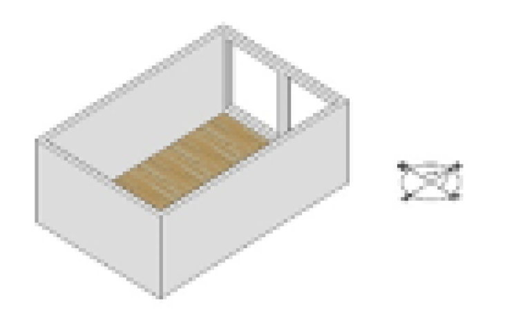 |
Regular morning and evening openings | On wider walls, it increases morning openings for wind; on smaller walls, less frequent due to limited airflow. |
| Story 2 | East and West | 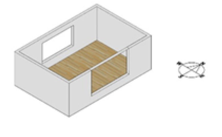 |
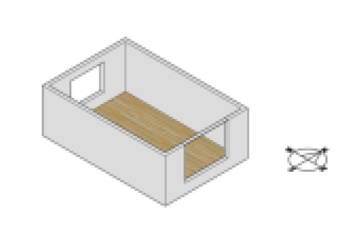 |
Morning openings (east), evening openings (west) | On wider walls, boosts east morning openings for light; on smaller walls, reduces west midday openings for heat control. |
| Story 3 | South | 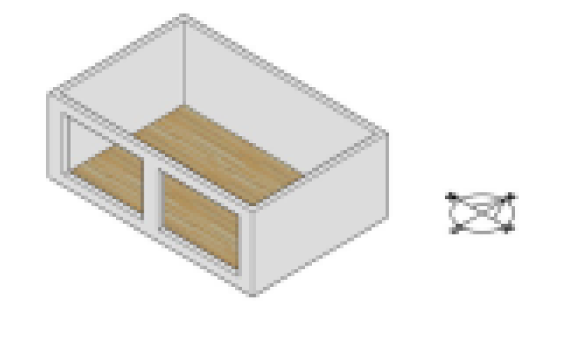 |
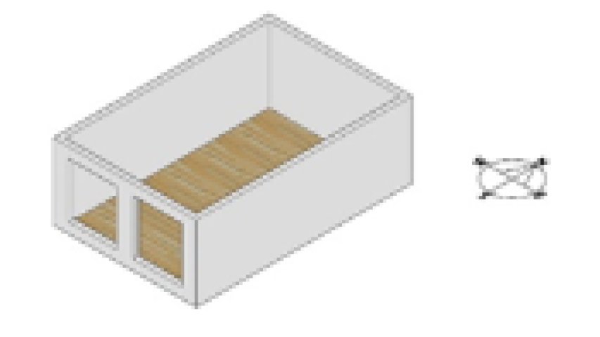 |
Less frequent openings due to limited wind exposure. | On wider walls, reduce midday openings to manage heat; on smaller walls, further limited due to weaker ventilation potential. |
| Story 4 | North and South | 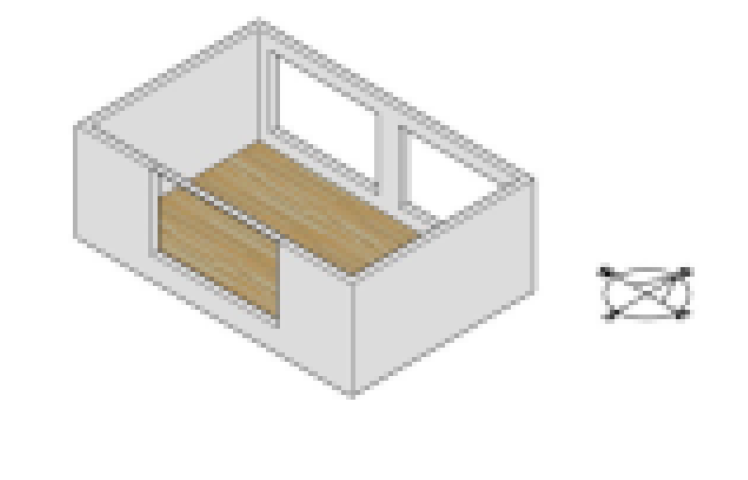 |
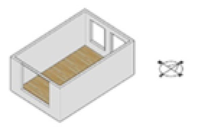 |
Frequent openings for cross-ventilation, especially mornings. | On wider walls, enhances morning cross-ventilation; on smaller walls, reduces south midday openings for heat control. |
| Story 5 | North-East | 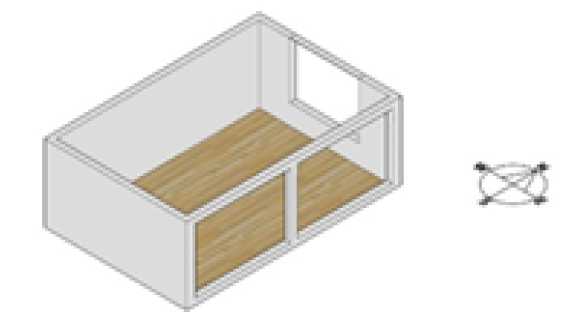 |
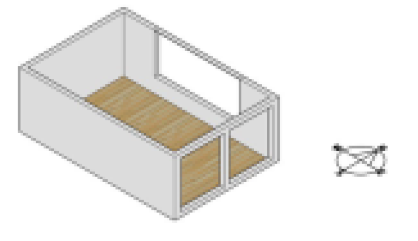 |
East morning openings for light, north for steady ventilation. | On wider walls, boosts east morning openings; on smaller walls, adjusts north for consistent airflow throughout the day. |
Table 4.
Natural Ventilation Performance of North-Facing Windows (Scenario A, SB Model).
| Configuration | Peak (ACH) (Month) | Lowest (ACH) (Month) | Average (ACH) |
|---|---|---|---|
| 1 | 4.67 (March) | 1.95 (May) | 3.47 |
| 2 | 4.52 (March) | 1.89 (May) | 3.36 |
| 3 | 4.40 (March) | 1.89 (May) | 3.31 |
| 4 | 4.31 (March) | 1.86 (May) | 3.23 |
| 5 | 3.95 (March) | 1.72 (May) | 2.97 |
| 6 | 4.06 (March) | 1.78 (May) | 3.06 |
| 7 | 4.06 (March) | 1.77 (May) | 3.06 |
Table 5.
Ventilation and Solar Gain - Design Story 1, Scenario B (Baseline and Probable Behaviors).
| Month | Highest NV Probable (ACH) (Config.) | Lowest NV Probable (ACH) (Config.) | Avg. NV Baseline (ACH) | Avg. NV Probable (ACH) | % Change | Avg. Solar Gain (kWh) | Peak Solar Gain (kWh) (Config.) | Lowest Solar Gain (kWh) (Config.) |
|---|---|---|---|---|---|---|---|---|
| Jan | 4.12 (1) | 3.49 (5) | 3.80 | 4.23 | +11.2% | 228.15 | 238.93 (4) | 219.66 (1) |
| Feb | 4.63 (1) | 3.90 (5) | 4.24 | 4.72 | +11.3% | 235.29 | 275.27 (4) | 219.66 (1) |
| Mar | 4.67 (1) | 3.95 (5) | 4.28 | 4.83 | +12.7% | 294.62 | 408.14 (4) | 219.66 (1) |
| Apr | 3.80 (1) | 3.27 (5) | 3.52 | 3.86 | +9.6% | 291.09 | 404.11 (4) | 219.66 (1) |
| May | 1.95 (1) | 1.72 (5) | 1.84 | 2.05 | +11.3% | 298.98 | 436.76 (4) | 219.66 (1) |
| Sep | 2.41 (1) | 2.16 (5) | 2.29 | 2.51 | +9.5% | 237.18 | 404.32 (4) | 219.66 (1) |
| Oct | 2.92 (1) | 2.55 (5) | 2.74 | 2.97 | +8.7% | 246.09 | 336.10 (4) | 219.66 (1) |
| Nov | 3.00 (1) | 2.60 (5) | 2.78 | 3.08 | +10.8% | 228.13 | 242.85 (4) | 219.66 (1) |
| Dec | 3.67 (1) | 3.13 (5) | 3.37 | 3.70 | +9.6% | 223.04 | 223.81 (4) | 219.52 (2) |
Table 6.
Natural Ventilation Performance of North-Facing Windows (Scenario B, SB Model).
| Configuration | Peak (ACH) (Month) | Lowest (ACH) (Month) | Average (ACH) |
|---|---|---|---|
| 9 | 2.86 (February) | 1.00 (May) | 2.09 |
| 10 | 2.67 (February) | 0.96 (May) | 1.97 |
| 11 | 2.58 (February) | 0.95 (May) | 1.92 |
| 12 | 2.44 (February) | 0.92 (May) | 1.84 |
| 13 | 2.79 (February) | 1.00 (May) | 2.06 |
| 14 | 2.52 (February) | 0.95 (May) | 1.89 |
| 15 | 2.52 (February) | 0.94 (May) | 1.89 |
Table 7.
Ventilation and Solar Gain under SB and PB Models (Scenario B).
| Month | Highest NV Probable (ACH) (Config.) | Lowest NV Probable (ACH) (Config.) | Avg. NV Baseline (ACH) | Avg. NV Probable (ACH) | % Change | Avg. Solar Gain (kWh) | Peak Solar Gain (kWh) (Config.) | Lowest Solar Gain (kWh) (Config.) |
|---|---|---|---|---|---|---|---|---|
| Jan | 2.65 (9) | 2.28 (12) | 2.44 | 2.70 | +10.6% | 148.05 | 149.23 (15) | 146.07 (10) |
| Feb | 2.86 (9) | 2.44 (12) | 2.63 | 2.90 | +10.3% | 171.27 | 171.63 (15) | 168.05 (10) |
| Mar | 2.75 (9) | 2.37 (12) | 2.53 | 2.74 | +8.1% | 251.70 | 254.26 (15) | 248.99 (10) |
| Apr | 2.14 (9) | 1.91 (12) | 2.02 | 2.15 | +6.4% | 249.46 | 251.69 (15) | 246.49 (10) |
| May | 1.00 (9) | 0.92 (12) | 0.96 | 1.01 | +5.1% | 269.41 | 271.97 (15) | 266.36 (10) |
| Sep | 1.41 (9) | 1.29 (12) | 1.33 | 1.40 | +5.2% | 249.51 | 251.86 (15) | 246.65 (10) |
| Oct | 1.70 (9) | 1.51 (12) | 1.60 | 1.69 | +5.5% | 207.85 | 209.49 (15) | 205.12 (10) |
| Nov | 1.92 (9) | 1.70 (12) | 1.80 | 1.95 | +8.6% | 150.15 | 151.62 (15) | 148.42 (10) |
| Dec | 2.40 (9) | 2.10 (12) | 2.23 | 2.43 | +9.0% | 148.62 | 149.94 (15) | 136.96 (10) |
Table 8.
Natural Ventilation Performance of East–West Window Designs (Scenario A).
| Configuration | Peak (ACH) | Lowest (ACH) | Average (ACH) |
|---|---|---|---|
| 1 | 26.83 (January) | 1.81 (May) | 13.83 |
| 2 | 26.82 (January) | 1.79 (May) | 13.79 |
| 3 | 26.74 (January) | 1.79 (May) | 13.77 |
| 4 | 26.58 (January) | 1.73 (May) | 13.54 |
| 5 | 27.22 (January) | 1.80 (May) | 14.02 |
| 6 | 25.40 (January) | 1.65 (May) | 12.70 |
| 7 | 26.44 (January) | 1.74 (May) | 13.45 |
| 8 | 26.31 (January) | 1.74 (May) | 13.38 |
| 9 | 26.46 (January) | 1.77 (May) | 13.43 |
Table 14.
Natural Ventilation Rates Across Stories - Baseline Behavior (Scenario B).
| Configuration | Peak (ACH) (Month) | Lowest (ACH) (Month) | Average (ACH) (Sep–May) |
|---|---|---|---|
| 10 | 15.61 (February) | 0.88 (May) | 8.92 |
| 11 | 15.59 (February) | 0.87 (May) | 8.90 |
| 12 | 16.63 (February) | 0.88 (May) | 8.94 |
| 13 | 15.62 (February) | 0.88 (May) | 8.93 |
| 14 | 15.63 (February) | 0.85 (May) | 8.94 |
| 15 | 15.61 (February) | 0.88 (May) | 8.92 |
| 16 | 15.60 (February) | 0.87 (May) | 8.91 |
| 17 | 16.18 (February) | 0.88 (May) | 8.92 |
| 18 | 15.62 (February) | 0.88 (May) | 8.93 |
Table 15.
Ventilation and Solar Gain - Design Story 3, Scenario B (Baseline and Probable Behaviors).
Table 15.
Ventilation and Solar Gain - Design Story 3, Scenario B (Baseline and Probable Behaviors).
| Month | Highest NV Probable (ACH) (Config.) | Lowest NV Probable (ACH) (Config.) | Avg. NV Baseline (ACH) | Avg. NV Probable (ACH) | % Change | Avg. Solar Gain (kWh) | Peak Solar Gain (kWh) (Config.) | Lowest Solar Gain (kWh) (Config.) |
|---|---|---|---|---|---|---|---|---|
| Jan | 16.47 (12) | 15.95 (17) | 13.82 | 13.47 | -2.5% | 369.65 | 424.69 (3) | 334.32 (5) |
| Feb | 16.63 (12) | 16.18 (17) | 13.91 | 13.74 | -1.2% | 322.39 | 370.33 (3) | 291.50 (5) |
| Mar | 11.89 (12) | 11.49 (17) | 10.17 | 10.11 | -0.6% | 275.41 | 316.28 (3) | 249.11 (5) |
| Apr | 4.76 (12) | 4.59 (17) | 4.09 | 3.92 | -4.2% | 178.04 | 204.54 (3) | 161.06 (5) |
| May | 0.88 (10) | 0.88 (17) | 0.88 | 0.85 | -3.4% | 138.41 | 158.99 (3) | 125.21 (5) |
| Sep | 2.99 (12) | 2.89 (17) | 2.57 | 2.41 | -6.2% | 234.12 | 268.99 (3) | 211.78 (5) |
| Oct | 6.86 (12) | 6.63 (17) | 5.90 | 5.68 | -3.7% | 292.26 | 335.83 (3) | 264.34 (5) |
| Nov | 9.98 (12) | 9.65 (17) | 8.56 | 8.25 | -3.6% | 342.86 | 393.87 (3) | 309.99 (5) |
| Dec | 14.25 (12) | 13.76 (17) | 12.20 | 11.75 | -3.7% | 378.88 | 435.32 (3) | 342.72 (5) |
Table 16.
Natural Ventilation Rates Across Stories - Baseline Behavior (Scenario A).
| Configurations | Peak (ACH) (Month) | Lowest (ACH) (Month) | Average (ACH) |
|---|---|---|---|
| A1 | 36.24 (February) | 3.38 (May) | 21.48 |
| A2 | 35.95 (February) | 3.33 (May) | 21.21 |
| A3 | 36.18 (February) | 3.35 (May) | 21.56 |
| A4 | 36.05 (February) | 3.33 (May) | 21.33 |
| A5 | 35.82 (February) | 3.30 (May) | 21.01 |
| A6 | 35.92 (February) | 3.33 (May) | 21.14 |
| A7 | 35.93 (February) | 3.36 (May) | 21.14 |
| A8 | 36.10 (February) | 3.35 (May) | 21.36 |
| A9 | 35.76 (February) | 3.34 (May) | 21.07 |
| A10 | 35.75 (February) | 3.32 (May) | 20.93 |
Table 17.
Ventilation and Solar Gain - Design Story 4, Scenario A (Baseline and Probable Behaviors).
Table 17.
Ventilation and Solar Gain - Design Story 4, Scenario A (Baseline and Probable Behaviors).
| Month | Highest NV Probable (ACH) (Config.) | Lowest NV Probable (ACH) (Config.) | Avg. NV Baseline (ACH) | Avg. NV Probable (ACH) | % Change | Avg. Solar Gain (kWh) | Peak Solar Gain (kWh) (Config.) | Lowest Solar Gain (kWh) (Config.) |
|---|---|---|---|---|---|---|---|---|
| Jan | 35.90 (1) | 35.75 (10) | 34.04 | 37.00 | +8.7% | 423.94 | 427.89 (3) | 420.58 (10) |
| Feb | 36.24 (1) | 35.75 (10) | 35.97 | 39.41 | +9.6% | 421.31 | 426.44 (3) | 418.49 (10) |
| Mar | 25.60 (1) | 25.40 (10) | 27.31 | 31.00 | +13.5% | 547.37 | 553.22 (3) | 541.82 (10) |
| Apr | 10.25 (1) | 10.15 (10) | 15.09 | 17.71 | +17.4% | 515.99 | 521.83 (3) | 510.71 (10) |
| May | 3.38 (1) | 3.32 (10) | 3.34 | 4.06 | +21.6% | 534.33 | 541.11 (3) | 529.02 (10) |
| Sep | 8.55 (1) | 8.45 (10) | 7.29 | 8.64 | +18.5% | 532.32 | 538.21 (3) | 526.98 (10) |
| Oct | 15.35 (1) | 15.25 (10) | 15.63 | 18.28 | +16.9% | 487.98 | 493.01 (3) | 483.56 (10) |
| Nov | 22.50 (1) | 22.30 (10) | 19.39 | 21.38 | +10.3% | 419.25 | 423.27 (3) | 415.71 (10) |
| Dec | 30.20 (1) | 30.00 (10) | 28.22 | 31.37 | +7.6% | 431.23 | 434.96 (3) | 428.02 (10) |
Table 18.
Natural Ventilation Rates Across Stories - Baseline Behavior (Scenario B).
| Configuration | Peak (ACH) (Month) | Lowest (ACH) (Month) | Average (ACH) (Sep–May) |
|---|---|---|---|
| A1 | 21.41 (January) | 1.87 (May) | 11.22 |
| A2 | 22.58 (February) | 1.63 (May) | 11.45 |
| A3 | 22.30 (February) | 1.64 (May) | 11.05 |
| A4 | 22.44 (February) | 1.72 (May) | 11.33 |
| A5 | 20.87 (February) | 1.60 (May) | 10.47 |
| A6 | 23.75 (February) | 1.77 (May) | 12.09 |
| A7 | 22.12 (February) | 1.64 (May) | 10.88 |
| A8 | 22.57 (February) | 1.75 (May) | 11.28 |
| A9 | 22.26 (February) | 1.66 (May) | 11.11 |
Table 21.
Ventilation and Solar Gain - Design Story 5, Scenario A (Baseline and Probable Behaviors).
Table 21.
Ventilation and Solar Gain - Design Story 5, Scenario A (Baseline and Probable Behaviors).
| Month | Highest NV Probable (ACH) (Config.) | Lowest NV Probable (ACH) (Config.) | Avg. NV Baseline (ACH) | Avg. NV Probable (ACH) | % Change | Avg. Solar Gain (kWh) | Peak Solar Gain (kWh) (Config.) | Lowest Solar Gain (kWh) (Config.) |
|---|---|---|---|---|---|---|---|---|
| Jan | 22.72 (2) | 21.29 (5) | 22.00 | 23.57 | +7.1% | 485.17 | 502.49 (2) | 472.70 (5) |
| Feb | 21.77 (2) | 20.38 (5) | 20.88 | 22.05 | +5.6% | 491.50 | 510.64 (2) | 479.15 (5) |
| Mar | 25.39 (2) | 23.66 (5) | 24.36 | 26.18 | +7.5% | 578.86 | 605.23 (2) | 564.66 (5) |
| Apr | 15.63 (2) | 14.42 (5) | 14.90 | 16.28 | +9.3% | 506.61 | 531.74 (2) | 494.55 (5) |
| May | 5.89 (2) | 5.30 (5) | 5.55 | 5.86 | +5.6% | 501.00 | 527.52 (2) | 488.48 (5) |
| Sep | 10.63 (2,10) | 9.93 (5) | 10.23 | 10.79 | +5.5% | 548.05 | 575.75 (2) | 536.79 (5) |
| Oct | 17.83 (2,8) | 16.58 (5) | 17.24 | 18.89 | +9.6% | 543.71 | 566.28 (2) | 530.11 (5) |
| Nov | 19.19 (2) | 18.04 (7) | 18.50 | 20.05 | +8.4% | 492.50 | 510.21 (2) | 479.97 (5) |
| Dec | 23.01 (2) | 21.00 (5) | 22.16 | 24.61 | +11.1% | 493.05 | 509.82 (2) | 480.14 (5) |
Table 22.
Natural Ventilation Rates Across Stories - Baseline Behavior (Scenario B).
| Configuration | Peak (ACH) (Month) | Lowest (ACH) (Month) | Average (ACH) |
|---|---|---|---|
| 1 | 20.62 (January) | 4.18 (May) | 15.47 |
| 2 | 20.92 (January) | 4.23 (May) | 15.56 |
| 3 | 21.87 (March) | 4.20 (May) | 15.99 |
| 4 | 21.73 (March) | 4.14 (May) | 15.85 |
| 5 | 22.94 (December) | 4.12 (May) | 15.93 |
| 6 | 20.87 (January) | 4.21 (May) | 15.48 |
| 7 | 21.43 (March) | 4.11 (May) | 15.32 |
| 8 | 20.98 (January) | 4.19 (May) | 15.54 |
| 9 | 20.47 (January) | 4.13 (May) | 15.41 |
| 10 | 20.80 (January) | 4.19 (May) | 15.50 |
Disclaimer/Publisher’s Note: The statements, opinions and data contained in all publications are solely those of the individual author(s) and contributor(s) and not of MDPI and/or the editor(s). MDPI and/or the editor(s) disclaim responsibility for any injury to people or property resulting from any ideas, methods, instructions or products referred to in the content. |
© 2025 by the authors. Licensee MDPI, Basel, Switzerland. This article is an open access article distributed under the terms and conditions of the Creative Commons Attribution (CC BY) license (http://creativecommons.org/licenses/by/4.0/).
Copyright: This open access article is published under a Creative Commons CC BY 4.0 license, which permit the free download, distribution, and reuse, provided that the author and preprint are cited in any reuse.


