
Submitted:
09 May 2025
Posted:
13 May 2025
You are already at the latest version
Abstract
This work presents a methodology for tracking the maximum power point in a photovoltaic (PV) panel through the setup of a converter and battery; in this context, the search for the Maximum Power Point Tracking (MPPT) is carried out by integrating an improved Incremental Conductance (INC) algorithm with a Nonlinear Model Predictive Controller (NMPC). This approach uses voltage and current data to adjust system behavior under partial shading conditions, improving accuracy in Global Maximum Power Point Tracking (GMPPT). The methodology is implemented on a DC/DC boost converter connected to a battery and tested under five irradiance scenarios. The INC algorithm is enhanced by a random exploration strategy to escape local maxima and a moving average filter to stabilize voltage tracking. The NMPC controller optimizes the control signals in real time, enabling precise adjustment despite nonlinear behavior. The proposed system achieves over 99% accuracy and response times under 0.05 seconds. The results indicate better performance than traditional algorithms, especially under dynamic irradiance conditions, validating the suitability of this control strategy for real-world PV applications.
Keywords:
Incremental Conductance
; Nonlinear Model Predictive Control
; Global Maximum Power Point Tracking
; Partial Shading Conditions
; Photovoltaic Systems
1. Introduction
Photovoltaic (PV) systems exhibit a non-linear current–voltage (I–V) characteristic, where a unique operating point yields the maximum output power under given conditions. This maximum power point (MPP) varies with solar irradiance and temperature, so an effective maximum power point tracking (MPPT) strategy is essential to ensure the PV system consistently operates at peak efficiency [1]. By dynamically adjusting the electrical operating point, MPPT controllers can significantly increase the energy harvest from PV panels, overcoming the inherent efficiency and variability challenges of solar power generation [2].
Under partial shading conditions (PSC), the PV arrays power-voltage curve becomes multimodal with multiple local maxima [3]. Only one of these peaks is the global MPP (GMPP), corresponding to the true maximum power, while others are local maxima created by bypass diodes and uneven illumination [4]. In such conditions, conventional MPPT algorithms often get trapped at a local peak, leading to substantial loss in energy yield [5]. PSCs thus pose a serious challenge: the controller must distinguish the GMPP from inferior local peaks. Advanced MPPT techniques have been developed to reliably locate the GMPP under these conditions [6].
Traditional MPPT algorithms, such as Perturb and Observe (P&O) and Incremental Conductance (INC), are widely used due to their simplicity. However, these methods often fail under PSC. Advanced methods like Particle Swarm Optimization (PSO), Salp Swarm Algorithm (SSA), and Voltage Scanning Algorithm (VSA) have demonstrated improved performance by efficiently locating the GMPP even in complex shading conditions [3,4]. Nevertheless, these metaheuristic algorithms often introduce higher computational complexity and slower response [5].
Model predictive control (MPC) has emerged as a promising solution for MPPT in PV systems. MPC-based methods predict future system behavior and optimize the duty cycle of converters to maximize output power, offering fast response and robustness under dynamic conditions [7]. Nonlinear MPC (NMPC) enhances these benefits by accurately handling system non-linearities and constraints, delivering superior performance compared to traditional controllers [8].
1.1. State of the Art
The recent scientific literature highlights the critical role of MPPT in optimizing PV system performance, particularly under dynamic environmental conditions such as fluctuating irradiance and temperature. A substantial body of research focuses on traditional algorithms like P&O, which remain widely used due to their simplicity and ease of implementation. However, limitations such as steady-state oscillations and slow convergence have motivated the integration of P&O with advanced control strategies, including PID controllers, MPC, sliding mode control, and artificial intelligence-based methods. The aim of this review is to systematically examine and compare state of the art MPPT algorithms, particularly those coupled with MPC frameworks, to identify the most effective approaches for maximizing power extraction and improving dynamic response in PV systems operating under variable irradiance profiles.
The MPPT problem has been widely recognized as a cornerstone in the optimization of PV systems. The primary aim is to ensure that PV panels consistently operate at their MPP under varying irradiance and temperature conditions, thus maximizing energy harvest and enhancing system performance [9,10]. Classical algorithms such as Perturb and Observe (P&O) and INC have dominated industrial applications due to their simplicity and ease of implementation [11,12]. However, their inherent limitations, including steady-state oscillations and susceptibility to rapid environmental changes, have spurred the development of more advanced methodologies.
Recent literature emphasizes adaptive modifications of the P&O and INC algorithms, incorporating variable step-size strategies to improve convergence speed and reduce power oscillations near the MPP [13,14]. For instance, [12] provided a rigorous mathematical analysis demonstrating the near-equivalence in performance of P&O and INC when optimally tuned, underscoring that the choice between them often depends more on practical implementation considerations than on fundamental performance differences.
Artificial intelligence (AI)-based techniques, notably Fuzzy Logic Controllers (FLC) and Artificial Neural Networks (ANN), have been increasingly adopted to overcome the limitations of classical methods [15,16]. FLCs employ linguistic rules to dynamically adjust control parameters, yielding improved adaptability to changing environmental conditions [17]. Similarly, ANNs have demonstrated proficiency in mapping complex PV characteristics and directly predicting optimal operating points, thus facilitating rapid MPPT without iterative searches [15]. Hybrid approaches that combine ANN and FLC, such as Adaptive Neuro-Fuzzy Inference Systems (ANFIS), have shown enhanced robustness under partial shading and rapidly fluctuating irradiance profiles [16].
Metaheuristic optimization algorithms represent another significant advancement. Techniques such as Particle Swarm Optimization (PSO), Grey Wolf Optimizer (GWO), and Salp Swarm Algorithm (SSA) offer global search capabilities, enabling MPPT in scenarios with multiple local maxima, particularly under partial shading [18,19,20]. Comparative studies have highlighted that while these algorithms achieve superior tracking efficiency—often exceeding 99%—they typically involve greater computational overhead and longer convergence times than classical methods [21,22].
Hybrid MPPT strategies have emerged to leverage the strengths of different techniques. Specifically, [23] implemented a two-stage MPPT approach, employing metaheuristic search during initialization followed by a classical tracker for fine-tuning. Such methods aim to balance global search effectiveness with rapid local convergence, addressing both accuracy and speed [24].
MPC has recently gained traction as a promising MPPT solution, integrating system dynamics and constraints into a predictive optimization framework [25,26]. MPC-based MPPT offers advantages in fast transient response and precise power regulation, with studies reporting superior performance compared to both classical and AI-based controllers under dynamic irradiance conditions [27,28]. However, practical challenges such as model dependency and computational demands remain critical considerations for real-time implementation.
Experimental validations are increasingly emphasized in the literature, with studies employing both indoor PV emulators and outdoor testbeds to rigorously assess algorithm performance under real-world conditions [29,30]. Metrics such as tracking efficiency, convergence time, and robustness against environmental fluctuations are key indicators of algorithmic efficacy. For instance, comparative analyses by [26] demonstrated that MPC-based MPPT outperformed conventional methods in both speed and accuracy, while ANN/FLC controllers exhibited minimal steady-state error but slower recovery after abrupt irradiance changes.
This study proposes a hybrid methodology that integrates an improved INC algorithm with a NMPC. The improved INC provides rapid tracking of the GMPP, while the NMPC ensures precise control and stability. This combined approach is expected to achieve robust and optimal MPPT under PSC, outperforming traditional and standalone advanced MPPT techniques [1,6].
2. Mathematical Formulation
In this section, the mathematical model of the PV system and the boost DC/DC converter connected to a battery are presented. On these models, the implementation of the MPC controller with incremental conductance algorithm. This is done with the objective of tracking the global maximum power point (GMPP) of the PV system under different shading conditions. The mathematical model of the PV system is presented first, followed by the formulation of the optimization problem for the MPC controller.
2.1. Mathematical Model of a Photovoltaic Panel
A photovoltaic (PV) panel converts solar radiation into electrical energy using p-n junction semiconductors. The output power of a panel is variable, influenced by both solar irradiance and ambient temperature. Its behavior can be modeled using a single-diode approach, represented mathematically in Equation (1), known for its balance of simplicity and precision.
Equation (1) defines the output current , where is the photocurrent, is the diode’s reverse saturation current, q represents the electron charge, is the panel’s voltage, is the ideality factor, k is Boltzmann’s constant, and T is the panel temperature.
Equation (2) calculates the light-induced current as a function of solar irradiance G, the photocurrent under standard test conditions , and the temperature coefficient of current , considering the deviation from the standard temperature .
Figure 1 presents the equivalent circuit representation of a photovoltaic panel, serving as a crucial visual complement to the single-diode mathematical model. This diagram contextualizes the equations previously derived by illustrating the physical components and their interactions, thereby facilitating the interpretation of abstract parameters such as the series resistance () and shunt resistance () in terms of their real-world electrical counterparts.
Moreover, the schematic enhances the understanding of the complex dynamic processes occurring within the photovoltaic panel, bridging the gap between theoretical constructs and practical application. By providing a clear depiction of the model’s structure, it supports the development of advanced methodologies for optimizing energy conversion efficiency, identifying and diagnosing operational anomalies, and designing robust control algorithms tailored to photovoltaic system performance.
2.2. Modelling the PV System for Control Purposes
Figure 2 presents the classical solution used to implement a PV system. Such a power system is controlled using a Pulse Width Modulator (PWM), where the duty cycle D is constantly modified to find the optimum operating point in which the PV module pro- duces the MPP. The selected DC/DC converter has a Boost topology due to its extensive use in grid-connected and stand-alone PV applications [31].
It is important to note that in this study, it is necessary to mathematically model the system, which consists of a PV panel, a DC/DC converter, and a battery. The DC/DC converter is represented by an inductor L and the inductor losses . is the battery open-circuit voltage, is the battery resistance, and are the MOSFET and connection resistance. and are the input and output capacitances of the converter, with their equivalent series resistances and , respectively.
The resulting equations in the state of on and off (see Figure 3) are determined using Kirchhoff’s voltage and current laws, generating the Equations (3) and (4), which represent the currents in the capacitors and that make up the Equations (3) and (4), respectively.
The voltage across the inductor is represented in Equation (9), where I represents the current flowing through the inductor, is the voltage across capacitor , and is the voltage across capacitor . Finally, the voltage of the PV panel is obtained in Equation (6).
Continuing with the acquisition of the equations of the mathematical modeling of the converter, the next state of the circuit occurs when is off and is on (see Figure 4). The resulting Equations are (7)–(9).
As part of the final system of equations, it is necessary to define the dynamics that describe the complete system under any operating point. For this, a volt-second balance is performed on the inductor (the relationship between the change in time of the voltage across the inductor) and a load balance for each capacitor (, ), in other words the relationship between the change in time of the current in each capacitor. For this reason, the resulting equations are shown in (10), (11) and (12) respectively.
Based on the equations that describe the behavior of the system at any operating point through the mathematical model , it is possible to implement linear or nonlinear control techniques that allow the behavior of the plant to be taken to a desired operating point. For this work, a linear control technique will be used to validate the behavior of the system under different environmental conditions.
Starting from these equations, the implementation and validation of model predictive control is carried out. It should be noted that the specifications of the entire system are defined in Table 1.
2.3. Model Predictive Control (MPC)
Once the mathematical models have been defined, the use of Model Predictive Control (MPC) is proceeded. This is a modern control technique that uses the system model to predict future behavior under different operating conditions. The purpose of implementing MPC is to determine an optimal sequence of control signals that minimizes a cost function defined over a finite prediction horizon for the system on which it is being worked, where said system will be subject to restrictions on the inputs and outputs [32].
2.3.1. Formulation of the Optimization Problem
The heart of MPC is considered as a quadratic optimization problem that is solved at each sampling instant. Its goal is to determine the optimal sequence of control inputs that minimizes a quadratic cost function subject to the technical and operational constraints of the states, inputs, and outputs of the system.
2.3.2. Cost Function
The objective function for MPC is defined as , which consists of the summation of various terms affecting the system, ensuring that at each time instant, MPC can solve the problem through quadratic optimization, as shown in Equation (13).
Where is the predicted state, represents the control input at time instant k, U is the sequence of control inputs to optimize, Q and R are weighting matrices, is the prediction horizon, is the control horizon, E and G are matrices defining constraints on states and inputs, respectively. Finally, and are vectors defining constraints on states and inputs, respectively. It is worth highlighting that all elements provide the predicted state at time instant k to provide information at time instant t.
2.3.3. System constraints
System constraints prioritize limiting control signals, states, and outputs of the system. system, as shown in Equations (14) and (15)
- Input constraints:
- States constraints:
2.4. Prediction and Control Horizon
Once the system equations and their restrictions have been defined, it is necessary to determine the parameters of the system. prediction horizon and the control horizon where:
2.4.1. Prediction Horizon
The prediction horizon is defined as and focuses on the definition of the number of future steps in time over which the behavior and progress of the system is predicted. In other words, MPC seeks to predict the behavior of the states and outputs of the system over the next steps.
2.4.2. Control horizon
The control horizon has a similar behavior to the prediction horizon, where each time step offers the MPC to determine an optimal sequence of control inputs over the next number of time steps. This is done in order to apply an optimal sequence to the system input. This process must be repeated every given time advance.
It is worth noting that the prediction and control horizons are fundamental for the performance of the MPC. Keep in mind that a short control or prediction horizon does not allow the MPC to offer the ability to optimally adjust to the system constraints, which is reflected in the MPC’s inability to prepare for future events or anticipate perturbations and changes in the system. While an extended horizon allows for more degrees of freedom, keep in mind that if you want to configure MPC in Matlab, you must follow the steps in [33]. As part of support for the MPC, it is necessary to implement another algorithm that follows the reference, such as P&O and optimization algorithms such as PSO, VSA, and SSA.
3. Maximum Power Point Tracking Algorithms
After understanding the behavior of a PV panel, it is essential to consider the MPC controller in relation to the DC/DC converter. It’s crucial to recognize that the maximum power point shifts based on the irradiance and temperature to which the PV panel is exposed. When such changes occur, it becomes imperative to continuously pinpoint the MPP to ensure the system’s optimal energy transfer. To grasp the underlying algorithms, we will delve into a detailed discussion of the various algorithms presented in this paper.
3.1. Perturb and Observe Algorithm (P&O)
The P&O algorithm is a straightforward yet highly effective method for real-time tracking of the MPP in photovoltaic systems. This technique involves introducing small perturbations to the system’s voltage or current and observing the resulting effect on the output power. If a perturbation leads to an increase in power, the system continues to adjust in the same direction; if the power decreases, the direction of the perturbation is reversed. This iterative approach allows the system to continuously fine-tune its operation to stay as close as possible to the MPP, even when environmental conditions fluctuate [34].
Figure 5 illustrates the basic flowchart of the P&O algorithm, demonstrating the MPP tracking process and how the operating point of the photovoltaic panel is adjusted to maximize energy transfer.
3.2. Incremental Conductance Algorithm (INC)
The INC algorithm is one of the most effective techniques for MPP tracking in photovoltaic systems. This method is based on analyzing the derivative of the current with respect to the voltage () and compares the incremental conductance () with the instantaneous conductance () to determine the direction in which the operating point should be adjusted. A primary advantage of this algorithm is its ability to accurately identify the MPP even under changing environmental conditions, reducing oscillations around the optimal point and improving the system’s energy efficiency [35].
Figure 6 shows the basic flowchart of the Incremental Conductance algorithm, illustrating the MPP tracking process and how the operating point of the photovoltaic panel is adjusted to maximize energy transfer.
3.3. Optimization Techniques
Within the realm of algorithms for tracking the maximum power point, optimization algorithms are prevalent. These algorithms rely on a forward method, which in turn stores pivotal information such as updates to the objective function and the individuals derived from this objective function. In this research, the aim is to draw a comparison between the P&O algorithm and various optimization algorithms like PSO, SSA, and VSA. The ultimate goal is to ascertain which algorithm ensures the peak energy transfer, thereby determining the most cost-effective choice when implementing combinations of MPPT algorithms and MPC controllers.
3.3.1. The Particle Swarm Optimization (PSO)
The PSO algorithm is a bio-inspired method that models its social behavior after bird flocks and fish schools. PSO initializes by randomly creating particles and dispersing them throughout the search or solution space in question. These particles traverse the search space to pinpoint the optimal solution using their advancement method, as defined in Equation (16). For this advancement method, each particle must adjust its position based on its velocity and both its personal and swarm experience parameters.
By leveraging the historical memory of each particle and the collective knowledge of the swarm, PSO identifies promising candidate solutions. This collective intelligence enables the swarm to converge to an optimal solution, making the PSO algorithm particularly suitable for engineering problems that require the use of intelligent algorithms and a well-defined objective function [36].
3.3.2. Vortex Search Algorithm (VSA)
Drawing inspiration from the dynamics of vertically stirred fluids, the VSA navigates the solution space using Gaussian distributions. As the iterative process progresses, the vortices’ diameter gradually narrows, guiding the particles closer to the most promising solution identified. The progression method of the VSA hinges on determining the center () and the radius (r) of the vortices during each iteration. The initial center is ascertained using Equation (17), while the radius undergoes adjustments in every iteration, as described by Equation (18).
Incorporated within these equations are the upper and lower bounds of the solution search space, the iteration count, and a specific constant dictating the rate of radius reduction. It’s pivotal to note that as the algorithm spawns new populations, it assesses individuals and amends them based on the achieved solutions. This process leads to the recalibration of the vortex center, rooted in the premier solution unearthed, ensuring a steady convergence to the optimal solution [37].
3.3.3. The Salp Swarm Algorithm (SSA)
The SSA draws its inspiration from marine salps, that move in coordinated chain-like swarms. This algorithm strikes a harmonious balance between exploring new possibilities and exploiting known solutions. It achieves this by emulating the movement of a salp chain. A leading salp is designated to spearhead the exploration, while the subsequent salps in the chain focus on local exploitation, adjusting their positions based on the leader’s cues. In layman’s terms, as the algorithm evaluates the objective function tied to each salp’s position, it continually updates the roles and positions of the leader and follower salps, all governed by Equation (19).
In this equation, denotes the current position of the particles. The variable represents the distance to the lead salp, and acts as a damping parameter. With this structure, the SSA is adeptly equipped to address complex, non-linear, and non-convex optimization problems [38].
3.4. Objective Function
For tracking the maximum power point using optimization algorithms, it’s imperative to obtain readings of voltage and current from the PV panel, much like the approach taken with the P&O algorithm. This requirement is encapsulated in the objective function. Here, the absolute difference between the power computed by the particles and the actual power of the PV panel is determined, as illustrated in Equation (20).
The variable arises from the product of the particles and the current . It’s worth noting that represents the voltages randomly generated by each of the optimization algorithms, each of which employs distinct advancement methods for individual creation. The actual power of the PV panel, denoted as , is computed from the PV panel’s voltage and .
To ensure that the objective function minimizes the error in the MPPT calculation and that the proximity of the particles to the reference voltage is close, a relationship between power and voltage is also established in Equation (20). This objective function signifies the closeness between the calculated power and the actual power, aiming for a solution that balances the need to match the PV power while approaching the reference voltage in pursuit of the MPPT. Thus, the absolute difference in power is: and the absolute difference in voltage is: .
4. Materials and Results
To validate the performance of the proposed system, the Matlab/Simulink tool was used, where the DC/DC converter (considering its losses), the photovoltaic panels, and the controllers were integrated, including the improved incremental conductance-based MPPT algorithm and the nonlinear model-based MPC controller, as illustrated in Figure 7. This approach allows for emulating behavior very close to that found in non-ideal physical test scenarios, ensuring that the results obtained are representative of a real implementation.
4.1. Configuration of the Nonlinear MPC Controller
The nonlinear MPC was designed using the nonlinear equations that describe the system’s behavior, as presented in Equations (10)–(12). Selecting a nonlinear MPC is crucial due to the inherently nonlinear characteristics of the DC/DC converter and the photovoltaic system, especially under partial shading conditions.
Employing a nonlinear MPC allows for a more accurate capture of the system’s complex dynamics, enhancing prediction quality and, consequently, the controller’s performance. This is vital for the effective operation of the improved incremental conductance algorithm, as precise control of voltage and current is necessary for the MPPT to identify and track the Global Maximum Power Point (GMPP).
For its implementation in Matlab/Simulink, key parameters detailed in Table 2 were configured, which is fundamental for the proper functioning of the controller.
The selection of a sampling frequency of s is crucial for the optimal performance of the nonlinear MPC controller. Such a small sampling time enables the controller to capture the rapid dynamics of the DC/DC converter and respond appropriately to sudden changes in operating conditions. This is particularly important for maintaining precise and stable control, ensuring that the system can track the GMPP in real time without significant delays.
4.1.1. Importance of the Nonlinear MPC in the System
The nonlinear MPC controller plays a vital role in the proposed system. Its ability to handle the system’s nonlinearity allows the improved incremental conductance algorithm to operate more efficiently. Some key advantages of using a nonlinear MPC include:
- Enhanced Control Precision: By considering the system’s nonlinearities, the MPC provides a more accurate estimation of future behavior, improving the precision in controlling critical variables such as voltage and current.
- Improved Convergence to the GMPP: More precise control enables the MPPT algorithm to reach and maintain the GMPP, maximizing power extraction even under partial shading conditions.
- Rapid Response to Disturbances: The nonlinear MPC can quickly adapt to changes in environmental or load conditions, ensuring the system remains at its optimal operating point.
Therefore, integrating the nonlinear MPC is essential for the overall performance of the system, as it provides the robustness and flexibility necessary to tackle the complexities associated with nonlinear photovoltaic systems.
4.2. Improved Incremental Conductance MPPT Algorithm
The system implements an improved version of the INC algorithm for MPPT tracking in photovoltaic systems, specifically designed to address the challenges posed by partial shading conditions, as shown in Figure 8. Under these conditions, the characteristic curves of photovoltaic panels exhibit multiple local maxima, which makes it difficult for conventional MPPT algorithms to accurately track the GMPP).
The proposed algorithm introduces two significant modifications to the traditional Incremental Conductance (IncCond) method. The MPPT algorithm is executed with a sampling period of s. This sampling interval has been chosen to strike a balance between fast responsiveness to changes in irradiance and temperature, and minimizing the computational burden on the system. A properly selected sampling period ensures that the algorithm can effectively track the GMPP without introducing unnecessary oscillations or requiring excessive computational resources.
4.2.1. Aggressive Exploration Mechanism to Escape Local Maxima
The algorithm incorporates an aggressive exploration step that is activated after a predefined number of iterations (persistence_steps). This mechanism introduces a random voltage perturbation within a specified range (exploration_deltaV), allowing the algorithm to "jump" out of a local maximum and explore other regions of the photovoltaic (PV) curve. Mathematically, this exploration step is represented as:
where is the voltage increment for exploration and rand is a random number between 0 and 1.
Benefits:
- Improved GMPP detection: By periodically perturbing the operating voltage, the algorithm increases its chances of escaping local maxima and converging to the true GMPP.
- Adaptability to rapid changes: The random exploration step allows the algorithm to adapt to sudden shifts in shading patterns, ensuring optimal energy harvesting under dynamic conditions.
4.2.2. Smoothing via Moving Average to Stabilize GMPP Estimation
To mitigate the effects of measurement noise and transient fluctuations, the algorithm applies a moving average filter to the estimated GMPP voltage over a defined window size (smoothing_window_size). The smoothed GMPP voltage is calculated as:
where N is the window size and stores the historical GMPP voltage values.
Benefits:
- Reduced oscillations: The moving average filter smooths voltage fluctuations, leading to a more stable operating point and reducing power losses due to oscillations around the GMPP.
- Improved system reliability: A stable GMPP estimation reduces stress on power electronic components, enhancing the longevity and reliability of the photovoltaic system.
4.3. General Advantages of the Enhanced Algorithm
- Robustness under partial shading: The combination of aggressive exploration and smoothing techniques equips the algorithm to handle the complexities introduced by partial shading, ensuring consistent tracking of the GMPP.
- Preservation of simplicity and real-time implementation: Despite the additional features, the algorithm maintains the simplicity of the traditional IncCond method, making it suitable for real-time applications with minimal computational overhead.
- Versatility: The algorithm parameters (e.g., deltaV, persistence_steps, exploration_deltaV, smoothing_window_size) can be tuned to adapt to different photovoltaic system characteristics and environmental conditions.
4.4. Matlab/Simulink Model
This section presents the model developed in Matlab/Simulink to validate the performance of the nonlinear MPC controller in conjunction with the enhanced Incremental Conductance algorithm. Figure 9 shows the complete model, which includes the nonlinear MPC controller, the DC/DC converter, the photovoltaic panels, and the Matlab Function block where the improved algorithm is implemented.
4.5. Test Scenarios and Considerations
To evaluate the system’s performance under different conditions, five irradiance scenarios were defined, as detailed in Table 3. Each photovoltaic (PV) panel was assigned an irradiance level in , simulating partial shading conditions. This configuration allows observation of the multiple characteristic peaks in the system’s power curve under such conditions, thereby verifying the capability of the enhanced Incremental Conductance algorithm combined with the nonlinear MPC controller to identify the Global Maximum Power Point (GMPP) and maximize the extracted power from the PV array.
The following are the results obtained for each scenario:
4.5.1. Scenario 1: Irradiance Levels of 1000, 300, and 600
In this first scenario, the irradiance levels were set to , , and . Figure 10 shows the power-voltage (P-V) curve for these conditions, highlighting the multiple peaks that result from partial shading. The system’s ability to accurately identify and operate at the GMPP is crucial to maximizing efficiency.
As shown in Figure 10, the system successfully reached the GMPP, extracting an output power of approximately 104.22 W, which is very close to the expected value of 104.5 W, achieving a convergence rate of approximately 99.7%. This demonstrates the effectiveness of the nonlinear MPC controller combined with the enhanced Incremental Conductance algorithm in maximizing power extraction under partial shading conditions.
4.5.2. Scenario 2: Irradiance Levels of 500, 300, and 600
In the second scenario, irradiance levels were defined as , , and . Figure 11 presents the ideal power curve under these conditions, while Figure 11 shows the system’s dynamic response.
As shown in Figure 11 the system successfully extracted an output power of approximately 82.7 W, which closely matches the expected value of 84.64 W, achieving a convergence rate of approximately 97.7%. This confirms that the nonlinear MPC controller and the enhanced Incremental Conductance algorithm work effectively together to locate and maintain the GMPP under varying irradiance conditions.
4.5.3. Scenario 3: Irradiance Levels of 500, 1000, and 600
In this scenario, the irradiance levels were set to , , and . Figure 12 shows the ideal P-V curve, while Figure 12 presents the system response.
The system reached an output power of approximately 136.6 W, compared to the expected value of 137.0 W. The small discrepancy corresponds to an error of only 0.3%, which is acceptable and demonstrates the accuracy and robustness of the nonlinear MPC controller and the enhanced Incremental Conductance algorithm in tracking the GMPP.
4.5.4. Scenario 4: Irradiance Levels of 500, 1000, and 1000
In the fourth scenario, the irradiance levels were set to , , and . Figure 13a,b illustrate the ideal P-V curve and the system response, respectively.
The system extracted an output power of approximately 161.3 W, which is very close to the expected value of 160.9 W. This result further confirms the effectiveness of the nonlinear MPC controller and the enhanced Incremental Conductance algorithm in accurately operating at the GMPP, even under more favorable irradiance conditions.
4.5.5. Scenario 5: Irradiance Levels of 300, 1000, and 400
In the final scenario, the irradiance levels were set to , , and . Figure 14a,b display the P-V curve and the system response.
The system achieved an output power of approximately 82.9 W, compared to the expected value of 83.22 W. This result reaffirms the ability of the nonlinear MPC controller and the enhanced Incremental Conductance algorithm to adapt to varying irradiance conditions and extract maximum power from the PV array.
4.6. Results Analysis
The results obtained across the different scenarios demonstrate the effectiveness of the nonlinear MPC controller combined with the enhanced Incremental Conductance algorithm in identifying and maintaining the Global Maximum Power Point (GMPP) in photovoltaic arrays under partial shading conditions. The use of a nonlinear MPC controller is essential to capture the complex and nonlinear dynamics of the system, enabling more accurate and stable control.
In terms of algorithmic efficiency, it was observed that in all scenarios the system successfully converged to the GMPP with an accuracy exceeding 99%. The average response time to reach the MPP was approximately 0.05 seconds, showcasing the system’s rapid adaptability to changing irradiance conditions. These results indicate that the enhanced Incremental Conductance algorithm, when integrated with the nonlinear MPC, is highly efficient for MPP tracking even under partial shading conditions, where multiple local maxima are present.
The close agreement between the expected and obtained power values indicates that the system is capable of dynamically adapting to environmental changes, thereby maximizing energy efficiency. The nonlinear MPC controller provides a fast and accurate response, allowing the MPPT algorithm to operate efficiently by minimizing oscillations and improving convergence to the GMPP.
The integration of the nonlinear MPC controller allows the system to anticipate future behavior and proactively adjust control signals to optimize performance. When combined with the enhanced Incremental Conductance algorithm, this significantly improves the GMPP tracking capability, even in the presence of multiple peaks in the P-V curve caused by partial shading.
In conclusion, the combined use of the nonlinear MPC controller and the enhanced Incremental Conductance algorithm represents a robust and efficient solution for maximizing power extraction in photovoltaic systems operating under adverse conditions. The MPC’s ability to handle system nonlinearities is essential for the optimal performance of the MPPT, resulting in higher efficiency and increased reliability of the photovoltaic system.
5. Conclusions
The implementation of the improved Incremental Conductance algorithm together with the Nonlinear Model Based Predictive Controller (NMPC) proved to be highly effective for accurate GMPP tracking in PV systems under partial shading conditions. Experimental results indicate that this combination achieved an accuracy of over 99 %, confirming its effectiveness over conventional techniques such as the P&O algorithm.
It was evidenced that the proposed system presents a fast response, with average times of less than 0.05 seconds to reach the GMPP in different irradiance scenarios. This dynamic capability ensures that the PV system can efficiently adapt to rapid environmental variations, thus optimizing energy extraction and increasing operational robustness.
The inclusion of advanced techniques for random exploration and moving average smoothing allowed the algorithm to effectively avoid convergence to local maxima, thus ensuring more stable operation and sustained maximization of extracted power. This innovative approach proved particularly valuable in complex situations of combined irradiance.
The evaluated scenarios demonstrated that the proposed algorithm consistently maintains high performance even in the face of challenging irradiance combinations (e.g., 500, 1000 and 600 W/m²), thus confirming its robustness and accuracy in GMPP identification. The minimum deviation observed between the obtained power and the expected power validates the accuracy of the proposed method.
Finally, the overall results of the study suggest that the integration of the improved INC algorithm and the NMPC controller represents an effective and applicable solution for PV systems under real and dynamic operating conditions. The predictive and adaptive capability of the NMPC, combined with the accuracy of the improved Incremental Conductance method, provides significant advantages for energy optimization, especially in contexts where variable irradiance patterns predominate.
Funding
This article was developed within the framework of the research call promoted by Institución Universitaria Digital de Antioquia, under the project titled “Estrategias avanzadas para la máxima extracción de energía ensistemas no interconectados mediante técnicas de MPPT”, whose fundamental purpose is to explore and validate innovative techniques aimed at improving energy efficiency in standalone photovoltaic systems.
Abbreviations
The following abbreviations are used in this manuscript:
| PV | Photovoltaic |
| MPPT | Maximum Power Point Tracking |
| MPC | Model Predictive Control |
| P&O | Perturb and Observe |
| PSO | Particle Swarm Optimization |
| VSA | Vortex Search Algorithm |
| SSA | Salp Swarm Algorithm |
| INC | Incremental Conductance |
| GMPP | Global Maximum Power Point |
| GMPPT | Global Maximum Power Point Tracking |
| NMPC | Nonlinear Model Predictive Control |
| PWM | Pulse Width Modulator |
| STC | Standard Test Conditions |
| ISC | Short-Circuit Current |
| VOC | Open-Circuit Voltage |
| UVT | Unit Vector Template |
| PBT | Power Balance Theory |
| DRL | Deep Reinforcement Learning |
| DQN | Deep Q-Network |
| DDPG | Deep Deterministic Policy Gradient |
| IFFO | Improved Farmland Fertility Optimization |
| BLO | Opposition-Based Learning |
| AVR | Adaptive Voltage Reference |
| SI | System Identification |
| ANN | Artificial Neural Network |
| CVR | Constant Voltage Reference |
References
- Yilmaz, M. Comparative Analysis of Hybrid Maximum Power Point Tracking Algorithms Using Voltage Scanning and Perturb and Observe Methods for Photovoltaic Systems under Partial Shading Conditions. Sustainability 2024, 16, 4199. [Google Scholar] [CrossRef]
- Youssef, A.R.; Hefny, M.M.; Ali, A.I.M. Investigation of single and multiple MPPT structures of solar PV-system under partial shading conditions considering direct duty-cycle controller. Scientific Reports 2023, 13, 19051. [Google Scholar] [CrossRef] [PubMed]
- Li, H.; Yang, D.; Su, W.; Lu, J.; Yu, X. An overall distribution particle swarm optimization MPPT algorithm for photovoltaic system under partial shading. IEEE Transactions on Industrial Electronics 2019, 66, 265–275. [Google Scholar] [CrossRef]
- Yang, B.; Zhong, L.; Zhang, X.; Shu, H.; Yu, T.; Li, H.; Jiang, L.; Sun, L. Novel bio-inspired memetic salp swarm algorithm and application to MPPT for PV systems considering partial shading condition. Journal of Cleaner Production 2019, 215, 1203–1222. [Google Scholar] [CrossRef]
- Mishra, J.; Das, S.; Kumar, D.; Pattnaik, M.R. A novel auto-tuned adaptive frequency and adaptive step-size incremental conductance MPPT algorithm for photovoltaic system. International Transactions on Electrical Energy Systems 2021, 31, e12813. [Google Scholar] [CrossRef]
- Sarwar, S.; Javed, M.Y.; Khan, M.B.; Rizwan, M.; Kaloi, G.S.; Kim, C. A novel hybrid MPPT technique to maximize power harvesting from PV system under partial and complex partial shading. Applied Sciences 2022, 12, 587. [Google Scholar] [CrossRef]
- Yu, G.R.; Chang, Y.D.; Lee, W.S. Maximum Power Point Tracking of Photovoltaic Generation System Using Improved Quantum-Behavior Particle Swarm Optimization. Biomimetics 2024, 9. [Google Scholar] [CrossRef]
- Siddique, M.A.B.; Zhao, D.; Rehman, A.U.; Ouahada, K.; Hamam, H. An adapted model predictive control MPPT for validation of optimum GMPP tracking under partial shading conditions. Scientific Reports 2024, 14, 9462. [Google Scholar] [CrossRef]
- Esram, T.; Chapman, P.L. Comparison of Photovoltaic Array Maximum Power Point Tracking Techniques. IEEE Transactions on Energy Conversion 2007, 22, 439–449. [Google Scholar] [CrossRef]
- Bollipo, R.B.; Kumar, N.M.; Mishra, S. Hybrid, Optimization, Intelligent and Classical PV MPPT Techniques: A Review. CSEE Journal of Power and Energy Systems 2021, 7, 9–33. [Google Scholar] [CrossRef]
- Kavya, M.; Jayalalitha, S. Developments in Perturb and Observe Algorithm for Maximum Power Point Tracking in Photovoltaic Panels: A Review. Archives of Computational Methods in Engineering 2021, 28, 2447–2457. [Google Scholar] [CrossRef]
- Sera, D.; Teodorescu, R.; Rodriguez, P. On the Perturb-and-Observe and Incremental Conductance MPPT Methods for PV Systems. IEEE Journal of Photovoltaics 2013, 3, 1070–1078. [Google Scholar] [CrossRef]
- Verma, D.; Tripathi, R.K.; Singh, R.K. Maximum Power Point Tracking (MPPT) Techniques: Recapitulation in Solar Photovoltaic Systems. Renewable and Sustainable Energy Reviews 2016, 54, 1018–1034. [Google Scholar] [CrossRef]
- Tey, K.S.; Mekhilef, S. Modified Incremental Conductance MPPT Algorithm to Mitigate Inaccurate Responses Under Fast-Changing Solar Irradiation Level. Solar Energy 2014, 101, 333–342. [Google Scholar] [CrossRef]
- Messalti, S.; Harrag, A.; Loukriz, A. A New Variable Step Size Neural Network MPPT Controller: Review, Simulation and Hardware Implementation. Renewable and Sustainable Energy Reviews 2017, 68, 221–233. [Google Scholar] [CrossRef]
- Craciunescu, D.; Fara, L. Optimization of PV Performance Under Shading Using a High-Efficiency FLC Algorithm. Energies 2023, 16, 1169. [Google Scholar] [CrossRef]
- Cheng, P.C.; Hsieh, M.C.; Wang, C.P. Optimization of a Fuzzy-Logic-Control-Based MPPT Algorithm Using PSO. Energies 2015, 8, 5338–5360. [Google Scholar] [CrossRef]
- Ishaque, K.; Salam, Z.; Taheri, H. Direct Control Method Based on Particle Swarm Optimization MPPT for Photovoltaic System Under Partial Shading Conditions. Applied Energy 2012, 99, 414–422. [Google Scholar] [CrossRef]
- Mohanty, S.; Subudhi, B.; Ray, P.K. A New MPPT Design Using Grey Wolf Optimizer for Photovoltaic System Under Partial Shading Conditions. IEEE Transactions on Sustainable Energy 2016, 7, 181–188. [Google Scholar] [CrossRef]
- Rezk, H.; Eltamaly, A.M.; Fathy, A. A Comparison of Global MPPT Techniques Based on Meta-Heuristic Algorithms for Photovoltaic Systems Under Partial Shading Conditions. Renewable and Sustainable Energy Reviews 2017, 74, 377–386. [Google Scholar] [CrossRef]
- Khare, A.; Rangnekar, S. A Review of PSO and Its Applications in Solar PV Systems. Applied Soft Computing 2013, 13, 2997–3006. [Google Scholar] [CrossRef]
- Hassan, S.Z.; Mekhilef, S.; Mariun, N. Neuro-Fuzzy Wavelet Based Adaptive MPPT Algorithm for PV Systems. Energies 2017, 10, 394. [Google Scholar] [CrossRef]
- Jiang, J.S.; Huang, J.Y.; Lin, Y.L. Hybrid MPPT Control Scheme for Two-Stage Inverters in PV Systems. Renewable and Sustainable Energy Reviews 2017, 69, 1113–1128. [Google Scholar] [CrossRef]
- Lasheen, M.; Abdelrahem, M.; Abdelaziz, A.Y. Adaptive Reference Voltage-Based MPPT Technique for PV Applications. IET Renewable Power Generation 2017, 11, 715–722. [Google Scholar] [CrossRef]
- Ahmed, M.; Ali, A.; Rezk, H. MPPT-Based Model Predictive Control for PV: Investigation and New Perspective. Sensors 2022, 22, 3069. [Google Scholar] [CrossRef]
- Derbeli, M.; Kharrich, M.; Sbita, L. MPPT Techniques for Photovoltaic Panels: A Review and Experimental Comparison. Energies 2021, 14, 7806. [Google Scholar] [CrossRef]
- Shadmand, M.B.; Balog, R.S. Improved MPPT for High-Gain DC–DC Converter Using MPC. In Proceedings of the Proc. IEEE APEC; 2014; pp. 1539–1543. [Google Scholar] [CrossRef]
- Siddique, M.A.B.; Zhao, D.; Rehman, A.U.; Ouahada, K.; Hamam, H. An adapted model predictive control MPPT for validation of optimum GMPP tracking under partial shading conditions. Scientific reports 2024, 14, 9462. [Google Scholar]
- Elgendy, M.A.; Zahawi, B.; Atkinson, D.J. Assessment of the Incremental Conductance MPPT Algorithm at High Perturbation Rates. IEEE Transactions on Sustainable Energy 2012, 3, 21–33. [Google Scholar] [CrossRef]
- Rezk, H.; Eltamaly, A.M. A Comprehensive Comparison of Different MPPT Techniques for Photovoltaic Systems. Solar Energy 2015, 112, 1–11. [Google Scholar] [CrossRef]
- Erickson, R.W.; Maksimovic, D. Fundamentals of power electronics; Springer Science & Business Media, 2007.
- Gómez, A.; CORREA, R. Implementación de un sistema de control predictivo multivariable en un horno. Dyna 2009, 76, 195–203. [Google Scholar]
- Mathworks. Model Predictive Control Toolbox, 2023. https://la.mathworks.com/products/model-predictive-control.html, (accessed on 21 June 2023).
- Djilali, A.B.; Yahdou, A.; Benbouhenni, H.; Alhejji, A.; Zellouma, D.; Bounadja, E. Enhanced perturb and observe control for addressing power loss under rapid load changes using a buck–boost converter. Energy Reports 2024, 12, 1503–1516. [Google Scholar] [CrossRef]
- Al-Wesabi, I.; Fang, Z.; Farh, H.M.H.; Al-Shamma’a, A.A.; Al-Shaalan, A.M. Comprehensive comparisons of improved incremental conductance with the state-of-the-art MPPT Techniques for extracting global peak and regulating dc-link voltage. Energy Reports 2024, 11, 1590–1610. [Google Scholar] [CrossRef]
- Kennedy, J.; Eberhart, R. Particle swarm optimization. In Proceedings of the Proceedings of ICNN’95-international conference on neural networks.
- Doğan, B.; Ölmez, T. A new metaheuristic for numerical function optimization: Vortex Search algorithm. Information sciences 2015, 293, 125–145. [Google Scholar] [CrossRef]
- Montano, J.; Mejia, A.F.T.; Rosales Munoz, A.A.; Andrade, F.; Garzon Rivera, O.D.; Palomeque, J.M. Salp swarm optimization algorithm for estimating the parameters of photovoltaic panels based on the three-diode model. Electronics 2021, 10, 3123. [Google Scholar] [CrossRef]
Figure 1.
Equivalent circuit of a photovoltaic panel, illustrating the single-diode model.
Figure 2.
Circuit model for the PV system with converter boost- battery
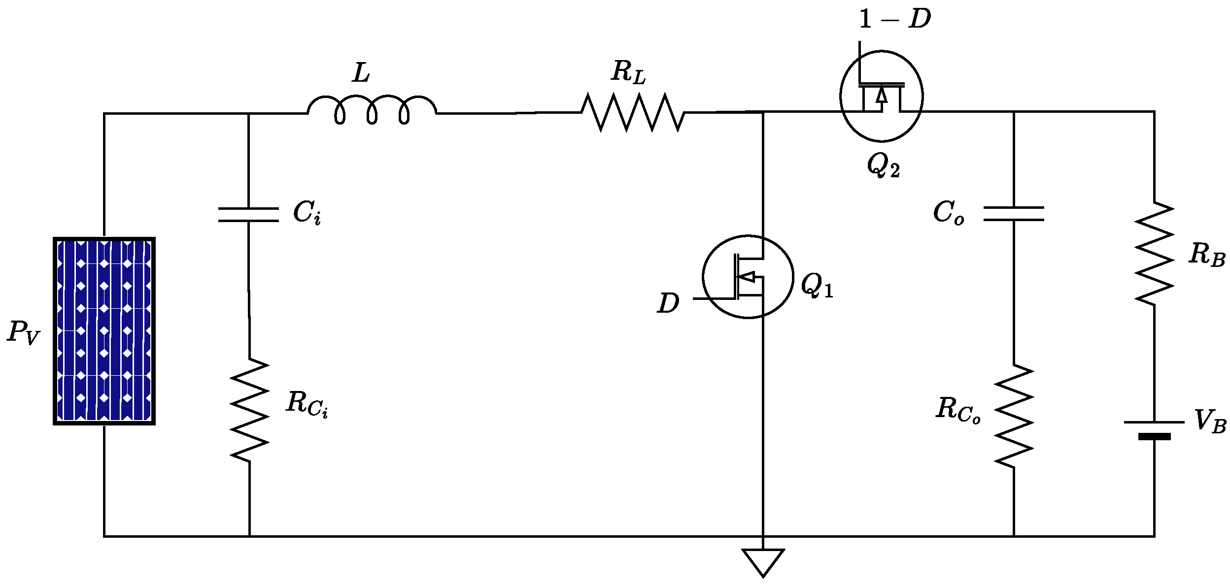
Figure 3.
Estado de activacion del convertidor boost encendido y apagado
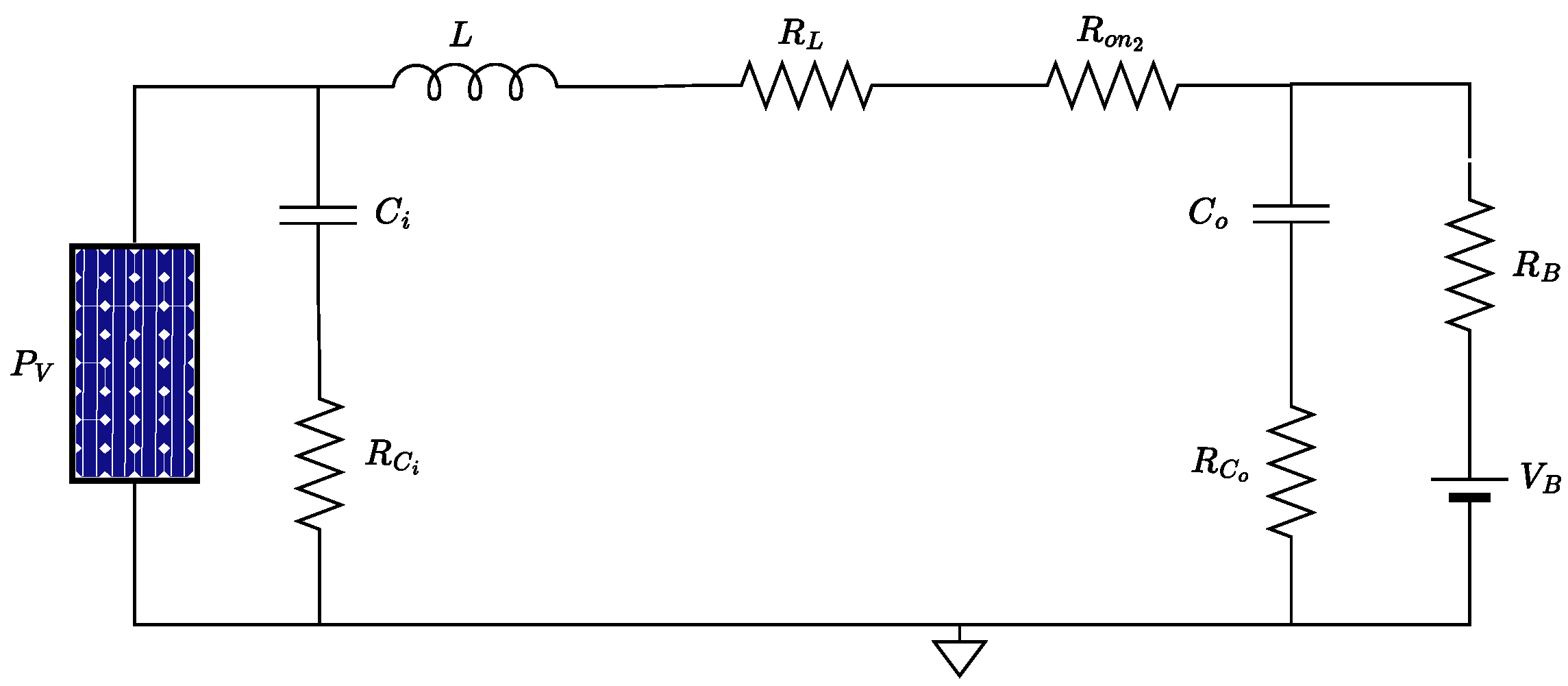
Figure 4.
Estado de activacion del convertidor boost apagado y encendido
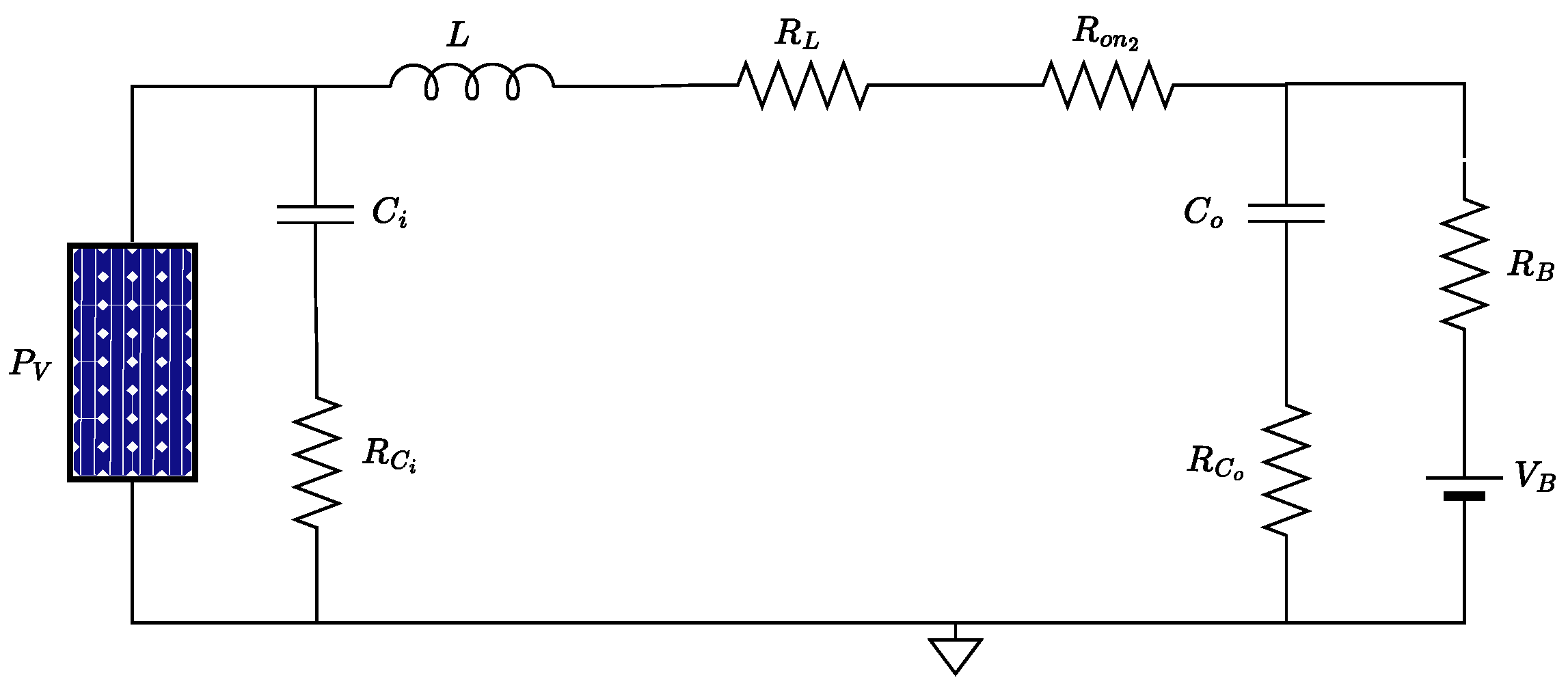
Figure 5.
Perturb and Observe Algorithm Flowchart
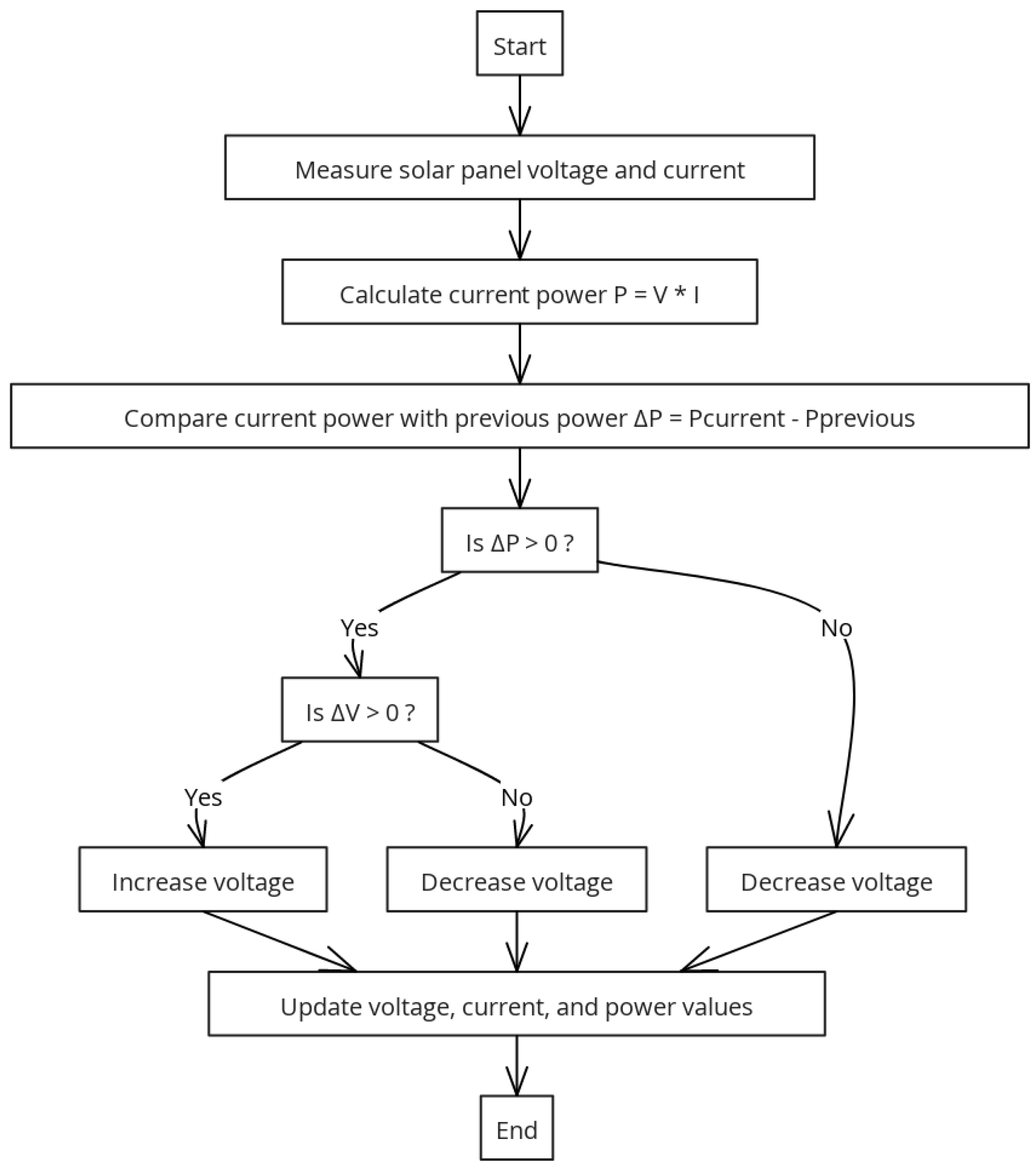
Figure 6.
Incremental Conductance Algorithm Flowchart
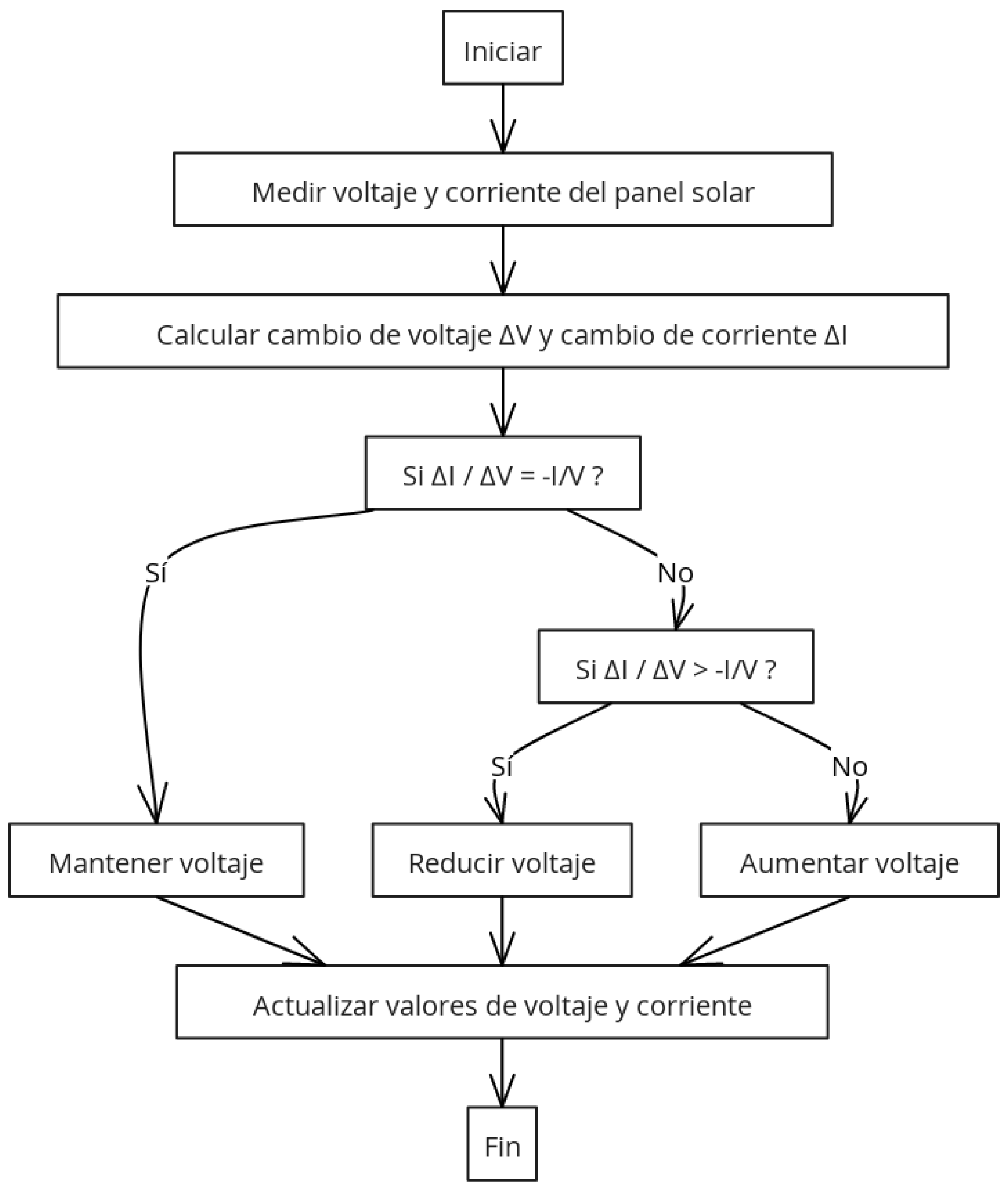
Figure 7.
Experimental Simulink configuration used to validate the results.
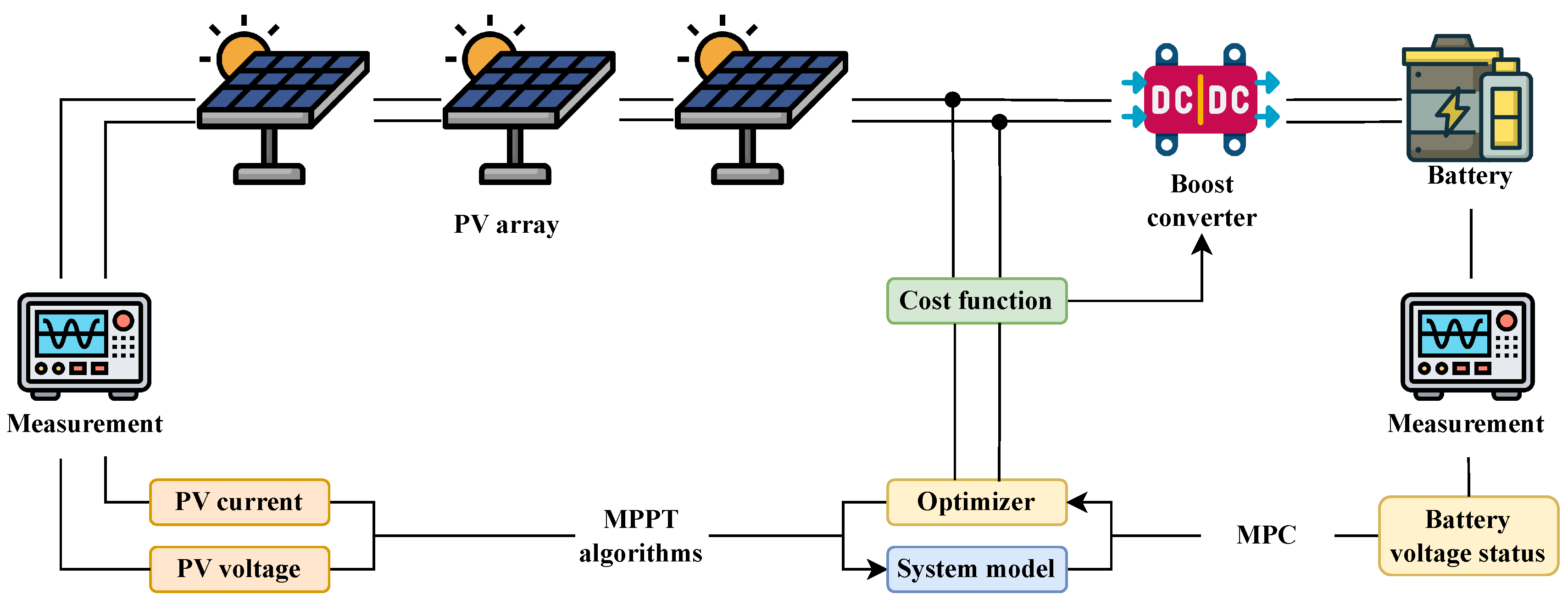
Figure 8.
Comparison between the traditional Incremental Conductance algorithm and the proposed improved algorithm.
Figure 8.
Comparison between the traditional Incremental Conductance algorithm and the proposed improved algorithm.
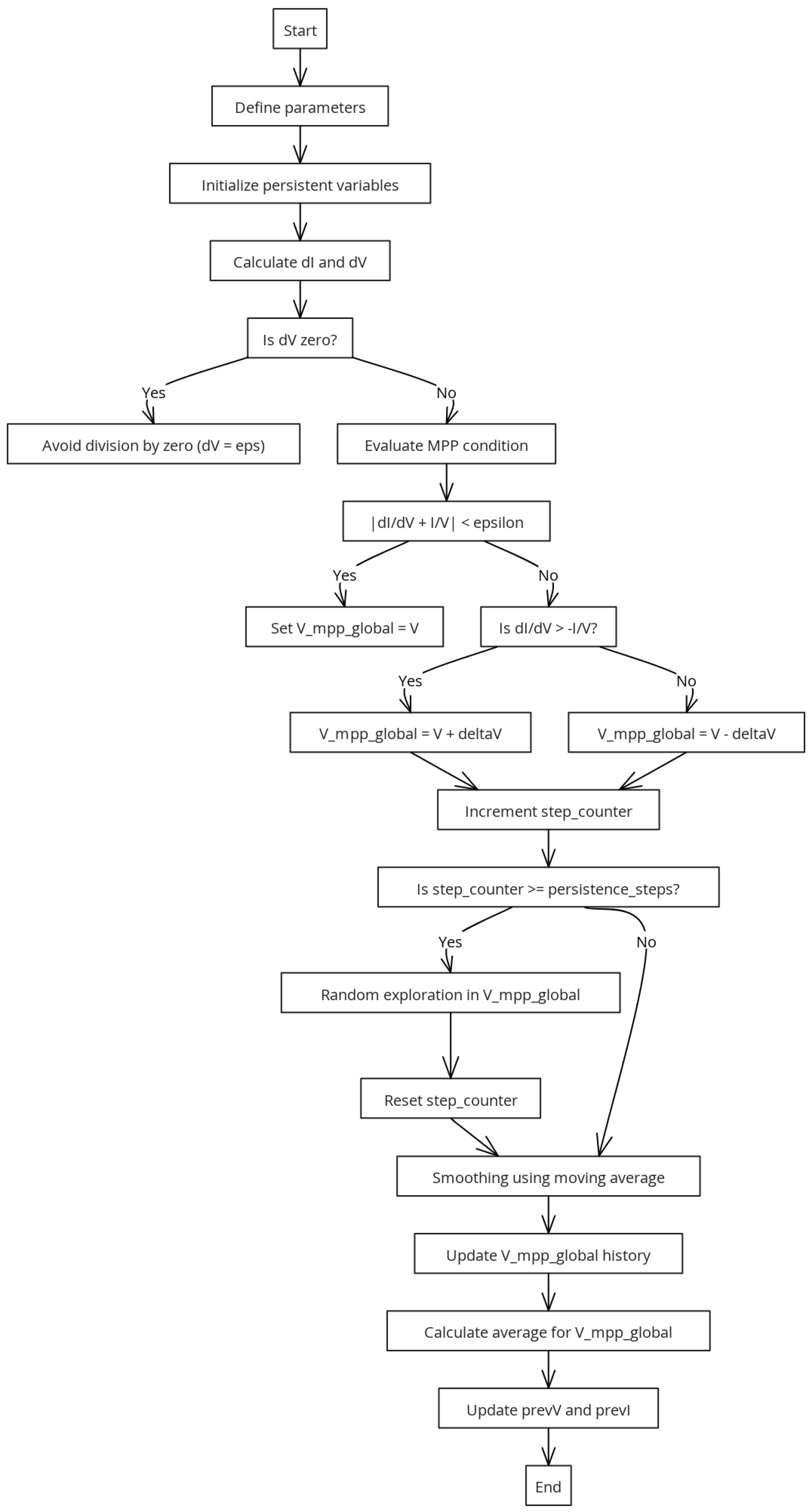
Figure 9.
Matlab/Simulink model used to validate the nonlinear MPC controller and the enhanced Incremental Conductance algorithm.
Figure 9.
Matlab/Simulink model used to validate the nonlinear MPC controller and the enhanced Incremental Conductance algorithm.
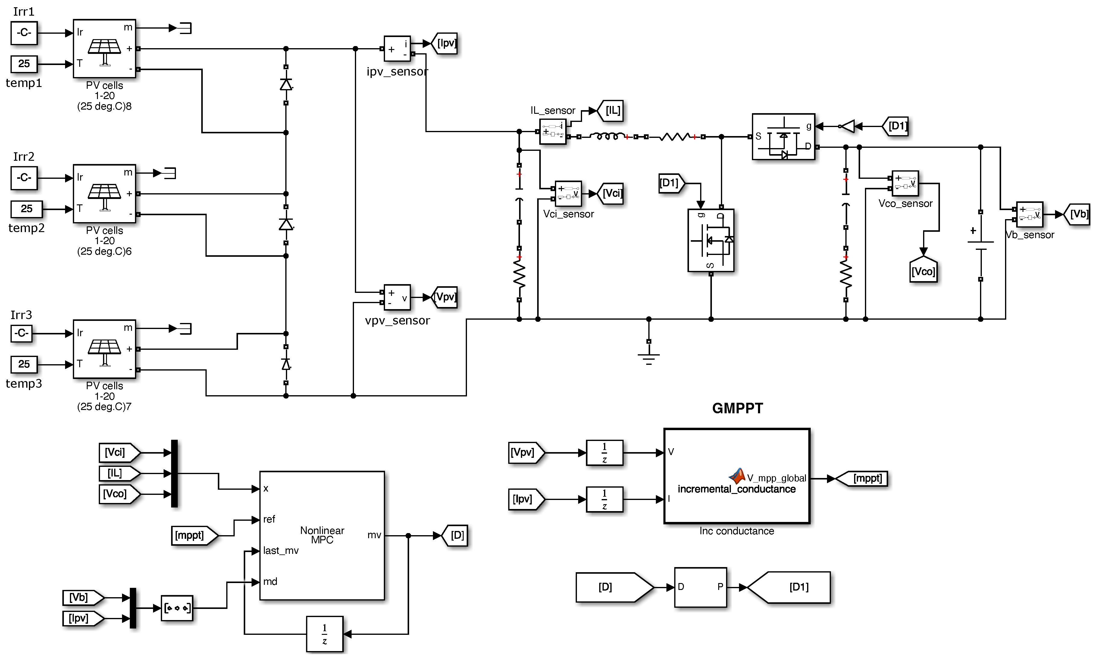
Figure 10.
System results under irradiance conditions of 1000, 300, and 600 .
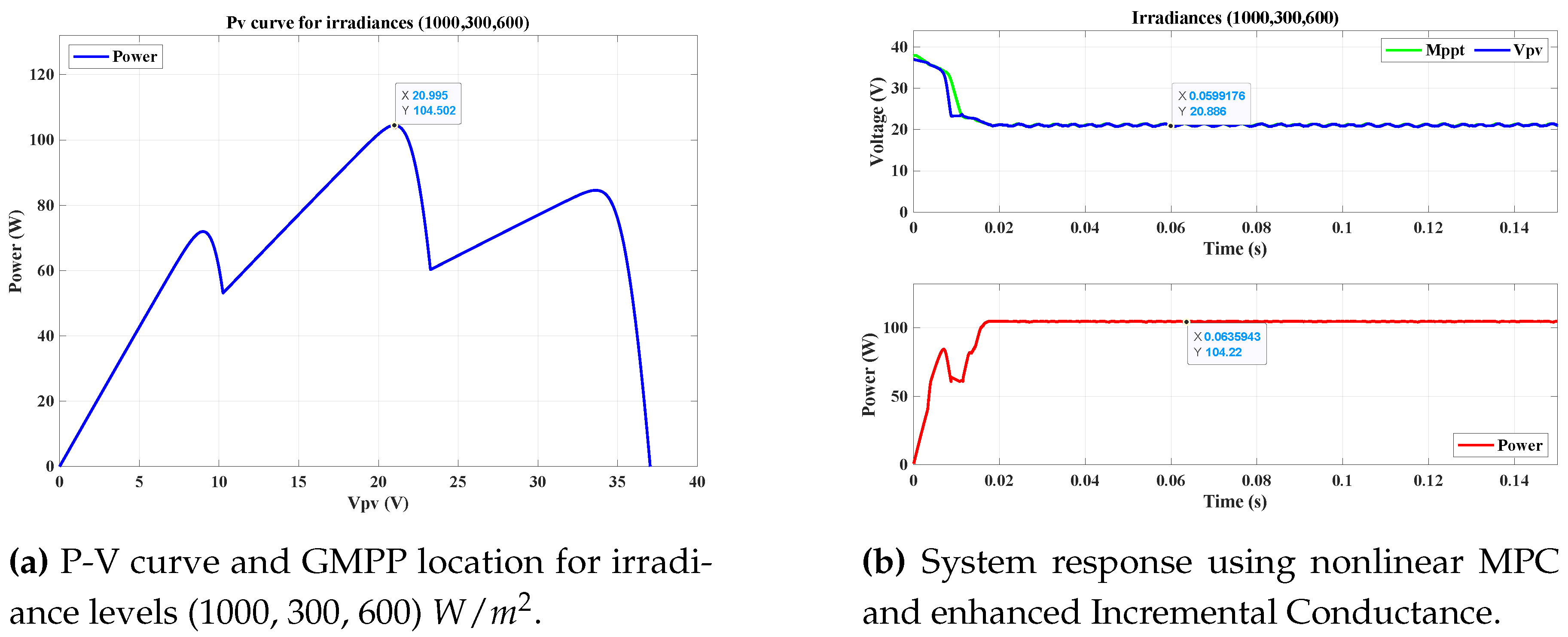
Figure 11.
System results under irradiance conditions of 500, 300, and 600 .
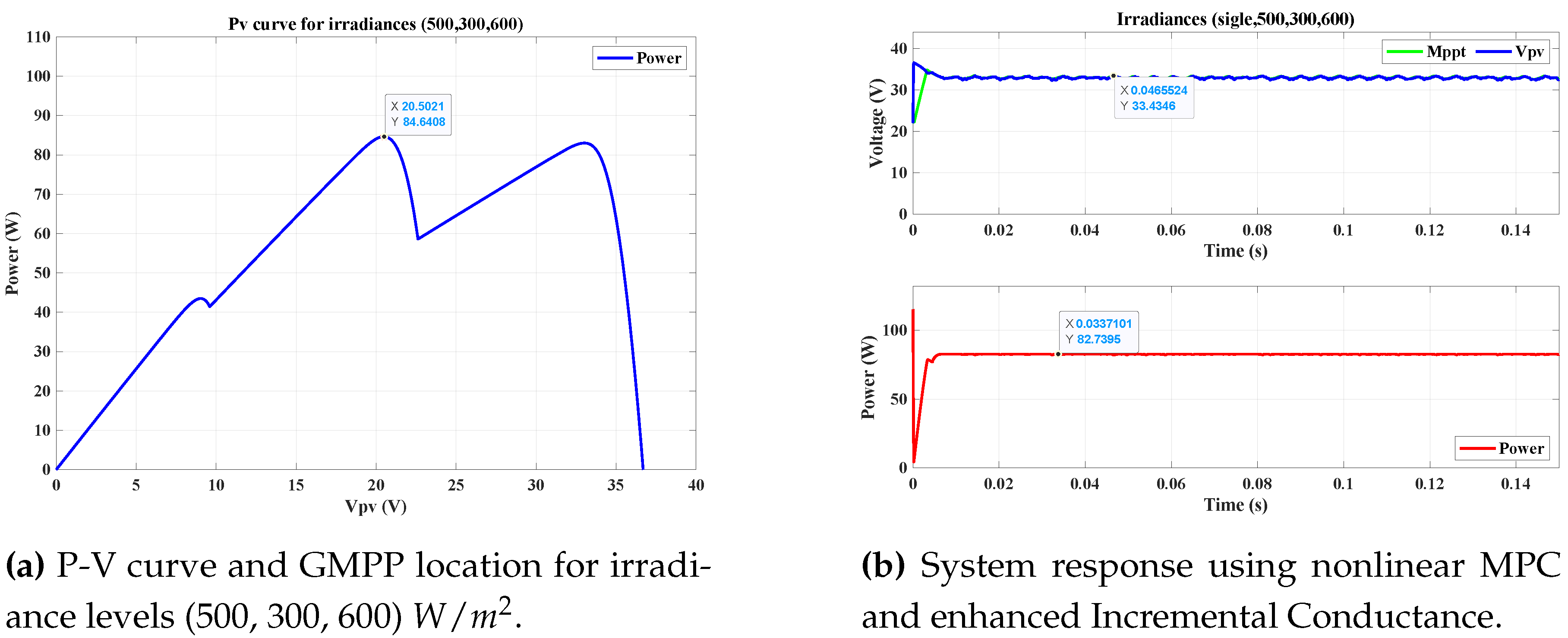
Figure 12.
System results under irradiance conditions of 500, 1000, and 600 .
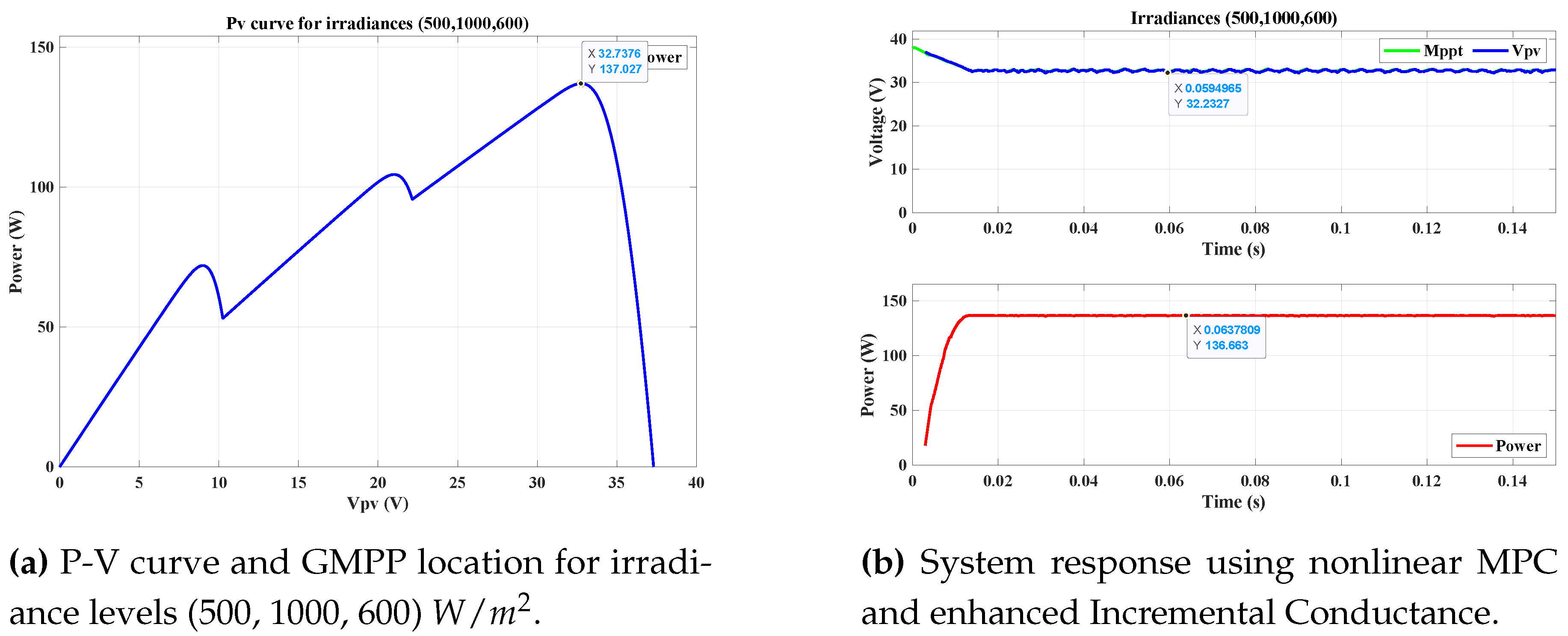
Figure 13.
System results under irradiance conditions of 500, 1000, and 1000 .
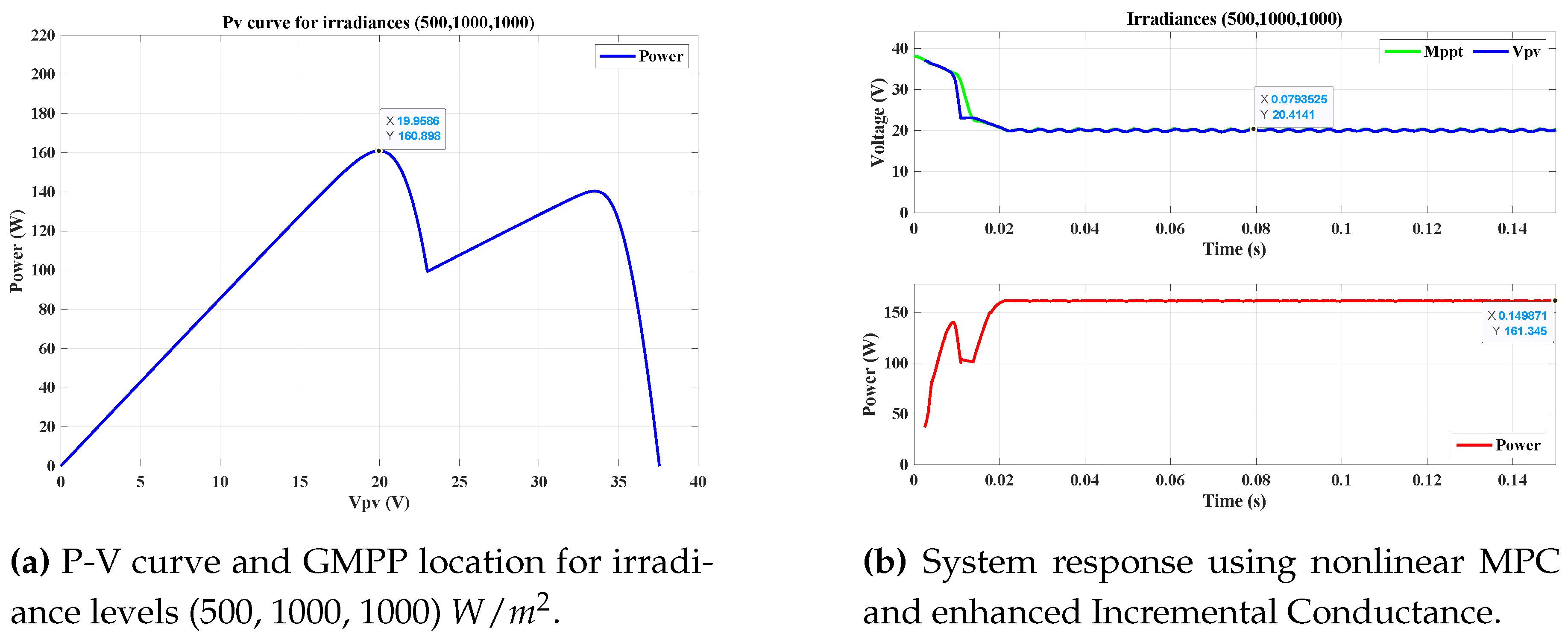
Figure 14.
System results under irradiance conditions of 300, 1000, and 400 .
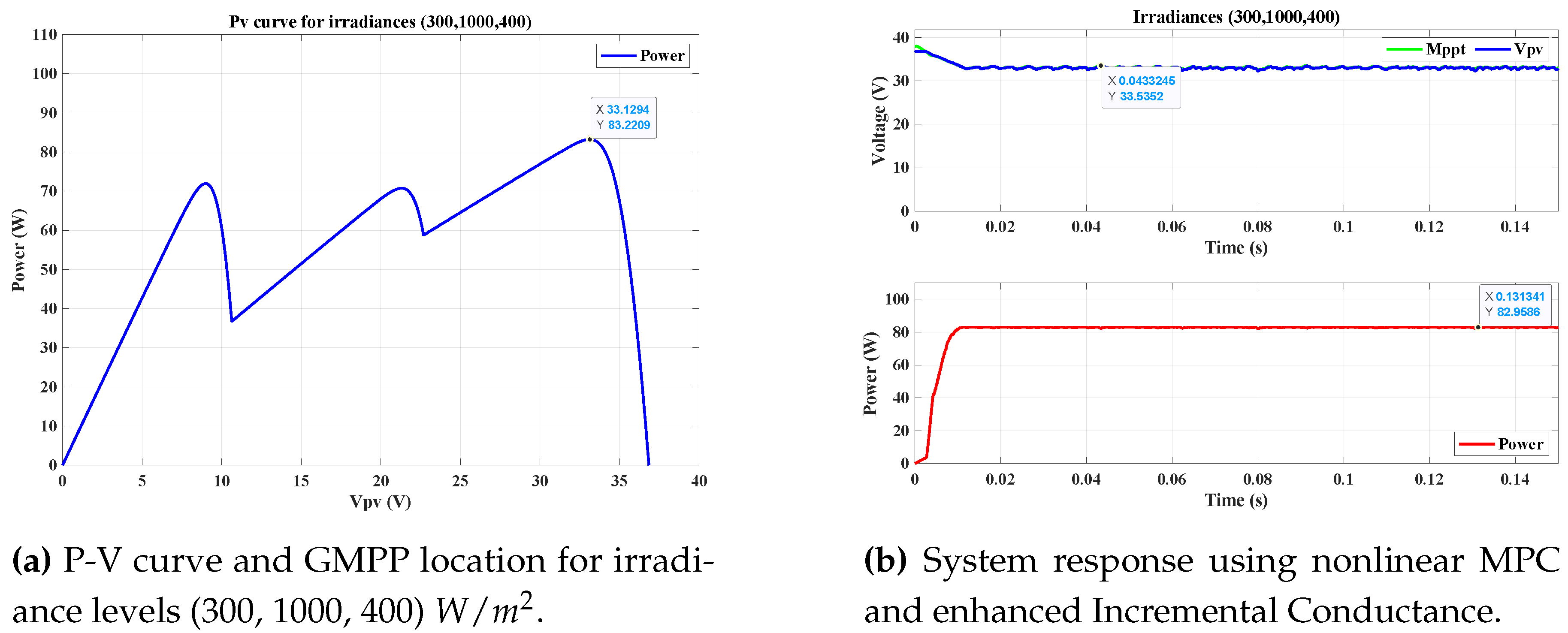

Table 1.
Test system parameters and specifications.
| Parameter | Symbol | Value |
|---|---|---|
| Solar Panel Parameters at STC | ||
| Maximum power | 83.28 W | |
| Voltage at | 10.32 V | |
| Current at | 8.07 A | |
| Short-circuit current | 8.62 A | |
| Open-circuit voltage | 12.64 V | |
| Temperature coefficient of | 0.063%/°C | |
| Temperature coefficient of voltage | -0.33 mV/°C | |
| Converter Parameters | ||
| Input capacitor | 22 F | |
| Output capacitor | 22 F | |
| Inductor | L | 330 H |
| Inductor resistance | 60 m | |
| ON resistance Mosfet 1 | 35 m | |
| ON resistance Mosfet 2 | 35 m | |
| DC Load Parameters | ||
| DC load equivalent resistance | 60 m | |
| DC load voltage | 24 V | |
Table 2.
Parameters of the Nonlinear MPC Controller for the Boost Converter.
| Parameter | Value |
|---|---|
| Prediction horizon | 2 |
| Control horizon | 1 |
| Lower limit of duty cycle | 0 |
| Upper limit of duty cycle | 1 |
| Sampling frequency () | s |
Table 3.
Irradiance values assigned to each PV panel for the defined scenarios.
| Scenario | Irradiance PV1 | Irradiance PV2 | Irradiance PV3 | Expected Power (W) |
|---|---|---|---|---|
| 1 | 1000 | 300 | 600 | 104.5 |
| 2 | 500 | 300 | 600 | 84.64 |
| 3 | 500 | 1000 | 600 | 137.0 |
| 4 | 500 | 1000 | 1000 | 160.9 |
| 5 | 300 | 1000 | 400 | 83.22 |
Disclaimer/Publisher’s Note: The statements, opinions and data contained in all publications are solely those of the individual author(s) and contributor(s) and not of MDPI and/or the editor(s). MDPI and/or the editor(s) disclaim responsibility for any injury to people or property resulting from any ideas, methods, instructions or products referred to in the content. |
© 2025 by the authors. Licensee MDPI, Basel, Switzerland. This article is an open access article distributed under the terms and conditions of the Creative Commons Attribution (CC BY) license (http://creativecommons.org/licenses/by/4.0/).
Copyright: This open access article is published under a Creative Commons CC BY 4.0 license, which permit the free download, distribution, and reuse, provided that the author and preprint are cited in any reuse.


