Chaotic Transitions and the Origin of Spacetime: An Analysis Based on the Lorenz Model

1. Introduction

The study of chaos and order, fundamental themes for understanding the universe, plays a crucial role in physics, especially when analyzing complex nonlinear systems such as the Lorenz model. In Chaos and Order: The Foundation of Spacetime’s Origin, we discuss how these two forces seem intrinsic to the fundamental structure of reality. In this context, the chaotic behavior of these systems is not merely a manifestation of fluctuations but a key to understanding the transitions that may give rise to the very fabric of spacetime. Building on this foundation, this work aims to deepen the analysis of these chaotic transitions and how they may offer new insights into the origin and nature of spacetime, suggesting that it may indeed have emerged from a primordial state of chaos. Using the Lorenz model as a mathematical analogy, we explore how order and chaos can interlace, offering a clearer view of the dynamics underlying our reality.

2. Methodology

2.1. The Lorenz Model

The Lorenz model is a system of differential equations that describes thermal convection in a fluid. It is governed by three parameters: σ (Prandtl number), β (geometrical aspect of the fluid), and ρ (heat source ratio). The system’s equations are:

$${\displaystyle \frac{\mathit{d}\mathit{x}}{\mathit{d}\mathit{t}}}=\mathit{\sigma }\left(\mathit{y}-\mathit{x}\right)$$

$${\displaystyle \frac{\mathit{d}\mathit{y}}{\mathit{d}\mathit{t}}}=\mathit{x}\left(\mathit{\rho }-\mathit{z}\right)-\mathit{y}$$

$${\displaystyle \frac{\mathit{d}\mathit{z}}{\mathit{d}\mathit{t}}}=\mathit{x}\mathit{y}-\mathit{\beta }\mathit{z}$$

These equations, typical in nonlinear dynamical systems, describe the evolution of the system over time, capturing the interaction of various variables that affect the system’s behavior. The ρ parameter, known as the control or bifurcation parameter, determines the system’s sensitivity to initial conditions and can significantly influence its dynamics.

As the value of ρ increases, the system undergoes a series of transitions, starting from predictable, stable behavior with periodic solutions to more complex and unpredictable behavior. When ρ reaches a critical value, known as the bifurcation point, the system ceases to be deterministic and enters a chaotic regime. At this point, small variations in initial conditions can lead to completely different trajectories, making long-term prediction of the system’s behavior impossible. Chaos is characterized by its high sensitivity to initial conditions, meaning that the system becomes extremely sensitive to even the slightest variation, amplifying these differences over time.

This critical point, where the system transitions from regular to chaotic behavior, is of great importance for understanding dynamical systems found in physics, biology, and other fields. In many cases, chaos is not entirely random but follows complex, often fractal patterns, showing that even in chaotic systems, there is an underlying order that can be analyzed through mathematical and computational methods.

3. Results

3.1. Behavioral Transition in the Lorenz Model

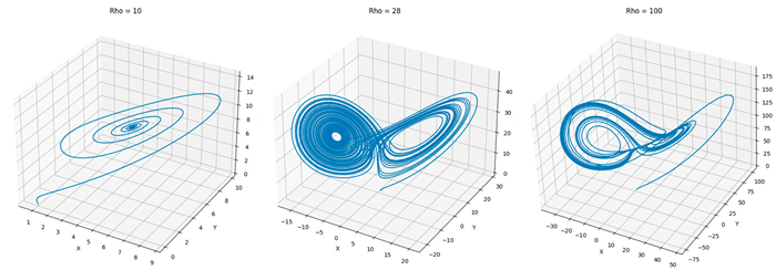
A key feature of the Lorenz system is its sensitive dependence on parameters. Variation in the ρ parameter (Rayleigh number) leads to different dynamic regimes, from stable states to chaotic behavior. Below, we explore this transition with three distinct values of ρ:

• ρ = 10: The system evolves to a fixed point, where trajectories converge to a stable state without exhibiting chaotic behavior.
• ρ = 28: This is the classic value for the chaotic regime, where the system shows the characteristic strange attractor, exhibiting extreme sensitivity to initial conditions.
• ρ = 100: The increase in the parameter alters the attractor’s structure, leading to a more dispersed and less defined chaotic behavior.

The transition between these regimes can be visualized through the evolution of trajectories in phase space, illustrating how small changes in ρ impact the system’s dynamics.

Mathematical Analysis of Chaotic Behavior for ρ=100.

When ρ reaches higher values, such as ρ=100, the system deviates significantly from the behavior observed at lower ρ values. In the chaotic regime, the system’s solutions no longer follow predictable trajectories and can spread unpredictably across phase space.

For a more rigorous analysis of this transition, it would be interesting to study the system’s behavior in terms of Lyapunov dependence, which quantifies the rate of divergence of initial solutions along nearby trajectories. Furthermore, the bifurcation of the system as ρ varies can be used to characterize this change in behavior and identify the exact transition point.

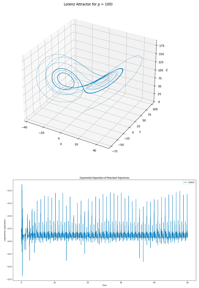
Lyapunov Exponent Analysis.

In the chaotic regime, sensitivity to initial conditions is a hallmark feature. The calculation of the largest Lyapunov exponent allows quantifying this sensitivity. A practical way to estimate the exponent is:

• Evolve a base trajectory and a "perturbed" trajectory (initially separated by a distance $d_0$).
• Measure the separation between the trajectories at regular intervals and re-normalize the difference vector to maintain the initial separation $d_0$.
• Accumulate the stretching factors and compute, at the end, the average of the logarithm of these factors divided by the total time.

A positive value of the largest Lyapunov exponent confirms the presence of chaos, highlighting the rapid separation of initially close trajectories.

Conclusion

The simulation of the Lorenz system with ρ=100 shows that as the parameter is increased, the system moves away from periodic or quasi-periodic behavior observed at lower ρ values. The calculation of the Lyapunov exponent provides a quantitative tool to characterize this transition and reinforces the unpredictable nature of chaotic systems.

Mathematically, chaotic behavior for ρ=100 is largely associated with the exponential divergence of trajectories, which is a fundamental characteristic of chaotic systems. However, this transition may be more complex than simply an abrupt change. The transition between regimes can be gradual, with the system passing through intermediate states of pseudo-chaotic behavior before reaching full chaos.

The Lorenz system, widely studied in dynamical systems, exhibits chaotic behavior characterized by high sensitivity to initial conditions. The equations describing it depend on three fundamental parameters: σ, ρ, and β, with ρ playing a crucial role in the transition between regular and chaotic regimes. In systems like this, small variations in parameters can result in drastic changes in the system’s behavior.

As ρ increases, the system undergoes a transition where regular dynamics transform into chaotic behavior. The critical value of ρ=100 represents a significant change in this behavior. However, the nature of this transition—whether gradual or abrupt—depends on several factors, including initial conditions and potential disturbances affecting the system.

3.2. Effect of External Perturbations on the Lorenz System

In this section, we analyze how external perturbations affect the Lorenz system’s behavior. We compare the evolution of the system in two scenarios: one without external disturbances and another with a periodic perturbation applied to the ẋ equation. The perturbation is modeled as a sinusoidal term, representing an external influence that varies over time.

The modified equation for the y parameter is:

$${\displaystyle \frac{\mathit{d}\mathit{x}}{\mathit{d}\mathit{t}}}=\mathit{\sigma }\left(\mathit{y}-\mathit{x}\right)$$

$${\displaystyle \frac{\mathit{d}\mathit{y}}{\mathit{d}\mathit{t}}}=\mathit{x}\left(\mathit{\rho }-\mathit{z}\right)-\mathit{y}+\mathit{sin}\mathit{s}\mathit{i}\mathit{n}\left(2\mathit{\pi }\mathit{f}\mathit{t}\right)$$

$${\displaystyle \frac{\mathit{d}\mathit{z}}{\mathit{d}\mathit{t}}}=\mathit{x}\mathit{y}-\mathit{\beta }\mathit{z}$$

where A represents the amplitude of the external perturbation, f is the frequency of the disturbance, and sin(2πft) models the periodic oscillation over time. This additional term in the ẏ equation simulates an external perturbation that can alter the system’s behavior, inducing, for example, an oscillatory effect or even more pronounced chaotic behavior depending on the parameter values.

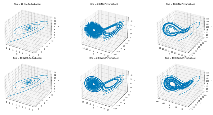
System Without Perturbations.

In the absence of external perturbations, the system follows its natural trajectory, dictated by the parameters σ = 10, β = 8/3, and various values of ρ (10, 28, and 100). As observed in previous analyses, the system exhibits the following behaviors:

• ρ = 10: The system converges to a stable fixed point.
• ρ = 28: The classic chaotic attractor emerges, showing sensitive dependence on initial conditions.
• ρ = 100: The attractor’s structure changes significantly, forming a more complex and elongated trajectory.

System with External Perturbations

The introduction of a periodic perturbation alters the system’s dynamics. The impact of the perturbation depends on its amplitude and frequency. Key observations include:

• For low ρ values (ρ = 10), the system remains close to the fixed point, but small oscillations appear, delaying convergence.
• For ρ = 28, the perturbation increases the unpredictability of the trajectories, amplifying chaotic behavior. The attractor deforms, and transitions between lobes occur more frequently.
• For ρ = 100, the structure becomes even more irregular, and additional instabilities arise, suggesting that the system may be transitioning between different chaotic regimes.

Impact of Disturbances on Chaotic Behavior

When disturbances are introduced into a system, whether through small variations in initial conditions or modifications in parameters, the system’s behavior can be significantly altered. These disturbances can either regularize the system’s behavior or amplify chaos, depending on the nature and magnitude of the alteration.

For example, if the disturbance affects the parameter ρ, the system may oscillate between regular and chaotic states, depending on the intensity of the modification. This leads us to consider that the transition between regimes is not necessarily abrupt but may occur gradually depending on the nature of the disturbances and how they interact with the system.

Moreover, analyzing how small disturbances affect the system’s trajectory can be done using a bifurcation diagram, which allows for the visualization of transitions between different dynamic regimes and the evaluation of solution stability.

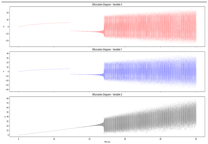
Analysis of Diagrams

• Bifurcation Diagram of X: Initially, the variable X exhibits stable values for small ρ, indicating a fixed point. As ρ increases, successive bifurcations occur, leading to oscillatory behavior and, later, chaos.
• Bifurcation Diagram of Y: The behavior of Y follows a pattern similar to X, with progressive transitions to periodic oscillations and chaos. However, the amplitude of Y’s variations shows subtle differences, reflecting the system’s three-dimensional nature.
• Bifurcation Diagram of Z: The variable Z, associated with the system’s height, also displays an ordered regime for small ρ, followed by nonlinear oscillations and a transition to the chaotic regime. This behavior highlights the system’s sensitivity to initial conditions and changes in parameters.

Conclusion

The bifurcation diagrams reveal the dynamic richness of the Lorenz system. Small variations in the ρ parameter can result in abrupt transitions between ordered and chaotic regimes, highlighting the unpredictability inherent in nonlinear dynamic systems. These findings emphasize the importance of chaos theory in understanding complex natural phenomena, such as meteorology and fluid turbulence.

3.3. Exploring the Impact of σ on the Lorenz System

The σ parameter, representing the rate of heat transfer relative to momentum diffusion in the system, influences the Lorenz system’s sensitivity to initial conditions. In this study, we investigate the effects of low (σ = 5) and high (σ = 20) values of σ, observing how these variations impact the system’s transition to chaotic behavior and the speed at which the system enters this highly sensitive regime.

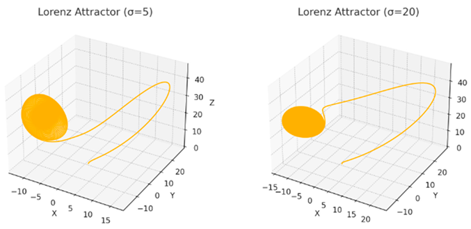
1. σ = 5 - Slower Entry into the Chaotic Regime

For a reduced value of σ, we observe that the system’s trajectories take longer to deviate from the initial conditions and reach chaotic behavior. The attractor formed exhibits a more gradual transition, suggesting that sensitivity to initial conditions increases slowly.

2. σ = 20 - Rapid Transition to Chaos

When σ is increased, the system responds more quickly, entering the chaotic regime in less time. Oscillations grow rapidly, and the separation of trajectories occurs more abruptly, reflecting an increase in sensitivity to initial conditions.

It can be concluded that increasing σ accelerates the transition to the chaotic regime, making the system more unstable more quickly. This effect can be interpreted as an intensification of the system’s nonlinearity, where small variations in initial conditions result in drastically different trajectories in less time.

3.4. Connection with Chaos Theory

We can use the analogy of the σ parameter to describe how, at the origin of the universe, fluctuations were “exaggeratedly high,” meaning the system was in an extremely sensitive and chaotic regime. As the universe expanded and cooled, these fluctuations decreased, leading to greater stability and the formation of the structures we observe today, such as galaxies, stars, and planets.

These points can be related to the concept of a transition from primordial "chaos" to "emergent order," an interesting and coherent analogy with the behavior of chaotic systems.

4. Formation of Structures in the Universe: An Analogy with Chaotic Systems

Chaotic behavior, especially in nonlinear dynamic systems like the Lorenz system, has interesting parallels with the formation of structures in the universe. Chaos often leads to self-organization and the creation of complex patterns, a phenomenon observed in various physical systems, including the formation of galaxies and stars.

When thinking about the evolution of the universe, we can envision a process where, starting from highly disordered initial conditions, organizational patterns emerge, such as the structures we see in the cosmos. The self-organizing nature of chaos in systems like Lorenz can serve as a mathematical analogy for understanding how structures in the universe form, despite the underlying chaotic dynamics.

This self-organizing behavior in the context of chaos should not be underestimated, as it is a fundamental aspect that can explain how seemingly disordered systems can generate regularities and organized patterns. In many ways, chaos and order are not mutually exclusive but complementary aspects of the same reality, as seen in the formation of stars or even in complex biological systems.

5. Relationship Between Chaos, Cosmology, Big Bang, and Conclusions

The chaotic dynamics of the Lorenz model offer an interesting analogy for understanding the origin of space-time. The Big Bang, often described as a singular and highly unstable event, can be interpreted as a transition from a primordial chaotic state to subsequent organization. Just as in the Lorenz model, where small disturbances in initial conditions result in completely different trajectories, quantum fluctuations in the primordial universe played a crucial role in the formation of the structures we observe today.

The transition between ordered and chaotic states can be mathematically analyzed through the Lorenz system’s bifurcation diagram. This diagram illustrates how small variations in the control parameter (ρ) cause abrupt changes in the system’s behavior. Similarly, in the cosmological context, factors such as energy density and vacuum fluctuations determined the transition from the early universe to a more structured state, leading to the formation of galaxies and other cosmic structures.

Additionally, the analysis of Lyapunov exponents, which measures the system’s sensitivity to initial conditions, can be applied to understanding the process of cosmic inflation. During inflation, small fluctuations were exponentially amplified, giving rise to the anisotropies observed in the cosmic microwave background radiation and the distribution of matter in the universe. This relationship between chaos and cosmological expansion suggests that chaotic dynamics may have played a fundamental role in the early structuring of space-time.

Thus, the analogy between chaotic dynamic systems and the evolution of the universe not only provides a fresh perspective on the transition between chaos and order but also reinforces the idea that the laws of chaos may be deeply intertwined with the very origin of space-time.

References

- Lorenz, E. N. (1963). Deterministic Nonperiodic Flow. Journal of the Atmospheric Sciences, 20(2), 130-141.
- Sprott, J. C. (2003). Chaos and Time-Series Analysis. Oxford University Press. [CrossRef]
- Hawking, S. (1988). A Brief History of Time. Bantam Books.
- Penrose, R. (2004). The Road to Reality: A Complete Guide to the Laws of the Universe, Alfred A. Knopf.
- Strogatz, S. H. (2015). Nonlinear Dynamics and Chaos: With Applications to Physics, Biology, Chemistry, and Engineering. Westview Press.
- Gleick, J. (1987). Chaos: Making a New Science. Viking.
- Ott, E. (2002). Chaos in Dynamical Systems. Cambridge University Press.
- Cvitanović, P. (2017). Chaos: Classical and Quantum. Niels Bohr Institute.
- Peitgen, H.-O., Jürgens, H., & Saupe, D. (2004). Chaos and Fractals: New Frontiers of Science. Springer.
Disclaimer/Publisher’s Note: The statements, opinions and data contained in all publications are solely those of the individual author(s) and contributor(s) and not of MDPI and/or the editor(s). MDPI and/or the editor(s) disclaim responsibility for any injury to people or property resulting from any ideas, methods, instructions or products referred to in the content. |
© 2025 by the authors. Licensee MDPI, Basel, Switzerland. This article is an open access article distributed under the terms and conditions of the Creative Commons Attribution (CC BY) license (http://creativecommons.org/licenses/by/4.0/).
Copyright: This open access article is published under a Creative Commons CC BY 4.0 license, which permit the free download, distribution, and reuse, provided that the author and preprint are cited in any reuse.