Submitted:
24 June 2025
Posted:
24 June 2025
You are already at the latest version
Abstract
Limited fossil fuels have created a societal energy crisis necessitating the use of renewable energy. However, existing renewable energy sources are problematic and incur high costs. To solve these problems, we propose a new renewable energy source with a divergent current density and highly symmetric circuits. When starting the circuit, we calculated the large current to be harvested and the output electric power. During our experiments, a significantly large divergent current flowed into a huge resistance, boosting the output electric power to a level almost equal to that of a nuclear power station. In addition, the experimental results were consistent with the theoretical expectations.
Keywords:
applied physics
; renewable energy
; higly symmetric circuit
; stray capacitor
; paired‐light‐emitting diodes
; paired‐DC‐motor
; divergent current density
; electric power
1. Introduction
The depletion of fossil fuels such as crude oil and
natural gas has created societal energy problems. Moreover, the limited
availability of high-cost crude oil has caused economic problems. To mitigate
these concerns, countries are attempting to introduce renewable energies [1–6], but such alternatives cannot (in most cases)
satisfy 100% of the demand. Moreover, most renewable energies fluctuate with
natural climate variations, complicating the system, planning, and control
methods [7]. The most promising of the
existing renewable energies are solar and wind power [8,9]
but they require high costs as will be described. Furthermore, fossil fuel
consumption is a cause of rising CO2 concentration [10,11]. The spread of renewable energy sources must
be considered from both economic and technological perspectives. Highly
efficient, low-cost energy generation is of major importance [12,13].
To reduce the atmospheric CO2 concentration,
existing renewable energy sources such as solar and wind power must be widely
adopted. However, the integration of renewable energy into the existing power
systems risks frequency and voltage disruptions. Moreover, effective
performance from the existing energy sources requires many expensive storage
batteries.
Japan has declared a goal of net-zero carbon by
2050, but simulations [14,15] have shown that
meeting this goal might be impossible without breakthrough technologies.
The main problems with the existing renewable
energy and nuclear power generation are summarized below.
- 1)
- Renewable energy sources depend on the weather, necessitating large and expensive storage batteries. Moreover, introducing renewable energy sources to the existing energy systems will destabilize the outputs.
- 2)
- Simulations assessing the possibility of achieving net-zero carbon in Japan have included nuclear power generation [16] without considering its dangers. For instance, the Fukushima nuclear accident in Japan in 2011 caused extensive damage.
- 3)
To solve the above problems, this paper proposes a
new system for stable energy production meeting the demands of Japan, i.e., the
required amount of energy in the right place at the right time. Moreover, our
system is highly efficient with low costs.
Our previously proposed energy-generating system [18,19] could not generate sufficiently large
amounts of energy, although they could provide stable energies. The present
paper proposes a new concept for generating a large amount of renewable energy
using a highly symmetric circuit with significantly low costs. When certain
conditions are satisfied, the circuit provides an apparent divergent current
with no Joule heating to both paired light-emitting diodes (LEDs) and paired
direct current (DC) motors, boosting the electric power. This power-generation
phenomenon is verified in both theory and experiments. We discuss the good
agreement between the theory and experiments, and will describe whether the
results satisfy the purpose and motivation of this study.
2. Materials and Methods
Figure 1 is a
schematic of the presented model near its initial state. The circuit employs
two same-output voltage sources V and two identical loads which are not pure
electrical loads, as they must output an energy of Eout per
electron. As shown in the figure, this circuit system is highly symmetric. The
voltage (V) is expressed in terms of the electric potential (φe) as follows:
Figure 1.
Circuit configuration near the initial state, consisting of identical loads (blue blocks) that must output an energy of Eout per electron. Note that φe is the electric potential, and then α, β, α’, and β’ are taps. Moreover, V is the output of a voltage source.
Figure 1.
Circuit configuration near the initial state, consisting of identical loads (blue blocks) that must output an energy of Eout per electron. Note that φe is the electric potential, and then α, β, α’, and β’ are taps. Moreover, V is the output of a voltage source.
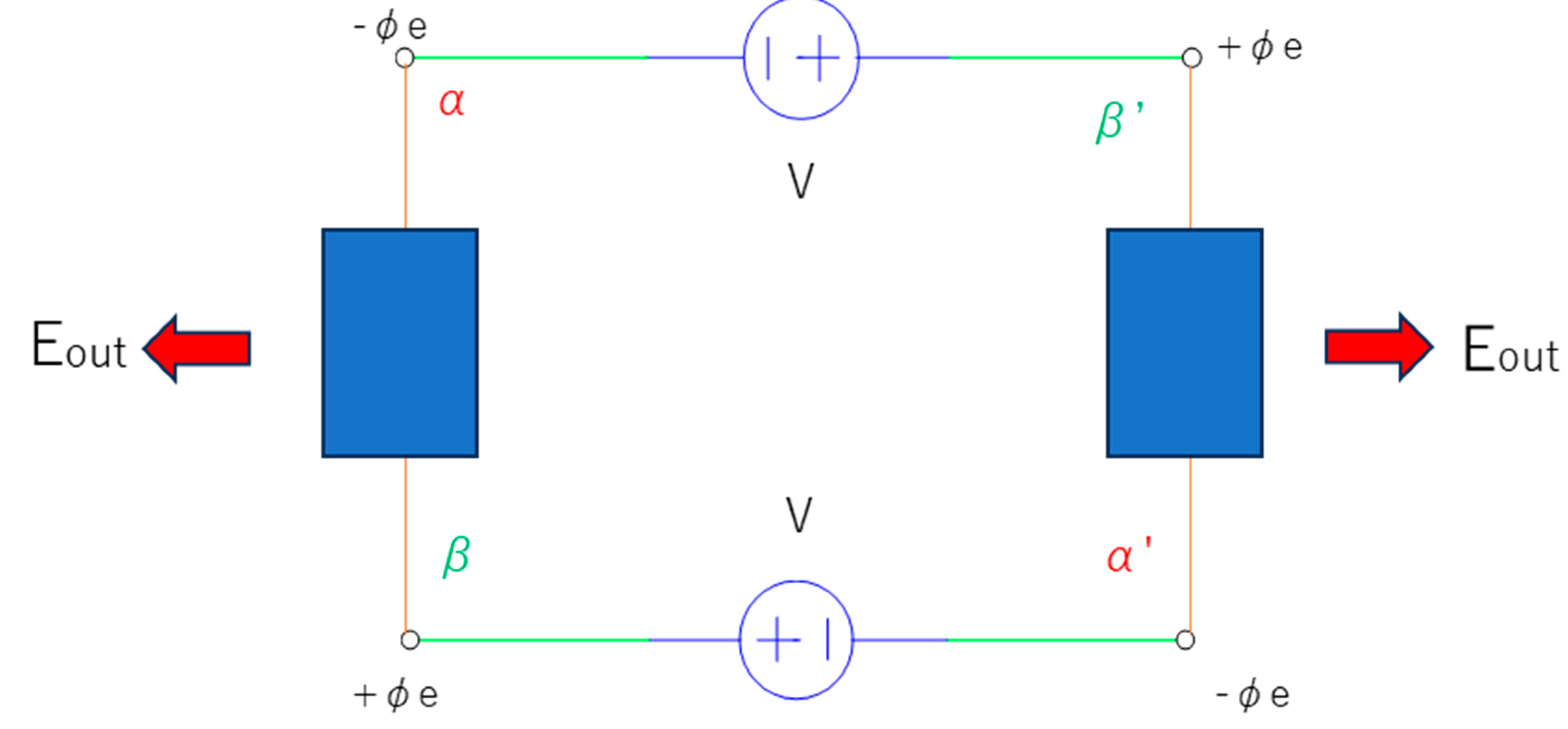
Note that α, β, α’
and β’ in Figure 1 are
the names of taps.
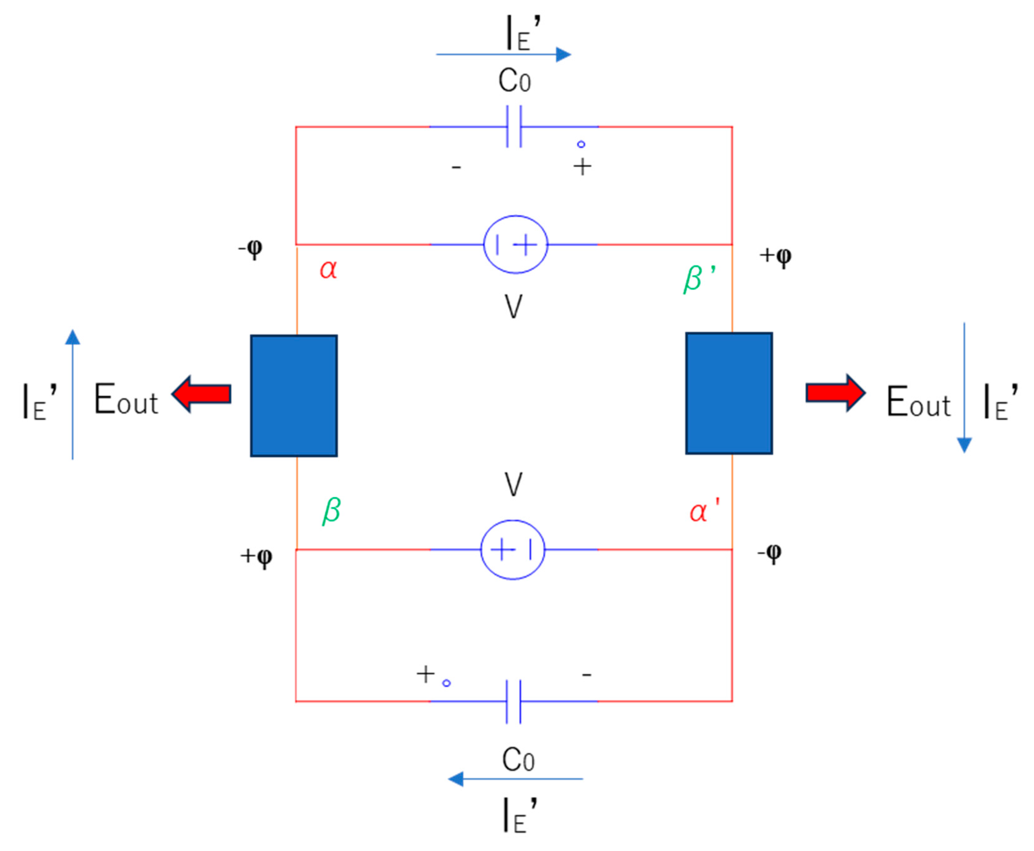
The principle of the model is shown in Figure 2, which (unlike Figure 1) includes a pair of stray capacitors C0
embedded in a vacuum. At initial time t = 0, the stray condensers C0
are shorted. (Note that a condenser is generally shorted at the initial
state due to its voltage–current characteristic.) Moreover, completely at t=0,
the loads do not output the energies due to no current because the stary
condenser C0 are shorted and thus at t=0, all the currents in
the system are distributed to the stray condenser C0. At some
transition time t = tc, which is essentially equal to
the time constant () (i.e., the product of the capacitance (C0)
and load resistance (R) of the load), there is a transient
current (i) in the loads and an emergent
electric potential (φ) defined as follows:
where e is the electron charge.
Figure 2.
Schematic at the transition time tc with stray capacitors C0. The paired condensers repetitively store and discharge energy, generating a constant current
Figure 2.
Schematic at the transition time tc with stray capacitors C0. The paired condensers repetitively store and discharge energy, generating a constant current

. The voltage sources V in this state are dead
apart from momentary activity near the initial state. Note that α, β, α’,
and β’ are taps. Moreover, Eout is the output energy per
electron from a load.
At time (tc), considering the
above definition of the emergent electric potential (φ), the following
condition must be satisfied:
The right-hand side of this inequality indirectly
defines the energy of the voltage source V, which essentially equals to the
Joule heating. The coefficient “2” in the left-side implies that there are two
condensers. Note that, the resistance (R) is the net one including the
loads, lead and contact resistances. Thus, for an electron, we can rewrite the
condition (3) as:
where kB and T denote the
Boltzmann constant and temperature, respectively. Note that both the sides of
inequality (4) imply the avarage energy of an electron.The left-side implies a
work which an electron receives from the condenser. In most situations, the
temperature is the room temperature (i.e.) but inequality (4) implies that Joule heating is
ineffective.
As discussed later, the term equals the kinetic energy.
When the above condition is satisfied, the energies
stored in the condensers are discharged, because the energy balance between the
condenser C0 and the voltage source V breaks. Under the
energy-conservation law, energy interchange between the paired up-condenser and
down-condenser in Figure 2 induces a
constant current (IE’) along the C0-load-to-C0-load
loop. Because the condensers C0 are embedded in a vacuum and cannot
be touched, a divergent current (IE’) is
generated. Note that if the inequality is not satisfied, the condensers never
discharge their current but if the inequality is satisfied, the voltage sources
V momentary operate until the condensers begin discharging at time (tc)
and are dormant thereafter, thereby generating energy.
We now discuss the emergent electric potential (φ)after steady-state, In the vicinity of tap α or β at t
= tc, we have:
And
where Ee and Ec0
denote the ohmic and condenser-associated electric fields, respectively.
Note that the vector (ds) aligns
along the direction of (IE’).
Given that the condenser discharges the current at
this time, we have:
Moreover,
However, in the vicinity of a tap, because , we have:
giving rise to
This equation implies that the ohmic voltage is
ineffective. The volatge of the condenser is updated because of the existence
of the left energy of the condition (3). The electric potential is defined as:
with
This emergent electric potential (φ) is
demonstrated in Figure 3. Note that the
electric potential (φ) is not ohmic but a new electric potential of the
stray condenser during time Let us introduce wave function contributing to the
electron motion.
The general form of the Hamiltonian is:
where the first and second terms describe the
center-of-mass motion and the net electron–electron interaction, respectively.
As will be discussed soon, the following assumption holds:
Moerover, as will be described, assuming that the
scalar is distributed along x-axis and provides
the center-of- mass motion that is equal to the kinetic energy, this scalar
results in a relatively large kinetic energy. Thus, the rest momenta along the
other dimentions can be neglected. The reason why results in the center-of-mass motion is that it is
a constant and does not depend on relative ordinates. Therefore, one-dimension
motion is allowed. Then, let us consider reason of the formation of the
approxiamtion (14). We can assume a uniform electrical potential (φ) at
tap α or β, implying that each electron has approximately the
same electrical potential (φ) because
whether the potential (φ) is macroscopic or microscopic cannot be
discerned. This implies that, as (φ) cannot coexist with a Coulomb
interaction potential (φM), the Hamiltonian (Heff)
is sufficiently small. Note that the satisfaction of the condition (4) implies
no Joule heating and thus we do not need to consider many electrons’
interaction. That is, one-particle picutre is allowed. Moreover, the condition
(4) also implies that an electron penetrates lattices. Thus, the electron
receives no external forces.
Figure 3.
Schematic showing the distribution of the emergent electric potential φ associated with the output energy Eout. The voltage sources steadily decay.
Figure 3.
Schematic showing the distribution of the emergent electric potential φ associated with the output energy Eout. The voltage sources steadily decay.
The Hamiltonians at tap α are:
,
where m, , and denote the mass of an electron, the Hamiltonian of
up-spin electron, and the Hamiltonian of down-spin electron, respectively. Note
that, due to the symmetry, the Hamiltonians of tap α’ are the
same forms as those of tap α, Eq. (15). Moreover, as discussed, each
Hamiltonian essentially implies one-particle picture.
The exclusion prenciple claims that the energies of
up- and down-spin electrons are the same.
Therefore, we consider degeneracies here.
where k is the wavenumber.
Thus,
Thus, the wavefunctions with each spin are
Note that we employed a delta function as the
egenfunction of the position.
For the case of tap α’ we alter the
correspondence of the first and second terms of Eq. (15).
Note that (j) is the imaginary unit.
Similarly to tap α, tap β satisfies the following Hamiltonians:
From the exclusion principle,
Where
The wave functions of β is:
For the case of tap β’, we alter
the correspondence of the first and second terms of Eq. (20):
The Slater determinant:
In the above equation, the delta functions are
substitued.
Thus,
The first and second terms of the above equation
correspond to the left and right sides of the circuit in Figure 3, respectively. The first and second
terms are considered to be related through the Einstein–Podolosky–Rosen
correlation [20].
Here, we consider only the first term of Eq. (27).
The uncertainty relation gives
Because the momentum (p) is
constant as (, the uncertainty becomes infinite, defying the classical physical
motion of an electron from one tap to the other. The wavefunction of the left
part of the circuit is:
The probability density (jE) of
the flow:
is solved as:
Herein, we separately consider paired LEDs or paired DC motors as the loads.
DC motor loads
From the normalization condition:
we have
where λ is the wavelength of an electron.
The wavenumber (k) is defined as:
Thus,
The wavenumber is also derived as:
from which the flow probability density (jE) is obtained as:
That is,
To obtain the net current density [A/m2], we multiply Eq. (37) by the electronic charge (e):
Here, the area (Si) is considered as a unit cell; for example,
Importantly, the net observed current is then derived as:
LED loads
Under the normalization condition:
The photon imparts its momentum to an electron and hole and thus the wave number of a carrier becomes a half of Eq. (43), considering the conservation of the momentum.
And
Similarly to the DC motor, the LED loads obtain a net current density of:
As the net current is contributed by an electron and a hole, we have:
Within the area (Si) of a unit cell, e.g.,
the net current is
Next, the DC-motor loads must satisfy two conditions. Let us consider these conditions:
The general motion equation of a motor is [22] as follows:
where Ra [Ω], Ia [A], L [H], and E [V] denote the inner resistance, working current, inductance, and reverse electromotive force, respectively.
Let us first obtain the general solution from Eq. (50). To obtain this solution, setting the nonhomogeneous term to zero, the general solution is immediately obtained as:
At completely t = 0 when all currents flow into the condensers C0 in our system, the initial current in the motor is zero; that is:
Moreover, the special solution of Eq. (50) is derived by:
Thus, by the substitution to Eq. (50),
and thus the net solution, i.e., the sum of the general solution and the special solution, is:
The transient equation of the motors in our system is then given by:
Where
In this equation, the proportionality constant (kE) depends on the magnetic flux, and (Ωm) is the rotational velocity.
The current (Ia) is considered as the constant current under zero load (Ia0).
Under the working condition:
of our system,
importantly, the motor must satisfy:
where Ωm0 is the speed under zero load.
We now derive the second mandatory condition of the motors. To this end, we discuss the voltages of the motor. At , because the voltages of the condenser C0 and voltage source V are canceled, the net input voltage (see Eq. (10)). From Eq. (56), we then have:
meaning that (Ia0) is an induced loop current not induced by the voltage source. That is, this equation garantees that the induced current is (Ia0). As will be mentioned, the above voltage in a motor induces this current to the other motor. This implies that the corresponding energy in Eq. (60) in a motor becomes the input in the other motor.
When the induced current starts to be discharged by the inductor L, as a generator,
where Vc is the discharging voltage of the inductor L. Note that, as a generator, (Va) alternatively becomes the output voltage. As described, unlike Eq. (60), Eq. (61) considers the input. This is related to the existence of the paired motors.
As will be mentioned, the above equation (61) neglects the Joule heating term of Eq. (56). As a result, the motor voltage becomes the superposition of (Ec) and (E), as shown in Figure 4. Thus, the net energy of an electron is (i.e., the updated condenser voltage):
To superpose the voltages of Eqs. (60) and (61), the time scale of them must be the same as (tc),which is not contradictory to the next condition (63).
Let us consider the reason why the Joule heating is neglected. To form the above Eq. (62), i.e., the electric potentials (φ) are emerged, the motors must satisfy:
where R denotes the net resistance as described in the condition (3). Note that the current (i) of the right-side implies the ohmic current but it will decay when the condition (63) is met. Instead, the current (Ia0) appears, at . Considering that Eq. (62) contains the voltage (2φ), which implies the voltages for both stray condenser C0 and the inductor L, the condition (63) must be compatible with condition (3). See Figure 4. That is, the right-sides of both conditions are indirectly equal to that of the voltage source V, and both the energies of the stray condenser and the inductor must dominate over the energy of the voltage source V. Moreover, because the motors are paired in our system, they reciprocally provide and receive energy. Provided that the second condition above is satisfied, the Joule heating term is absent and the motor receives a relatively large input voltage near the initial state, as discussed in the Results section. Moreover, we will show that because the voltage of a motor is:
implying that the voltage sources V are nonoperational, the loop current (Ia0) is conserved steadily.
The macroscopic current (Ia0) can coexist with the microscopic current in the load but the two currents are not superposed, so an additive current does not appear. Thus, if a current meter is connected in series with a motor, it records either the current (Ia0) or the current at each moment, presenting widely fluctuating currents to the experimental observer. Accordingly, we set a detour for the current in the system with paired DC motors (Figure 5). In the Results section, we will discuss the importance of:
Here, let us introduce the output electric power (WR0). The incremental value in the right-side motor in Figure 5 is
Where
Considering the symmetry in Figure 5, i.e., because the voltage () in the right-side motor is eccentially equal to that of the left-side motor, Eq. (66) must equal to the incremental electric power (dW) in the left side motor.
Generally, we have, in the resistence and in the left motor of Figure 5,
That is,
where p is the propotional constant. The reason to introduce this constant will be discussed in the Discussion section. Eqs. (68) and (68-2) imply the current is common to the left motor and the resistance. Considering Eq. (66),
Given of the left-side motor, we obtain
Figure 5.
Harvesting of the divergent current in the system with DC motor loads. The macroscopic current interferes with the microscopic current , necessitating a detour. As described in the main body, it can be interpreted that the current in the left-side motor alternatively chooses the detour: The emergent electric potential provides a constant current is independent of the resistance Therefore, a large resistance (for example, 1.0 MΩ) allows the current flow. For the same reason, this equation is not an ohmic equation so Joule heating is absent. Note that will be described in the Discussion section.
Integrating both sides of Eq. (70) gives
where WR0 is the electric power in the resistance (R0), which was defined by .
Provided that the conditions in our system are satisfied, Eq. (71) is not a Joule-heating expression.
The absence of Joule heating can be explained by the dead voltage sources, as frequently described in this paper. The voltage sources are only temporarily active in the vicinity of the initial time.
Note that, although the general current was considered and because this current is common to the resistance and the left motor that is, for the symmetry, equal to that of the right-side motor , the derivation that results in Eq. (71) makes us interpret that in the left-side motor chooses the the path of the resistance (R0) instead of the path of the left-side motor. Note that the current cannnot coexist simultaneously in both the left motor and the resistance because of the Kirchhoff’s current law.
3. Results
We first present the results of the paired-LED system with:
Or
where ω is the angular frequency. The divergent current is
Given the approximate wavelength (λ) of a blue LED:
the angular frequency is calculated as:
Thus,
The voltage is
The above current and voltage are valid.
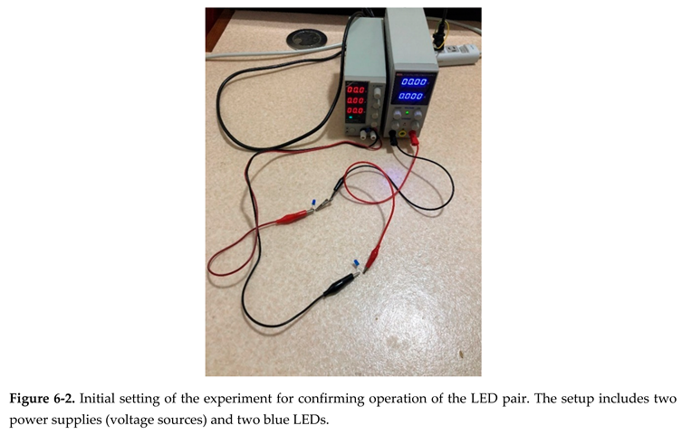
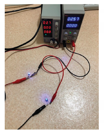
The results of the LED system are summarized in the following three figures: a schematic configuration of the circuit, a photograph of the initial experimental setup, and a photograph of the experimental result.
Figure 6.
Schematic of divergent current generation in the system with LED loads. As described in the main text, the divergent current drives the LEDs and the voltage sources die at steady-state.
Figure 6.
Schematic of divergent current generation in the system with LED loads. As described in the main text, the divergent current drives the LEDs and the voltage sources die at steady-state.
We now present the results of the paired motor system.
Figure 7.
Photograph of our tester, included for the reasons given in the Discussion.
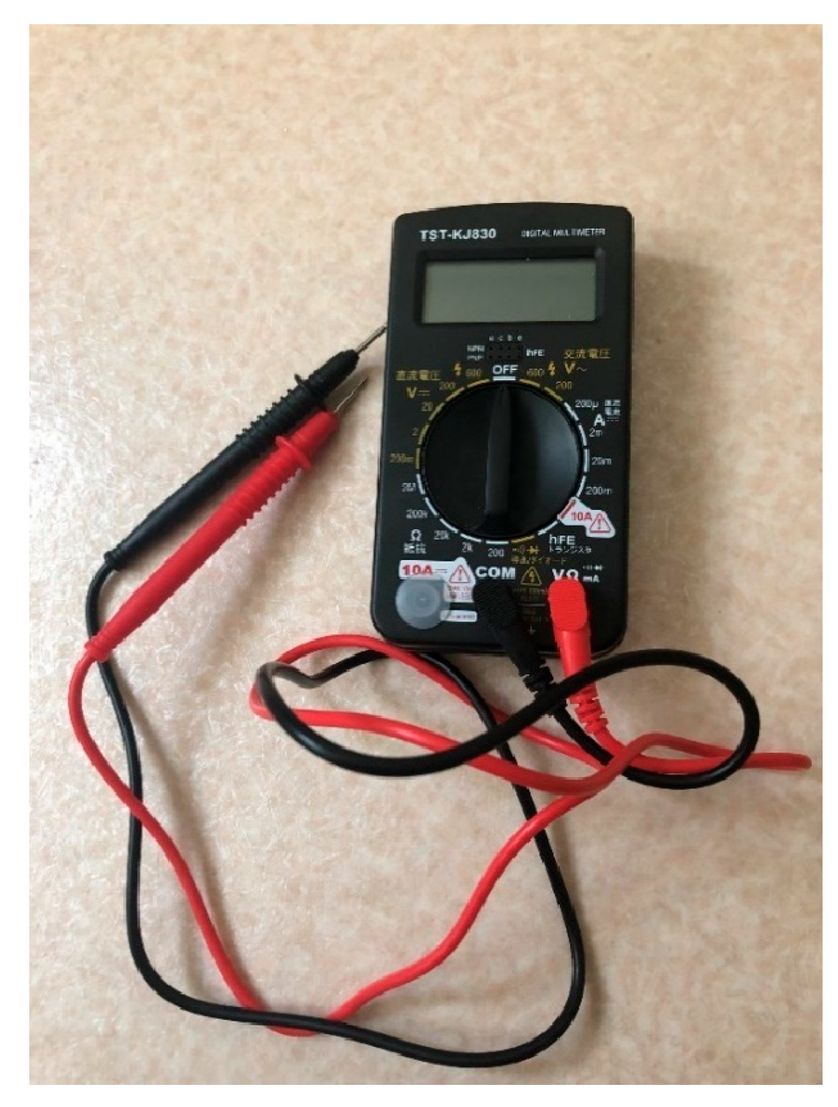
Figure 8.
Photograph of the paired DC motors (MABUCHI motor RE-280RA), marked with black dots to confirm whether the motors rotate during the experiment.
Figure 8.
Photograph of the paired DC motors (MABUCHI motor RE-280RA), marked with black dots to confirm whether the motors rotate during the experiment.
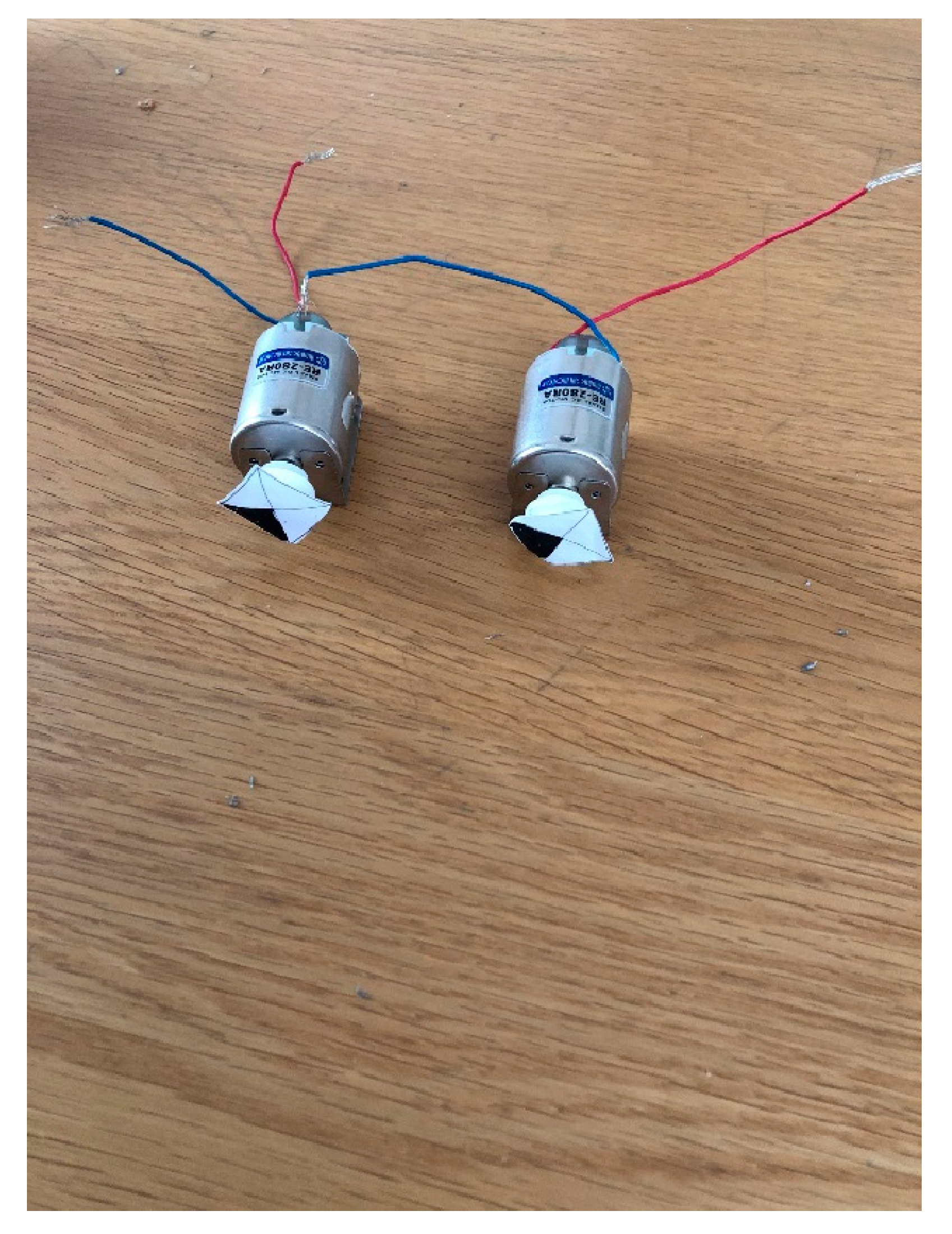
Table 1 lists the specifications of the employed DC motor, and Figure 7 and Figure 8 show a potable tester and the employed paired motors, respectively.
Figure 9 and Figure 10-1 present the three stages of the paired motor experiments: the circuit configurations, the preparations of the experiments, and the experimental results.
Figure 9.
Schematic of the circuit for measuring an emergent electric potential. The voltage of the voltage source is compared with that of the DC motor, which implies the emergent electric potential.
Figure 9.
Schematic of the circuit for measuring an emergent electric potential. The voltage of the voltage source is compared with that of the DC motor, which implies the emergent electric potential.
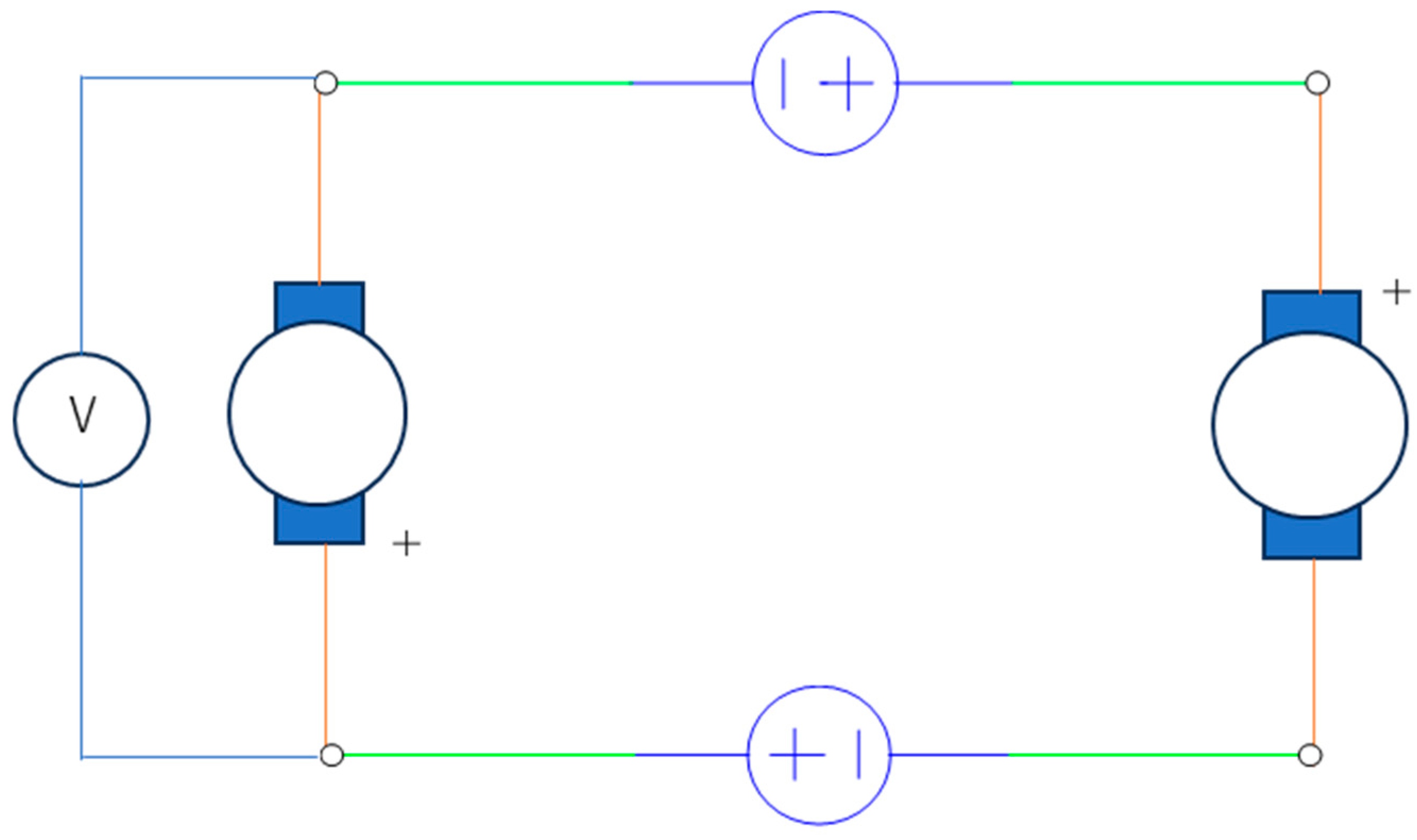
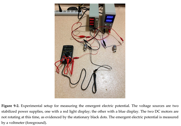
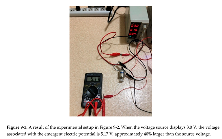
Figure 10.
Schematic of the experiment for harvesting the current I_E^'. As in Figure 5, a detour avoids interference between the induced macroscopic current I_a0 and the microscopic current I_E^'. As the mathematical form of the current I_E^' (0) is independent of the load R_0 and differs from Ohm’s law, the current flows even when the load R_0 is large. For the same reason, the load resistance R_0 generates no Joule heating. Note that |φ_(α,β) | will be described in the Discussion section.
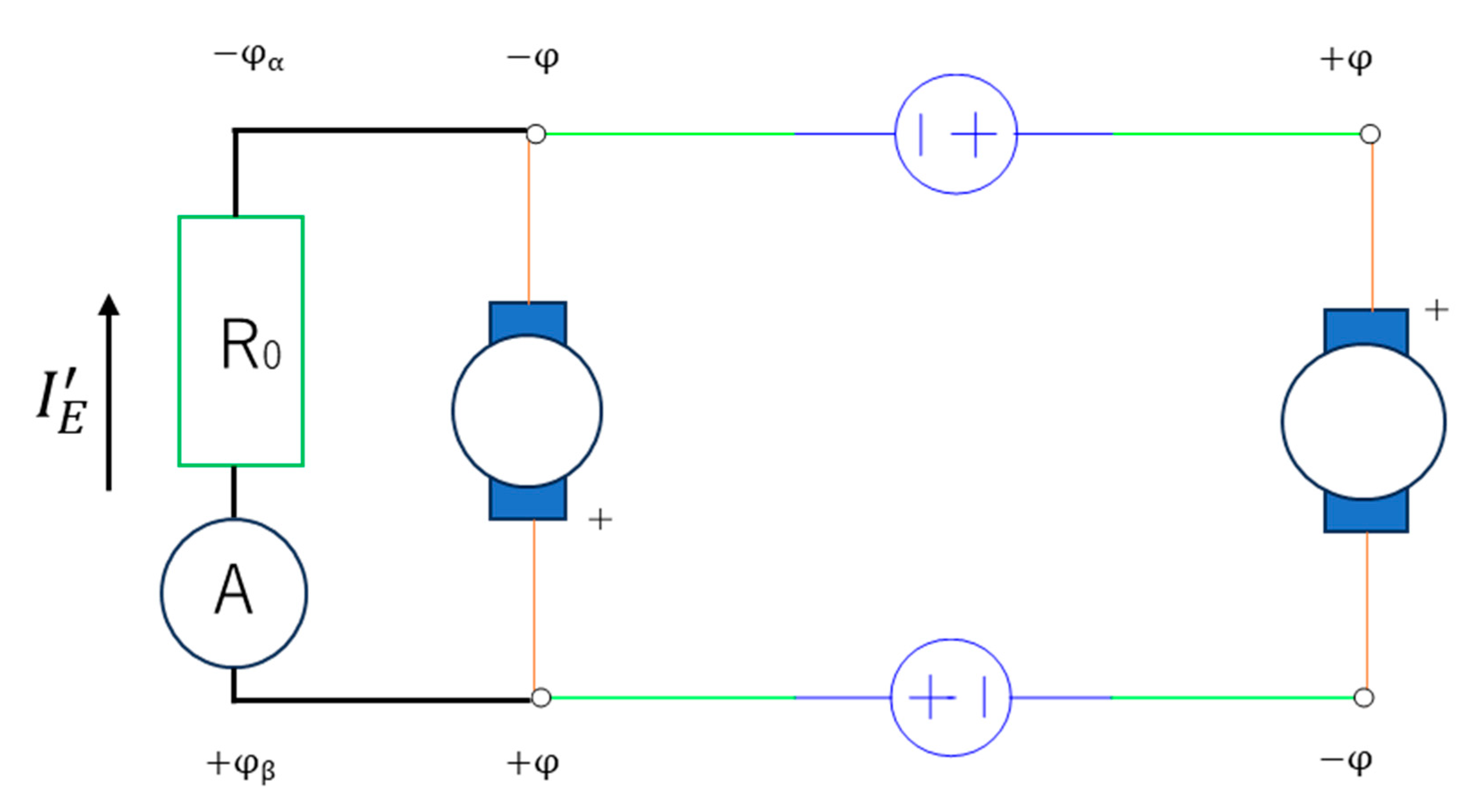
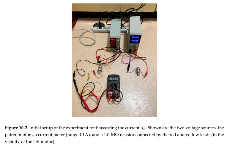
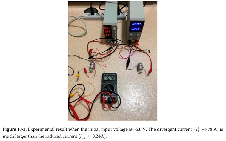
Figure 9-2. Experimental setup for measuring the
emergent electric potential. The voltage sources are two stabilized power
supplies, one with a red light display; the other with a blue display. The two
DC motors are not rotating at this time, as evidenced by the stationary black
dots. The emergent electric potential is measured by a voltmeter (foreground).
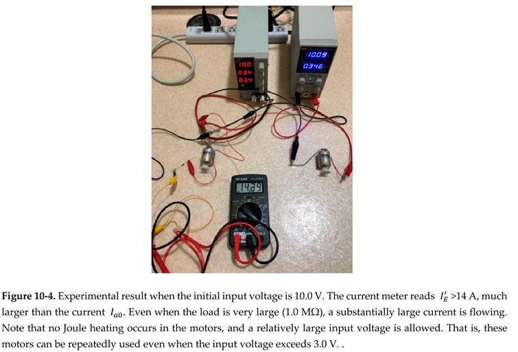
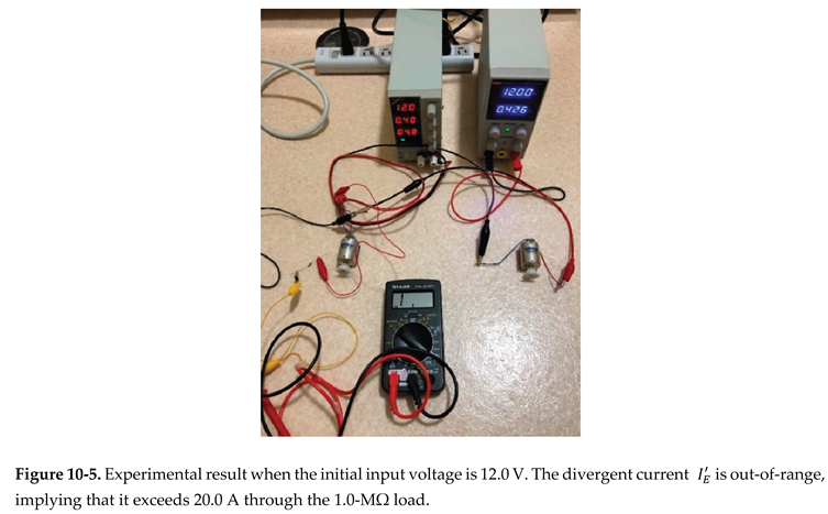
Table 2 compares the experimentally observed currents with the theoretical currents determined as:
where (E + Ec)/2 is the emergent electric potential (φ) with
As the emergent electric potential must not be significantly larger than the input electric potential (φe), we approximate
as a compromise. As shown, Table 2 confirms sufficient agreements between the experimental and theoretical values.
Table 3 lists the generated electric power (WR0) for different input voltages (2φe). Note that, in this table, (φ) in Eq. (71) is again defined by Eq. (82).The values of Table 3 are sufficiently large, which are almost equal to those of nuclear power stations. This implies that the values of Table 3 have provided significant technical merits.
For comfirmation, we validate Eq. (71); that is:
in the paired motor system. The electric power of the LED is obtained simply by replacing coefficient 0.45 [A/V2] with 0.04 [A/V2] as:
Assuming
And
we obtain
from which is calculated as:
On the other hand, the direct electric power W’LED is defined as simply
Then we get:
Thus
validating the expression of WLED. Considering that Eq. (83) (i.e., Eq. (71)) differs only in the coefficient (i.e., ), it is allowed to mention that the above result (91) also validates Eq. (71).
based on the previous results.
listed in Table 2.
Figure 11 shows the circuit configuration when another motor is employed as the detour. The detour motor operated only when its polarity was reversed from that of the paired motors. In this configuration, the additional motor exchanged energy with the left member of the motor pair. The exchanged energy is:
where E [V] are exchanged among [V], because the voltage (Ec) indirectly implies the loop current (Ia0) and if the motor M’ included this voltage (Ec), its current would also be the same loop current (Ia0). This case would claim that the current through the left menber of the paired motors becomes zero, considering the Kirchhoff’s current law. However, acutal experiments show that the left motor of the paired motors is still rotating. Accordingly, the voltage that makes the motor M’ work is [V].
4. Discussion
4.1. Why Can a Large Current Flow into the 1.0-MΩ Resistor?
A circuit containing a resistance (R) typically exhibits ohmic characteristics, meaning that its current depends on (R). However, in the present study,
which is independent of the resistance (R), meaning that the current flows through any resistor. The large current flow through the 1.0-MΩ resistor is explained not only by this phenomenon, but also by the absence of Joule heating under the imposed conditional inequalities.
4.2. Condition and Selection of the Paired Motor
To ensure that the paired DC motors satisfy the conditional inequalities (59) and (63), we recommend motors with relatively large inductances. However, inductors with excessive inductance should be avoided because they increase the internal resistance. Therefore, the paired DC motors must be carefully selected. This paper employs the previously discussed MABUCHI motor RE-280RA [23]. A trial experiment using coreless motors as the paired DC motors failed to display the phenomenon described here, possibly because coreless motors with relatively small inductances cannot satisfy the requisite conditions (59) or (63).
4.3. Why Is a Relatively Large Resistance Needed When Harvesting the Current?
To answer this question, we revisit Eq. (80):
, which implies that the voltage between taps α and β is [V]. When harvesting the current through a detour, the resistance (R0) should be sufficiently large to satisfy (see Figure 10-1)
where the left-side are electric potentials at tap α or β as a result of the flow of the current to the resistance (R0). Note that, even when the condition (93) is met, the emergent electric potential at each tap remains as , because the current must be constant, not increase. The reason is that, considering that Eq. (57) is formed and that no Joule heating implies the zero load of a motor, the zero-load motor implies that the rotational speed ( is the maximum . Thus, the absolute value of the voltage (E) under zero load is the maximum value.Thus the voltage of a motor is conserved. Thus, the electric potentials are not superposed at each tap. Assuming another stray condenser C0R parallel to both the sides of the paired motors, the stray condenser C0R of the left-side retains the electric potentials by charging energy, consuming the time constant: At the transient state, the sum of the current (ic) in the stray condenser C0R and the current in the resistance (R0) is equal to the constant current . First, the current flows along the stray condenser C0R but at the steady state this current flows through the resistance (R0). Although the resultant appear, the electric potentials do not increase as described.
If the condition (93) is satisfied, the current chooses the path along the detour instead of the path of the motor. This can be accepted by the fact that initially the motor inductor L generates magnetic field energy by the current and thus to reduce this energy at most, the current instead chooses the path of the resistance (R0). To put it precisely, the current chooses the shorted stray condenser C0R. Note that, if this condition is not satisfied and because a discharged current occurs from the inductor L of the left motor to the resistance (R0) due to a decrease in the absolute value of the voltgae (E), the current forms a loop current along R0-L and therefore this current decreases up to almost zero. To meet the condition (93), therefore, it is needed to employ a relatively large resistance as the detour.
When a current meter is placed along the detour, the electric potential at both the taps α and β should also satisfy the above condition. According to Figure 10-1, a relatively large load (R0) will enlarge the electric potential (φα). Moreover, our tester with a relatively large flow divider of a 10-A range is justified for boosting the electric potential (φβ). Note that, if a current meter that is to detect a small current is employed, the electric potential (φβ) becomes small.
Moreover, the phenomenon detected in the many experiments of this paper could not be detected by an autorange detector. Such a detector should be employed in a follow-up study, but an internal resistance that varies with the electrical signals might violate the above condition (93). Perhaps, there is a macroscopic current (iA) in autotange meter and thus this current (iA) might interefere with the microscopic current . Therefore, an autorange meter was not employed in our present experiments (Figure 7).
When another motor M’ is employed as a detour, energy exchanges between the inductors give rise to a constant current . As the additional motor has a very small internal resistance, it demonstrates the potential of supplying the current to a small resistance via the observed phenomenon.
4.4. Recap of the Key Concept
This paper describes a novel concept and a highly symmetric circuit for renewable energy generation. A circuit satisfying the requisite conditions generates a divergent current with no Joule heating. The divergent current drives both paired-LED and paired-DC-motor systems, generating large amounts of energy. The phenomenon is demonstrated both theoretically and experimentally, with good agreement between the theoretical and experimental results.
4.4. Significances of This Paper
Many countries are attempting to mitigate the pending energy crisis with solar cells, wind power, and biomass energy sources. However, natural energy produced by renewable energy sources inevitably fluctuate and destabilize the energy system. Stability can be restored only by introducing many storage batteries that increase the costs. More seriously, fossil fuel energies are major CO2 emitters, whereas nuclear power stations (which release no CO2) destroy the environment with radioactive materials and their wastes.
Our proposed methodology generates a large amount of energy using a highly symmetric circuit. The main contributions are listed below.
- 1)
- The net generated energy almost equals that of a nuclear power station, implying a sufficiently high energy density.
- 2)
- The system can be introduced at low cost (<10,000 yen).
- 3)
- The system generates no dangerous substances.
- 4)
- This system can provide the required amount of energy at the right time at the right place.
In summary, our simple-to-build system generates comparable energy to a nuclear power station.
5. Conclusion
This study proposes and verifies (theoretically and experimentally) a new circuit-based renewable-energy source. The system outputs a very high electric power and high energy density without natural fluctuations or dangerous substance production. That is, it harvests the required amount of energy at the proper time at the proper place.
Various motor types were experimentally trialed in the paired-motor system, but a more systematic experiment would consolidate the aforementioned conditions. Moreover, the capacitance of the stray capacitor is expected to slightly vary with humidity and atmospheric pressure. This expectation must be clarified in future work. Finally, the inapplicability of the autorange meter must be rationalized.
Additional Information
This study is unrelated to any competing interests such as funding, employment, or personal financial interests. Moreover, this study is unrelated to nonfinancial competing interests. This reasearch did not receive any specific grant from funding agencies in the public, commercial, or not-for- profit sectors.
Moreover, all original contributions and data associated with this study are included in the article. All data (raw) are presented as photographs in the Result section. Further inquiries can be directed to the corresponding author.
Acknowledgments
1) We thank Enago (www.enago.jp) for the English language reviews. 2) We appreciate the release of the preprints of the first and second versions: Ishiguri, S. Experimental Evidence of High Renewable Energy Employing a Symmetric Circuit with a Divergent Current Density. Preprints 2025, 2025042514. https://doi.org/10.20944/preprints202504.2514.v1. Ishiguri, S. Experimental Evidence of High Renewable Energy Employing a Symmetric Circuit with a Divergent Current Density. Preprints 2025, 2025042514. https://doi.org/10.20944/preprints202504.2514.v2
References
- S.R. Bull et al, Proceedings of the IEEE, 89(8), 1216 - 1226 (2001).
- Tyo et al, Entrep. Sustain., 7, 1514-1524 (2019).
- Dincer et al, Renew. Sustain. Energy Rev., 4, 157-175 (2000).
- M.R. Chehabeddine et al, Insights Reg. Dev., 4, 22-40 (2022).
- Adriaan van der Loos et al, Renew. Sustain. Energy Rev., 138, 110513 (2021). .
- Ellabban et al, Renew. Sustain. Energy Rev., 39, 748-764 (2014).
- R. Banos et al, Renew. Sustain. Energy Rev., 15 1753-1766 (2011).
- H. Obane et al, Renewable Energy, 160, 842-851 (2021).
- N.L. Panwar et al, Renew. Sustain. Energy Rev., 15 1513-1524 (2011).
- Sabishchenko et al, Energies, 13, 1776 (2020).
- M. Wierzbowski et al, Renew. Sustain. Energy Rev., 74, 51-70 (2017).
- C.-W. Wang et al, Energies, 13, 2629 (2020).
- T. Radavicius et al, Insights Reg. Dev., 3, 10-30 (2021).
- K. Akimoto et al, Energy and Climate Change, 2, 100057 (2021).
- K.O. Yoro et al, Renew. Sustain. Energy Rev., 150, 111506 (2021).
- J. P. Moriarty et al, Renew. Sustain. Energy Rev., 16, 244-252 (2012).
- J. A. Turner et al, Science 285, 687-689 (1999).
- S. Ishiguri. Preprints 2023, 2023061127.
- S. Ishiguri. Preprints 2024, 2024081690. 202.
- Einstein et al, Phys. Rev. 47, 777 (1935).
- S. Koide, Quantum Theory, p.3, Shokabo in Tokyo (1997).
- N. Matsui, Electrical Equipment, p.8, Morikita-Shuppan in Tokyo (2000).
- For the detailed specifications of the motor, visit the following: https://www.mabuchi-motor.co.jp/motorize/branch/motor/pdf/re_280ra.
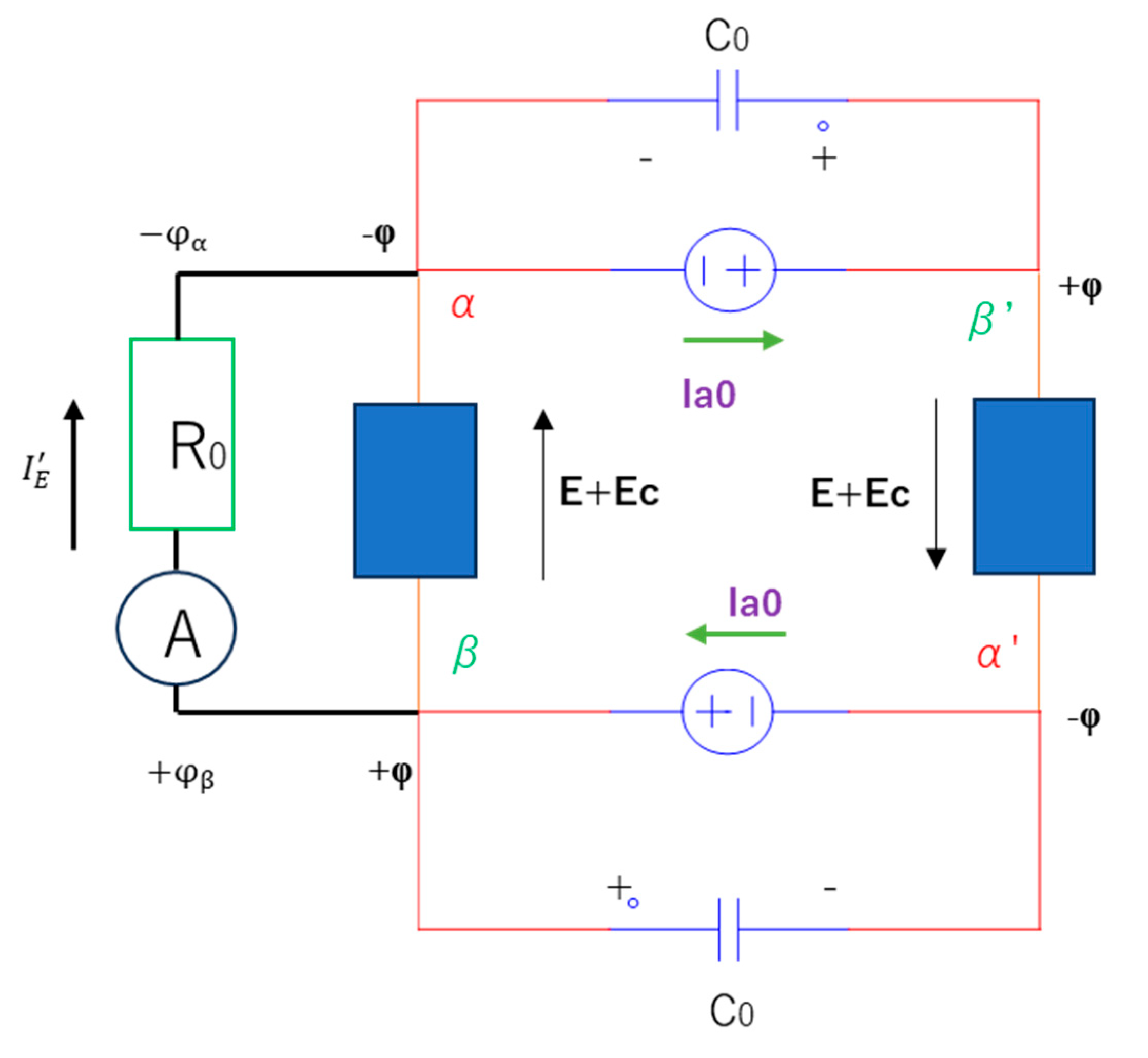
Figure 4.
Schematic showing the generation of induced currents Ia0 when the loads are DC motors. As (see Results section), the current Ia0 are induced by the inductances of the DC motors. As described for the paired stray capacitors, the paired-inductance L repetitively charge and discharges energy, generating a constant current Ia0 while the voltage sources V steadily decay.
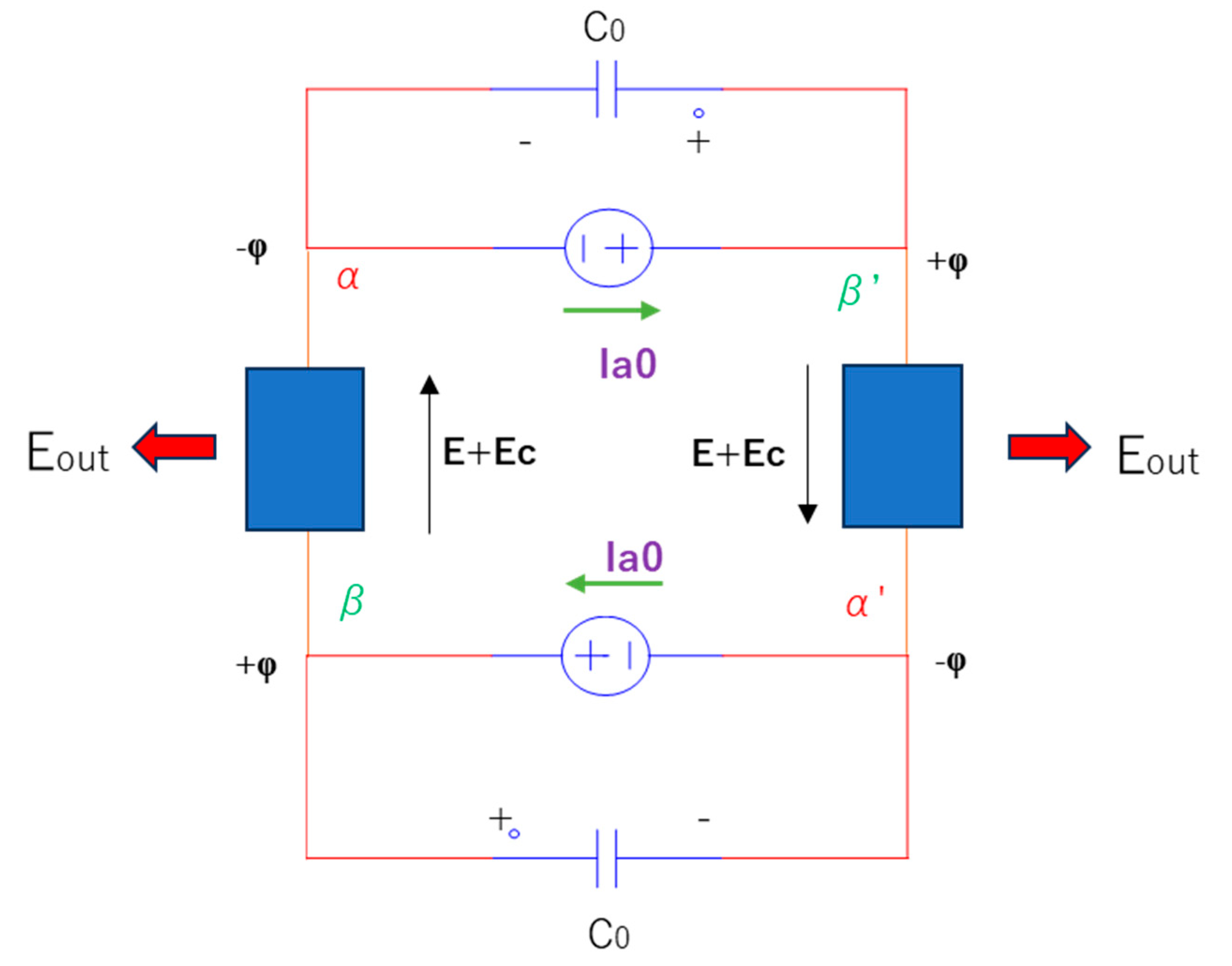
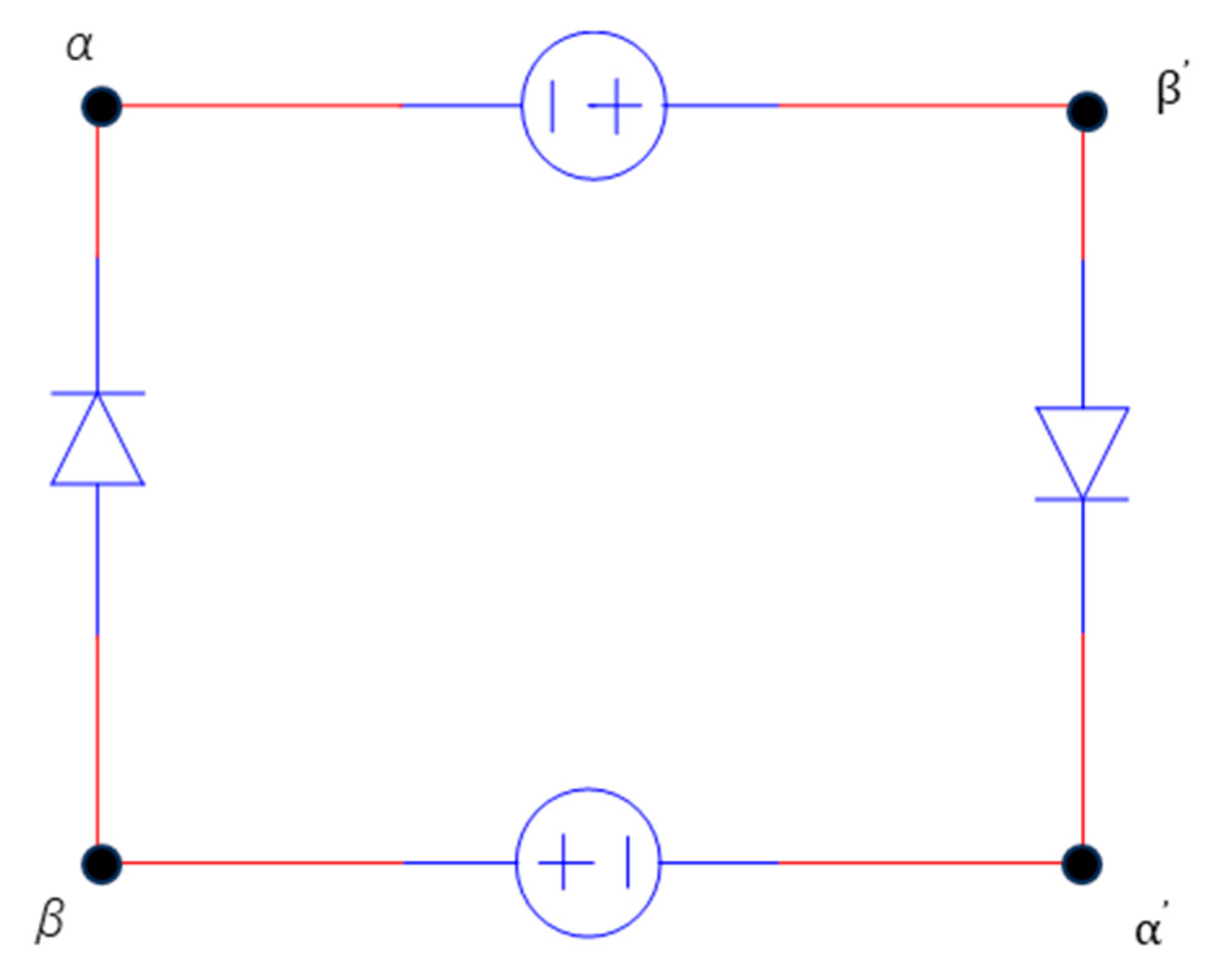
Figure 11.
Circuit configuration after inserting another motor as a detour. Note that the polarity (i.e. the direction) of each motor is important. That is, the polarity of M’ must be reversed from that of the paired motors and motor M’ rotates oppositely to the paired motors. If configured otherwise, M’ will not rotate. The photograph is omitted because motor M’ is not easily distinguishable; therefore, the photograph is noninformative.
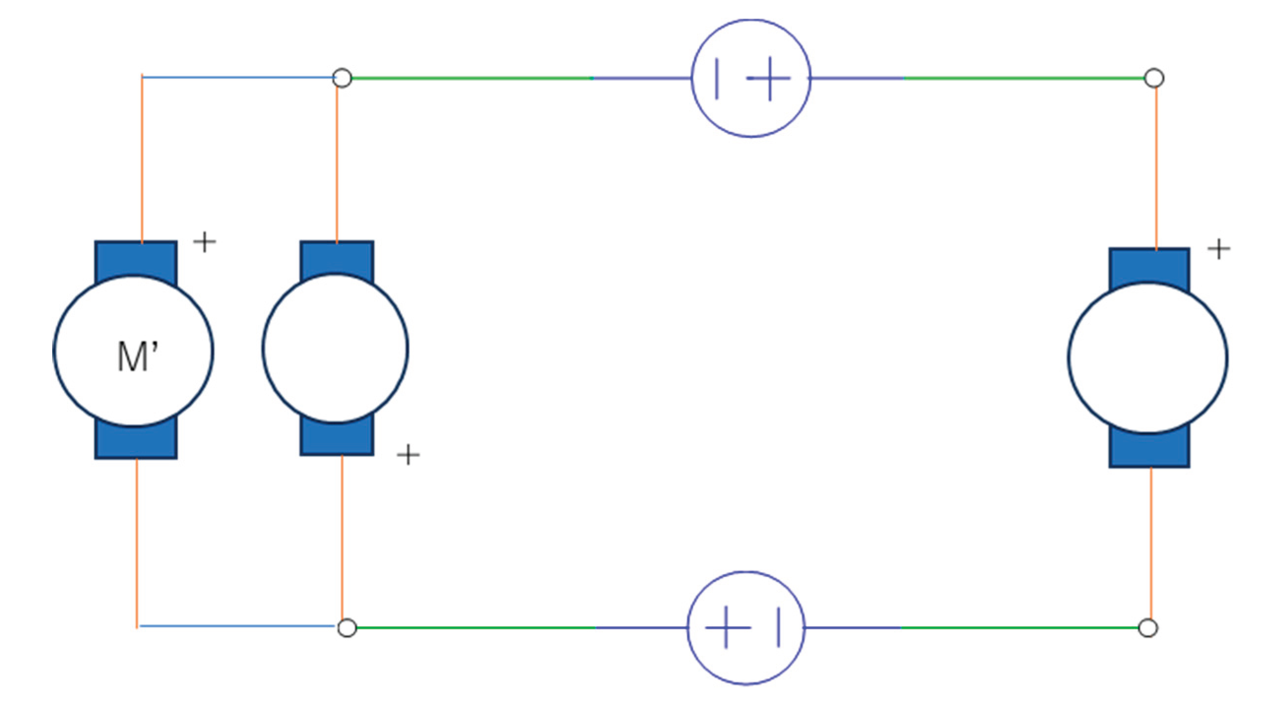

Table 1.
Motor specifications of the MABUCHI motor (RE-280RA).
| Normal voltage | |
| 3.0 V | |
| Normal Load |
1.47 |
| Speed at no Load | 8,700 r/min |
| Speed at normal Load | 5,800 r/min |
| Current at normal load | 650 mA |
| Shaft Diameter | 2.0 mm |
Table 2.
Comparisons of the experimental and theoretical currents
|
[V] |
for the theory |
for the experiment |
| 6.0 | 5.8 | 5.78 |
| 10.0 | 16.2 | 14.3 |
| 12.0 | 23 | More than 20 |
Table 3.
Output electric power WR0 evaluated for a 1.0-MΩ load resistance R0 and the theoretical divergent currents
Table 3.
Output electric power WR0 evaluated for a 1.0-MΩ load resistance R0 and the theoretical divergent currents
|
[V] |
WR0 [W] |
| 6.0 | |
| 10.0 | |
| 12.0 |
Disclaimer/Publisher’s Note: The statements, opinions and data contained in all publications are solely those of the individual author(s) and contributor(s) and not of MDPI and/or the editor(s). MDPI and/or the editor(s) disclaim responsibility for any injury to people or property resulting from any ideas, methods, instructions or products referred to in the content. |
© 2025 by the authors. Licensee MDPI, Basel, Switzerland. This article is an open access article distributed under the terms and conditions of the Creative Commons Attribution (CC BY) license (http://creativecommons.org/licenses/by/4.0/).
Copyright: This open access article is published under a Creative Commons CC BY 4.0 license, which permit the free download, distribution, and reuse, provided that the author and preprint are cited in any reuse.


