
Submitted:
29 April 2025
Posted:
07 May 2025
You are already at the latest version
Abstract
Integrated adaptive algorithms (IAA) are widely used in control systems. Some authors use integrally proportional algorithms, which are obtained in heuristically considered features of the system under consideration. Most IA was got based on of the second Lyapunov method. Modifications of numerical procedures are used as algorithms for tuning parameters of the control law. In this paper, we substantiate some well‐known algorithms and procedures, considering the requirements for an adaptive identification system. Requirements are formed as functional constraints and are considering during synthesis. A representation of the adaptive algorithm is obtained as a system in the state space. Classes of potential algorithms (PA) are considered. PA has a general form and is required adaptation at the implementation stage. PA variants are presented. The limitation of trajectories in an adaptive system and their exponential stability are studied. Simulation results are got.
Keywords:
adaptive algorithm
; functional constraint
; adaptive system
; exponential stability
; Lyapunov function
1. Introduction
The integrated adaptive algorithm (IAA) is widely used in control systems:
where is vector of tuning parameters; is an error in estimating system output; is vector of observed variables (input, control); is positive definite gain matrix; is the matrix of the loss function (optimisation criteria).
Equation (1) describes the IAA class, which determined by minimising the quadratic loss function, consider heuristic assumptions, or ensuring the stability of the identification system (see, for example, [1,2,3,4,5,6,7,8,9,10]).
In [6], the system is considered
where are vectors of state and control; is a continuous vector function; and are continuous matrix functions, is an undefined function; is an unknown parameter vector. A preliminary estimate is known for .
A robust adaptive algorithm (AA) [6] is proposed:
where is estimation of the vector, is control, , is a matrix that determines the quality of control.
The algorithm (3) implementation under uncertainty is difficult, since the current evaluation of the adaptation quality is not considered. Modification (3) and its simplifications are proposed in [6].
In [10], IAA (1) and its proportional -modification were considered [11]
where guarantees damping of the tuning process.
A generalization of the -modification, if the condition of constant excitation is not fulfilled, is given in [12]. In [12], the design of AA is based on the requirements for the derivative of Lyapunov function (LF).
An adaptive law for the first-order system is proposed in the form
where , is error in predicting system output, is generalised system input, . AA is introduced intuitively without synthesis formalization method.
Projection variants of IAA are proposed in [13]. Modifications of IAA are considered in [15,16,17,18]. A normalized version of the algorithm (1) (projection algorithm) is proposed in [16]
where . Various projection AA is considered in [19].
Regardless of [12], in [20], an analytical method is proposed for the synthesis of adaptive algorithms, considering functional limitations.
Remark 1. Sometimes, signalling adaptation (SA) [21] algorithms are used. As shown in [20], the SA use in adaptive identification systems is not always effective.
The analysis shows that the IAA is obtained based on the least squares method and its modifications, and the LF, are mainly used. Gradient algorithms based on numerical optimisation methods are often implemented. The AA parameters are selected to ensure the stability of the adaptive process.
In this paper, we generalise the approach proposed in [20] for the formalised synthesis of AA. The properties of the adaptive identification system (AIS) are investigated using the example of a decentralised system.
2. Problem Statement
Consider AIS
where is the state vector, is a matrix with constant elements, , , is system output.
Set of experimental data
The model for evaluating elements
where is the Hurwitz matrix, is the model state vector, and are tuning matrices.
Problem: find the tuning laws of the matrices G1 and K2 such that:
3. The Constant Excitation Condition
Consider the requirements for . The estimation of system parameters (1) depends on the -system identifiability. This property is guaranteed if the condition of constant excitation (CE) is satisfied for .
Let satisfy the condition CE
where , . If does not have the CE property, then we will write or .
Remark 2. If a nonlinear System is considered, then condition (8) is transformed [22].
4. AA Synthesis Based on LF
The error equation for the system (1), (7):
where ; are parametric residuals.
Let a functional constraint be imposed on the system (9), where is a continuously differentiable function reflecting the tuning process quality. The task is reduced to meeting the target condition .
Introduce LF
where is symmetric positive definite matrix, is the trace of the matrix, are diagonal matrices.
The derivative:
where , is symmetric positive definite matrix. From we obtain AA
So, the IAA synthesized from the stability condition of the system (9). AIS is stable in the space . This is a classic AA synthesis scheme.
Remark 3. In [18], a quadratic condition is imposed on to develop a control algorithm. Functional restrictions (FR) for obtaining AA are not considered.
5. FR and AA Structure
Consider LF and apply the approach [20]. Let FR imposes on the AIS
where is a quality function of processes in the adaptive system.
Describe the approach to AA synthesis using the example of the matrix identification for the -system. Let . Consider examples of functions .
1. , where . Let . Then:
From condition , we obtain
Let . We get the representation for equation (15) in the state space
So, if FR is imposed on AIS, then AA is described by the system . In this form, to apply of the system (16) is difficult. Therefore, the system structural modification is necessary (16).
Remark 4. There are various modifications to the -system that depend on FR.
2. и . Then we get the -algorithm:
where , is the Euclidean norm of the vector .
Modifications of the -algorithm:
(a) integral -algorithm
where , ;
(b) -algorithm as a delayed system (modification (17)):
where , is time lag;
(c)
Remark 5. The AA (17) implementation and its modifications is depended on the identified system and the properties of the set . At the beginning of the adaptation, apply variant (17). If the initial conditions can be chosen successfully, then apply algorithms (18)–(20).
3. , where , is the diagonal matrix of the vector elements. corresponds to the -algorithm
Remark 5 is valid for (21). Modifications and simplifications of the G2 algorithm are possible. As a special case, algorithm (5) follows from (20).
Remark 6. FR can have a different form. Above, we have considered only some examples of restrictions for adaptive identification of matrix . The described approach is valid for the vector identification. If in variant (2b) , then we get of the algorithm (18) analog from (20), a special case of which is equation (6).
6. AIS Properties
We will evaluate the limitations of AIS trajectories using algorithms (19) and
Theorem 1. Let: 1) is the Hurwitz matrix; 2) Lyapunov functions and assume an infinitesimal upper limit, where are diagonal matrices with positive diagonal elements; 3) , ; 4) 4) exists such that the condition
is performed at sufficiently large in some neighbourhood of zero. Then the trajectories of the system (9), (19), (22) are bounded on some set of initial conditions if
where , , is the minimum eigenvalue of the matrix.
The proof of Theorem 1 is presented in Appendix A.
Theorem 1 confirms the limited trajectories in the system (9), (19), (22) and the possibility of local identifiability of model parameters. These statements are valid for some set of initial conditions, since AIS is a system with the delay.
Consider the system (9), (15). To simplify the results, we assume that the vector of the model (7) is precisely tuned (i.e., ), and:
Present the algorithm (15) in the form (see Appendix B)
In (26), the argument is omitted, and is used to emphasise the delay.
Consider FL and the Lyapunov
depending on initial conditions for .
Theorem 2. Let the theorem 1 conditions be fulfilled, where the functional (26) is used instead of , and 1) exists such that the condition
is performed at sufficiently large in some neighbourhood of zero; 2) the system of inequalities
is fair, where are numbers depending on the parameters of the adaptive system; 3) the upper solution for the Lyapunov vector function satisfies the comparison system if , where are initial conditions for elements of corresponding vectors, . Then the adaptive system (25), (19), (26) is exponentially stable with the estimate
If , , are the maximum eigenvalue of the matrix, .
The proof of Theorem 1 is presented in Appendix C.
Theorem 2 proofs the exponential stability of the adaptive system (AS) with algorithm (26). We apply the Lyapunov functional (27) to prove this property.
Remark 7. Consider the tuning algorithm (26) does not change the statement of Theorem 2. In this case, the system of inequalities is valid (28).
So, we have proved the applications of AA as a dynamic system. These algorithms improve the quality of tuning process for model parameters.
Consider AIS (9), (21) with the algorithm
where is the diagonal matrix.
Theorem 3. Let conditions 1-3 of Theorems 1 be fulfilled and 1) exists such that the condition is performed at sufficiently large in some neighbourhood of zero; 2) the system of inequalities
is fair, where , , are positive numbers depending on the parameters of the adaptive system; 3) the upper solution for the Lyapunov vector function satisfies the comparison system if , where are initial conditions for elements of correspond vectors, . Then the adaptive system (9), (21), (29) is exponentially stable with the estimate:
if , and .
Remark 8. Properties of IAA obtained without restrictions depend on the CE condition fulfilment.
7. Simulation Results
Consider the system
where , are state vector and output of the subsystem ; is input (control); is saturation function; is the sign function; is output of the subsystem , , , , , , , , . inputs were sinusoidal.
Models for the system (31)
where , , , are tuning parameters.
Adaptive algorithms
where .
Results are shown in Figure 1, Figure 2 and Figure 3. s 1 reflects the adequacy of the models (33), (34).
Figure 1.
Adequacy of models (33) and (34): 1 is model (33), 2 is model (34).
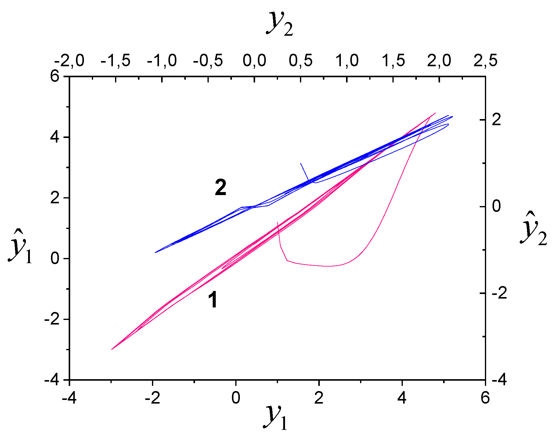
Figure 2.
Tuning parameters of model (33).
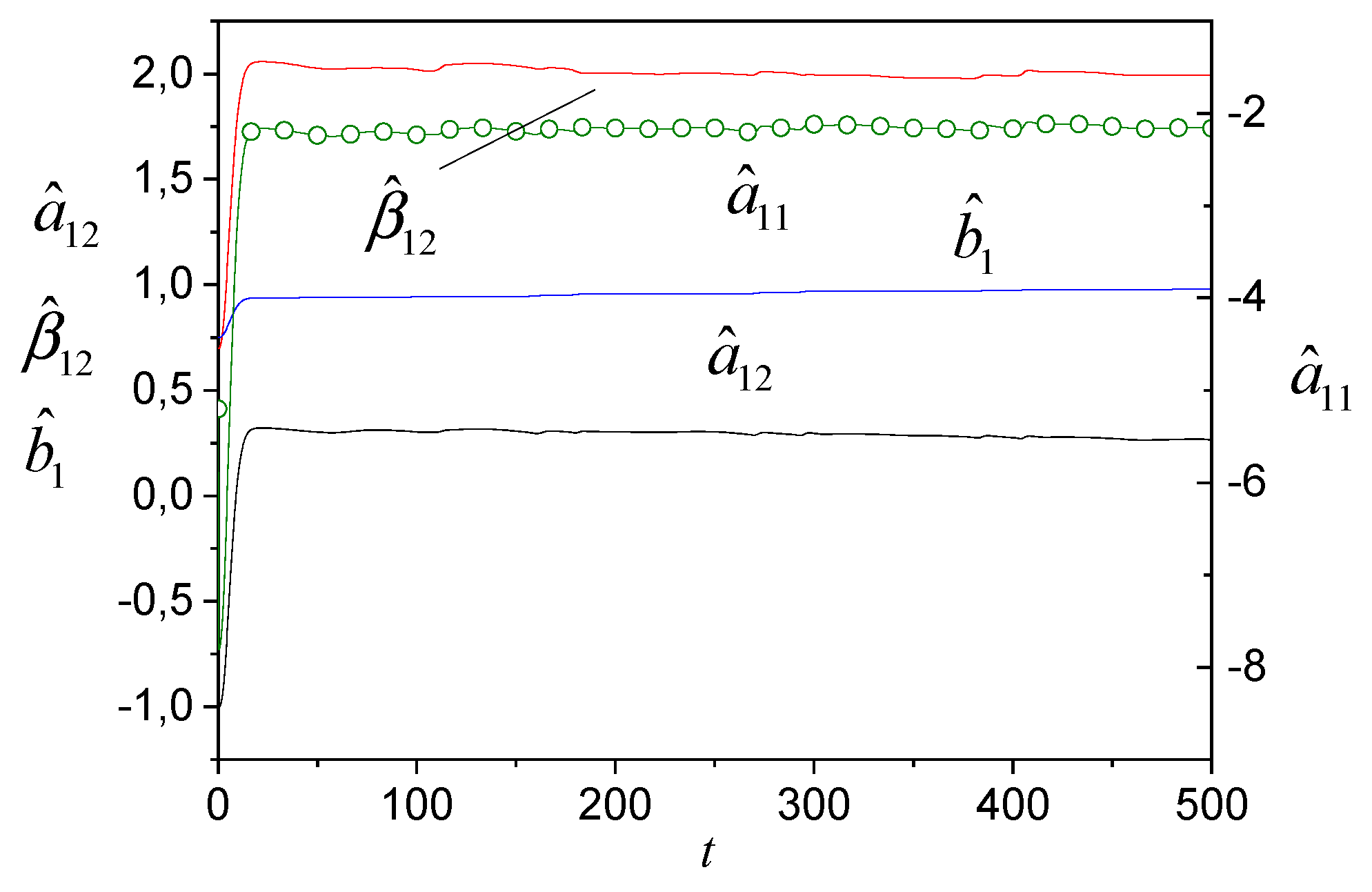
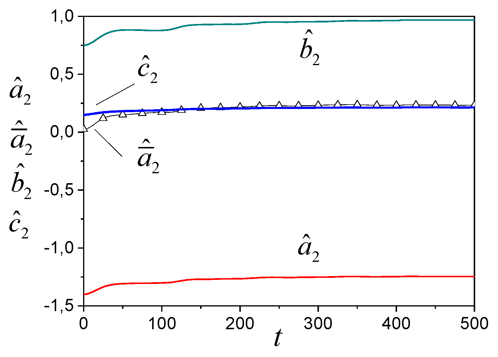
Figure 3.
Tuning parameters of model (34).
Simulation results confirm the proposed AA performance. (35) and (36). Tuning process can be linear or nonlinear. Efficiency is determined by properties of the adaptive system and the parameters of signals.
In Figure 4, Figure 5 and Figure 6, we present identification results of the system (31) with algorithms (35), (36), where algorithms for tuning and in (35) have the form
To ensure the system (31) S-synchroniability, we changed parameters and . Tuning parameters for models (33) and (34) are shown in Figure 4 and Figure 5. The adequacy of the models is reflected in Figure 6.
Figure 4.
Tuning parameters of model (33): 1– , 2 – , 3 – , 4 – , 5 – .
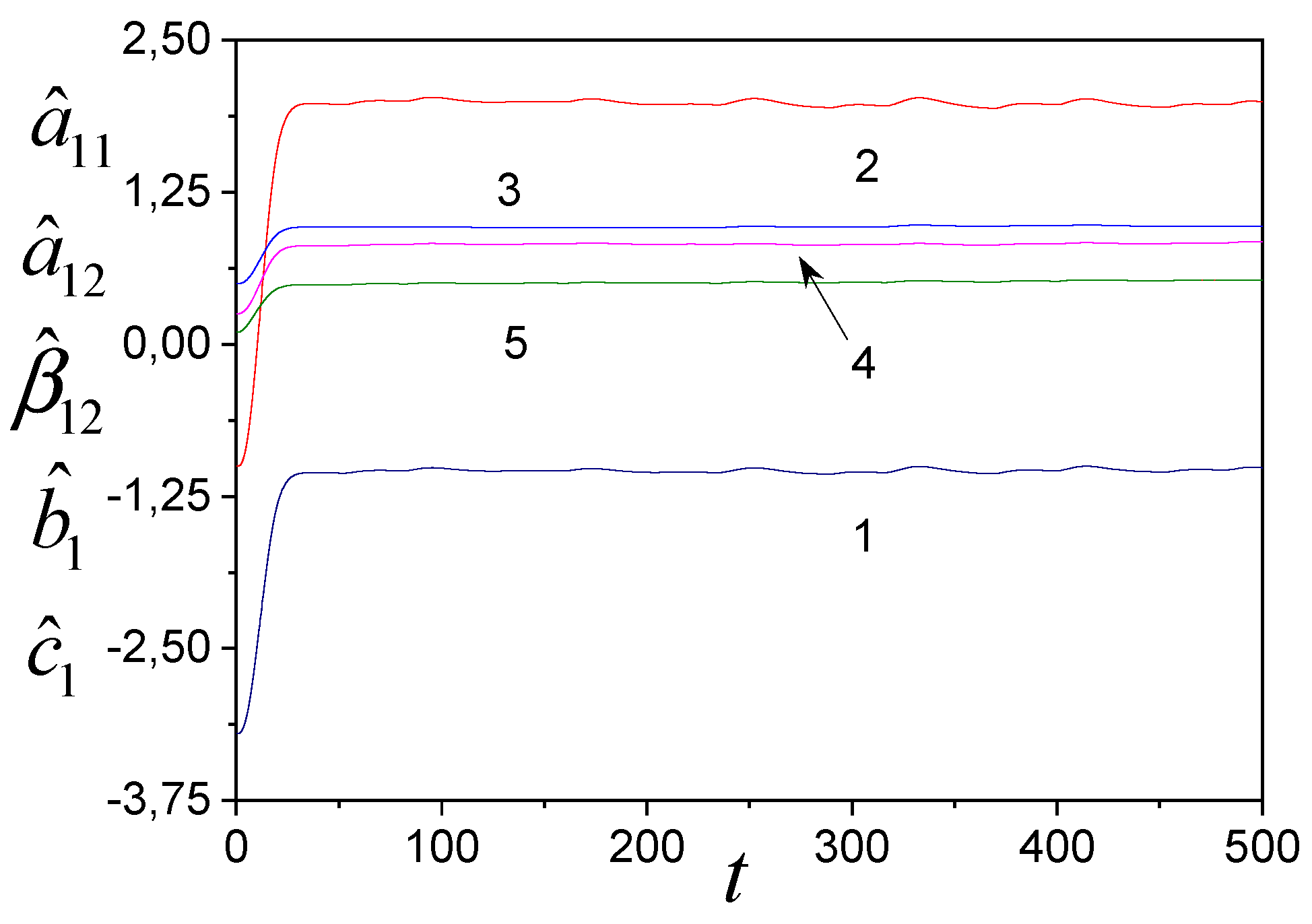
Figure 5.
Tuning parameters of model (34): 1 is , 2 is , 3 is , 4 is .
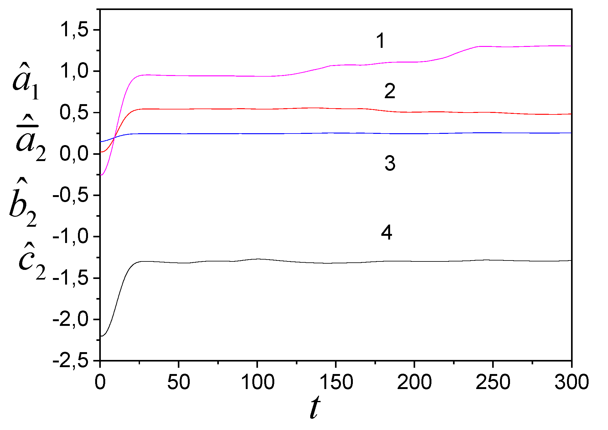
Figure 6.
Adequacy of models (33) and (34).
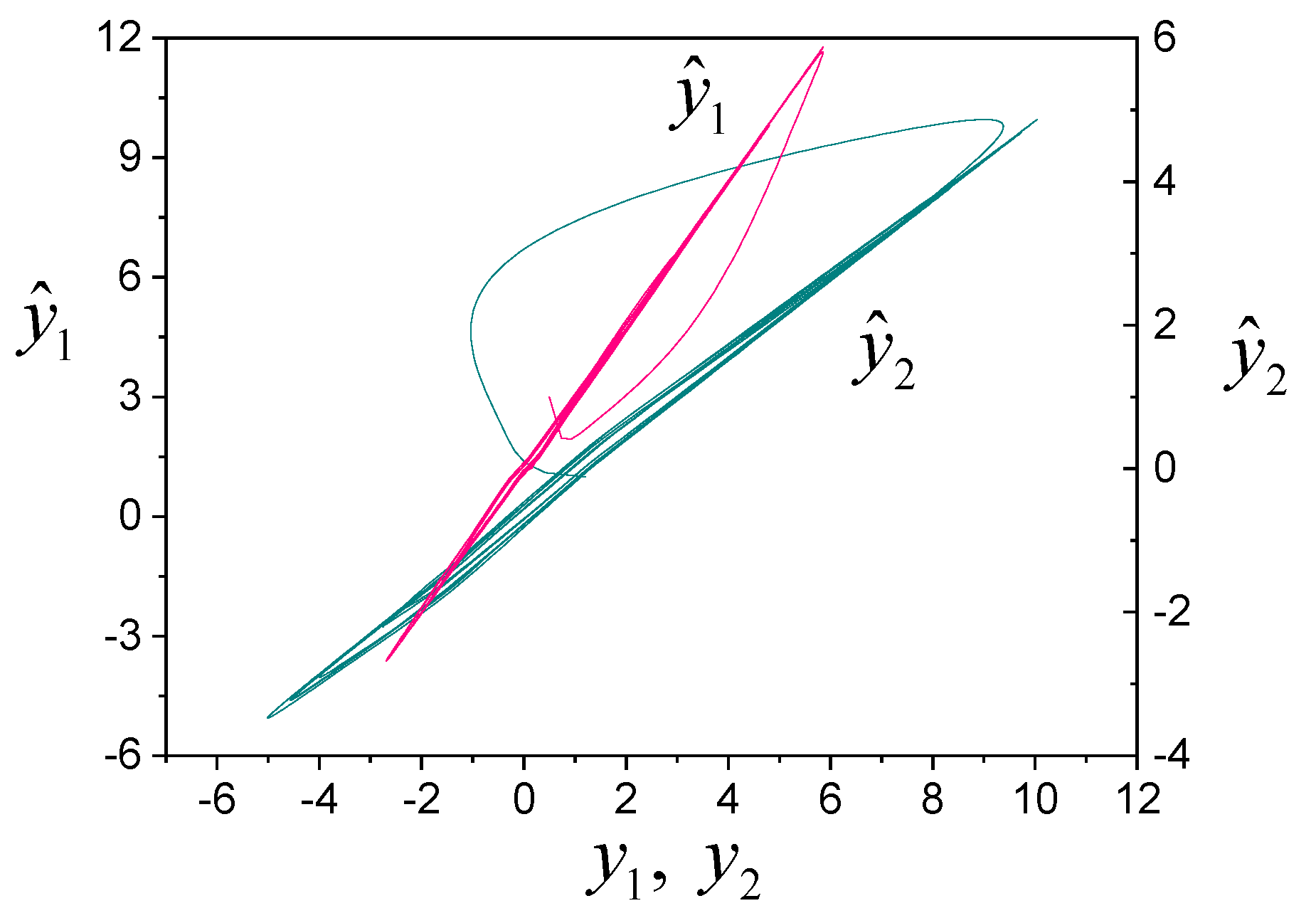
We see that the outputs of subsystems affect adaptation processes.
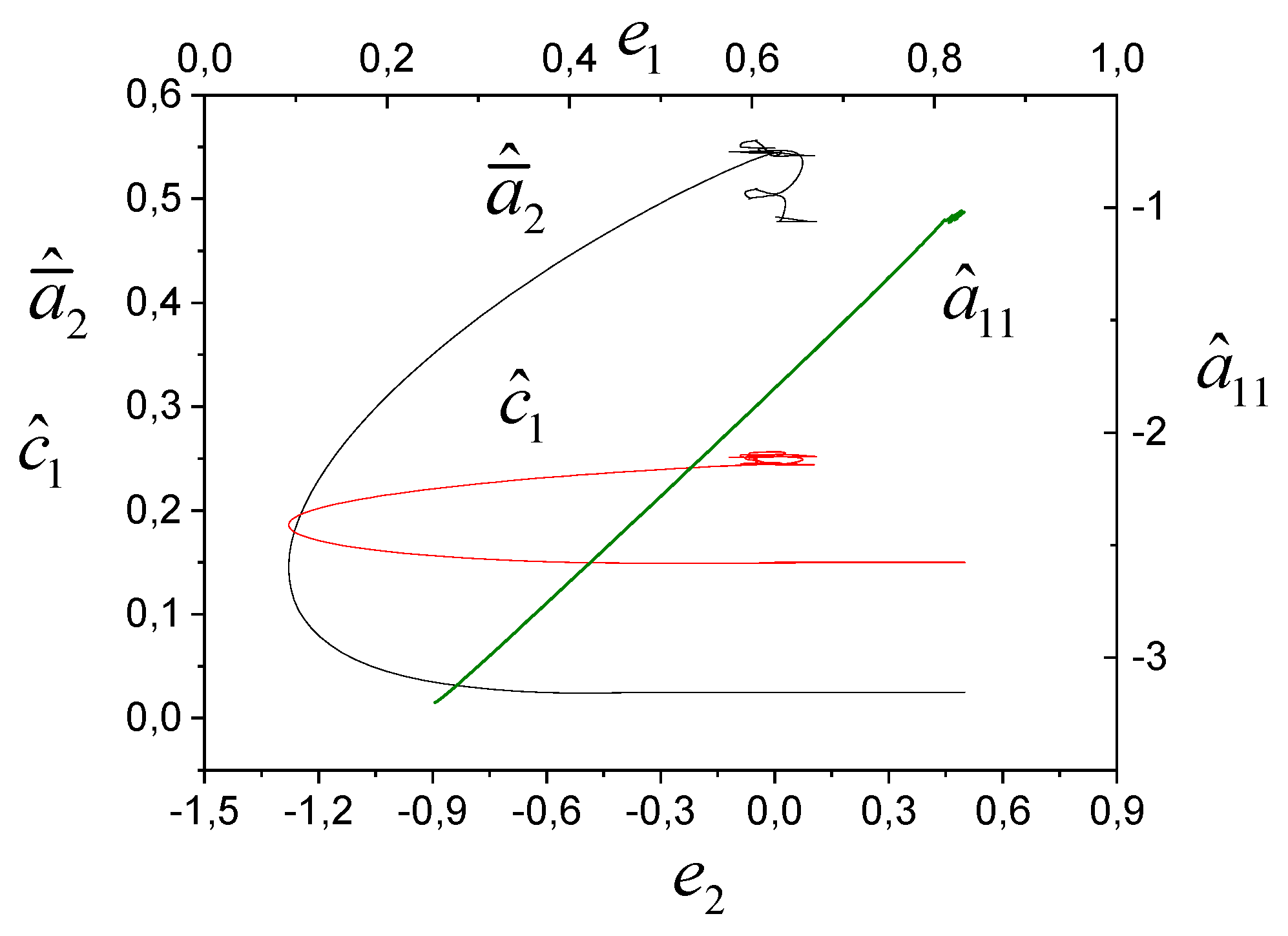
Figure 7 shows phase portraits in AIS in spaces и , . We see that adaptation processes for are nonlinear, and they are almost linear for the system.
Figure 7.
Phase portraits of AIS in spaces , and .
So, the simulation results confirm the proposed algorithms.
8. Conclusion
The approach to the synthesis of adaptive algorithms based on requirements for the adaptation process is proposed. These requirements are presented as functional constraints (FR). It is shown that, for the considered class of FR, the adaptive algorithm is described by the system in the state space. Special cases of FR are considered and the corresponding AA are obtained. For one class of adaptive algorithms, a representation is presented as the dynamic system with an aftereffect. Properties of adaptive systems of identification are studied, and the limited of trajectories and exponential stability are proved. Simulation results confirm the efficiency of adaptive algorithms.
Appendix A
Proof of Theorem 1. Consider FL
For , we get
or
where , , is a symmetric positive matrix.
Let , . As
where , are maximum eigenvalues of matrices , , then
where .
is
The component depending on :
Then
and
where . Condition (23) is valid for . Therefore,
As
then (A6)
where . After simple transformations, we get
Apply the inequality
and get
where .
The component depending on :
Get
As
then
or
So
where .
Let , and . Then, considering (A7) and (A9), we get
From (A10) we obtain that trajectory of the system (9), (19), (22) are limited if the condition
is satisfied on a certain set of initial conditions. □
Appendix B
Obtain to algorithm (25). Present the algorithm (15) as:
Let , where , is the discreteness step. Then (B1) present as:
where . The algorithm (B2) is rewritten as:
where , .
Appendix C
Proof of Theorem 2. Following the proof of Theorem 1, we obtain for :
Let , , , and , where . As then
where , .
Consider . We get for :
Transform (C3)
Let . Then (C4):
Let
Then
where , . As , then we get by the mean integral theorem (or the Newton-Leibniz formula)
Let . Then
So, the system of inequalities is valid for the system (25), (26)
The upper solution of the system (C8) satisfies the vector system if , where are initial conditions for elements of vectors , . The adaptive system is exponentially stable with the estimate:
if , . □
Appendix D
Proof of Theorem 3. Consider AS (9), (21), (29). Apply FL from theorem 1., We obtain (see (A3)) for :
where , are maximum eigenvalues of matrices , , .
Present for
Let
where , . Then (D2)
Let , then
where . As
then
where .
So, for , we obtain
Estimation of exponential stability for the system
where is a comparison system for (D5), if , where are the initial conditions for elements of corresponding vectors.
The estimate (D6) is valid if and . □
References
- Narendra K. S., Annaswamy A. M. Robust adaptive control in the presence of bounded disturbances. IEЕЕ Transactions on automatic control, 1986; 31(4);306-315.
- Nikolić T., Nikolić G., Petrović B. Adaptive controller based on LMS algorithm for grid-connected and islanding inverters. Proceedings of the 8th Small Systems Simulation Symposium 2020, Niš, Serbia, 12th-14th February 2020, 2020;107-110.
- Polston J. D., Hoagg J. B. Decentralized adaptive disturbance rejection for relative-degree-one local subsystems. 2014 American Control Conference (ACC) June 4-6, 2014. Portland, Oregon, USA. 2014; 1316-1321. [CrossRef]
- Lozano R., Brogliato B. Adaptive control of robot manipulators with flexible joints. IEEE Transactions on automatic control, 1992; 37(2);171-181. [CrossRef]
- Landau I.D., Lozano R., M’Saad M., Karimi A. Adaptive control algorithms, analysis and applications. Second edition. Springer: London Dordrecht Heidelberg New York, 2011.
- Duan G. High-order fully actuated system approaches: Part V. Robust adaptive control. International journal of systems science, 2021;52(10); 2129–2143. [CrossRef]
- Landau Y. D. Adaptive Control: The Model reference approach. Dekker, 1979.
- Kaufman H., Barkana I., Sobel K. Direct adaptive control algorithms: theory and applications. Second edition. Springer, 1998.
- Hua C., Ning P., Li K. Adaptive prescribed-time control for a class of uncertain nonlinear systems. IEEE transactions on automatic control, 2022;67(11); 6159-6166.
- Weise C., Kaufmann T., Reger J. Model reference adaptive control with proportional integral adaptation law. 2024 European Control Conference (ECC) June 25-28, 2024. Stockholm, Sweden, 2024; 486-492.
- Ioannou P., Kokotovic P., Instability analysis and improvement of robustness of adaptive control, Automatica, 1984;20(5); 583–594. [CrossRef]
- Narendra K., Annaswamy A. A new adaptive law for robust adaptation without persistent excitation, IEEE Transactions on automatic control, 1987;32(2);134–145. [CrossRef]
- Lavretsky E., Gibson T. E., Annaswamy A. M. Projection operator in adaptive systems. 2012, arXiv:1112.4232. [CrossRef]
- Chen Z., Yang T. Y., Xiao Y., Pan X., Yang W. Model reference adaptive hierarchical control framework for shake table tests. Earthquake Engng Struct Dyn. 2025;5(4);346–362. [CrossRef]
- Brahmi B., Ghommam J., Saad M. Adaptive observer-based backstepping-super twisting control for robust trajectory tracking in robot manipulators. TechRxiv. September 18, 2024. [CrossRef]
- Narendra K. S., Han Z. Adaptive control using collective information obtained from multiple models. Proceedings of the 18th World Congress the International Federation of Automatic Control Milano (Italy) August 28 - September 2, 2011; 362-367.
- Narendra K. S., Tian Z. Adaptive identification and control of linear periodic systems. Proceedings of the 45th IEEE Conference on Decision & Control Manchester Grand Hyatt Hotel San Diego, CA, USA, December 13-15, 2006; 465-470.
- Krsfić M., Kanellakopoulos I., Kokotović P. Nonlinear and adaptive control design. John Wiley & Sons, Inc, 1995.
- Hovakimyan N., Cao C. L1 adaptive control theory: guaranteed robustness with fast adaptation. SIAM, 2010.
- Karabutov N. Identification of decentralized control systems. Preprints.org (www.preprints.org), 2024. [CrossRef]
- Podval’ny S.L., Vasil’ev E.M. Multi-level signal adaptation in non-stationary control systems. Voronezh state technical university bulletin, 2022;18(5);38-47.
- Karabutov N. N. Structural Identifiability evaluation of system with nonsymmetric nonlinearities. Mekhatronika, Avtomatizatsiya, Upravlenie, 2024;25(2);55-64. [CrossRef]
Disclaimer/Publisher’s Note: The statements, opinions and data contained in all publications are solely those of the individual author(s) and contributor(s) and not of MDPI and/or the editor(s). MDPI and/or the editor(s) disclaim responsibility for any injury to people or property resulting from any ideas, methods, instructions or products referred to in the content. |
© 2025 by the authors. Licensee MDPI, Basel, Switzerland. This article is an open access article distributed under the terms and conditions of the Creative Commons Attribution (CC BY) license (http://creativecommons.org/licenses/by/4.0/).
Copyright: This open access article is published under a Creative Commons CC BY 4.0 license, which permit the free download, distribution, and reuse, provided that the author and preprint are cited in any reuse.


