
Submitted:
21 April 2025
Posted:
22 April 2025
You are already at the latest version
Abstract
Particle accelerator laboratories, which enable world-class research across many scientific fields, depend on the magnets used to manipulate their particle beams for successful operation. The community employs various techniques, typically based on Hall probes and induction sensors/coils, to verify the performance of accelerator magnets. Conventional Hall probe systems cannot be deployed, or require significant modification, when the transverse access around a magnet is restricted; meanwhile, moving wire/coil systems tend to provide information only on the B field’s integral. This research builds upon a vibrating wire setup first commissioned to locate the magnetic center of quadrupole magnets. Scans up to the n=200 wire harmonic (∼10 kHz drive frequency) were measured to reconstruct the B field across a vibrating wire strung through a test magnet. New software was developed to systematically process the many wire harmonics needed for a detailed field reconstruction. This research investigated the speed and precision of the measurement, identifying limitations due to both instrumentation and nonlinear wire behaviour at very high harmonic. The vibrating wire data agreed with a reference Hall probe scan on the order of 6%; roughly 0.7% RMS error persisted after calibrating the vibrating wire data to the reference scan via scaling factor.
Keywords:
magnetic measurement
; vibrating wire
; Hall probe
; frequency response
; nonlinear wire dynamics
1. Introduction
From multipole magnets, such as quadrupoles, to insertion devices, such as undulators, there are myriad magnetic elements that might be installed in a particle accelerator. Their technical performance must be verified, and while the magnet measurement technique of choice will depend on the situation, one is generally interested in a 3D map of the magnet’s B field and/or quality check of the transverse components of its B field integrated over the device length. This quality check is often expressed as coefficients in a Fourier expansion of the integrated field within a region of interest [1].
Nominally, a 3D field map is obtained via Hall probe (HP) system, often calibrating the HP ahead of time against one or more reference nuclear magnetic resonance (NMR) probes; and similarly, the integrated field components can be measured via single stretched wire (SSW) [2,3] and/or rotating coil (RC) system [4,5], often calibrating the RC against the SSW. It is worth emphasis: SSW and RC systems do not provide detailed data on the longitudinal profile of a B field, which can be key information when verifying magnetic performance.
The standard approach to mapping a B field profile encounters difficulty once access to the magnet is confined, e.g. inside a vacuum and/or cryogenic chamber, since such confines may block components that support or translate the HP. Potential solutions include more complex systems to feed the HP through the enclosed space [6,7] or to utilize the pulsed wire (PW) technique [8,9]; either approach has difficulties in implementation, such as the stability of the HP position or the sometimes very long wires required for PW scans.
The vibrating wire (VW) is another well-established technique for magnetic measurement [10,11,12]. The VW has seen broad adoption in aligning multipole magnets, particularly the magnetic axis of quadrupoles [13,14,15,16], where it has been shown to outperform other techniques [17]. At the Canadian Light Source (CLS), we first began prototyping a VW setup in late 2018 [18] and have since upgraded the setup to measure wire oscillations in both transverse planes. We successfully used the VW to survey the magnetic center of several quadrupoles, for example similarly to [19] albeit without the phase lock loop; we comment on our experience with regards to quadrupole alignment in Appendix A.1.
Besides alignment applications, the VW is also capable of field and field quality measurements [20]. While the SSW and RC provide valid alternatives for field integral scans [21], the VW has appeal for field profile mapping in confined magnets, albeit with challenges in implementation. Work done in [22] showed concerns over nonlinear wire behaviour hindering the repeatability of VW field profile measurements; these nonlinearities include phenomena such as non-planar wire motion, non-constant wire tension modulating the wire resonant frequency, excitation of multiple wire resonances at once (e.g. overtones), hysteretic frequency responses, and frequency-dependent damping. See [23,24,25] for key select works studying the physics of motion of a stretched wire.
In this work, we investigated the capability of our VW setup for medium resolution (∼<20mm) field profile measurements. We studied a B field with horizontal/vertical terms to incite wire motion in both planes, measured more wire harmonics (n=200) than past works, limited wire motion to low amplitudes, and measured wire motion with a lock-in amplifier to reject signal other than the drive frequency. We discuss the repeatability of VW measurements and note challenges rising from signal-to-noise (instrumentation) limitations as well as nonlinear wire behaviour. We discuss changes in wire damping and distortions in the measured frequency responses at high wire harmonics. We also describe the data analysis macros necessary to systematically handle data for a good reconstruction of the B field along the wire. We close with comparing a field reconstruction from VW scans against a reference HP scan, observing agreement of about 6% between techniques, which improved to slightly better than 1% after applying a scalar correction/calibration to the VW data.
2. Materials and Methods
2.1. Theory
The theory behind vibrating wire measurements is well described [10,11,12] and we provide here a brief review of core concepts and equations. We adhere to the variable choices in Temnykh’s work, although we select the following Cartesian coordinates: s as the longitudinal coordinate parallel to the wire; x as the horizontal coordinate transverse to the wire; and y as the transverse vertical coordinate.
By stringing a wire through a transverse magnetic field and driving an alternating current through the wire, one can incite a Lorentz force to drive wire vibrations perpendicular to the magnetic field. The wire amplitude shall peak when the drive current is in resonance with the wire, either at the wire’s fundamental frequency or a higher harmonic. Likewise, the phase of the wire vibration relative to the drive current shall pass through at resonance. When the damping is weak, the vibrations of an excited resonance should dominate over other vibrations.
The relative amplitude intensities across the wire harmonics are proportional to a Fourier transform of the magnetic field along the wire’s length; since the wire is fixed at the ends, the boundary conditions simplify to a Sine transform. It is then helpful to consider the function , the time average of the wire amplitude multiplied by the drive current:
where is the wire amplitude, is the wire drive current, t is time, is the location of the wire position sensor along the wire, and is the frequency of the drive current. Practically speaking, one measures the curve of a given wire harmonic, , by sweeping the drive frequency through the harmonic.
It is likewise helpful to fit the following formula to a measured curve:
where the fitting parameters , , , correspond, respectively, to the strength, frequency, damping, and offset of the wire for the measured curve. One can then reconstruct the magnetic field across the length of the wire through a sum of sinusoids:
where each coefficient is determined from a fit to the curve for the corresponding harmonic:
and where L is the length of the wire, is the mass per length of the wire, and is the peak drive current. Hence, by adjusting the wire’s drive frequency and current, and measuring the wire amplitude and phase of many harmonics, one finds information on the B field along the wire.
Thus far we have kept our discussion close to past work. Next, we describe the chosen scaling factors to quantitatively compare vibrating wire measurements against a Hall probe scan. We choose the following discrete Sine transform (DST) to convert an array of magnetic field data versus longitudinal position, , into Sine coefficients:
where is the n’th DST Sine coefficient, is the number of points in the discretely sampled B field, is the B field index, and is the length of the B field. We append the asterisk in to distinguish from Temnykh’s original . In our case, we padded the data from a Hall probe scan to match the length of the wire, hence , and going forward we denote both the wire length and scan length as L. Equation (5) is equivalent to the Mathematica function FourierDST [26], type 2, with a change of normalization. We divide by rather than by and multiply by a scaling factor of ; this yields the same coefficients independent of the step size within .
We reconstruct from the above Sine coefficients by:
which is simply Equation (3) with added scaling terms. Equation (6) applies the inverse transformation to Equation (5). The magnetic field from Equation (6) and its corresponding DST coefficients from Equation (5) satisfy Parseval’s theorem in that:
Finally, with denoting coefficients obtained from the DST of a reference HP scan, and with denoting coefficients obtained from a VW measurement via the original recipe [10], the two sets will match with the following scaling:
2.2. Experimental Uncertainty
In this section, we expand on the previous equations to propagate experimental uncertainty through to the final reconstruction of the B field along the wire. Beginning with Equation (1), we measure the wire amplitude (in fact a sensor voltage) and phase across a series of frequency steps, and calculate as:
where is peak wire amplitude, is the peak drive current, is the phase of the wire motion relative to the drive current, is the peak voltage measured by the wire amplitude sensor, and S is the sensor’s calibration factor. Treating the errors as uncorrelated, we take partial derivatives from Equation (9) and find the uncertainty in as:
where denotes the standard deviation of x. We omit any uncertainty due to drive frequency; our chosen signal generator had a listed accuracy in the 10 ppm range [27], negligible relative to other factors. To propagate through to the fitting coefficients in Equation (2), we set as weighting values to FuncFit in Igor Pro [28].
We determine the experimental uncertainty in coefficients working from Equation (4) and Equation (8). Again taking partial derivatives to propagate error, we obtain:
The estimated error in the reconstructed field follows from the uncertainties of the coefficients. We drop the wire length error terms in the interest of brevity, as the wire length uncertainty is already factored into . Working from Equation (6), we obtain:
2.3. Equipment
The VW setup used 0.1 mm BeCu hard temper wire with 0.01 mm thick polyimide coating (Goodfellow CU075835). A Keysight 33220A signal generator provided a reference frequency to an SRS CS580 voltage driven current source (to drive the wire) and two SR830 lock-in amplifiers (to measure). The CS580 had a max current output of 100 mA peak-to-peak (50 mA peak). The lock-in amplifiers measured the output of two H22A slotted optical switches (Fairchild) mounted at to a custom detector circuit to observe the wire oscillation in horizontal and vertical planes. A Polytron Devices P37-5 5Volt regulated supply powered the H22A switches. To calibrate the optical switches, their signals were temporarily moved from the lock-in amplifiers to a Tektronix TDS 3034C oscilloscope.
The optical switches were mounted to a 1-axis Thorlabs stage for longitudinal motion. The switches will always be blind to some wire harmonics, i.e. those which have a vibrational node at the switch position. In principle, one could adjust the longitudinal stage to move the switches and capture otherwise inaccessible harmonics. This approach presented difficulty in our case, detailed in Section 3.1. The detector/stage apparatus was mounted to manual Thorlabs X/Y stages for aligning the wire to the switches. The detector apparatus and the wire holders were commonly mounted to motorized precision Newport stages, allowing for automated scans. See Figure 1.
The wire was tensioned by a 1 kg hanging weight downstream of a wheel bearing. Two V notch wire holders, adapted from the European Synchrotron Radiation Facility (ESRF) design [29], were installed at the upstream/downstream ends. The wire holders were fiducialized via FaroArm and enabled the wire position to be tied into a laser tracker survey. The downstream wire end was anchored to a Mark10 Series 5 tension gauge. An extra clamp was included between the tension gauge and the downstream wire holder to facilitate setup. Since the added clamp and wire holders bore some of the weight, this gauge was an incomplete (relative) measurement of the wire tension. The tension gauge typically read in the range of 7.1-8.5 N (0.72-0.87 kgF).
We measured the mass and length of a short sample wire—taken from the same spool as the wire used for measurements—via scale and tape measure, for a mass per unit length of 70.7 mg/m with estimated uncertainty 0.3 mg/m. We determined the tensioned wire length by laser tracker to be 3.46 m with estimated uncertainty 0.002 m, and the sensor position along the wire to be 113.7 mm with estimated uncertainty of 0.5 mm (Section 3.3.4). For wire current, the CS580 had a listed accuracy of 0.5-1%, depending on the selected gain.
The Hall probe system used a SENIS F3A 3-axis Hall transducer routed into a D-TACQ analog to digital converter (ADC). The Hall probe was mounted to a 5 m granite bench with 3D precision stages; the probe was last calibrated by the vendor in 2020.
The magnet under measurement was a spare water-cooled quadrupole from the CLS Linac-to-Booster transfer line. The magnet was originally procured for the Saskatchewan Accelerator Laboratory prior to use at the CLS, circa 1980.
2.4. Alignment
The quadrupole, HP bench, and VW must be aligned prior to detailed measurements. We placed the magnet upon a test stand approximately one quarter along the wire’s length. We aligned the quadrupole to the HP bench via manual adjusters, adjusting incrementally until a 3D field map showed negligible indication of roll, pitch, or yaw. See Figure 2.
The VW was visually aligned to the HP bench by adjusting wire stages until the VW and HP were at the verge of contact for the same stage positions at upstream & downstream HP locations. A more thorough alignment procedure might incorporate a laser tracker. We estimate our alignment error of the VW relative to the HP (pitch and yaw) to be on the order of 200 µm across the approximate 3.5 m wire length, or within 0.1 mrad.
We identified the quadrupole’s magnetic center independently with HP and VW scans. For the VW, we used the n=1 harmonic, although in hindsight we could have used the n=2 harmonic to suppress homogeneous stray fields. HP and VW scans were then run at a common position: 14 mm horizontally and 7 mm vertically from the quadrupole center.
The HP and VW data can be checked for consistent polarity. Wiring at the optical switches could affect the sign in one or both / channels for the VW. In our case we found it necessary to reverse the sign of the VW signal to match the HP in polarity.
2.5. Wire Detector Calibration
The optical switches used to measure wire vibrations must be aligned to the wire to convert the measured voltage into wire displacement. Figure 3 shows the horizontal switch signal at the oscilloscope plotted against stage position (zero is arbitrary). We include measurements from January 16, 2024, and follow-up testing with repeated trials and smaller steps from April 19, 2024.
Our switch’s sensitivity was only about 18 V/m, weaker than results noted in [10] and [30]. Our setup included no amplification of the optical switch signal before reading at the lock-in amplifier (the system in [30] amplified the signal). The wire was placed at a point along the curve in Figure 3 such that changes in wire position yield an approximately linear change of voltage. We note poor repeatability in the measurement of this curve: the slopes of the five total trials had a relative standard deviation of about 5%.
During measurements, the signal at the oscilloscope fluctuated by about ± 0.1-0.2 mV. The signal drifted over time even with no wire present, changing by 0.3 mV over 20 minutes during tests on April 30, 2024. Temperature played some role, as we found blowing warm or cold air upon the switch could promptly shift the reading by ∼0.5 mV. The wire does not vibrate during calibration, hence the signal fluctuation appeared intrinsic to the optical switches rather than any amplitude modulation of the wire (e.g. as observed in [22]).
We moved the upstream wire stage during calibration but did not move the downstream stage. We consider the change of wire angle through the switch to be negligible, however, we correct for the actual offset of the wire at the switch position, which is less than the offset of the wire at the upstream stage. From the wire length, switch position, and basic trigonometry, the correction factor was 0.967.
We suspect the limitations in our optical switches, especially (drifting) gain error, contributed substantially to accuracy limitations reported throughout this work.
2.6. Measurements
In this work, we consider a vibrating wire scan to be a sweep of the drive frequency through one harmonic, resulting in a measured coefficient per Equation (4) and Equation (8) ( and can be scanned simultaneously). Figure 4 shows an example scan of the n=10 harmonic for with wire amplitude and phase at the optical switch plotted on the left and the curve (with fit) on the right.
This work comprises two measurement sets: a precision study of the wire’s n=10 harmonic; and a field reconstruction study of n=200 scanned harmonics with comparison against a reference HP scan. Throughout all scans, the wire was kept at one fixed position relative to the quadrupole, which was energized at 45 A during scans and was powered off when not under measurement. The magnet was repeatedly cycled between 0 and 45 A prior to measurements and was only cycled between 0 A and 45 A during measurements. We expect no significant deviation in the magnet field from hysteresis effects.
2.6.1. Precision Study
The n=10 harmonic was measured 340 times across five measurement days from 2023-12-01 to 2024-01-29. Measurements were grouped into 19 sets encompassing a variety of scan parameters, such as number of samples averaged per point, lock-in amplifier sensitivity, wire drive current, settling time after stepping the wire frequency, etc. The original intention was to optimize all scan parameters for measurement precision; however, the majority of selected scan parameters had minimal effect. We found the data offered more insight in aggregate and do not delve into detail on the exact parameters for each set of scans. We list the nominal/low/high settings in Table 1. See [31] for a more thorough uncertainty analysis parameter by parameter.
Our scan script waited for the Settling Time after each frequency step. It collected a configurable number of samples at each frequency step, waiting for the Read Delay between each sample, and saving the samples’ mean and standard deviation. Our scan script did not read or set the lock-in amplifier settings, such as sensitivity or time constant, which were instead adjusted manually.
The lock-in amplifier’s time constant set a low-pass filter internal to the instrument. It effectively took the time average of the nominally DC signal of the wire amplitude and phase isolated to the drive frequency. We found the measurement precision degraded starkly for time constants at or below 30 ms for an unverified reason (potentially rapid wire modulation, instrument noise, etc.). We set the time constant to 100 ms and hence our measurements implicitly time-averaged over about 400-500 ms per sample.
2.6.2. Field Reconstruction Study
We measured up to n=200 wire harmonics across multiple days in January 2024. We acquired data for harmonics n=1...60 on the afternoon of January 29th, n=61...139 on the 16th, and n=140...200 during the overnight of January 29th/30th.
We first excited the wire at each of its 45 lowest harmonics to gauge the amplitude response and determine appropriate drive currents. We targeted roughly 1-10 µm vibrations at the optical switches to avoid nonlinearities, either in the output of the optical switches or the wire itself such as from hysteretic motion. Wire amplitude generally trends downward as the harmonic increases and so our scan script gradually incremented the drive current, climbing from 0.25 mA at n=1 to 50 mA (maximum) for n=46 and above.
The time per scan depends on the number of frequency steps (range, step size) and acquisition time per step (number of samples averaged). We set a lock-in time constant of 100 ms and correspondingly a settling time of 4.5 sec. We averaged N=40 samples per frequency step and used a frequency step size of 0.2 Hz. In setting the frequency range, it is important to accurately predict each resonant frequency, so as to to minimize scanning the featureless ranges between resonances. However, if the scan range is too narrow, one risks failing to capture the resonance. We found the fundamental frequency of our wire held stable within roughly ±0.02 Hz throughout a day and incorporated this into our scan script, widening the scan range by ±0.5 Hz every 25 harmonics. For the n=200 harmonic measurements, the scan time was roughly 3 minutes per scan at lower harmonics, increasing to roughly 17 minutes per scan at n=175 and above.
2.6.3. Hall Probe Reference
We ran independent scans on the same magnet with HP and VW setups. The HP scan spanned 510 mm in length and was padded with zeros to form a data array matching the length of the wire. We used Equation (5) to convert the HP’s B field data into Sine coefficients.
We did not have a direct measurement of the magnet’s longitudinal position relative to either the HP or VW. The position of the HP data within the padded array was to be determined, and set empirically by comparing the relative profiles of the HP- and VW- Sine coefficients. The high order Sine coefficients (e.g. n ≈ 140) were sensitive to the magnet’s longitudinal position on the order of 1 mm.
2.7. Data Handling
Each VW scan produced a CSV file, which we processed via macros in Igor Pro 6.37. The macros handled file import, application of unit/calibration conversions, calculation and fitting of curves given , L, and , calculation of coefficient(s), field reconstruction, and graphing. In this section, we share steps to catch and clean measurement noise that would have otherwise rendered the VW results unworkable.
2.7.1. Tagging Bad Points
Away from wire resonance, the lock-in amplifier measurement can bounce ± out of phase with the drive current, which caused difficulty when averaging samples. The wire phase could vary sharply near resonance, as well. To catch such instances, we tagged the phase data for any frequency step where either (1) the standard deviation exceeded a set threshold or (2) the measurement stood sharply apart from otherwise smoothly varying neighbor points. Frequency steps with tagged phase data were omitted from the ensuing curve. We also identified when the phase rolled across ± and applied offsets to remove discontinuities, which had no bearing on the result, but improved readability.
Some scans were devoid of meaningful data, such as when an harmonic’s VW signal was vanishingly faint or the chosen scan range missed containing a resonance curve. In these cases, the scan was removed from further analysis.
2.7.2. Curve Fitting
We employed FuncFit in Igor Pro for fitting to curves from VW scans. Suitable starting values for the coefficients (, , , ) were essential to achieve proper fitting. Since the wire phase varies sharply near resonance, we keyed a starting estimate for to the peak derivative of the curve. Our starting estimate for was fixed at 0.0001 for the field and 0.00005 for . Starting estimates for and were 1 and 0, respectively.
However, no single starting coefficients ensured good fits for all scans, and so we added a basic optimization routine. We retried each curve fit about 20 times, applying new perturbations to and each iteration, and saved the fit that best satisfied a fitting objective. The fitting objective was a weighted sum of differences between the measured and fitted curves’: (1) total RMS strength; (2) skewness of the front 30% of the curve; (3) skewness of the last 30% of the curve.
The basic optimization still could not guarantee good fits, and so we added criteria to catch bad fits. One rule compared the RMS of the measured and fitted curves, flagging scans where the ratio of RMS values exceeded a configurable threshold, set to 50. We also rejected scans where fell outside configurable bounds, set to 0.1-100, or where the estimated uncertainty of exceeded a threshold, set to 1.
Flagged bad fits were passed to a follow-up optimization routine, which again varied the starting and guesses, now by larger steps and across more attempts (about 70). The starting guess changed to depend on the average fundamental frequency of the wire from all accepted fits. Most scans with initially bad fits were recovered by this more aggressive optimization. However, if the second optimization pass could not find results satisfying the good fit criteria, the scan was rejected from further analysis.
A final check compared the wire’s fundamental resonant frequency across all loaded VW scans. We rejected – without further refitting attempts – any scan where the calculated resonant frequency deviated from the average value across all loaded scans by more than a configurable threshold (set to 0.15 Hz). We found the resonant frequency of the wire was much more stable than 0.15 Hz on any given day and so interpreted an outlier frequency as an indication of a failed fit.
3. Results
3.1. Shifted Detector Problem
As mentioned Section 2.3, we incorporated a stage to move the slotted optical switches away from vibrational nodes along the wire. This revealed a hardware limitation: the detectors’ printed circuit board (PCB) was insufficiently supported and could be bent via tension from the power & signal cables. Small bends to the board moved the switches relative to the wire, affecting their voltage-to-displacement calibration. While testing this stage, we observed the reading at the lock-in amplifier decrease about 35%. We ascribe this to the relative wire/switch position shifting to a different region in Figure 3 with reduced slope. This introduced discontinuities in the precision study measurements for January 11th and January 29th.
For the field reconstruction study, we realigned the optical switches to the wire and measured all harmonics without touching the movable stage. Two harmonics were lost to vibrational nodes, since we rejected scans for which the factor fell below 0.015.
3.2. Precision Study
3.2.1. Improving Scan Precision
We observed measurement noise typically peaked near wire resonance, consistent with past work [31]. We incorporated fitting masks to mitigate the impact of these fluctuations on the final result, omitting data where the wire phase was within 90 ± (refer back to Figure 4). Table 2 lists the average and standard deviation of , batching scans by measurement day. The fitting mask reduced the standard deviation in by roughly 20%.
Measurements taken on January 11th varied the number of samples averaged per frequency step (1, 50, and 100). For each 20-scan set, we compared the average and standard deviation of the Sine coefficient, once again with and without masking data near resonance. Measurement precision of improved with averaging, as shown in Table 3. Averaging appeared effective at mitigating noise from any “fast” instability in the wire’s resonant frequency, which we attribute to non-constant wire tension [22,24]. Measurement precision worsened (albeit only marginally) when increasing from N=50 to N=100 samples and fitting to the full curve; precision still improved when masking data near resonance. We suppose sampling across a longer scan time became detrimental for data close to resonance, perhaps due to “slow” system drift (e.g. ambient temperature).
Averaging multiple samples per step reduced the standard deviation in by roughly 20-40%, with greater benefit when fitting to the full curve. Implementing both averaging and the chosen fitting mask reduced the standard deviation in across 20 scan repetitions by about 35% (N=50) to 45% (N=100).
3.2.2. Environmental Correlations
Figure 5 shows wire fundamental frequency versus ambient temperature for 340 scans of the n=10 harmonic. The wire’s resonant frequency varied by measurement day, tending to decrease over time, which can be explained by a slow release of tension. We suppose the segment of wire between the V notch holders may have stretched/slackened independent of the wire segment between the 1 kg hanging weight and the upstream holder (recall Figure 1). Interestingly, data from the final measurement day (January 29th) saw the highest wire frequency; when investigating the shifted detector problem on January 12th, we perturbed the wire and observed an at-the-time unexpected hop in the wire’s resonant frequency. We suppose that perturbing the wire eliminated accumulated slack.
Figure 6 shows the coefficient versus ambient temperature, with error bars indicating the estimated uncertainty via Equation (11). Due to the shifted detector problem, data from January 11th and 29th differed from the other dates. Regardless of the shifted detector problem and the resonant frequency’s temperature dependence, the coefficient itself held independent of room temperature within the noise floor of our observations, i.e. for small shifts in the wire’s resonant frequency, we observed no impact upon the measured Sine series coefficients for a field reconstruction along the wire.
3.2.3. Trends in Horizontal and Vertical Channels
We have so far discussed results from the optical switch & lock-in amplifier for the vibration excited by the field only. Figure 7 shows from both switches, versus . In the interest of visual clarity we do not include error bars for every scan; instead, the estimated uncertainty is shown as a box about several representative scans only.
Results for the coefficient fell into three groupings, correlated with measurement day, whereas the coefficient stayed within a single range; this is consistent with the hypothesis that the poorly secured detector board moved for the most part in the horizontal plane. All data clustered about a linear trend, indicative of some drifting gain common to both channels. This might stem from drift in the detector circuit’s power supply or a modulation of the wire itself. Deviations from the linear trend suggests each optical switch and/or plane of wire motion had independent noise, as well. Considering the data from January 11th (which varied sample averaging), we note the scans with N=100 averaged samples per frequency step (teal triangles) adhere to a linear trend with less spread than the scans with N=1 sample (orange triangles). This suggests there is a (slow) scan-to-scan fluctuation, common to both channels and not well corrected by averaging multiple samples per step, as well as a (fast) point-to-point fluctuation for which averaging was helpful.
Table 4 lists the mean, standard deviation, and coefficient of variation (CV) for each field component, batching scans by measurement day and incorporating the chosen fitting masks. Results in each plane had similar CV values, on the order of 1-2%. was about twice the strength of in this work, and so the consistent CV results suggest the dominant noise factors will not be mitigated by marginally increasing signal strength.
Lastly, there was slight systematic difference in the resonant frequencies of horizontal and vertical motion. A linear fit of the wire resonant frequency derived from to the same derived from had a slope near unity (1.0015) and an offset of about 73 mHz.
3.3. Field Reconstruction Study
Here, we present results from n=200 vibrating wire scans, their curves and coefficients, and the resulting B field reconstruction with comparison against reference Hall probe scan. Results from ten harmonics in the data were rejected from the field reconstruction: one for its close proximity to a vibrational node, one for being a bad fit, and eight for being devoid of usable data. Of the eight void scans, seven were consecutive (n=149...155) in a region where we expected virtually no signal based on the DST of the reference HP scan. Three harmonics were rejected as bad fits and one harmonic rejected for its close proximity to a vibrational node.
3.3.1. Typical Frequency Response Scans
Past studies have shown how a wire, when driven to high amplitude, will exhibit hysteretic motion and possibly non-planar motion, where force in one plane incites vibration in both planes [23,24,25]. Neither hysteretic nor non-planar motion fit well to the assumptions at the heart of the VW as a magnet measurement technique; the former distorts the shape of the curve from which Sine series coefficients are found, and the latter blurs the desired case where the and terms drive oscillations independently in their respective planes. This work explored whether limiting the wire vibrations to low amplitude (<< 1mm) would allow the assumptions of damped/linear motion to remain sufficiently valid for an accurate field reconstruction.
Figure 8 shows 86 frequency response curves (horizontal motion) from the n=1 to n=114 harmonic. In this section, we include only response curves having typical characteristics. We offset each curve by its calculated resonant frequency and scale & offset each curve vertically such that its min/max limits span [0.1, 1.0] arbitrary units. We omit error bars for visual clarity. While there was variation in the width of the curves (n=59 was particularly broad), we note the absence of any sudden collapses in amplitude, which would indicate the wire had jumped between stable states (hysteretic motion). Phase data were also well-behaved, passing through ± at peak amplitude.
Most authors studying wire physics agree there exists a critical onset amplitude above which a driving force in one plane will incite non-planar motion in a string/wire, and that this critical amplitude decreases with increasing wire harmonic. Our reading of [25] is that hysteretic motion onsets at lower amplitude than non-planar motion. The absence of hysteretic motion then gives some confidence that the observed horizontal/vertical motion each stem from horizontal/vertical excitations only; therefore, we suppose the vibrations in each plane act approximately as independent planar motions. We have not validated the alignment of our setup sufficiently to refute the possibility that driving forces in one plane might couple into the other plane. Moreover, as we are about to discuss, the approximation of planar motion does indeed fail for many high and/or weak wire harmonics.
3.3.2. Distortion of the Typical Frequency Response
We found the response for high and/or weak wire harmonics had particular differences compared to the standard profile shown in Figure 8. Figure 9 shows another 90 scans batched into three characteristic profiles. Each curve is offset and scaled to better illustrate trends. (The 24 scans omitted from both Figure 8 and Figure 9 were either devoid of meaningful data, very low in signal, or the wire resonance was too near the scan edge to draw a firm conclusion.)
In distorted frequency responses, the amplitude often exhibited an asymmetric pedestal to either side of resonance; we consider this the first type of distortion. The wire amplitude could also sometimes dip below its baseline level slightly off resonance; we consider this the second type of distortion. Meanwhile, the peak wire amplitude would rarely coincide with phase and the wire phase could vary further from resonance than normal.
In considering the first type of amplitude distortion, we ascribe this distortion mostly to the changed wire damping at high frequency and consequently signal bleed from adjacent/other harmonics. We do not attribute the observed asymmetry to hysteretic motion; even toward the highest harmonics measured (e.g. n=195), the amplitude did not exhibit abrupt collapse.
The second type of amplitude distortion appeared specific to low-amplitude, high-frequency harmonics. Of the 30 instances of this behaviour observed in horizontal wire motion, 27 occurred among the 100 weakest Sine coefficients and all occurred at n≥61. We observed similar amplitude dips in the vertical plane, however, they occurred slightly below resonance. In fact, an amplitude dip in one plane correlated with an amplitude peak in the opposite plane. We propose the vibration from the on-resonance plane drove increased friction/damping that suppressed vibration in the off-resonance plane. Since vertical motion resonated at slightly higher frequency than horizontal motion, this phenomenon appeared as amplitude dips above (below) resonance in the horizontal (vertical) plane. See Figure 10, which shows select representative cases of horizontal/vertical cross-talk.
3.3.3. Curve Fitting Coefficients
We shall discuss the distorted frequency responses further in Section 4. Here, we proceed with calculating and fitting to curves without much concern for distorted curve shapes. However, aware of how the wire phase did not reliably pass through ± at resonance for higher harmonics, we disabled the 90 ± fitting masks above n=55.
Figure 11 shows the curves’ fitting coefficients across the 200 scans for and . We omit the fit coefficient for brevity as it scales with the Sine coefficient shown in the next section. We divide by harmonic number to show the wire’s fundamental frequency. We normalize to the wire drive current. For and , we plot the estimated uncertainties on a separate log axis.
The wire’s fundamental frequency shifted at n=46 when the drive current increased to 50 mA, which we ascribe to wire heating. The wire frequency differed for n=61...139 compared to other harmonics, which correlates with the measurement date (n=61...139 were measured January 16th and all other harmonics were measured January 29th/30th); we observed similar behaviour in the precision study and ascribe it to the wire slackening over time. The frequency of motion in the vertical plane was marginally higher than that in the horizontal plane. The estimated uncertainty of climbed roughly tenfold from low to high harmonic.
The (damping) coefficient rose with increasing wire harmonic. An exponential fit suggests the damping coefficient would climb to approximately 2.0 (our fitting routine constrained the coefficient to 2.5). Results became erratic from n ≳ 145, with a roughly hundredfold increase in the estimated uncertainty of relative to low harmonics.
The coefficient correlated with , as shown in the bottom-right plot of Figure 11. This suggests that measured curves were affected somewhat by the neighboring harmonic. The coefficient held closer to zero for vertical oscillations; resonant motion in the data also occurred near much more reliably than data. We suggest gravity may have damped signal noise (e.g. off-harmonic motion) in the vertical plane.
3.3.4. Wire Length and Sensor Position
The wire length and optical switch position are key parameters in reconstructing the B field from VW data. From Equation (4), an error in the switch position will shift the divisor ; since this divisor crosses zero near vibrational nodes, even small offsets are relevant. Wire length affects the location of nodes and overall normalization of Sine coefficients. An error in either parameter degrades the B field reconstruction, which was most observable as ringing error outside the magnet.
We determined the wire length via laser tracker survey of the V notch wire holders. For the optical switch position, we measured approximately with a ruler (∼114 mm) and tested the field reconstruction at different switch positions in 0.1 mm steps about the ruler measurement, expecting error to reach a minimum at the correct switch position. We evaluated the RMS of the (nominally zero) field outside of the magnet, as well as the standard deviation of the (nominally flat) field through the center of the magnet, and found the chosen metrics collectively performed best at a detector position 113.7 mm along the wire.
3.3.5. Field Reconstruction, and Hall Probe Comparison
Figure 12 and Figure 13 show, respectively, the measured Sine coefficients and resulting field reconstructions for and alongside reference HP data. Agreement between the HP & VW measurements was qualitatively good. Quantitatively, the VW field reconstructions had scaling errors on the order of 6% and ringing error outside the magnet on the order of 1.5 mT. Experimental uncertainty (from Equation (12)) was also on the order of 1.5 mT. The VW’s reconstructed field was stronger than the HP reference measurement in both planes.
Figure 14 shows relative error of each VW coefficient plotted against the expected coefficient strength. We report relative error as the absolute difference between coefficients, |VW – HP|, divided by the HP coefficient. We applied a scalar correction to the VW coefficients to underscore that one static scaling factor cannot account for the systematic noise sources present. The scalar correction factors were 0.94 for the VW coefficients and 0.95 for the coefficients.
The agreement between each VW-HP coefficient pair correlated with the strength of the wire harmonics. At coefficient strengths ≥0.001 DST[T], the VW-measured coefficient matched the HP’s expected value within 10%; between 0.0001-0.001 DST[T], coefficients mostly differed by 10-30%, and below 0.0001 DST[T] the agreement was generally poor. We did not observe direct correlation of the relative error with ambient temperature or proximity to a vibrational node.
4. Discussion
The vibrating wire setup at Canadian Light Source was studied for its performance reconstructing a B field along the wire when measuring up to high wire harmonic. We studied in detail the precision of the n=10 wire harmonic while the system stayed in place for weeks, as well as the accuracy of a field reconstruction using n=200 harmonics when compared against a reference Hall probe scan.
The setup to accurately reconstruct the B field along a wire requires care. Even for elementary magnetic field profiles, a large number of harmonics must be captured in an efficient time-frame or else the field reconstruction will be limited in resolution and/or accuracy. The choice of frequency scan range and wire drive current are both particularly important to ensure the desired wire harmonics are captured efficiently.
Low amplitude vibrations serve to keep the wire behaviour approximately linear, avoiding hysteretic motion. However, low amplitudes raise difficulties with signal-to-noise. One might measure strong low-frequency harmonics at low wire current and increase the wire current for weaker high-frequency harmonics; in this case one must account for possible changes in the wire’s resonant frequency due to heating from the drive current.
The precision of VW scans can be improved by averaging multiple samples per frequency step, as well as by omitting data close to resonance (e.g. 90 ± ) during curve fitting. Taken together these strategies reduced the standard deviation in a 20 scan repetition test by ∼35% for our setup.
We observed noise that was both fast (point-to-point) and slow (scan-to-scan). We suppose the fast noise may have been intrinsic to the wire (e.g. non-constant tension driving non-constant resonant frequency) and the slow noise may have been intrinsic to the experiment hardware (e.g. local device temperatures, optical switches or their power supply, etc.). One might add slow averaging by repeating each scan, however, this would exacerbate the already pressing issue of long scan times.
While low amplitude vibrations can avoid hysteretic motion, the approximation of linear/planar motion can nevertheless break down at low amplitudes and/or high frequencies. Vibrations in one transverse plane can shift in tandem with motion in the other plane, either positively (e.g. coupling between signals) or by resonant motion in the first plane applying a suppression effect to motion in the other plane. Wire phase can likewise deviate from the typical case of passing through ± at resonance, especially for horizontal motion. Such nonlinear phenomena can distort the measured frequency response and complicate analysis. The extent to which these distortions undermine the accuracy of a reconstructed field is not yet quantified; however, we do remark that distorted frequency responses are inherently associated with the weaker harmonics in a field reconstruction.
Signal-to-noise remains a limitation in the accuracy of a field reconstructed from VW scans. Weaker signals—whether that weakness is due to the proximity of the vibration detector to a node along the wire, or the actual frequency content of the magnetic field under measurement—were measured less accurately by the VW.
Some scaling/calibration error is to be expected in the reconstructed field. Gain error may accrue through the frequency generator and current source (which could be accounted for by accurately measuring the wire current), or through the optical switch & lock-in amplifier. We found the gain of the optical switch to be particularly imprecise, drifting by more than 10% in consecutive trials. Our reference Hall probe was not recently calibrated, adding uncertainty on the order of 1% or less according to vendor specifications. In this experiment, the two techniques agreed on the order of 6%. Though straightforward to append a scaling correction for the VW to match the reference HP, estimated experimental error on the order of 1% RMS of the measured field strength remained in the VW result.
Lastly, the slow speed of a VW field profile measurement remains a significant limitation. When a HP scan takes minutes, capturing hundreds of harmonics with the VW will take hours even in the absence of any false starts. Further optimizations may improve the VW scan time on the order of 2-3X, however, we anticipate the vibrating wire shall remain a slow technique, appealing only when Hall probe access is physically impractical.
4.1. Possible Future Work
The preceding section mentioned possible steps to improve the accuracy and precision of the studied vibrating wire setup. Within limits, one might increase the wire current for stronger signal, although in this case it is important to assess the amplitude above which wire motion becomes hysteretic and to what extent heating affects the wire frequency. Moreover, one might switch to powering the optical switches via battery and/or shrouding the optical switches from ambient light, all to mitigate possible external noise sources. The poor rigidity of the prototype detector board is another obvious area for improvement. The optical switches themselves might be replaced with a component having better accuracy/precision performance. See also [16] for relevant discussion on noise sources in a wire-based setup, which for example suggests improvements to the thermal insulation of the wire ends to mitigate error due to Seebeck voltage.
Our workflow to measure wire harmonics involves specialist knowledge; improvements are possible with regards to automation and ease of use. While our scan- and data-processing software are separate, one can imagine a unified program that performs online analysis of scanned wire harmonics. By checking the amplitude and resonant frequency immediately after each scan, results could dynamically feed into the settings of the next scan. This would allow for tuned drive current and frequency range settings, optimizing signal to noise and reducing time per scan.
Finally, we might further test the performance of the vibrating wire setup by comparing magnetic field measurements with other types of magnets, e.g. multiple magnets in series, undulators, and so forth.
Funding
This work was supported by the Canada Foundation for Innovation, the Natural Sciences and Engineering Research Council of Canada, the National Research Council Canada, the Canadian Institutes of Health Research, the Government of Saskatchewan, and the University of Saskatchewan.
Data Availability Statement
Code used in the analysis for this article is available on the Canadian Light Source public GitHub (https://github.com/Canadian-Light-Source). The raw data supporting the conclusions of this article is available on Zenodo (https://zenodo.org/records/14834579).
Acknowledgments
The author is grateful to various colleagues for their help with early developments of the vibrating wire (VW) setup at CLS, without which this performance study could not have been done: Drew Bertwistle for fruitful discussions and early leadership in prototyping the VW setup; Tor Pedersen and Jason Gilbert for early design and testing of the VW prototype; Garth Steel for developing scan automation; and Andrew Hinz for design and assembly of the detector circuit board. Lastly, I thank Erik Wallén for helpful discussions on the operation of vibrating wire measurements, and Michael Sigrist, Ward Wurtz, and Eduardo Nebot Del Busto for reading this manuscript prior to submission.
Conflicts of Interest
The author declares no conflicts of interest. The funders had no role in the design of the study; in the collection, analyses, or interpretation of data; in the writing of the manuscript; or in the decision to publish the results.
Abbreviations
The following abbreviations are used in this manuscript:
| Arb. | Arbitrary unit |
| CLS | Canadian Light Source |
| CSV | Comma separated values |
| CV | Coefficient of variation |
| DST | Discrete Sine transform |
| ESRF | European Synchrotron Radiation Facility |
| HP | Hall probe |
| NMR | Nuclear magnetic resonance |
| PW | Pulsed wire |
| RC | Rotating coil |
| RMS | Root mean square |
| SDEV | Standard deviation |
| SSW | Single stretched wire |
| VW | Vibrating wire |
Appendix A
Appendix A.1
Since the alignment of quadrupoles with a vibrating wire is well known in literature, we did not focus on it in this article. In our case aligning quadrupoles, we used a Hall probe (HP) bench to minimize the roll, pitch, and yaw of the quadrupole with respect to our instruments. We positioned the magnet roughly one quarter along the wire length and assessed the quadrupole’s magnetic center using both the n=1 and n=2 wire harmonics as a redundant cross-check. Due to background or stray fields (there are small magnets within our HP bench’s drive system), we found it critical to take the average of the magnetic center measured with nominal/reversed magnet polarities. We found the polarity-averaged results agreed well between the n=1 and n=2 harmonics. We found the polarity-averaged results also agreed reasonably, on the order of 10 µm, with a separate measurement where the wire was positioned such that its vibration amplitude changed as little as possible with adjusting the quadrupole’s energizing current.
References
- Russenschuck, S. Overview Design of Accelerator Magnets. In CERN Accelerator School course on Normal- and Superconducting Magnets; Pölten, Austria, 2023. https://indi.to/J5YWH. https://indi.to/J5YWH.
- Zangrando, D.; Walker, R. P. A Stretched Wire System for Accurate Integrated Magnetic Field Measurements in Insertion Devices. Nuclear Instruments and Methods in Physics Research Section A: Accelerators, Spectrometers, Detectors and Associated Equipment 1996, 376 (2), 275–282. [CrossRef]
- Le Bec, G.; Chavanne, J.; Penel, Ch. Stretched Wire Measurement of Multipole Accelerator Magnets. Phys. Rev. ST Accel. Beams 2012, 15 (2), 022401. [CrossRef]
- Davies, W. G. The Theory of the Measurement of Magnetic Multipole Fields with Rotating Coil Magnetometers. Nuclear Instruments and Methods in Physics Research Section A: Accelerators, Spectrometers, Detectors and Associated Equipment 1992, 311 (3), 399–436. [CrossRef]
- DiMarco, J. Printed Circuit Board Based Rotating Coils for Measuring Sextupole Magnets. IEEE Trans. Appl. Supercond. 2024, 34 (5), 1–4. https://doi.org/10.1109/TASC.2023.3348777.
- Kitamura, H.; Seike, T.; Tanaka, T. In-situ Undulator Field Measurement with the SAFALI System. In Proceedings of the 29th Int. Free Electron Laser Conference, Novosibirsk, Russia, 26-31 August, 2007; Budz, P., Goldenberg, B., Eliseev, V., Zhirkova, A., Eds.; JACoW Publishing: Geneva, Switzerland, 2007.
- Vannozzi, A. INFN - LNF Magnetic Measurement Laboratory Status and Upgrade. Presented at the 23rd International Magnetic Measurement Workshop, Bad Zurzach, Switzerland, 6-11 October 2024.
- Warren, R. W. Limitations on the Use of the Pulsed-Wire Field Measuring Technique. Nuclear Instruments and Methods in Physics Research Section A: Accelerators, Spectrometers, Detectors and Associated Equipment 1988, 272 (1–2), 257–263. [CrossRef]
- Ebbeni, M.; Gehlot, M.; Holz, M.; Tarawneh, H. A Flexible Approach on Pulsed Wire Magnetic Measurement Method. Measurement 2022, 199, 111438. [CrossRef]
- Temnykh, A. Vibrating Wire Field-Measuring Technique. Nuclear Instruments and Methods in Physics Research Section A: Accelerators, Spectrometers, Detectors and Associated Equipment 1997, 399 (2–3), 185–194. [CrossRef]
- Wolf, Z. A Vibrating Wire System for Quadrupole Fiducialization. SLAC technical note LCLS-TN-05-11 2005, SLAC National Accelerator Laboratory, Menlo Park, CA, USA.
- Petrone, C. Wire methods for measuring field harmonics, gradients and magnetic axes in accelerator magnets. Ph.D. Dissertation, University of Sannio, Benevento, Italy, 2013. https://cds.cern.ch/record/1601973.
- Temnykh, A. The Use of Vibrating Wire Technique for Precise Positioning of CESR Phase III Super-Conducting Quadrupoles at Room Temperature. In PAC2001. Proceedings of the 2001 Particle Accelerator Conference, Chicago, IL, USA, 2001; Lucas, P., Webber, S., Eds.; IEEE, Piscataway, NJ, USA, 2001; Vol. 5, pp 3469–3471. [CrossRef]
- Geraldes, R.; Junqueira Leão, R.; Cernicchiaro, G.; Terenzi Neuenschwander, R.; Citadini, J. F.; Droher Rodrigues, A. R. New Sensor and Non-Contact Geometrical Survey for the Vibrating Wire Technique. Nuclear Instruments and Methods in Physics Research Section A: Accelerators, Spectrometers, Detectors and Associated Equipment 2016, 811, 115–123. [CrossRef]
- Fukami, K.; Azumi, N.; Inoue, S.; Kai, T.; Kimura, H.; Kiuchi, J.; Matsui, S.; Takano, S.; Watanabe, T.; Zhang, C. Performance Verification of a Precise Vibrating-Wire Magnet Alignment Technique for next-Generation Light Sources. Review of Scientific Instruments 2019, 90 (5), 054703. [CrossRef]
- Teotia, V.; Malhotra, S. Single Stretch Wire and Vibrating Wire Measurement System for Characterization of Multipole Accelerator Magnets. J. Inst. 2023, 18 (07), P07029. [CrossRef]
- Arpaia, P.; Caiazza, D.; Petrone, C.; Russenschuck, S. Performance of the Stretched- and Vibrating-Wire Techniques and Correction of Background Fields in Locating Quadrupole Magnetic Axes. In XXI IMEKO World Congress Measurement in Research and Industry; Prague, Czech Republic, 2015.
- Baribeau, C.; Bertwistle, D.; Ericson, E.; Gilbert, J.; Pedersen, T. Magnetic Measurements of Insertion Devices Using the Vibrating Wire Technique. In Proceedings of the 10th Int. Particle Accelerator Conf, Melbourne, Australia, May 19-24, 2019; Boland, M., Tanaka, H., Button, D., Dowd, R., Schaa, V. R. W., Tan, E., Eds.; JACoW Publishing: Geneva, Switzerland, 2019. [CrossRef]
- Wouters, C.; Calvi, M.; Vrankovic, V.; Sidorov, S.; Sanfilippo, S. Vibrating Wire Technique and Phase Lock Loop for Finding the Magnetic Axis of Quadrupoles. IEEE Trans. Appl. Supercond. 2012, 22 (3), 9001404–9001404. [CrossRef]
- Temnykh, A.; Levashov, Y.; Wolf, Z. A Study of Undulator Magnets Characterization Using the Vibrating Wire Technique. Nuclear Instruments and Methods in Physics Research Section A: Accelerators, Spectrometers, Detectors and Associated Equipment 2010, 622 (3), 650–656. [CrossRef]
- Vasserman, I.; Sasaki, S. Comparison of Different Magnetic Measurement Techniques. In 13th International Magnetic Measurement Workshop. 2003, IMMW13.
- Arpaia, P.; Caiazza, D.; Petrone, C.; Russenschuck, S. Challenges in Measuring the Longitudinal Field Profile of a Magnet by a Vibrating Wire. In 18th International Workshop on ADC Modelling and Testing Research on Electric and Electronic Measurement for the Economic Upturn; Benevento, Italy, 2014.
- Narasimha, R. Non-Linear Vibration of an Elastic String. Journal of Sound and Vibration 1968, 8 (1), 134–146. [CrossRef]
- Hanson, R. J.; Anderson, J. M.; Macomber, H. K. Measurements of Nonlinear Effects in a Driven Vibrating Wire. The Journal of the Acoustical Society of America 1994, 96 (3), 1549–1556. [CrossRef]
- Pedersen, H. B.; Knudsen, J. L. Direct Determination of the Non-Linear Connection between Tension and Transverse Amplitude for a Vibrating String. Eur. J. Phys. 2017, 38 (4), 045003. [CrossRef]
- Wolfram Research, Inc., Mathematica, Version 12.2, Champaign, IL, USA (2020).
- Keysight Technologies. 33220A 20 MHz Function/Arbitrary Waveform Generator - Data Sheet (accessed 2024-04-18).
- WaveMetrics, Inc. IGOR Pro Version 6.37 Manual; pp III-181.
- Smith, D. (Canadian Light Source, Saskatoon, Canada); Höwler, T (Paul Scherrer Institute, Villigen, Switzerland). Personal communication, site visit, and sharing reference pictures of ESRF wire holders, 2022.
- Levashov, M.; Wolf, Z. Set Up and Test Results for a Vibrating Wire System for Quadrupole Fiducialization. SLAC technical note LCLS-TN-06-14 2006, SLAC National Accelerator Laboratory, Menlo Park, CA, USA.
- Arpaia, P.; Caiazza, D.; Petrone, C.; Russenschuck, S. Uncertainty Analysis of a Vibrating-Wire System for Magnetic Axes Localization. In 2015 9th International Conference on Sensing Technology (ICST); IEEE: Auckland, New Zealand, 2015; pp 92–97. https://doi.org/10.1109/ICSensT.2015.7438371. [CrossRef]
Figure 1.
(a) Experimental setup at upstream end of vibrating wire. 1: Hall probe sensor arm mounted to granite measurement bench in background; 2: optical breadboard mounted to Newport stages (out of frame); 3: X/Y manual stage for wire alignment; 4: fiducialized V notch wire holder with three survey monuments at top; 5: two H22A switches mounted to in-house detector circuit board; 6: longitudinal adjuster stage; 7: optical switch power- and readout cabling; 8: rotary stage for flipping coil setup in background (shared Newport stages). (b) Experimental setup at downstream end of vibrating wire. 1: tension gauge with hook to fasten wire; 2: clamp immediately downstream of second V notch wire holder; 3: terminal block connecting wire to current source return cable; 4: motorized X/Y Newport stages.
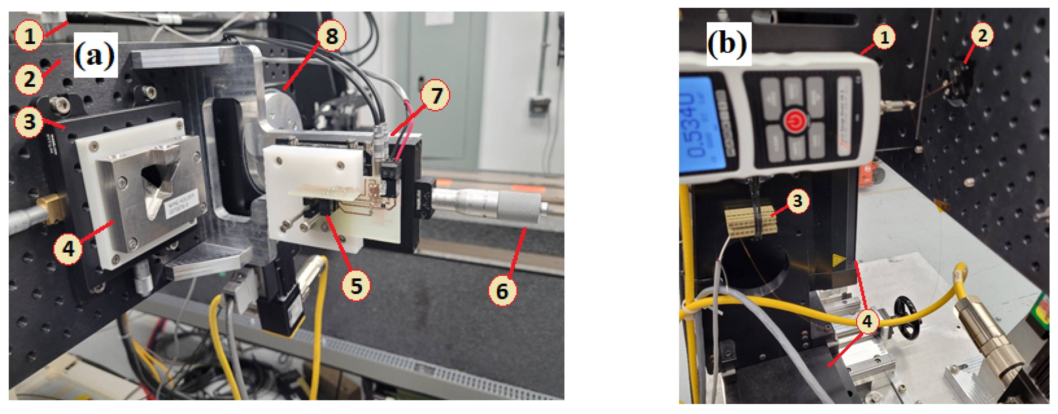
Figure 2.
(a) Experimental setup of test quadrupole. Water-cooled magnet mounted to test stand with manual adjusters for roll/pitch/yaw. Hall probe fed through magnet with bend at end of arm. (b) B field from Hall probe measurement through quadrupole, off-axis for nonzero field, with flat-top field profile indicating negligible roll/pitch/yaw between quadrupole and Hall probe system. and are offset in this plot because the measurement was not taken equidistant in Y and X from the quadrupole center.

Figure 3.
(a) Optical switch position calibration curves (horizontal wire position only) with repeatability test over narrowed region of interest. Dashed box shows region of interest. (b) Zoom around narrowed region of interest with solid red lines showing linear fits to four repeatability trials.
Figure 3.
(a) Optical switch position calibration curves (horizontal wire position only) with repeatability test over narrowed region of interest. Dashed box shows region of interest. (b) Zoom around narrowed region of interest with solid red lines showing linear fits to four repeatability trials.

Figure 4.
Measurement of the n=10 wire harmonic using a B field from a spare quadrupole magnet. (a) Wire amplitude and phase (of wire motion relative to drive current) measured at lock-in amplifier, where markers show the average value of 40 samples taken 0.1 sec apart and error bars show standard deviation of same. (b) curve computed from wire amplitude and phase, where error bars show standard deviation by error propagation; solid red line shows curve fit and dashed grey line shows inclusion/exclusion (1/0) of points for fit (more discussion later in text).
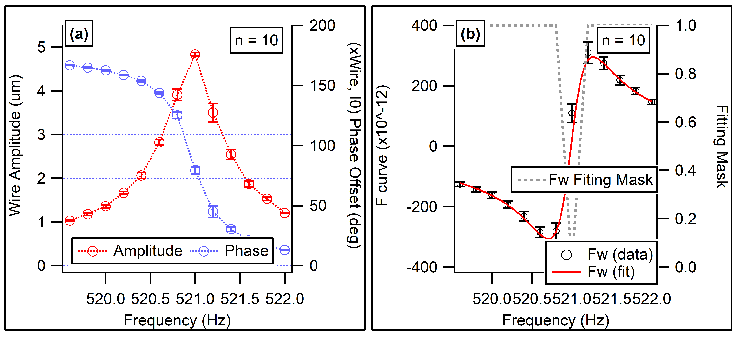
Figure 5.
Vibrating wire precision study, encompassing 340 scans of the n=10 harmonic, plotting measured wire resonant frequency (divided by harmonic number) versus ambient temperature. Marker shape indicates measurement date and marker colour indicates chronology: red scans earlier in the day, blue scans later in the day.
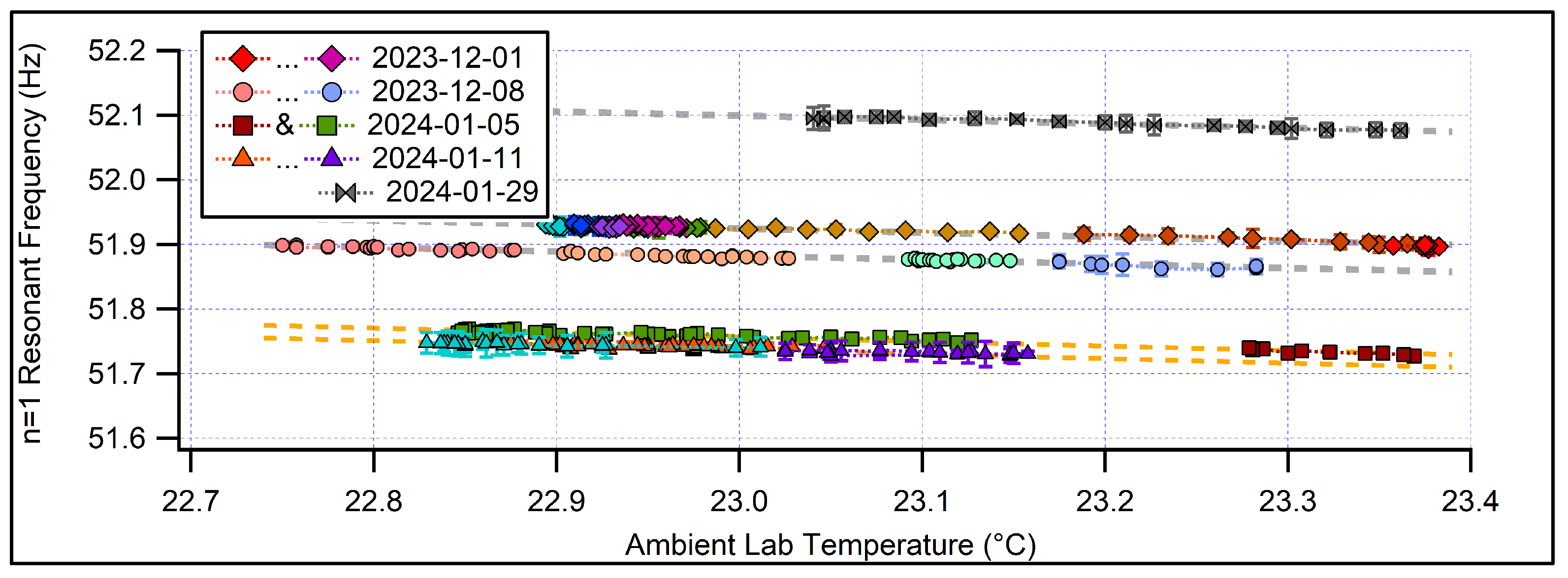
Figure 6.
Vibrating wire precision study, encompassing 340 scans of the n=10 harmonic, plotting measured strength of the Sine coefficient versus ambient temperature. Marker shape indicates measurement date and marker colour indicates chronology: red scans earlier in the day, blue scans later in the day.
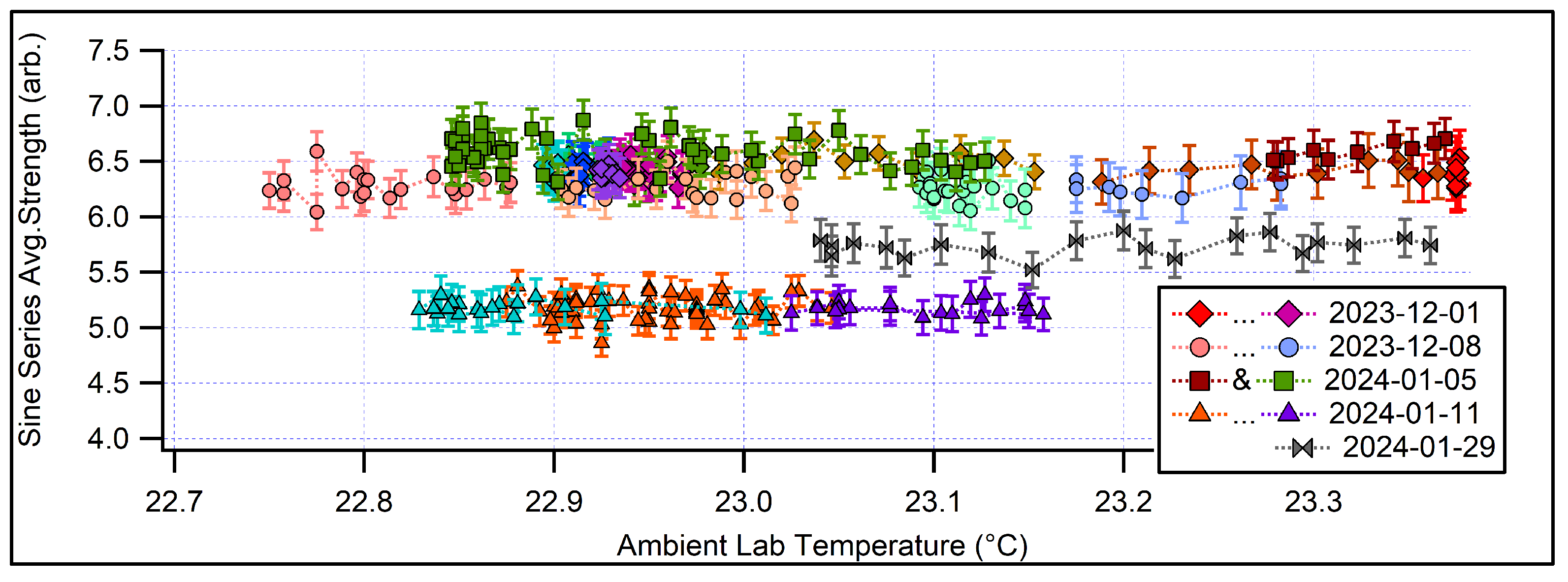
Figure 7.
Scatter plot comparison of the Sine coefficient from repeated simultaneous measurements using horizontal ( field) and vertical () wire detector switches. Offsets in data ascribed to shifts of the detector assembly between measurement days. Colored boxes indicate estimated uncertainty in and of select representative scans.
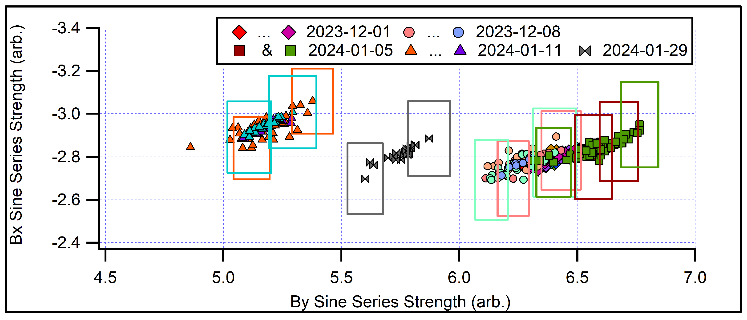
Figure 8.
Typical frequency response measurements for 86 wire harmonics from n=1...114, with n=46 in bold-solid as a representative sample and n=59 in bold-dashed as an unusually broad peak. Symmetric shape and absence of sudden amplitude collapses indicate wire motion was non-hysteretic. Highlighted regions indicate ± wire phase, which coincided with peak wire amplitude.
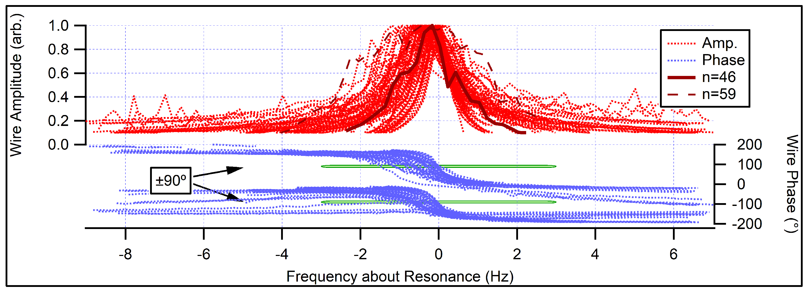
Figure 9.
Atypical frequency response measurements for 90 wire harmonics, batched into three characteristic profiles. Darker bolded traces indicate a representative scan. (a)/(b) Measurements where wire amplitude was asymmetrically stronger below/above wire resonance. (c) Scans where wire amplitude dipped above a weakly defined resonant peak. Highlighted regions indicate ± wire phase, which often did not coincide with peak wire amplitude.
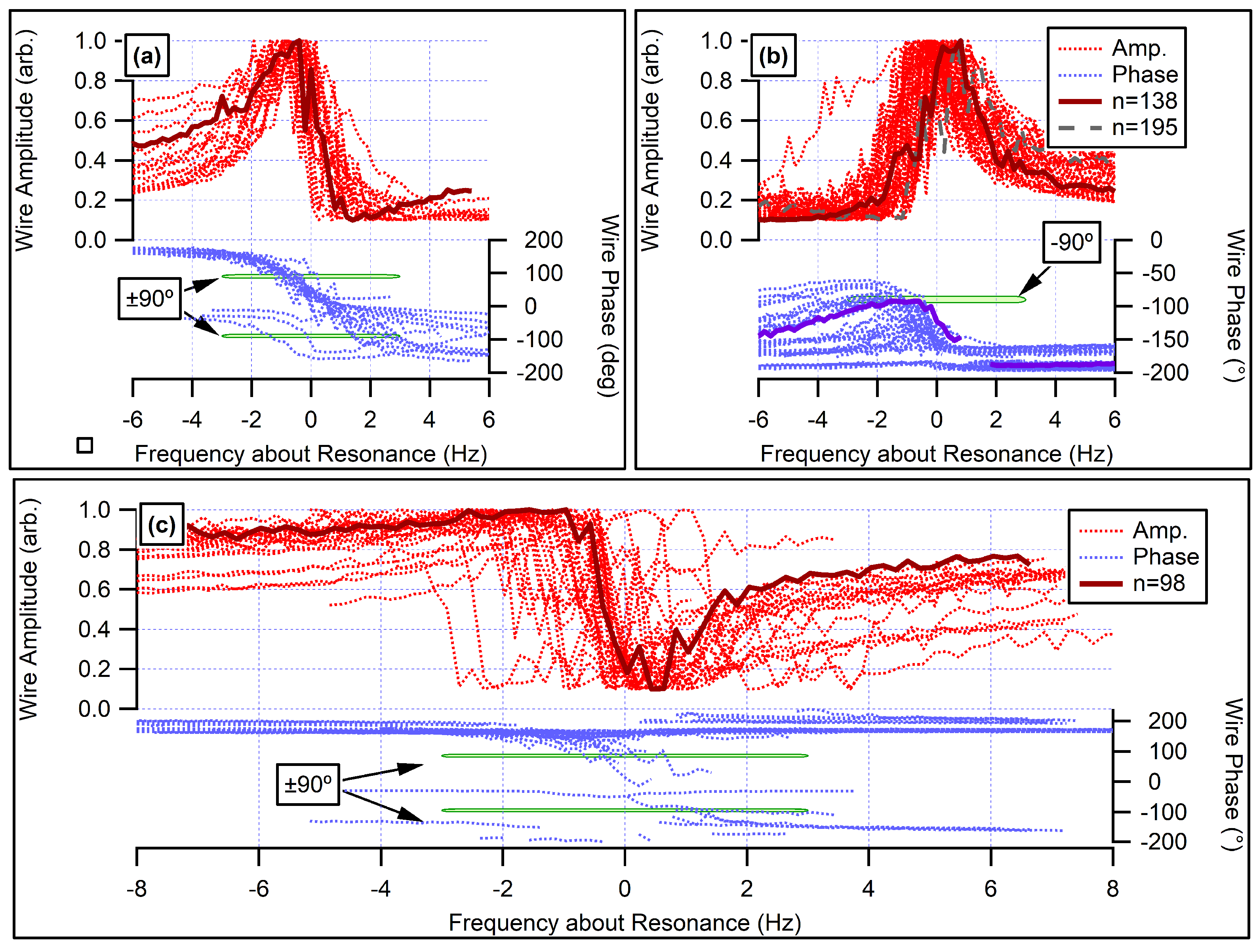
Figure 10.
Measured frequency response of wire amplitude in both planes for select harmonics. (a) Cases of positive correlation. (b) Resonant horizontal motion correlated with suppressed vertical motion. (c) Resonant vertical motion correlated with suppressed horizontal motion. (d) Suppression in both planes for the same harmonic.
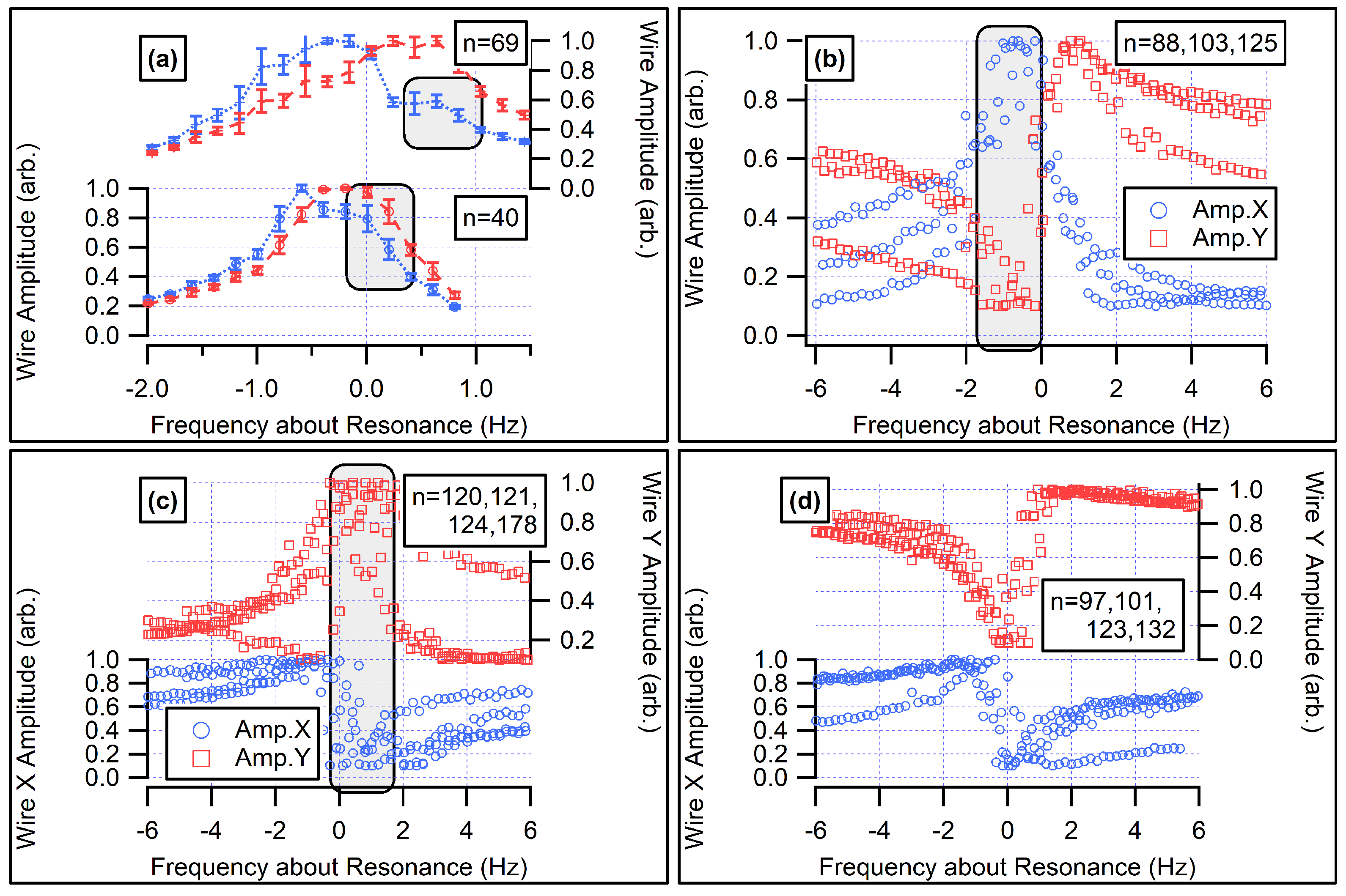
Figure 11.
Behaviour of (, , ) curve fitting coefficients across n=200 vibrating wire scans of a test magnet. (a) Fundamental frequency of wire via coefficient. (b) Wire damping via coefficient. (c) offset correction coefficient. (d) Scatter plot showing correlation of against .
Figure 11.
Behaviour of (, , ) curve fitting coefficients across n=200 vibrating wire scans of a test magnet. (a) Fundamental frequency of wire via coefficient. (b) Wire damping via coefficient. (c) offset correction coefficient. (d) Scatter plot showing correlation of against .
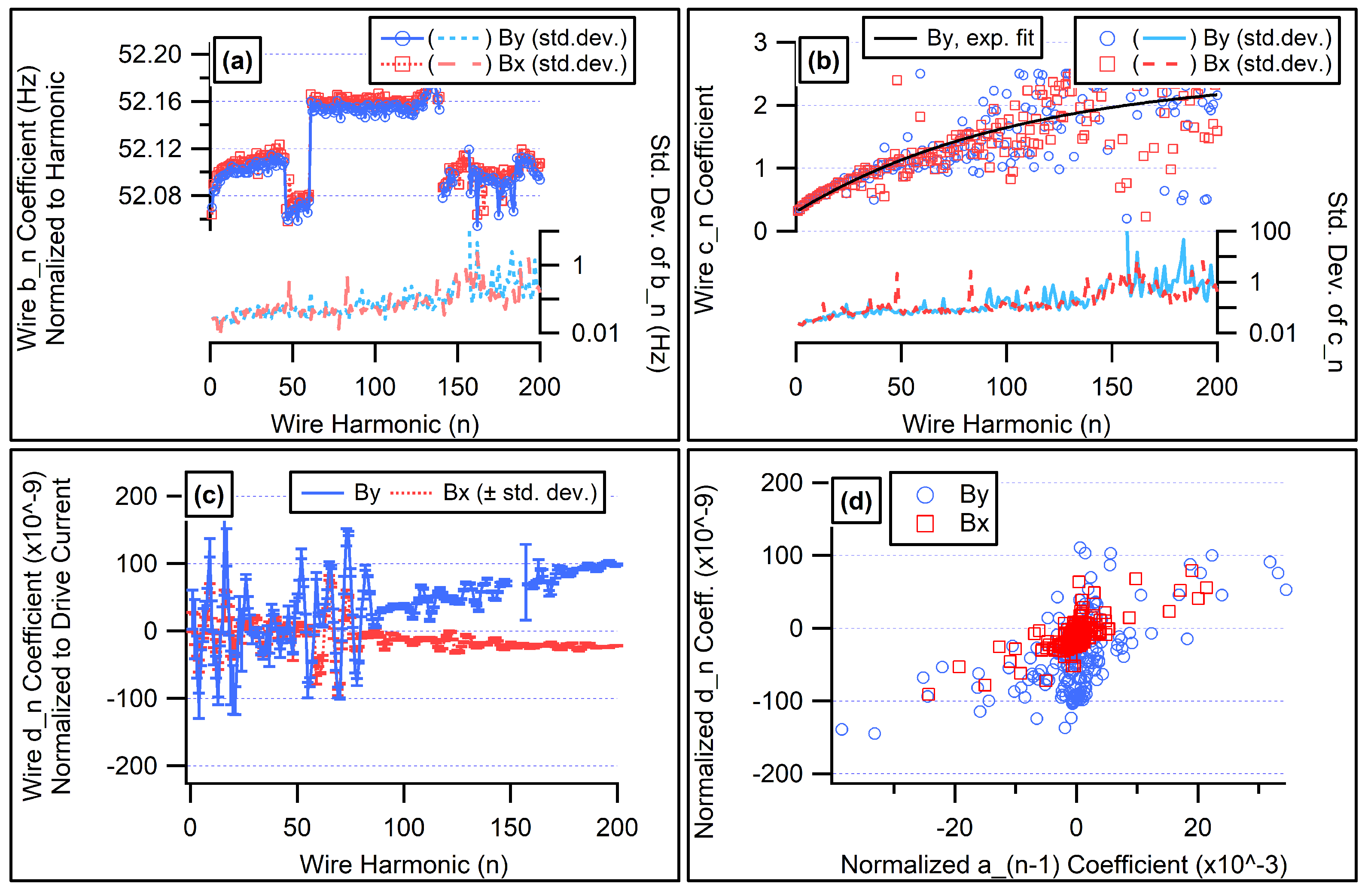
Figure 12.
Measured vibrating wire Sine coefficients (n=1,2..200 harmonics) and DST of reference Hall probe scan measured at common positions relative to magnetic center of a test quadrupole with and field components. (a) First 50 harmonics for and (b) latter harmonics (note reduced vertical scale). (c) and (d) show same for .
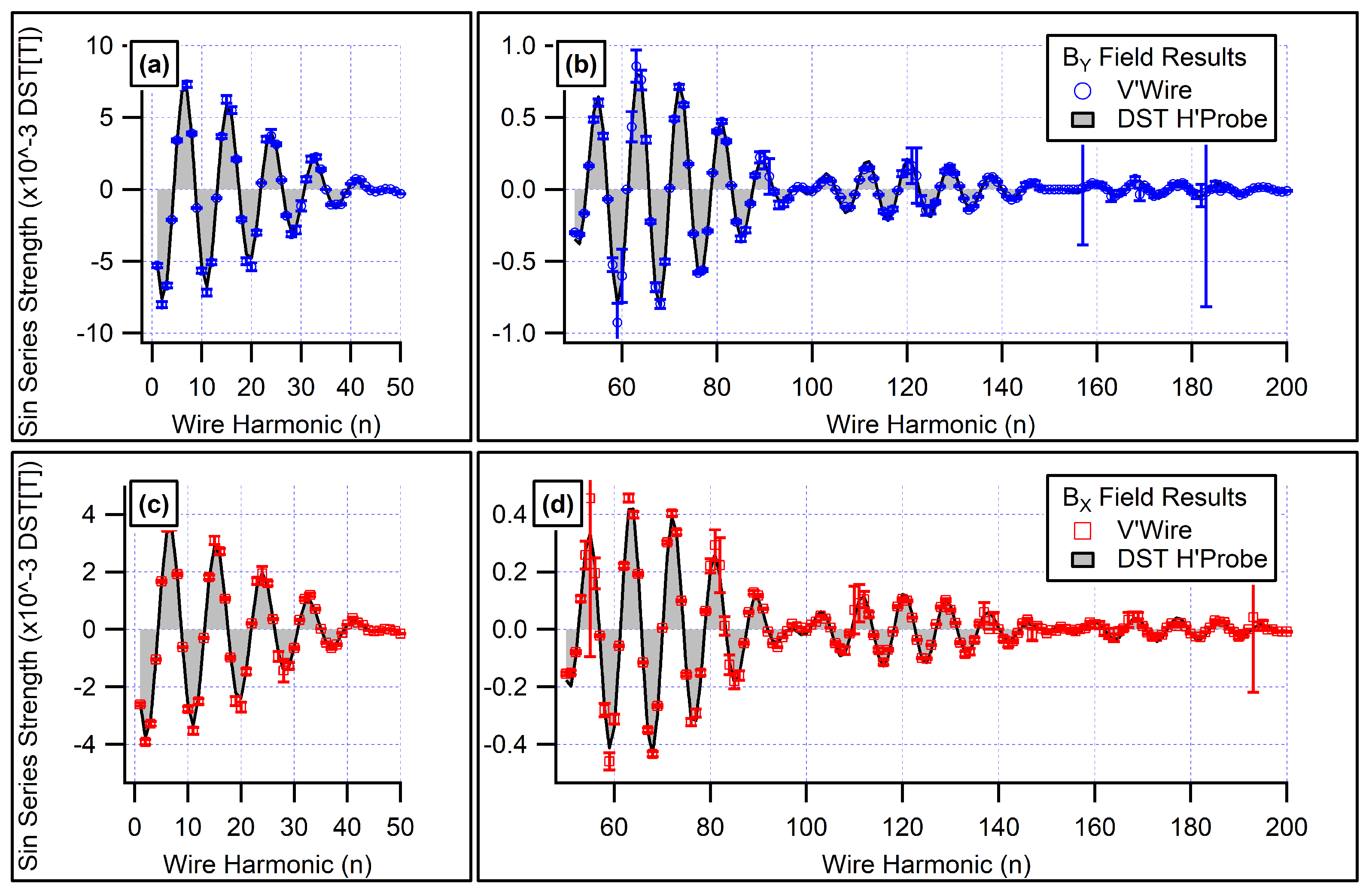
Figure 13.
B field reconstructed from vibrating wire measurements (up to n=200 harmonics) together with reference Hall probe scan (dashed). and field components. Vibrating wire shown with (solid) and without (dotted) empirical scalar corrections. (a) Horizontal zoom in region of magnetic field. (b) Vertical zoom across full wire length.
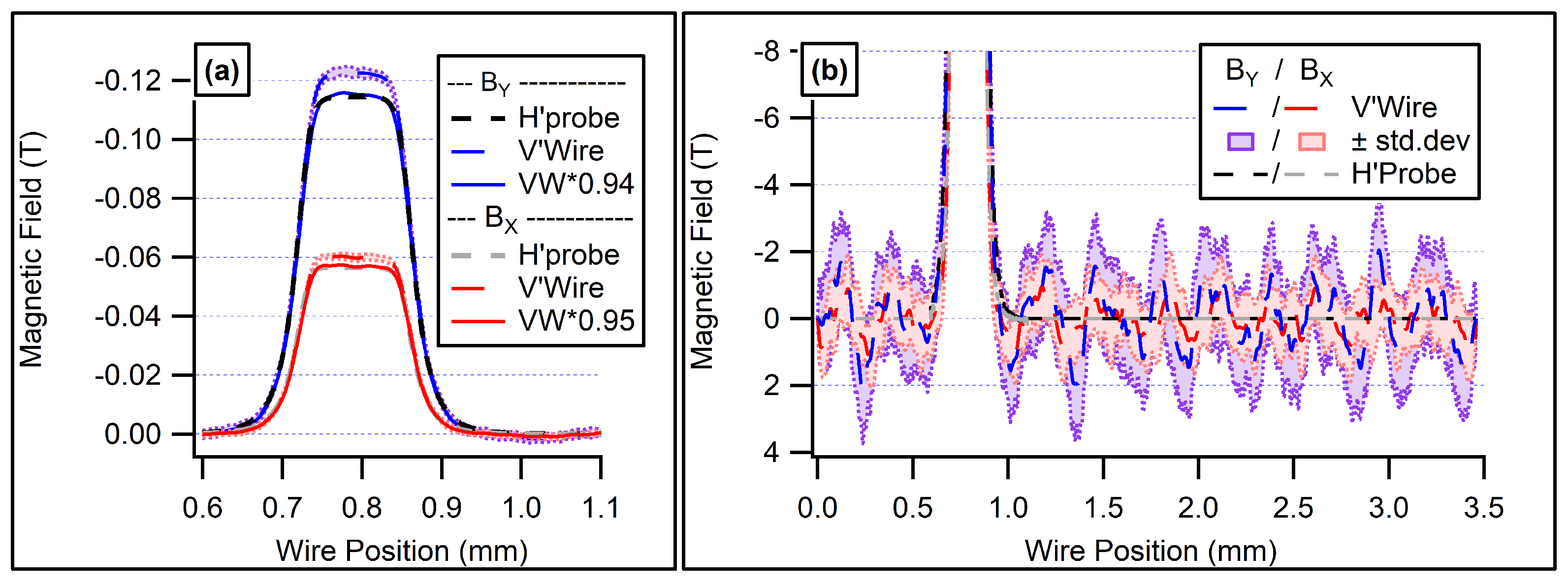
Figure 14.
Scatter plot summary of relative agreement between n=200 Sine series coefficients obtained by vibrating wire scan compared against DST of reference Hall probe scan. Empirical scalar corrections (on the order of 5%) applied to vibrating wire data to address calibration/gain error. and field components measured simultaneously.
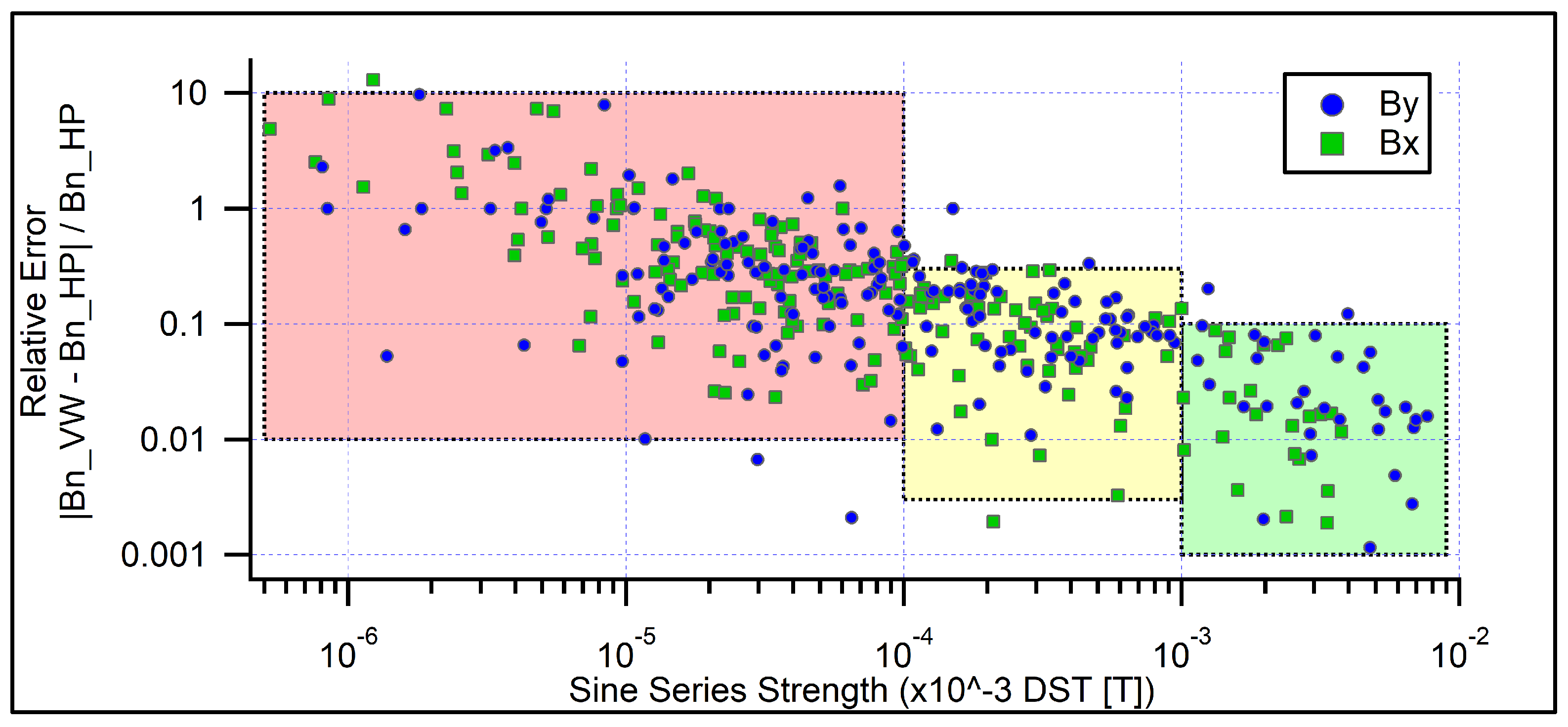

Table 1.
Nominal, low, and high settings for vibrating wire scan parameters varied throughout precision study of the n=10 harmonic.
Table 1.
Nominal, low, and high settings for vibrating wire scan parameters varied throughout precision study of the n=10 harmonic.
| Scan Parameter | Nominal | Low | High |
|---|---|---|---|
| Frequency step (Hz) | 0.2 | 0.1 | – |
| Wire drive current (pk mA) | 0.25 | 0.15 | 0.5 |
| Settling time (s) (mA) | 4.5 | – | 7 |
| Read delay (s) | 0.1 | – | 0.3 |
| Lock-in sensitivity (µV) | 500 | 200 | – |
| Lock-in time constant (ms) | 100 | – | – |
| Samples averaged/point | 15 | 1 | 100 |
Table 2.
Mean and standard deviation of the Sine coefficient across 340 vibrating wire scans, batched by measurement day, to compare results with and without masking data near wire resonance.
Table 2.
Mean and standard deviation of the Sine coefficient across 340 vibrating wire scans, batched by measurement day, to compare results with and without masking data near wire resonance.
| Measurement | N. Scans | Fit to full curve | Masking 90 ± data | % Drop | ||
|---|---|---|---|---|---|---|
| Date | Mean | SDEV | Mean | SDEV | in SDEV | |
| 2023-12-01 | 100 | 6.42E-03 | 7.89E-05 | 6.42E-03 | 6.58E-05 | 17 |
| 2023-12-08 | 70 | 6.27E-03 | 1.04E-04 | 6.26E-03 | 7.49E-05 | 28 |
| 2024-01-05 | 60 | 6.59E-03 | 1.27E-04 | 6.59E-03 | 9.65E-05 | 24 |
| 2024-01-11 | 90 | 5.18E-03 | 8.88E-05 | 5.18E-03 | 7.62E-05 | 14 |
| 2024-01-29 | 20 | 5.73E-03 | 8.67E-05 | 5.75E-03 | 6.79E-05 | 22 |
Table 3.
Mean and standard deviation of the Sine coefficient across three 20-scan trials from 2024-01-11, batched by number of samples averaged per frequency step, with and without masking data near wire resonance. Standard deviation values also listed normalized to N=1 sample per step.
Table 3.
Mean and standard deviation of the Sine coefficient across three 20-scan trials from 2024-01-11, batched by number of samples averaged per frequency step, with and without masking data near wire resonance. Standard deviation values also listed normalized to N=1 sample per step.
| N. | Fit to full curve | Masking 90 ± data | ||||
|---|---|---|---|---|---|---|
| Samples | Mean | SDEV | Rel. SDEV | Mean | SDEV | Rel. SDEV |
| 1 | 5.20E-03 | 9.37E-05 | 1.00 | 5.21E-03 | 7.74E-05 | 1.00 |
| 50 | 5.17E-03 | 5.46E-05 | 0.58 | 5.17E-03 | 6.04E-05 | 0.78 |
| 100 | 5.18E-03 | 5.54E-05 | 0.59 | 5.18E-03 | 5.24E-05 | 0.68 |
Table 4.
Mean, standard deviation (SDEV), and coefficient of variation (CV) of the Sine coefficient across 340 vibrating wire scans, batched by measurement day, for simultaneous and field measurements. Sine coefficients calculated with data near wire resonance masked from curve fits.
Table 4.
Mean, standard deviation (SDEV), and coefficient of variation (CV) of the Sine coefficient across 340 vibrating wire scans, batched by measurement day, for simultaneous and field measurements. Sine coefficients calculated with data near wire resonance masked from curve fits.
| Measurement | Mean | SDEV | CV (%) | |||
|---|---|---|---|---|---|---|
| Date | ||||||
| 2023-12-01 | 6.42E-03 | -2.80E-03 | 6.58E-05 | 2.84E-05 | 1.02 | 1.02 |
| 2023-12-08 | 6.26E-03 | -2.76E-03 | 7.49E-05 | 6.27E-05 | 1.20 | 2.27 |
| 2024-01-05 | 6.59E-03 | -2.84E-03 | 9.65E-05 | 3.91E-05 | 1.47 | 1.38 |
| 2024-01-11 | 5.18E-03 | -2.94E-03 | 7.62E-05 | 4.07E-05 | 1.47 | 1.39 |
| 2024-01-29 | 5.75E-03 | -2.81E-03 | 6.79E-05 | 4.10E-05 | 1.18 | 1.46 |
Disclaimer/Publisher’s Note: The statements, opinions and data contained in all publications are solely those of the individual author(s) and contributor(s) and not of MDPI and/or the editor(s). MDPI and/or the editor(s) disclaim responsibility for any injury to people or property resulting from any ideas, methods, instructions or products referred to in the content. |
© 2025 by the authors. Licensee MDPI, Basel, Switzerland. This article is an open access article distributed under the terms and conditions of the Creative Commons Attribution (CC BY) license (http://creativecommons.org/licenses/by/4.0/).
Copyright: This open access article is published under a Creative Commons CC BY 4.0 license, which permit the free download, distribution, and reuse, provided that the author and preprint are cited in any reuse.


