Submitted:
21 April 2025
Posted:
22 April 2025
You are already at the latest version
Abstract
This paper investigates the impact of income inequality on CO2 emissions in Malaysia. It also tests the environmental Kuznets curve (EKC), covering the period from 1989 to 2023. The Error Correction Model (ECM) and Autoregressive Distributed Lag (ARDL) bounds testing techniques are used in the study to evaluate the short- and long-term relationships between variables. The empirical results obtained from the analysis support the EKC hypothesis. Besides, the results indicate that income inequality and other control variables such as, energy consumption, and industrialization have a positive relationship with carbon dioxide, while urbanization has an insignificant negative connection with CO2 emissions. The findings are reliable, consistent, and robust as they are tested using several stability and diagnostic procedures. The study's conclusions may significantly impact Malaysia's ability to implement appropriate policies to cut CO2 emissions.
Keywords:
Carbon Dioxide Emissions
; Environmental Kuznets Curve
; Gross Domestic Product
; Income Inequality.
1. Introduction
Social and environmental issues are commonly acknowledged to be two of the world’s most pressing challenges (Knight et al., 2017). Currently, the environmental deterioration and the rising rate of wealth disparity are the big worries in many nations(Baloch, Danish et al., 2020). According to Mcgee and Greiner, 2018 rise in income would increase environmental degradation in countries with low-income equality. Still, the relationship would be the opposite in countries with higher income equality. Meanwhile, numerous researches suggest that lower income inequality plays a key role in environmental protection, which can contribute to extreme poverty (Cho, 2018). Barbier, 2010 believes that fair environmental conditions are essential for health. The absence of a proper environment can lead to higher fatality rates, especially in low-income societies (Barbier, 2010). A decline in extreme poverty may decrease the rate of environmental degradation, as lower-income societies highly depend on natural resources, leading to higher environmental degradation. The direct connection between poverty and environmental degradation causes depletion and misuse of natural resources, resulting in more pollution and lower quality of the environment (Munasinghe, 1999). In addition to extreme poverty, other factors, such as a high rate of urbanization and population, are known to hurt both natural resources and environmental quality (Rai, 2019).
Siwar and Murad (2001) reported that economic activities in Malaysia are highly centralized in urban areas of the country. The unbalanced population growth in metropolitan areas triggered unplanned housing and overcrowding and caused poor household waste management and other environmental concerns. Although Malaysia has made significant progress regarding solid waste management after introducing eco-friendly policies, there are still major concerns in cheaper residential areas and areas where squatters live. Hence, comprehensive policies and procedures must address these concerns across urban areas (Murad & Mustapha, 2010). Besides solid wastes, which are creating environmental upsets, CO2 emissions, and climate changes are also challenging the country. The increasing rate of CO2 raises the temperature and aggravates climate change, which can lead to several health problems, including cardiac and respirational diseases. Reducing air pollution could prevent 5900 early deaths annually in Malaysia after 2030 (WHO, 2015).
One of the reasons behind this is that Malaysia relies heavily on fossil fuels for electricity production (Basri et al., 2015). Meanwhile, fossil fuel is not the only contributor to CO2 emissions; other factors such as urbanization, population, economic activities, income distribution, and many others also play their role in terms of increasing the rate of CO2 emission (Wolde-Rafael & Idowu, 2017; X. Wang et al., 2020; Yang et al., 2020). Malaysia, among other developing countries, has been experiencing increasing income inequality, which not only leads to several social and economic problems, such as poverty but also causes environmental concerns, such as CO2 emissions in the country (Khalid & Yang, 2021; Yang et al., 2020; Wang et al., 2020).
The trade-off between economic activities and environmental protection is challenging for most developing nations, including Malaysia. To coup with this particular challenge, the government of Malaysia is looking for a reduction of 45% in the rate of greenhouse gas emissions before reaching the year 2030, with this percentage of 35% being an unconditional reduction while the remaining is conditioned upon the availability of climate finance and technological access (Koswanage, 2015). Although there are numerous studies underlining the connection between economic activities and environmental degradation, especially within the context of the environmental Kuznets Curve (EKC), the majority of these studies have obtained inconclusive outcomes due to applying a weak econometric model (Narayan & Narayan, 2010; Dinda, 2004).
Most studies show that income and economic imbalance may affect the health of the environment (Hübler, 2017; X. Wang et al., 2020; Yang et al., 2020). Not including income inequality would cause omitted variable bias when testing the income-environmental degradation nexus (Dogan & Turkekul, 2015; M. A. Baloch, Ozturk, et al., 2020;). The available literature regarding income inequality and environmental degradation is quite diverse (Knight et al., 2017; Hailemariam et al., 2019;). The outcomes of the studies vary across the countries due to differences in their economic conditions across nations; the results are also because of different periods and data types and because of distinct methodologies employed in the studies (Magnani, 2000; Jorgenson et al., 2016; Mittmann & de Mattos, 2020; Bhattacharya, 2019; Uddin et al., 2020; Hubler, 2017)
In this context, a few questions are raised, such as: How does a change in income inequality affect the rate of CO2 emissions? Is there evidence that can support the environmental Kuznets Curve in Malaysia? What is the connection between CO2 and other influencing variables? What policies can lighten the problem of CO2 emissions in Malaysia? This study is designed to explore the impact of income inequality on CO2 emissions from 1989 to 2023 in Malaysia. The study will also look for evidence to test the EKC hypothesis in the country, and it will also test the impact of other determinants of CO2 emissions in both the short run and long run.
It is widely recognized that the surging rate of CO2 emissions is a primary ecological concern worldwide because it is a toxic gas that can harm humans, animals, and plants. Multiple economic and social factors, including unequal income, contribute to the high rate of CO2 pollution. To the author’s best knowledge, no attempt has been made yet to test the income inequality – CO2 emissions nexus along with the EKC hypothesis in Malaysia. The available studies conducted in Malaysia focus on the determinants of CO2 emissions considered the impact of several other variables such as urbanization, energy consumption, foreign direct investments (FDI), financial development, trade openness, and. (see, for example, Hassan et al., 2019; Aslam et al., 2021; Ali et al., 2020; Nurgazina et al., 2021; Shahbaz et al., 2016; Begum et al., 2015). These researchers have excluded income distribution as a factor in EKC studies, which might have a significant impact and is known to have major economic and social implications (Torras & Boyce, 1998; Baek & Gweisah, 2013; Morse, 2018). This paper is the first one the author knows of that examines how income inequality affects CO2 emissions. Therefore, it will fill a significant gap in the research on CO2 in Malaysia and improve knowledge of how wealth distribution and levels affect environmental quality in the country. The findings will help policymakers design and implement effective policies that can address ecological problems, income distribution, and economic growth at the same time. Unlike other related research conducted in Malaysia, the present study applied an accurate method for testing EKC.
The model provides the required and adequate conditions for testing the inverted U-shaped connection between income levels and environmental quality. Most of the research conducted previously in Malaysia applied the quadratic model to confirm the EKC hypothesis or inverted U-shaped relationship, which only met the critical requirement of the hypothesis (Gill et al., 2018; Begum et al., 2015; Ali et al., 2017; Mehraaein et al., 2021). These results are more likely to be misleading because of specification errors and a strong association between the linear and nonlinear series. With a more conclusive model that includes several necessary variables, we hope to obtain more precise and accurate results from the current study. Considering the lack of enough research to simultaneously describe the validation of EKC and the connection between income inequality and CO2 emissions in Malaysia, this study has been carried out to bridge this gap and provide proper recommendations to parties working in relevant areas. Finally, the study would also provide information on the contribution of other influencing variables to CO2 so that policymakers can understand the variables with the highest and the lowest contribution to CO2 emissions in the country.
This paper contains five sections. The first section starts with the introduction, followed by the objectives, the novelty, and the organization of this paper. The second section gives background information on some significant economic, social, and geographical indicators of Malaysia. However, the fourth section includes theoretical and empirical literature, which describes the theoretical and empirical analysis of the nexus between income inequality and CO2 emissions in different countries. The fifth section describes the methodology of the study. This section explains the data, variables, and techniques used in the analysis. Finally, the research ends with section six, which explains the results and the discussion. This section ends with a comprehensive conclusion, recommendations, limitations of the study, and directions for future studies
2. Background of the Study
2.1. CO2 Emission in Malaysia
Understanding the importance of tackling climate damage, Malaysia voluntarily targeted a decline in GHG emissions from GDP growth by 2020 (Begum et al., 2015). The energy intensity was reduced under the 10th Malaysia plan by 33 % in 2013, although less than the reduction target. To mitigate greenhouse gas pollution and to produce enough sustainable energy, Malaysia would have to invest large amounts of money in renewable energy. Malaysia has vast clean energy resources, such as palm oil biomass residues, mills, solar, urban waste, landfill gas, hydro, and rice (Gill et al., 2018). Malaysia has been taking advantage of energy resources associated with the high level of CO2 emission. As is displayed in Figure 1, the country has been experiencing an upward trend in CO2 emissions. As per the chart, CO2 is calculated in metric tons per capita through 1988 and 2018. The data indicates that in the late 1980s, carbon dioxide emissions were less than three metric tons per capita. Since then, it had increased continuously until 2008, reaching almost 7.5 metric tons per capita. Although the emissions declined from just below 7.5 in 2008 to almost 6.5 in 2009, they started to rise at a fluctuating rate again after 2009 and reached a peak of more than in 2014.
2.2. Income Inequality in Malaysia
income inequality is not the same for all countries globally, as the geographical, social, economic, and political conditions for all the countries are not the same. Among these countries, Malaysia is one of the fast-developing nations that has also been experiencing an increasing rate of income inequality for a long time. It is assumed to be the leading cause of the political uprisings in 1969, which made ground for the presentation of the New Economic Policy (NEP) between 1971 and 1990. The National Development Policy (NDP) and the National Vision Policy (NVP) for 1991 – 2000 and 2001 – 2010 designed the NEP supporting the growth strategy with equality. Attaining a high level of economic progress and income equality was the main goal of the NEP. The goal was accomplished quite well because the country has experienced economic growth and income redistribution. The significant growth of the manufacturing sector triggered economic growth with an average annual rate of 6.4 percent over thirty-five years since 1970 (RAGAYAH, 2008).
Meanwhile, the strategy was also successful in controlling the income inequality in the country, as shown in Figure 2, which describes the rate of income inequality over three decades, from 1987 to 2018. Overall, the graph suggests a downward trend in the rate of income inequality, which means that the country has experienced a decline in income inequality. According to the graph, in 1989, the rate was more than 46%, reaching a peak value of almost 51% in 1994. Since then, the country has continued to experience a plunging rate of income inequality until 1999, when it reached almost 44%. The rate started to surge, fluctuating after 1999, and reached almost 49% in 2007.
Meanwhile, the country started to go through a sharp decline in income inequality after 2007. Finally, the rate was just above 42% in 2018. The trend for the rate of income inequality was also similar in rural and urban areas during the period of the NEP. The rate of income inequality represented by the Gini coefficient went up in rural areas during 1970 and 1976. However, it went down to 0.409 by the year 1990. Likewise, the Gini coefficient for urban areas also went in the same direction between 1970 and 1976. However, the rate of income inequality in urban and rural areas differed during the 1990s. The Gini coefficient continued to increase in rural areas between 1990 and 1997. After 1997, the rate of inequality started to decline and reached a low level of 0.397 in 2004. Meanwhile, the rate dropped in urban areas between 1990 and 1999, after which the Gini coefficient increased. In 1997, the average income of the urban individuals in the group of the top 20% increased to RM 8750, which dropped by 10.5% between 1997 and 1999 (Ragayah, 2002).
3. Theoretical background
3.1. Impact-Population-Affluence-Technology (IPAT) Model
The model is an extension of the “Impact = Population × Affluence × Technology (IPAT)” equation introduced by Ehrlich and Holdren (1971), which takes population, income level, and technology as key contributors to environmental quality. The IPAT model is mostly criticized because of measuring the technological impact of the emission-to-GDP ratio, which is not only affected by technological progress but can also be influenced by several other factors that are not part of the model Dietz, T., & Rosa, E. A. (1994). Besides, the IPAT model is only restricted to demographic and economic factors; it excludes other variables (Scholz, 2006). The model is also criticized because of certain principles of accounting, which assume a proportional connection between environmental degradation and other variables in the model and, thus, does not permit hypothesis testing (York et al., 2003b).
Dietz and Rosa (1994) suggest that using the IPAT identity for hypothesis testing may be challenging. They modified the “Stochastic Impacts by Regression on Population, Affluence and Technology (STIRPAT)” model. The modified version is beneficial because it is more accurate and sensitive to environmental impacts; it can have several extensions and accommodate other variables linked to environmental degradation (York et al., 2003). For Instance, one can decompose the (T) into different variables that are not part of the models (York et al., 2003b). Meanwhile, some studies have also decomposed other variables than T to structure their models and evaluate the impact of specific variables on the environment. (Zhou & Liu, 2016) decomposed P into the working-age population, household size, urbanization rate, and population size. (Dietz & Rosa, 1994; York et al., 2003; Fan et al., 2006; Poumanyvong & Kaneko, 2010; Shahbaz et al., 2016; Mcgee & Greiner, 2018; Yang et al., 2020). This research utilizes it to see how the income inequality affects the environment.
One can specify the model as:
After applying of the natural logarithm to both sides, we can write:
In equation 3.2, where the natural logarithm of all variables has been taken, t represents a period, α stands for constant, P denotes population, A symbolizes economic growth, T stands for technology, and character I is used to indicate the environmental quality, and the error terms is identified with ε. As mentioned, a good characteristic of the STIRPAT model is that one can add additional factors to observe their environmental impact. This is mainly because P, A, and T are decomposable (Dietz & Rosa, 1994). To see the impact of various social and economic factors on the environment, researchers have introduced multiple models by employing different variables in the STIRPAT framework. (Zhou & Liu, 2016) For example, P was divided into the working-age population, household size, urbanization rate, and population size. Likewise, Poumanyvong & Kaneko, 2010 & Wang et al., 2017 employed industrialization and intensity of energy to stand for T in the STIRPAT framework. Moreover, numerous studies indicate that the environmental Kuznets Curve hypothesis can be supported for several countries (Grossman & Krueger, 1991; Panayotou, 1993; Lazăr et al., 2019; Uzar & Eyuboglu, 201). Hence, we are adding the square of economic growth in our STIRPAT model to look for evidence regarding the EKC hypothesis in Malaysia. To obtain relatively unbiased results, several researchers have also added trade openness as a control variable to their model (Shahbaz, Lean, & Shabbir, 2012; Ling et al., 2015 Ahmad, Shahbaz, and Kyo, 2016). The rise in trade openness increases economic activities, which leads to higher consumption and production of goods and services. As these activities lead to pollution, one might conclude that trade openness increases environmental degradation. Finally, several studies across the globe also found income distribution as a key determinant of environmental quality (X. Huang et al., 2012; Uddin & Smyth, 2014; Zhang & Zhao, 2014; Grunewald et al., 2015; Ali et al., 2016; Bae, 2018; Liu et al., 2019; You et al., 2020; Alegre, 2020; Kusumawardani & Dewi, 2020; Z. Huang & Duan, 2020; Granser, 2021).
3.2. Environmental Kuznets Curve (EKC) Hypothesis
This section reviews previous research and information on economic activities and environmental quality, focusing on the EKC. According to Yang and Chng (2021), environmental degradation is connected to various phases of economic growth. The nature of degradation changes as countries grow, and the need for further economic growth influences the shape of the environmental degradation curve. Hence, looking only for economic growth will harm the environment (Bissoon, 2018).
Grossman and Krueger (1991) found enough evidence to support the inverted U-shaped connection between environmental degradation and economic growth. In other words, their study ended with the same results as Kuznets’s (1955) theory suggests. Simon Kuznets introduced the theory. Hence, the Environmental Kuznets Curve (EKC) suggests an inverted U-shaped relationship between economic activities and environmental quality. The EKC theory was modified later by various scholars such as Grossman and Krueger (1991) and Shafik and Bandyopadhyay (1992). They tried to adjust the theory by adding several other variables, including Income inequality. (Figure 3).
The graph describes the EKC theory in three stages of economic development: the first is before industrial activities, the second is in the industrial phase, and the last is in the post-industrial stage. As per the graph, the impact of income is different in each of the three phases. As per the theory, in the pre-industrial stage or throughout the early stage of development, an increase in income leads to lower quality of the environment. The rising income continues to increase environmental degradation until reaching a certain point at stage two. After reaching the peaking point, an increase in income is believed to improve the quality of the environment (Ginevicius et al., 2017). In the first phase of economic development, as industrialization blooms, the agriculture sector grows, and resource extraction increases, the depletion of resources also rises along with waste generation (Dinda, 2004). After reaching the second stage of economic development, as the economy industrialized and started supplying capital goods, pollution is expected to grow monotonically with income per capita (Urheim, 2009). At the initial phase of industrialization, where societies are believed to be relatively poor, environmental quality is expected to decrease because people struggle to fulfill their vital food and accommodation needs. Likewise, Dasgupta et al., 2002 stated that in the initial phase of economic development, environmental regulations are not strong enough, and communities are poor and cannot pay for environmental quality. Hence, societies with a low-income level do not allocate more income for environmental protection (Panayotou, 2003). The increased pollution at the initial industrialization stage is considered a tolerable consequence of developing at this particular stage (Arrow et al., 1995). Unlike the first stage, besides increasing income levels, people also pay attention to environmental protection in later phases of economic development.
Hence, environmental regulation becomes more operative, resulting in low environmental degradation (Dietz et al., 2012; Hervieux & Darne, 2015). Affluent societies prefer to buy eco-friendly goods and support strict standards for environmental protection (Dinda, 2004). Grossman and Krueger (1995) believe that high-income nations practice stricter environmental standards than countries with middle- and low-income levels. Finally, at the third or last industrialization phase, the post-industrial stage of economic development, an increase in output results in a better environment due to escalated demand for an improved environment and fundamental changes toward the tertiary sector (Panayotou, 2003). Societies transform from the resource-oriented industrial sector to the light manufacturing and services sector, which decreases emissions levels. According to Stern, 2004, with increased income levels, people became more educated regarding the undesirable impacts of environmental degradation. Generally, industrialized countries adopt relatively strict policies to protect the environment. Hence, these countries experience a decline in environmental degradation.
3.3. Income Inequality and Environmental Degradation
There are various contradicting perspectives in the theoretical and empirical literature on income inequality and environmental quality, which can be summarized in three different approaches. The first one is the political economics approach (PEA). This approach gives attention to power dynamics, which impact environmental policies. This approach looks into environmental protection practices to see if they favor a specific party. The approach also aims to identify which party advocates for environmental safeguarding through political demands, and it tries to find ways to manage conflict among parties and provide effective environmental policies (Boyce, 1994; Torras & Boyce, 1998). Another approach that describes the connection between income inequality and environmental degradation looks into the marginal propensity to emit (MPE) and the economic behavior of households rooted in households’ utilization of goods and services (Ravallion et al., 2000; Heerink et al., 2001; Berthe & Elie, 2015). Ravallion et al., 2000 state that the impact of income inequality depends on the nature of the connection between income and CO2 emission. The reason behind this is that the MPE varies across different income levels. In a poor society where dwellers have a high rate of MPE, rising income inequality will lead to a better environment. The impact can be more noticeable when the income of the poor class of societies surges in low-income countries because this part of the society does not have access to eco-friendly energy, and an increase in income will result in higher MPE. Finally, the income inequality-environment nexus can be described with the approach of Emulation Theory (ET) (Jorgenson et al., 2017; Grunewald et al., 2017). According to ET theory, substantial income disparity impacts social class consumption. People from the low-income class spend more to mimic high-class spending behavior. Hence, they spend most of their income on goods and services with a great pollution rate, which leads to more environmental degradation (Veblen, 1899). Besides, more working hours in countries with significant income disparity will increase household spending and energy demand, increasing environmental degradation (Jorgenson et al., 2017).
Similarly to the theoretical debate, the empirical literature results present various scenarios worldwide (Ajide et al., 2022; Rai et al., 2022; Idrees et al., 2022).
One can categorize the available studies into three groups, considering the varying outcomes. The first one implies that income inequality will lead to good environmental conditions. The second introduces income inequality as a harmful environmental factor, and the last group of studies leads to no significant association between income inequality and the environment. Uzar and Eyuboglu, 2019, for example, undertook research in Turkey to see if there was a connection between income inequality and CO2 emissions where the author employed the ARDL to evaluate time-series data from 1984 to 2014 on CO2 emissions, financial development, the Gini coefficient, per capita GDP, urbanization, and industrialization. They found that variables are co-integrated, and income inequality is directly associated with CO2 emissions.
In contrast, Kusumawardani and Dewi, 2020) found that income inequality negatively impacts CO2 emissions. They also discovered evidence supporting Indonesia’s Environmental Kuznets Curve (EKC). Baloch et al. (2017) also examined the same relationship in Pakistan, where they found income inequality to bring environmental degradation in both short and long periods, and the study did not find evidence that supports the EKC theory. At the same time, Ridzuan et al. (2017) conducted research for ASEAN-4 countries. They obtained results that suggest a negative income inequality-environmental degradation relationship in Malaysia but a positive connection in Thailand in both long and short period.
4. Method
This study uses the Autoregressive Distributed Lag bounds ARDL cointegration method and Error Correction Models (ECM) to test long- and short-run relationships. The best thing about the ARDL approach to co-integration is that it is not linked to the order of integration Pesaran et al., 1996 (2001); it requires all series to be either integration of order zero or I (0) or integration or order one I (1) or combination of them (Quattara,2004; Narayan & Narayan, 2010). Hence, we need a unit root test to check the order of integration before analyzing the ARDL approach. Besides, the ARDL model is a good option due to its effectiveness in analyzing small samples of data and its ability to reduce the concern of autocorrelations and omitted variables (Narayan,2004).
4.1. Empirical Model
The function for the modified version of our STIRPAT model will be as follow:
In the model, refers to CO2 emissions measured in metric tons, stands for Gini coefficient, stands for GDP per capita in USD, denotes population size, represents urbanization, stands for energy consumption, is used for industrialization and is a symbol of trade openness. In the equation 4.1, CO2 emissions act as a dependent variable; others are independent variables, which have been generally known as essential determinants of CO2 emissions by many scholars (See, for example; X. Huang et al., 2012; Uddin & Smyth, 2014; Zhang & Zhao, 2014; H. S. Ali et al., 2016; Wolde-Rafael & Idowu, 2016; Bae, 2018; You et al., 2020; Sager, 2019; Uzar & Eyuboglu, 2019; Alegre, 2020; Kusumawardani & Dewi, 2020; Baloch et al., 2020). The unrestricted error correction model (UECM) of the ARDL approach for the version of the STIRPAT model will be
This study takes natural logarithm of all variables. In other words, we employ a log-log model for a meaningful interpretation of the results. Taking natural logarithms is mainly because the variations in time series data might not be stable due to instability in the series and the fluctuating mean (Asteriou & Hall, 2011 & Baloch et al., 2017). In the equation, βi, ηi, γi, θi, μi, ϕi, ωi, ψi, φi are the dynamic coefficients in the short-run, and δi (i=1,2,3, …, 9) represent the long-run relationship among series in the ARLD approach.
For short-term relationships between the factors, we use the Error Correction Model along with tests for co-integration. The original model proposed by Sargan in 1974 is meant to explain the short-run dynamics of ARDL. The model’s specifications are as follows:
In equation 4.3, λ denotes the speed of adjustment, whereas signifies the error correction term, representing the residuals derived from the preceding co-integration equation. Furthermore, represents the errors in the model. The error term, , is presumed to be identically independent and normally distributed. The adjustment speed (λ) indicates the rate at which the variables revert to the long-term equilibrium.
4.2. Data
Data used in the study spans from 1989 to 2023. Each variable’s data comes from various sources, including World Bank Indicators for Malaysia, the United Nations, and the Organization of Islamic Cooperation (OIC). The limited-time interval selected for the data is because the data for all variables are not available over a long period. The chosen time frame, however, is still sufficient to substantiate the findings and offer details about the effects of several factors, such as income disparity, on Malaysia’s CO2 emissions. All of the aforementioned variables are transformed into their logarithmic form. In the new form, the change in each variable is interpreted in percentage
4.3. Estimation Process
In classical regression, numerous time series, especially in economic studies, require variables to be stationary or reverse back to the mean value Asteriou and Hall 2011. If the condition is not fulfilled, the regression results might not be free from biases, leading to an invalid conclusion (Granger & Newbold, 1974; Shahbaz, 2009). Hence, when dealing with any statistical method requiring stationary, one should always employ a unit root test for all series to check their order integration. Since most economic studies series are not stationary, one can use differentiation methods to make them stationary (Nelson, 1982). This study employs Augmented Dickey-Fuller (ADF) tests introduced by Dickey and Fuller (1979) to look for stationary. After testing for unit root, the next important step is indicating the lag length for all the series in the model. Several criteria (Akaike Information Criterion (AIC), Hannan-Quinn Information Criterion (HQ), and Schwarz Bayesian criterion (SBC)) can be employed for the determination of the appropriate lag lengths (Bekele, 2019). As the F-test is more sensitive to the lag order selection, Shahbaz et al. (2015) use the Schwartz Bayesian criteria (SBC) instead of the Akaike information criteria (AIC) to find the right lag length. The most important explanation is that SBC picks the fewest possible delays, whereas AIC chooses the most possible delays (Saboori & Soleymani, 2011).
The cointegration test was used to see if there was a long-term link between the factors. Many other researchers, like Khemili and Belloumi (2018) and Balochistan (2018), used the same method. The F-statistic is compared to two crucial values, the lower and upper bounds, to determine whether a long-term link between the series exists (Pesaran et al., 2001). The lower bound represents critical values for series integrated at order zero or I(0). However, the second one, which is known as the upper limit, is the one that represents the variables that are integrated into order one I (1) in the ARDL model. While a number that is lower than the lower threshold indicates that there is no long-term link between variables, the F-test result that is greater than the upper bound indicates that there is a long-term correlation between the variables. Furthermore, if the value of the F-statistics was found to be inside the two bounds, the results are inclusive, and an alternative co-integration method needs to be employed (Uzar & Eyuboglu, 2019).
A diagnostic test was also conducted to evaluate the model’s resilience and stability to ensure that it could produce an objective estimate. This included employing the Jarque-Bera, Breusch-Godfrey LM, and Breusch-Pagan-Godfrey tests to examine normalcy, zero autocorrelation, and homoscedasticity. Additionally, the CUSUM and CUSUM Square (CUSUMQ) tests were used to assess the model’s stability
5. Results
According to (Narayan et al., 2004), all series should be tested for unit root or order of integration before employing the co-integration method. This is because different co-integration approaches require different stationary assumptions to be fulfilled to obtain accurate results. Since the ARDL model employed in this particular study requires all series to be either I (0) or I (1), the study employs two of the most practical tests (Augmented Dickey-Fuller and Philips-Perron) to check the order of integration and to make it sure that none of the series is I (2) (Quattara, 2004). Table 4.1 reflects the outcomes of ADF unit root tests for all of the series included in the model. The results indicate that all series, excluding energy consumption (LNEt), are stationary at first difference. Hence, the order of integration for LNEt will be zero, denoted as I (0), and for all other series, it will be one, which can be symbolized as I (1). Since no variable has a higher order than two, one can employ the ARDL bound testing approach for these series.

Table 5.
1. Stationary Tests.
| Series | ADF Test | Order of Integration | ||
| ADF Results at Series levelTest statistics | ADF Results at First Difference OrderTest statistics | |||
| t = -1.627197 (Prob. = 0.7569) | t = -5.711574 (Prob. = 0.0004) | I(1) | ||
| t = -3.443368 (Prob. = 0.0651) | t = -6.166262 (Prob. =0.0001) | I(1) | ||
| t = -2.854620 (Prob. = 0.1908) | t = -4.846167 (Prob. = 0.0030) | I(1) | ||
| t = -2.760706 (Prob. = 0.2219) | t = -4.883407 (Prob. = 0.0027) | I(1) | ||
| t= -2.644798 (Prob. = 0.2652) | t = -10.45895 (Prob. = 0.0000) | I(1) | ||
| t = -2.527850 (Prob. = 0.3134) | t = -5.363315 (Prob. = 0.0009) | I(1) | ||
| t = -2.416990 (Prob. = 0.3638) | t= -4.153290 (Prob. = 0.0147) | I(1) | ||
| t = -1.984377 (Prob. = 0.5851) | t = -4.613239 (Prob. = 0.0054) | I(1) | ||
| t = -4.841822 (Prob. = 0.0032) | I(0) | |||
Table 5.
2. Cointegration.
| Critical Value | Lower Bound | Upper bound | |
| 1%5%10% | 2.622.111.85 | 3.773.152.85 | |
| Selected Model | F – statistics | Co- integration | |
| (2,2,2,1,0,2,2,2,0) | 9.4542918 | Yes | |
Table 5.
3 Long-run relationship.
| Variable | Coefficient | Std. Error | t-Statistic | Prob. |
| 3.826246 | 4.990327 | 0.766732 | 0.0075 | |
| -0.187106 | 0.327779 | -0.570829 | 0.0088 | |
| 0.681762 | 0.250041 | 2.726599 | 0.0343 | |
| 0.580648 | 0.178660 | 3.250018 | 0.0175 | |
| 0.020652 | 0.175029 | 0.117992 | 0.0099 | |
| 1.350851 | 0.225586 | 5.988173 | 0.0010 | |
| 0.316447 | 0.065004 | 4.868154 | 0.0028 | |
| 0.191473 | 0.119522 | 1.601992 | 0.0063 | |
| C | 36.38828 | 35.36797 | 1.028848 | 0.3432 |
Table 5.
4. Short-run relationship.
| ECM Regression | ||||
| Case 2: Restricted Constant and No Trend | ||||
| Variable | Coefficient | Std. Error | t-Statistic | Prob. |
| D(LN_CO2 (-1)) | -0.451542 | 0.069558 | -6.491549 | 0.0006 |
| D() | 65.96833 | 6.329155 | 10.42293 | 0.0000 |
| D( (-1)) | 85.67206 | 8.050464 | 10.64188 | 0.0000 |
| D() | 3.264575 | 0.313316 | 10.41944 | 0.0000 |
| D((-1)) | 4.339991 | 0.405508 | 10.70261 | 0.0000 |
| D() | 0.478480 | 0.060770 | 7.873688 | 0.0002 |
| D() | -0.007026 | 0.038483 | -0.182571 | 0.8611 |
| D((-1)) | -0.131811 | 0.037644 | -3.501498 | 0.0128 |
| D() | 0.468336 | 0.055724 | 8.404506 | 0.0002 |
| D((-1)) | -0.337147 | 0.061428 | -5.488468 | 0.0015 |
| D() | 0.059307 | 0.030554 | 1.941063 | 0.0003 |
| D( (-1)) | -0.296009 | 0.038101 | -7.769091 | 0.0002 |
| CointEq (-1)* | -0.978048 | 0.063617 | -15.37392 | 0.0000 |
Table 5.
5 Diagnostic tests.
| Test | F – statistic | Prob. |
| Heteroscedasticity Test: Breusch-Pagan-Godfrey | 1.078969 | 0.5040 |
| Breusch-Godfrey Serial Correlation LM Test: | 5.670983 | 0.0680 |
| Normality (Jaque-Bera Test) | 1.856647 | 0.39521 |
| Model Specification (Functional form) Ramsey Reset | 0.045300 | 0.9562 |
Considering the Schwarz criteria (SBC), the results suggest the ARDL (2,2,2,1,0,2,2,2,0) model. The results for the F-bound test are reflected in Table 5.2. A value for F-statistics is 9.45, more than the value of the upper bound (3.77) at a 1% level of significance, which confirms long-run connection among series in the model.
The long-term association between the variables is shown in Table 5.3. As shown in Table 5.3, the long-run coefficient for is positive and statistically significant, suggesting that CO2 emissions initially rise with increased GDP per capita. On the other hand, the coefficient for the quadratic form is statistically significant and negative, indicating a nonlinear relationship between CO2 emissions and economic growth. Mathematically, we know that a quadratic function has a minimum point or U-shape graph if the coefficient for the quadratic term becomes positive. Meanwhile, the quadratic function has a maximum point or inverted U-shape graph if the coefficient of the quadratic term becomes negative. The study’s findings support an inverted U-shaped link between income levels and CO2 emissions in Malaysia by showing a significant coefficient of less than zero for the square component of GDP per capita. In other words, the findings support Malaysia’s Environmental Kuznets Curve (EKC) theory. As stated differently, the results provide credibility to Malaysia’s Environmental Kuznets Curve (EKC) concept. These results are in line with multiple relevant studies (e.g., Saboori et al., 2012; Mugableh, 2013; Bekhet & Yasmin, 2013; Ara et al., 2015; W. Ali et al., 2016; Suki et al., 2020, among others) that validate the EKC hypothesis in Malaysia. Higher energy usage is the main factor responsible for Malaysia’s initial increase in CO2 emissions (Khoo, 2019). Higher emissions result from the nation’s heavy reliance on non-renewable energy (Latif et al., 2021). According to (the Energy Commission of Malaysia, 2017), 82.9% of Malaysian energy is obtained from non-renewable sources or significant greenhouse gas sources. According to (Khan, 2019), the positive connection between economic growth and CO2 emissions is because, at the initial point of economic development, developing nations neglect the possible negative environment-related consequences of rapid economic growth. Besides, industrialization overgrows at the initial development step, while most developing nations do not have strict environmental regulations for controlling emissions (Hundie, 2021). Similarly, the scale effect, which characterizes a proportionate relationship between economic activities and growth that leads to increased energy consumption and decreased environmental quality, can be blamed for the positive relationship between economic growth and energy consumption (Dogan & Inglesi-Lotz, 2020; Lorente & Alvarez-Herranz, 2016). Table 4.3’s mathematical computations show that the turning point occurs at a per capita GDP of USD 27578.96.
Regarding the impact of our focus variable of income inequality, the results suggest a positive and significant relationship between the Gini coefficient and CO2 emissions in Malaysia, with a coefficient of 0.68. This indicates that if there is a 1% increase in income inequality, it will increase the emissions by 0.68%. Malaysia has been experiencing increasing in income inequality for the last 4 decades. The findings are consistent with several related studies (See, for example, Golley & Meng, 2012; Baek & Gweisah, 2013; Hao et al., 2016; Zhang & Zhao, 2014). According to (Granser, 2021), there is a gap between the development of environmental values and actions that reduce environmental degradation in the accurate word. In other words, individuals reaching high-income levels might increase energy consumption to improve their standard of living, leading to a higher level of environmental degradation. Another reason behind the positive relationship between income inequality and CO2 emissions is the high consumption of polluting goods and services. Consumption of environmentally harming goods and services is increased by income disparity (Schor, 1998). This is because high-income households often spend more money on things that create pollution. Likewise, the number of working hours also grows with an increased level of income inequality, which will increase the level of CO2 emissions because a high number of working hours require extra energy consumption, and high energy consumption leads to an increase in the level of CO2 emissions (Bowles & Park, 2005; Knight et al., 2013; Fitzgerald et al., 2015).
The population size is another factor that significantly impacts CO2 emissions in Malaysia, in addition to the Gini coefficient. We may expect a positive correlation between the nation’s population and CO2 emissions because the coefficient for this variable is larger than zero and significant at the 5% level. In particular, the findings show that assuming all other variables stay the same, a 1% increase in population is predicted to result in a 0.58% increase in CO2 emissions. Sharif Ali, Razman, and Awang (2020) also found a strong association between population increase and CO2 emissions in Malaysia, and these results are consistent with their findings. Besides, the outcomes are also in line with several studies conducted outside Malaysia (See, for example, Chen et al., 2020; Hundie, 2021; Li et al., 2019; Ravallion et al., 2000; Shi, 2003; Zhu & Ping, 2012; among others). According to (Sharif Ali, Razman, and Awang, 2020; and Hundie, 2021), a higher population size raises the demand for both energy and food, which leads to deforestation and an increase in the emissions level of carbon dioxide, which negatively affects the quality of the environment. Likewise, (Poumanyvong and Kaneko, 2010) state that the relationship between population and Co2 emissions is weaker in developed countries than in developing countries because countries in the latter category highly rely on non-renewable, which is not an eco-friendly energy source. For Instance, 82.9% of Malaysian energy is obtained from non-renewable sources (Energy Commission of Malaysia, 2017).
The outcomes of urbanization suggest a valid direct relationship between urbanization and CO2 emissions in Malaysia. Considering the coefficient of urbanization, a 1% increase is expected to increase the amount of CO2 emissions by 0.02%, considering all things unchanged. The results are supported by (Kalmaz and Kirikkaleli, 2019) and (Shahzad et al., 2017), who found the same results in Malaysia. The rapid growth of urbanization in Malaysia increased the demand for energy obtained from fossil fuels, which is known as a significant source of CO2 emissions between 1970 and 2018. During the initial phase of urbanization, people usually search for comfortability instead of sustainability. Hence, the number of vehicles registered in Malaysia has increased by 30.8% in just five years, starting from 2010. The state has increased utilities and public services by 13.6% and 13.4%. Besides, the construction of residential buildings increased by 4.9% between 2006 and 2014. (Zhang et al., 2021). The outcomes are also in line with the studies of Cao et al. (2020) (Zhou Liu, 2016) for China and (Wu & Xie, 2020) for the OECD nations. The positive connection between urbanization and CO2 emissions is because growth in urbanization brings environmental concerns through the consumption of food, goods, energy, and water (Hundie, 2021). (Wu & Xie, 2020) also believe that the rise of the urban population leads to the growth of industrial activities and higher consumption of goods and services.
Furthermore, a clear correlation between energy consumption and CO2 emissions is indicated by the significant positive coefficient for energy consumption; assuming no other changes, a 1% increase in energy consumption in Malaysia is projected to result in a 1.35% rise in emissions. Overall, Malaysia is witnessing rising trends in economic growth, energy consumption, and CO2 emissions, raising concerns about the sustainability of GDP growth alongside increasing energy consumption. Hence, the increasing CO2 emissions in the country bring concerns regarding the growth rate of GDP and energy consumption. The country is still highly dependent on fossil and non-renewable energy sources (Ara et al., 2015). According to (the Energy Commission of Malaysia, 2017), 82.9% of Malaysian energy is obtained from non-renewable energy sources, which leads to higher CO2 emissions (Latif et al., 2021). The results are advocated by several related studies conducted in Malaysia, for example (Ara et al., 2015 Kasman et al., 2015; Rambeli et al., 2019; Shabaz et al., 2016, and Sharif Hossain, 2011)
With a positive significant coefficient, a rise in industrialization is expected to increase the level of CO2 emissions in Malaysia. Based on Table 5.3, a 1% increase in industrialization is expected to increase the amount of CO2 by 0.32% in Malaysia. Commodity production covers a massive portion of Malaysia’s total output. The transformation of the Malaysian economy from a resource-oriented economy, where tin and rubber were the main contributors to economic growth, to an incredible industry-oriented economy. The country has increased the contribution of goods production and merchandise exports. The contribution of this particular sector rose from a low of 6.6% to a high of 61.2% (Hill, 2010). The findings further suggest a positive connection between trade openness and CO2 emissions in Malaysia. The results are from several related studies, such as the studies of Baloch et al. (2017), M. A. Baloch et al. (2020), Cao et al. (2020), and Yang et al. (2020), which were conducted for Pakistan, Sub-Saharan Africa, China, and developing countries respectively.
According to the findings, if all other things stay the same, a 1% increase in trade openness is predicted to result in a 0.19% increase in CO2 emissions. Malaysia has become Southeast Asia’s fastest-growing nation since the turn of the twenty-first century. It is regarded as one of the world’s most open economies, with a trade-to-GDP ratio of more than 130 percent in 2010 (Saboori & Sulaiman, 2013). This high level of trade has led to a rise in carbon dioxide emissions and environmental quality due to the rising use of many harmful commodities. The findings are consistent with several studies conducted in Malaysia (e.g., Shabaz et al., 2016; Sharif Hossain, 2011; Rambeli et al., 2021) and align with the results of Jayanthakumaran et al. (2012) and Wolde-Rafael & Idowu (2016) in India.
Table 5.4 shows the short-term effects of all the variables discussed and their lags on CO2 emissions in Malaysia. According to the findings, the lagged error term (ECTt-1) has a coefficient of -0.978048, which is significant at the 1% level. This negative coefficient validates the long-term association found by the ARDL bound test. In particular, it implies that in the subsequent year, any divergence resulting from a shock in the present year is corrected by 97.804%.
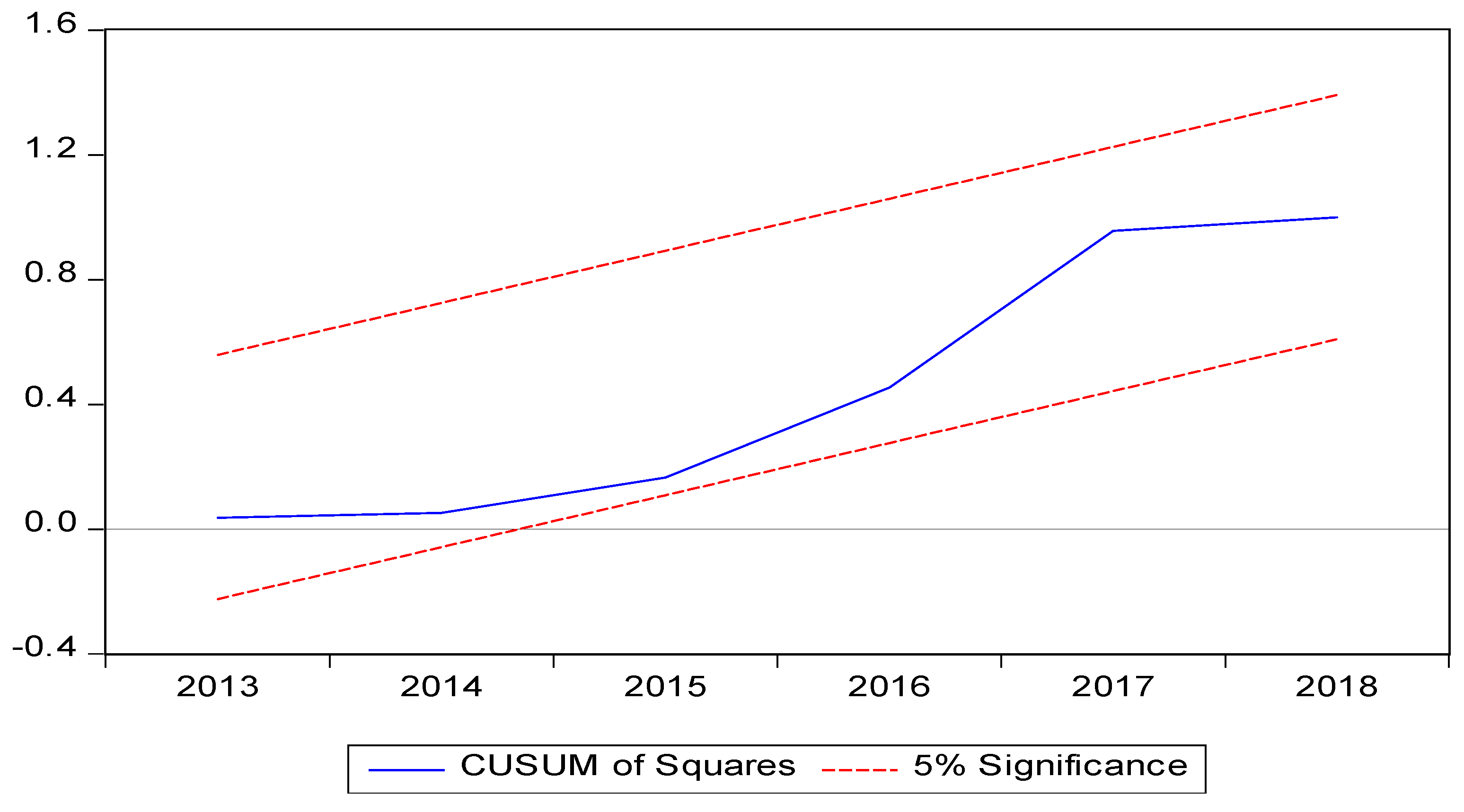
Table 5.6 above reports the results of several tests conducted for the reliability and robustness of the model. Based on the statistics reflected by the table, the analysis does not have the problem of serial correlation among residuals, as the value of the Breusch-Godfrey LM statistic is insignificant at a level of 5%. Likewise, the nominal test value of the Breusch-Pagan-Godfrey test also rejects the hypothesis of having heteroscedasticity among the residuals. Additionally, the p-value greater than 0.05 for the Jaque-Bera test results supports the claim of normality in the datasets. Finally, the Ramsey RESET test statistic implies that the model is correctly specified. This is because the significance value of the test is above the 5% significance level, which suggests a correctly specified functional form. When dealing with time-series data, one should employ a correctly specified model; otherwise, the results might become biased and will not be reliable enough to consider for decision-making (Hansen, 1992; Farhani & Ozturk, 2015). The study employed CUSUM and CUSUMSQ tests to look for the stability of the model. The tests check the systematic variability of the coefficients and check if a process is drifting away from its mean. The results for these particular methods in Figures (4.2) and (4.3) suggest that the model is stable in both the long and short run; this is because the blue trend line does not cross the red one at a 5% level of significance in both of the tests mentioned above.
Figure 5.
1 CUSUM Test.
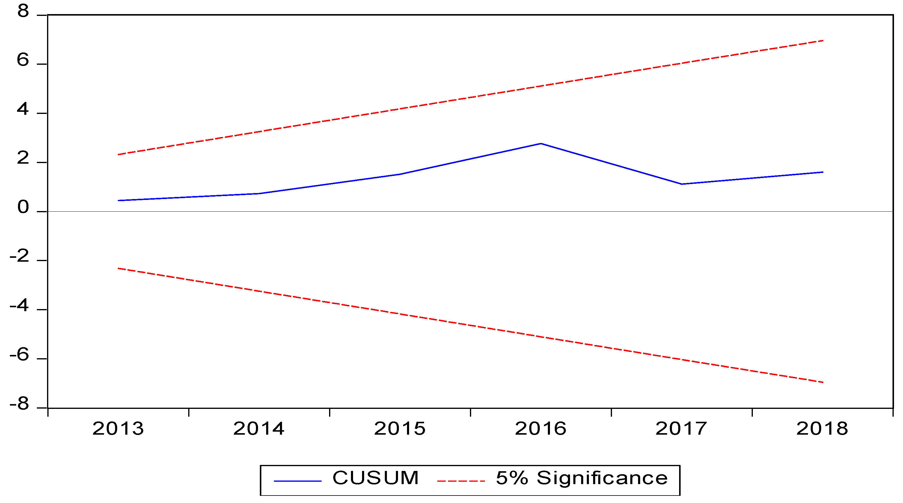
Figure 5.
2 CUSUM of Square Test.
6. Conclusion and Policy Implications
Malaysia faces challenges related to CO2 emissions and wealth inequality, much like many other industrialized and developing countries. Although much research has been done on the relationship between these two factors in different nations, much has not been done, particularly in Malaysia. In order to close this gap, the current study looks into how income inequality and several other factors affected Malaysia’s CO2 emissions between 1989 and 2023.
The unit root test and the ARDL limits testing approach were used in the study to investigate stationarity and the short- and long-term correlations between income inequality, CO2 emissions, and other contributing factors. In order to explore the existence of the Environmental Kuznets Curve (EKC), which postulates an inverted U-shaped relationship between income levels and CO2 emissions, the study also included the squared term of GDP per capita. The unit root test results showed that all other series are stationary at the initial difference, except for energy consumption, which is stationary at the level. Because of the I(0) and I(1) series, co-integration analysis could be conducted using the ARDL model. A co-integrated, strong, and substantial long-run link between CO2 emissions, GDP per capita, GDP per capita squared, Gini coefficient, population, urbanization, energy consumption, industrialization, and trade openness was found using the ARDL approach. These results confirm the presence of Malaysia’s Environmental Kuznets Curve (EKC), or the inverted U-shaped relationship between income levels and CO2 emissions, suggesting that early economic expansion development stages initially have a detrimental influence on environmental quality. However, when people prioritize eco-friendly habits and stricter environmental restrictions, the quality of the environment starts to improve after a certain point in growth.
Additionally, the study found a strong correlation between Malaysia’s CO2 emissions and income disparity, suggesting that income inequality had a favorable impact on CO2 emissions. This implies that disparities in income worsen the state of the environment since the wealthier groups tend to consume more products and services that pollute the environment, which in turn encourages the use of non-renewable energy sources for industrial activity. All factors considered in the study considerably impacted Malaysia’s CO2 emissions over the given period.
Any policy intended to bring economic growth to Malaysia needs to consider the role of income inequality in its planning so that it can increase sustainability and reduce CO2 emissions. For further studies, one can consider the role of poverty, agriculture, and financial development. Besides, one can also add the square of Gini to observe nonlinear connections and the interaction term of GDP per capita and Gini coefficient to test if the impact of income inequality on CO2 was subjected to income levels.
References
- Ali, A. , Bibi, S., & Shahbaz, M. Testing environmental Kuznets curve hypothesis in Pakistan. Environmental Science and Pollution Research, 2017, 24, 25245–25254. [Google Scholar]
- Ali, H. , Yousaf, S. U., & Jamil, F. The impact of renewable energy consumption on economic growth and environmental quality: Evidence from South Asian economies. Energy Reports, 2020, 6, 623–633. [Google Scholar]
- Aslam, B. , Wang, X., & Zhang, Y. Climate change and groundwater resources: A case study approach. Water Resources Management, 2021, 35, 1032–1046. [Google Scholar]
- Baek, J. , & Gweisah, G. Does economic growth influence CO₂ emissions in Nigeria? Renewable and Sustainable Energy Reviews, 2013, 18, 119–125. [Google Scholar]
- Baloch, M. A. , Danish, B., & Ozturk, I. Investigating the role of energy consumption and economic growth on environmental quality: Evidence from panel data analysis. Renewable and Sustainable Energy Reviews, 2020, 129, 109901. [Google Scholar]
- Barbier, E. B. Poverty, development, and environment. Environment and Development Economics, 2010, 15, 635–660. [Google Scholar] [CrossRef]
- Basri, N. E. A. , Ismail, S. N. S., & Hanafiah, M. M. Sustainable water management in developing countries. Environmental Science and Pollution Research, 2015, 22, 5120–5130. [Google Scholar]
- Begum, R. A. , Sohag, K., Abdullah, S. M. S., & Jaafar, M. CO₂ emissions, energy consumption, economic and population growth in Malaysia. Renewable and Sustainable Energy Reviews, 2015, 41, 594–601. [Google Scholar]
- Bhattacharya, S. The economic impact of climate change on developing nations. Journal of Environmental Economics, 2019, 12, 87–102. [Google Scholar]
- Cho, R. (2018). The effects of climate change on water resources. Columbia Climate School News.
- Dinda, S. Environmental Kuznets curve hypothesis: A survey. Ecological Economics, 2004, 49, 431–455. [Google Scholar] [CrossRef]
- Dogan, E. , & Turkekul, B. CO₂ emissions, real output, energy consumption, trade, urbanization, and financial development: Testing the EKC hypothesis for the USA. Environmental Science and Pollution Research, 2015, 22, 10724–10734. [Google Scholar]
- Gill, A. , Hasan, A., & Khan, A. Water scarcity and climate change: A case study of South Asia. International Journal of Water Resources, 2018, 12, 112–125. [Google Scholar]
- Hailemariam, A. , Dzhumashev, R., & Shahbaz, M. The impact of climate change on economic growth: Empirical evidence from cross-country panel data. Environmental Economics and Policy Studies, 2019, 21, 775–810. [Google Scholar]
- Hassan, S. A. , Mahmood, H., & Ghaffar, R. Renewable energy consumption and environmental degradation: The role of economic growth and financial development. Environmental Science and Pollution Research, 2019, 26, 22515–22525. [Google Scholar]
- Hübler, M. The economics of climate change mitigation. Journal of Environmental Economics and Policy, 2017, 6, 321–341. [Google Scholar]
- Jorgenson, A. K. , Schor, J. B., & Huang, X. Income inequality and carbon emissions in the United States: A state-level analysis, 1997–2012. Ecological Economics, 2016, 134, 40–48. [Google Scholar]
- Khalid, U. , & Yang, M. Climate change, agriculture, and food security: Evidence from Asia. Agricultural Economics, 2021, 52, 451–469. [Google Scholar]
- Knight, K. W. , Rosa, E. A., & Schor, J. B. Could working less reduce pressures on the environment? A cross-national panel analysis of OECD countries, 1970–2007. Global Environmental Change, 2017, 47, 67–75. [Google Scholar]
- Koswanage, N. Deforestation and water scarcity: The Asian dilemma. Nature Sustainability, 2015, 2, 39–46. [Google Scholar]
- Magnani, E. The environmental Kuznets curve, environmental protection policy, and income distribution. Ecological Economics, 2000, 32, 431–443. [Google Scholar] [CrossRef]
- McGee, J. A. , & Greiner, P. T. Environmental justice and climate change adaptation. Sociological Perspectives, 2018, 61, 805–825. [Google Scholar]
- Mehraaein, M. , Rostami, A., & Davari, S. Groundwater management and climate change: A case study of Iran. Water Policy, 2021, 23, 1098–1115. [Google Scholar]
- Mittmann, J. L. , & de Mattos, R. S. The role of economic policies in climate change adaptation. Energy Policy, 2020, 140, 111457. [Google Scholar]
- Munasinghe, M. Is environmental degradation a major threat to sustainable economic growth? Environment and Development Economics, 1999, 4, 451–474. [Google Scholar]
- Murad, M. W. , & Mustapha, K. M. Sustainable development and water resources management in Southeast Asia. Journal of Environmental Management, 2010, 91, 940–948. [Google Scholar]
- Narayan, P. K. , & Narayan, S. Carbon dioxide emissions and economic growth: Panel data evidence from developing countries. Energy Policy, 2010, 38, 661–666. [Google Scholar]
- Nurgazina, Z. , Zhakupova, S., & Baimukhamedova, A. Climate change and agricultural adaptation: The case of Central Asia. Environmental Policy and Governance, 2021, 31, 148–165. [Google Scholar]
- Rai, A. Climate change adaptation strategies: Lessons from South Asia. International Journal of Climate Change Strategies and Management, 2019, 11, 24–39. [Google Scholar]
- Shahbaz, M. , Lean, H. H., & Shabbir, M. Environmental Kuznets curve hypothesis in Pakistan: Cointegration and causality analysis. Renewable and Sustainable Energy Reviews, 2016, 54, 1423–1431. [Google Scholar]
- Siwar, C. , & Murad, M. W. Sustainable development and water resources management in Malaysia. International Journal of Water Resources Development, 2001, 17, 469–480. [Google Scholar]
- Torras, M. , & Boyce, J. K. Income, inequality, and pollution: A reassessment of the environmental Kuznets curve. Ecological Economics, 1998, 25, 147–160. [Google Scholar]
- Wang, X. , Liu, J., & Zhang, Y. Groundwater depletion and climate change: A global perspective. Water Resources Research, 2020, 56, e2019WR026467. [Google Scholar]
- World Health Organization (WHO). (2015). Global water quality and human health. WHO.
- Wolde-Rafael, K. , & Idowu, A. Climate change, poverty, and sustainable development in Africa. Journal of Sustainable Development in Africa, 2017, 19, 124–138. [Google Scholar]
- Yang, H. , Zhang, J., & Wang, Z. The impact of climate change on freshwater resources. Environmental Research, 2020, 187, 109563. [Google Scholar]
Disclaimer/Publisher’s Note: The statements, opinions and data contained in all publications are solely those of the individual author(s) and contributor(s) and not of MDPI and/or the editor(s). MDPI and/or the editor(s) disclaim responsibility for any injury to people or property resulting from any ideas, methods, instructions or products referred to in the content. |
© 2025 by the authors. Licensee MDPI, Basel, Switzerland. This article is an open access article distributed under the terms and conditions of the Creative Commons Attribution (CC BY) license (http://creativecommons.org/licenses/by/4.0/).
Copyright: This open access article is published under a Creative Commons CC BY 4.0 license, which permit the free download, distribution, and reuse, provided that the author and preprint are cited in any reuse.


