
Submitted:
11 April 2025
Posted:
14 April 2025
You are already at the latest version
Abstract
Corrosion in combination to fatigue cycling loading is inevitable and becomes a challenging problem even though selection of inherently corrosion protected materials has been applied based on established in house experience. Aero engine mount structures are exposed to dust and salt environmental conditions both during operational and non-operational periods. Predictions of remaining useful corrosion fatigue life are becoming tough due to the materials strength degradation5 from the service condition and hence rationalized approach is being currently used to assess their structural integrity. This paper brings a novel approach to predict the corrosion fatigue by proposing random parameter model in combination to experimental data. The two random parameter model with probability method is employed here to determine the time-independent corrosion fatigue life of magnesium structural casting used heavily in mount structures. The same is also correlated with experiments data from literature for validating the proposed stochastic corrosion fatigue model to address the technical variance occurred during in service.
Keywords:
Corrosion
; fatigue
; magnesium casting
; fatigue damage accumulation
; oxidation
; pitting
1. Introduction
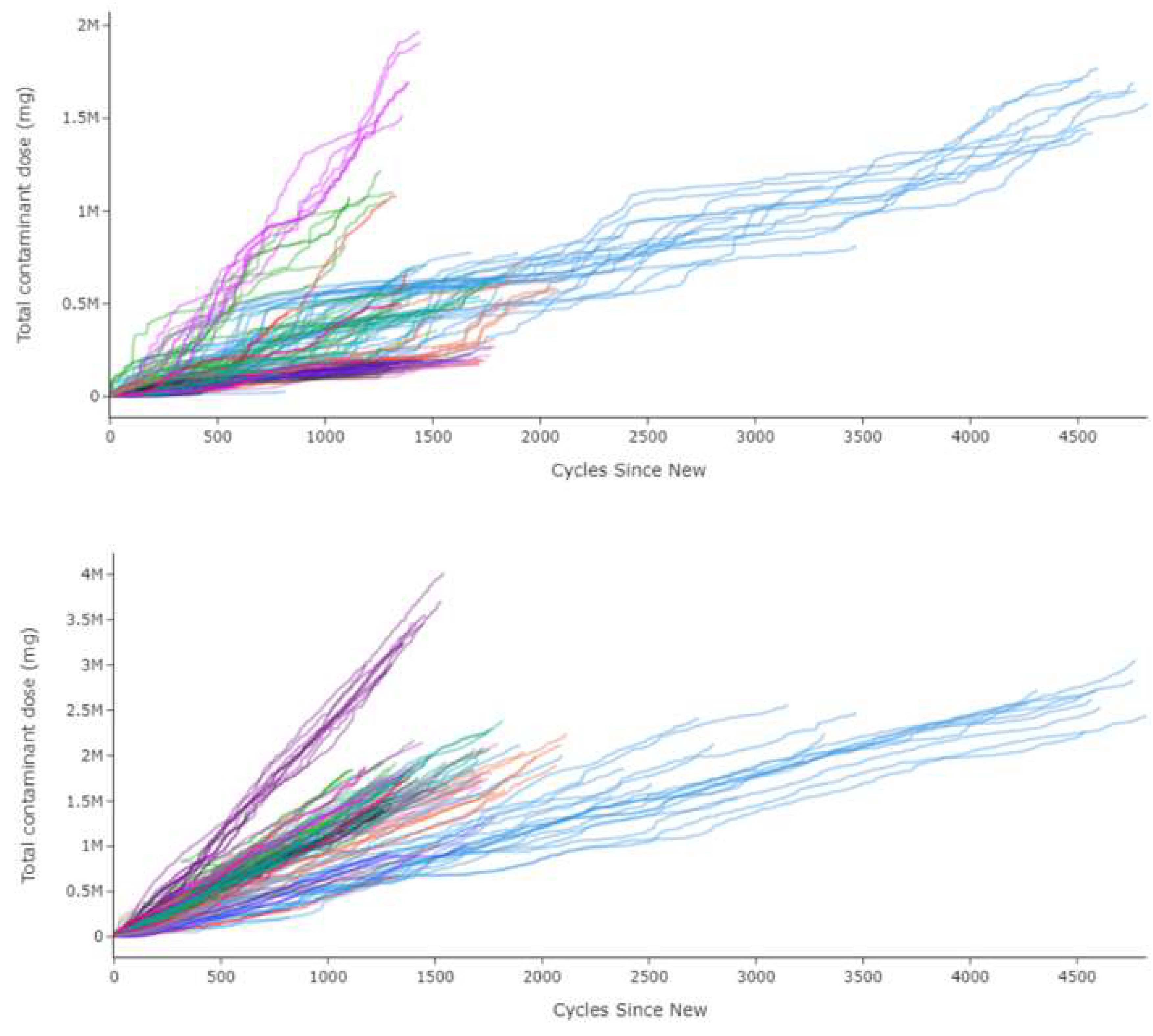
The magnesium cast alloys are potential candidate materials for the applications in automobile and aerospace industries due to their abundance availability and at low cost. However, in real service conditions, the structural components often suffer from the corrosive attach due to their exposure to aggressive environment in along with aggravated aging condition of magnesium structural casting. There are many previous studies on this magnesium cast alloys and their fatigue corrosion strength that are available as plenty [1, 8]. But the available accurate model that predicts the fatigue life of corrosive environment on magnesium alloy is still limited. In aerospace industry particularly static components in aero engine that are being manufactured by magnesium cast alloys are sometimes evaluated conservatively to maintain their airworthiness during their services conditions. In particular to structural magnesium casting alloy which is prone to corrosive attach along with operational fatigue loads. Building up a corrosion fatigue model for on-wing condition of aircraft engine structural components is crucial but in necessary demand as it helps to optimizes the fleet planning in effective way. Additionally, it could also be reducing the engine maintenance and consequently decreases costs. Most of the environmental contaminants are of from salt, sand, dust, SO2, and SO4 for every flight from Jan 2012 to December 2020 with the worth damage due to lack of corrosion fatigue model with incurred loss of approximately 7.5million pounds. With data quenching through internal flight data sets for contaminations model with the actual flight cycles, the salt environmental condition is the worst in deteriorating the structural integrity of engine static components, compared with the other conditions on corrosion fatigue failure mode. The severity of salt environmental exposure for Rolls Royce engines with various operators can be observed in the figure 1 compared dusted condition (different color lines indicates different airlines).
Figure 1.
Amount of total contamination by dust and salt exposure of aero engines over cycles for different airline operators for past eight year.
Figure 1.
Amount of total contamination by dust and salt exposure of aero engines over cycles for different airline operators for past eight year.
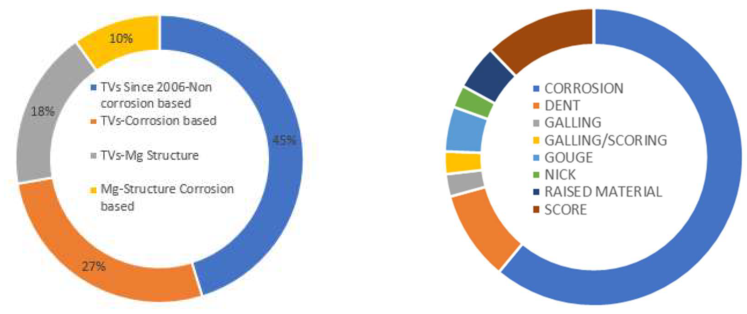
There are also numerous requests for addressing the technical variances during regular maintenance visit of the aero engine to magnesium structural casting based engine mounting structures at often. Out of all these technical variances collected for last decades, 27% of which are based on corrosion attacking on structural integrity for one particular engine program. Out of this, 18% are based on corrosion fatigue issues with the magnesium structural casting for an intermediate structure.
Figure 2.
Technical variances of corrosion problems and related magnesium casting support structure.
Figure 2.
Technical variances of corrosion problems and related magnesium casting support structure.
2. Corrosion Fatigue Model
The available conventional corrosive fatigue model for assessing the corrosion fatigue failures on magnesium mount structural casting is not quite accurate as the formation of corrosion pit is random nature and the empirical equations that are derived out from specimen samples are majorly in linear format. Generally, casting shrinkage and porosity in as cast magnesium alloys can specially act as stress concentration sites for fatigue crack initiation additional to the oxide inclusions that are prompted under corrosive environmental conditions. These preferential sites for fatigue crack initiation will be related to formation of pits on the surface and at particular to tensile fiber stress locations. When magnesium mount structural casting is exposed to corrosive environment, both anodic and cathodic reactions are happening with a result of releasing hydrogen gas that plays major role in environmental assisted cracking [1-3].
Magnesium dissolution in aqueous solution is an anodic reaction whilst the hydrogen evolution is a cathodic reaction. Hydrogen could diffuse into magnesium matrix through corrosion pits formation and then cause the hydrogen embrittlement that could significantly reduce the mechanical strength of magnesium alloys. Thus, although the size of the pits is smaller than that of oxide inclusions on fracture surfaces fatigue cracks can still preferentially nucleate at pits even at lower stress amplitude in NaCl solution than at air.
2.1. Fatigue life of Magnesium Structural Casting Model for Corrosion
The difference of fatigue life of magnesium structural casting material with and without corrosive environmental condition has been assessed from available literatures to create a material data base for the assessment of the filed technical variances in along with available internal source.
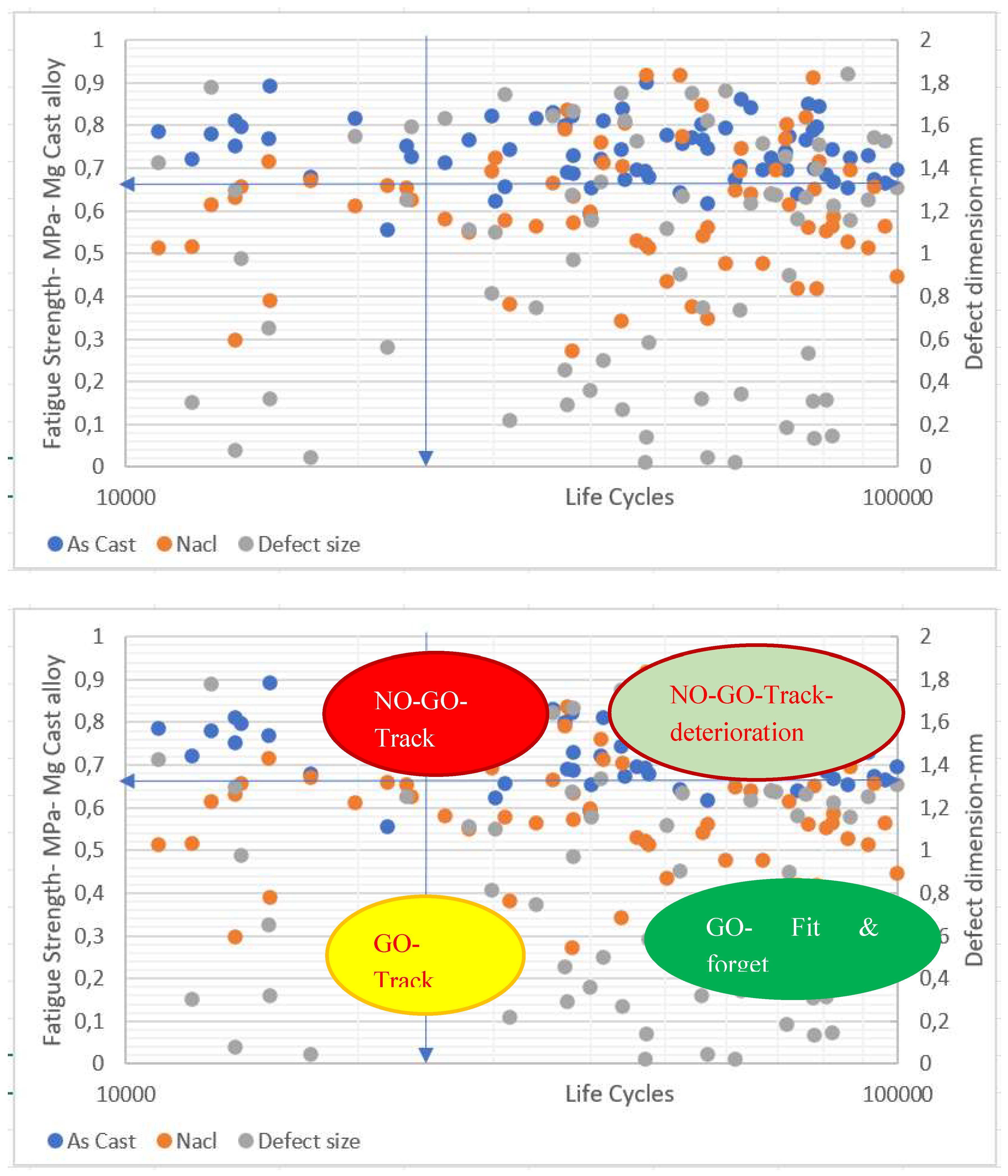
The fatigue life of the as cast and NaCl solution exposed to magnesium structure is shown in figure 3 from reference 1 along with the defect sizes which varies from minimum 0.18mm to maximum 7.4mm of equivalent spherical diameter. Figure 3 also carries internal Rolls Royce material data for magnesium cast structure without any corrosion defects (as cast condition) which coincides into higher fatigue life cases . This fatigue strength over corrosion environmental condition generally can also be degraded over time which is not considered here for simplification purpose.
The empirical relationship of corrosion fatigue life of magnesium structural casting could be obtained from this available experimental data. These fatigue data is for finite corrosion pit data and has some limitations on applying directly in to solving field corrosion pit issue for magnesium structural casting. There is a need for an efficient model that address random nature of fatigue, corrosion (pit) and load scenarios. Otherwise industry is left only with rational approach which is inefficient sometimes. The following section proposes stochasitic corrosion fatigue model with simplified way.
2.2. Stochastic Process and Random Variables- Formulation
In order to explain quantitatively and investigate the regularities of the random phenomenon, it is a common practice to introduce a mathematical formulation that brings the randomness together with an appropriate measure of the possibilities of occurrences of various uncertain outcome of an experiment. Such a model forms a basic system for probability model in which main notions are defined as:
Sample space: This is defined as the collection of all possible outcomes from the experiments.
Random event: Event that can happen at unpredictable way.
Probability: Probability of the event.
A sample space will be denoted as Ω which contains all the possible or elementary outcomes of an observation denoted as γ, which satisfies, γ∈Ω. Let ξ be denoted as the family of subsets of Ω, described as the family of random events with which a probability of event P is defined. The probability of event P is described here as the probability of reaching required fatigue life at critical porosity fraction. The probability of event P is a function whose arguments are random events which is element of ξ so that it follows the following three axioms of modern probability [2],
0≤ P(A) ≤ 1, for each A∈ ξ,
P(Ω) = 1
For any countable collection of mutually disjoint events, A1, A2, …An in ξ:
P{ ∪ An} = Σ P(An)
It is clear that in experiments on random phenomena, various outcomes or elementary events can occur. In many situations, they are represented by the real number X (γ). It is also possible that a real number can be assigned to each elementary event, γ∈Ω. X(γ) is called as a random variable which is defined as a real-valued function X = X(γ), γ∈Ω, defined on the sample space Ω, such that for every real number ‘x’ then the probability is defined as,
P{Ω: X(γ) ≤ x }
The existence of the probability of event {γ: X (γ) ≤ x} ensures that the probability of any finite or countable infinite combination of such events is well defined as P {x1 < X (γ) ≤ x2}.
The probabilistic behaviour of a random variable X (γ) is completely and uniquely specified by cumulative distribution function FX (x) which is defined as,
FX (x) = P {X (γ) ≤ x}
By definition, the distribution function always exists and is a non-negative and non-decreasing function of the real variable ‘x’.
Property 1:
From the properties cumulative distribution function, it follows that,
FX (-∞)
= 0 ; and FX (+∞) = 1
(2)
Property 2 For any two real numbers a, b such that a < b, the probability is computed as,
P {a < X ≤ b) = FX (b) – FX (a).
Property 3 The function fX (x) is non-negative. Since integrating the density function on an event gives us the probability of the event. This property can be proved easily since the probability density function is the derivative of the cumulative distribution function. This cumulative function being a non-decreasing function, its derivative can never be negative.
2.2.1. Single Random Variables –Formulations.
The basic probability model for a single random variable is defined in this section.
By assuming, a random variable X (γ) is termed as a continuous random variable if its probability distribution function FX (x) has a density function, such that,
Where ‘U’ is defined as any dummy variable. The function fX (x) is called the probability density function of the random variable X (γ). Hence,
Further properties of probability density function are,
Physically when the random samples are drawn from the sample spaceΩ, it is essential to compute the mean and standard deviation of these random samples so that the probability density function could be derived out based on the type of distribution function it follows. When the random samples are repeated ‘N’ times, by having the X as random variables, x as real set numbers, among N experiments, the real value xi can be repeated as ni times, the average or mean is calculated as
Intuitively, the quantity of is none other than measuring the probability of obtaining the result xi over N experiments. Then the equation 9 can be re-written as,
When N as random samples which are infinitely growing, and X is the random variable which sometimes equal to the real number xi, the ratio goes to an infinitesimally small quantity which represents fx(xi). dx at point xi. The mean or average value of a random variable is defined as an operator called expectation operator, E(X).
The notation E (.) stands for the average value operator, commonly called s mathematical expectation. The equation 11 is a similitude of centre of gravity equation which is defined as a summation of the product of each area strip to the length of the strips divided by total area of the body. The denominator of the equation 11 is representing the total area of the probability density function which is unity. Hence the equation 11 becomes,
Equation 12 is also called as average or mean value of the random variables X (γ) which is denoted as μX.
The variance of random variables X(γ) is defined as,
The square root of the equation 13 is called as the standard deviation of the random variables.
The ratio of variance to mean provides a coefficient of variation which normalizes the spread of occurrence of real numbers from the random variables X(γ).
Ideally, the equation 15 represents the standard deviation of random variables which is containing difference of mean square value to the square of the mean of random variables. Physically, σX measures the dispersion of the experiments results around its average value. When σX is small, the probability density function of X is a curve concentrated around its mean. When σX is large, this curve flattens and gets wider.
By the same means, it can be introduced the moments of any order n:
and the order ‘n’ centered moments is formulated by,
The characteristic function is an important analytical tool which enables to analyse the sum of independent random variables. Moreover, this function contains all the necessary information specific to the random variables X.
3.2.2. Bivariate and Multivariate Random Variables –Formulations.
The basic probability model when there are two or more random variables is defined in this section by above description which is based on a single random variable. This means it is also possible to generalize the above equations for the multi-dimensional case. It is focused now instead of random variables, to random vectors.
Let be X a two dimensional random vector X = (X1, X2). The joint cumulative distribution function of the random variables X1 and X2 are also called the cumulative distribution function of the random vector X which is defined as similar to equations 1 and 4.
FX1, X2 (x1, x2) = P {x1 ≤ X (γ) ≤ x2}
Directly from the probability of axioms defined for single random variables alternatively changed as:
0≤ P {x1 ≤ X (γ) ≤ x2} ≤ 1, for each A∈ ξ,
P(Ω) = 1, or FX1, X2 (+∞, +∞) = 1,
FX1, X2 (x1, -∞) = 0 and FX1, X2 ( -∞, x2) =0,
For any countable collection of mutually disjoint events, A1, A2, …An in ξ:
P{ ∪ An} = Σ P(An)
As with the case of a single random variable, in the vector case, it is necessary to build a function called the joint probability density function of the variables X1 and X2 such that, the integration of these two events in the sample space, the conditional probability is obtained as:
This also allows, to
It is now essential to bring the basic fundamental properties of conditional probability of events, that gives,
The condition for the equation 22 is at X1 and X2 is independent random variables, and then the joint probability density function of two independent random variables is given by the product of their respective marginal densities.
Similarly, the mean, variance, moments and centered order of moments are also defined for bi-variate random variables.
Joints moments of order n and m for X1 and X2 random variables,
The centered ordered n, m moments,
Among the centered moments the most important parameter, is called covariance between the two random variables X1 and X2.
The matrix
The equation 27 is called variance-covariance matrix of (X1, X2) vector. If these two random variables are independent to each other, then their covariance is zero. If their correlation value is zero, then these variables said to be at orthogonal.
The correlation coefficient between the two random variables X1, and X2 is calculated as,
For transformation of n-dimensional random vectors, Jacobian of coordinates mapping is used. The stochastic equation which may be used to describe the time dependent corrosion process should consist of two main parameters that describe fluctuation in environmental conditions, and microscopical structural behavior of the material. A correlation of microscopic mechanisms of corrosion with its macroscopic statistical nature is needed for this development of stochastic corrosion fatigue equation. The macroscopic mechanisms of corrosion of material can be derived as referencing empirical equation from experiments. Microscopical structural behavior of material can be contributed with two factors: consideration of fluctuation in environmental, and average background of structure superimposed by inhomogeneous fluctuations due to variety of inherent defects.
The stochastic equation which may be used to describe the process of corrosion as presented above stochastic process with random variable as pit formation with respect to time, fatigue life and stress (loading). Because fluctuations of the environment or of the microscopic structure led to stochastic fluctuations of the corrosion rate, the corrosion rate should obey the above-mentioned stochastic corrosion fatigue model in along with experimentally obtained empirical equations (as presented in next section).
2.3. Stochastic Corrosion Fatigue (SCF) Model
Let the stress amplitude (Sa) has cumulative density function (CDF) of FSa, then lifetimes size of corrosion pits (N*CP) has got CDF of FNCP and the relationship between these two CDF is established for NaCl as:
The probability distribution function is derived out from the above equation by,
The mean and variance have also been formulated for each dependent and independent random variable.
Now with the available probabilistic parameters, based on Monte Carlo random model technique the range of experimental parameters are sampled for 1000 times as it is shown in figure 4.
Figure 4.
Stress-Life curve for as cast versus NaCl exposed Mg cast alloy from Random model with experimental raw data (#1000 random samples).
Figure 4.
Stress-Life curve for as cast versus NaCl exposed Mg cast alloy from Random model with experimental raw data (#1000 random samples).

3. Implementation of SCF Model to Technical Variances
If the grain boundary near to the free surface is not very well protected by an oxide layer, oxygen gas or other embrittling species may diffuse along the boundary and react with grain boundary precipitates. Under this influential condition of loads, stress spikes at the cavities are present around the grain boundary precipitates which are accelerated by repeated environmental exposure of the structures during their services.
Combination of surface diffusion and slip step oxidation promotes enhanced kinematic irreversibility of cyclic slip that causes earlier fatigue cracks to nucleate in the absence of other mechanisms. This step is also accelerated by porosities and voids in magnesioum structural casting.
Preferential oxidation at certain micro structural sites such as at the intersection of a grain boundary with a free surface, causes microscopic stress concentrations (notches) to develop. The micro notches elevate the local stresses and promote crack nucleation. The expected high stress profile features are also identified for this intercase structures and based on filed experiences, the identified stress corrosion features are assessed for their corrosion fatigue life to avoid any premature failures.
The fleet reported corrosion fatigue defects and corresponding fatigue life to be cleared for the required life mission, and at experienced fatigue loading conditions, the reported technical variances are assessed based on the proposed stochastic fatigue model for corrosion (SFC) as it is showed in figure 5 instead of any qualtative based assessment which has quite conventional method usually been followed.
Commonly, these technical variance of corrosion issues on magnesium stuctural casting is being carried out based on individual assessment with rational qualitative basis. This proposed SCF model will bring not only a new concept with quantitative approach but also the remaining useful life period is effectively calcualted with more effective way based on the evidence collected with experimental data.
Figure 5 gives the real flying fleet corrosive data within the specification of randomly generated fatigue life of known corrosive defects that has been calculated with proposed stochastic corrosive fatigue model with a normalised stress plot of the engine support structure. Since it has been cleared for the required number of flight cycles, the real flying corrosion attacked components are at constant life curve but with various bubble sizes that indicate the corrosion sizes with varying fatigue strength.
The following results are obtained from the presented stochastic corrosion fatigue model with actual fleet data of aeroengine of front flanges raised for technical variances.
4. Conclusions
Corrosion from real filed and in service issues on magnesium structural casting of engine mount critical structure is being analyzed and assessed based available and qualitative assessment methods which put many rejections on the part despite it could have more useful life period. This is challenged and addressed by proposing a real time automated data analysis system that is proposed based on stochastic corrosion fatigue model. This model is developed and validated with based on corrosion related fatigue data from literature as well as from in house material data sets. This paper brings not only a novel approach to predict the corrosion fatigue by proposing random parameter model in combination to experimental data but also effectively solve the two random parameters model with probability method to determine the time-independent corrosion fatigue life of magnesium structural casting used heavily in mount structures. The same is also correlated with experiments data from literatures for validating the proposed stochastic corrosion fatigue model to address the technical variance occurred during in service.
Supplementary Materials
Since it involves company proprietary technical data, it could be available based in individual queries to the corresponding authors.
Author Contributions
Govindarajan Narayanan- GN, Andrej Golowin -AG: “Conceptualization, GN.; methodology, GN.; software, GN.; validation, GN., AG.; formal analysis, GN; investigation, GN.; resources, GN, AG; data curation, GN.; writing—original draft preparation, GN.; writing—review and editing, AG, GN.; visualization, GN.; supervision, AG.; project administration, GN.;
Funding
This research received no external funding.
Data Availability Statement
Since it involves company proprietary technical data, it could be available based in individual queries to the corresponding authors.
Acknowledgments
Acknowledgement is fully given to RRD, Brandenburg.
Conflicts of Interest
Declare conflicts of interest or state “The authors declare no conflicts of interest.” Authors must identify and declare any personal circumstances or interest that may be perceived as inappropriately influencing the representation or interpretation of reported research results. Any role of the funders in the design of the study; in the collection, analyses or interpretation of data; in the writing of the manuscript; or in the decision to publish the results must be declared in this section. If there is no role, please state “The funders had no role in the design of the study; in the collection, analyses, or interpretation of data; in the writing of the manuscript; or in the decision to publish the results”.
Appendix A
Analytical Model development:
Pit growths accelerate during flight loads, to model this, a volumetric rate of material degradation (either pit formation or pit growth or both) is a volume reduction over period of flying, post exposure of front engine mount at nonflying condition (parked engine).
Volumetric change (rate) over time can be expressed by Faradys law from electrolysis, and mass density. M, molecular weight of magnesium (kg/Mol), n, valance electron of magnesium to get react during incubation period, Ip, pitting current (C/s) which can be calculated as per Arrhenius relation (reaction rates with temperature dependant with Enthalpy, J/Mol and universal gas constant R, J/Mol.K, and temperature in Kelvin), and mass density.
Where, for magnesium alloy, enthalpy value is assumed to be 60 kJ/Mol.
With assumption of half spherical shape of pit formation with aspect ratio of φ, b major axis radi and a is minor axis radi, hence the volume is given by,
By combing above equations, to find out the pit radi, including electrolysis process on corrosion event, Ishira’s model [7] that combines stress (Sa) and corrosion fatigue cycles (N) into empirical equations as below:
Integrating over time, final pit size can be calculated,
From this life can also be estimated when corrosion pit size and working stress are known,
This model closely corelated with the randomly generated corrosion pits data from technical variance data base of front engine mount structure flange in aligning to the empirical models from experiments and hence validated to apply for any technical deviations within these operating conditions (Figure 5- orange-coloured points- Corrosion Pit Model).
References
- Wang S. D., Xu D. K., Wang B.J., Han E. H., and Dong C.: "Effect of corrosion attack on the fatigue behaviour of an as- cast Mg-7%Gd-5%Y-1%Nd-0.5%Zr alloy", Materials and Design, 2015.
- Narayanan G.: “Probabilistic fatigue model for cast alloys of aero engine applications”, International Journal for Structural Integrity, 2020.
- Haiyun. H.: “Stochastic theory of fatigue corrosion”, Physics Letters A 261, 1999.
- Urbano.J, Golowin. A, Löhnert. S, and Bestle. D.: “Mechanical Integrity of Steel Discs with Corrosion Pits”, MATEC Web of Conferences 165, Fatigue 2018, 2018.
- Larrosa. N, and Akid. R. : “ Corrosion Fatigue- A review of damage tolerance models”, International Materials Reviews, 2017.
- Mao. M, Zhang. X, Tu. S, and Xuan. F. : “ Prediction of crack initiation life due to corrosion pits”, Journal of Aircraft, 2014.
- Ishihara S, Saka S, Nan ZY. : “Prediction of corrrosion fatigue lives of aluminium alloy on the basis of corrosion pit growth law”. Fatigue Fract Eng Mater Struct. 2006.
Figure 3.
Stress-Life curve for as cast versus NaCl exposed Mg cast alloy [1].
Figure 3.
Stress-Life curve for as cast versus NaCl exposed Mg cast alloy [1].
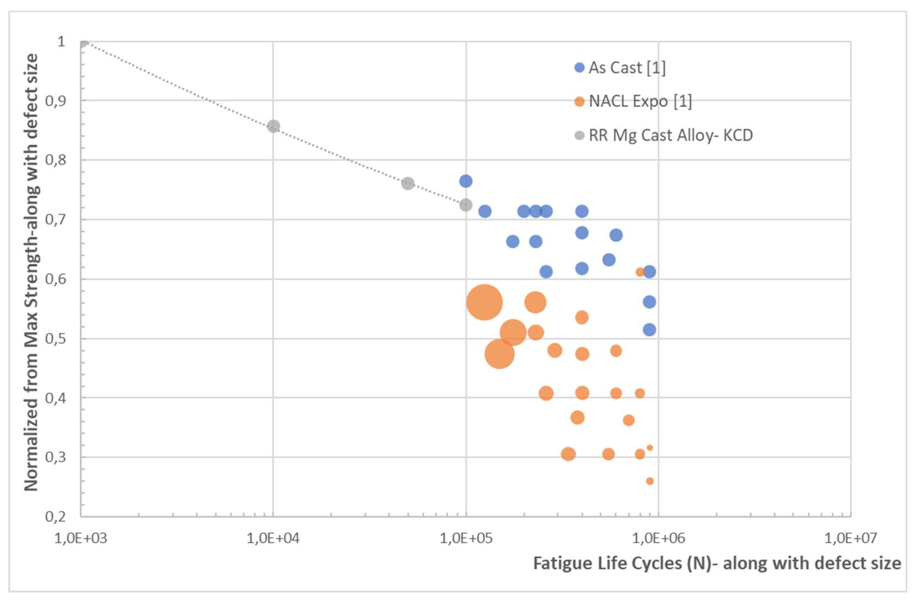
Figure 5.
Fleet technical variance of corrosive fatigue loading condition of engine intermediate Magnesium cast structure along with SFC model.
Figure 5.
Fleet technical variance of corrosive fatigue loading condition of engine intermediate Magnesium cast structure along with SFC model.
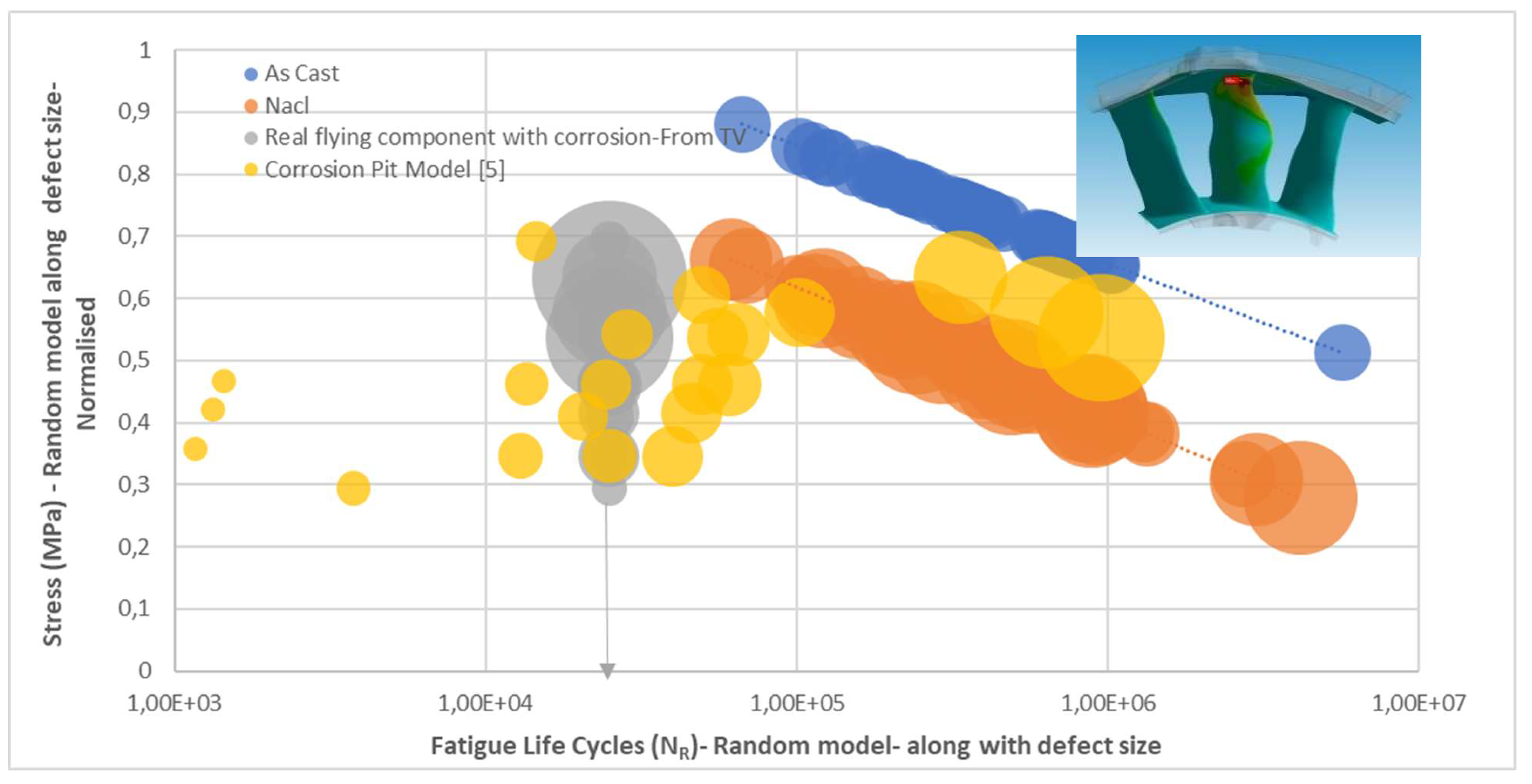
Figure 6.
Real data set for Mg corrosion pit formation from fleet data of engine intermediate Magnesium cast structure along with SFC model.
Figure 6.
Real data set for Mg corrosion pit formation from fleet data of engine intermediate Magnesium cast structure along with SFC model.
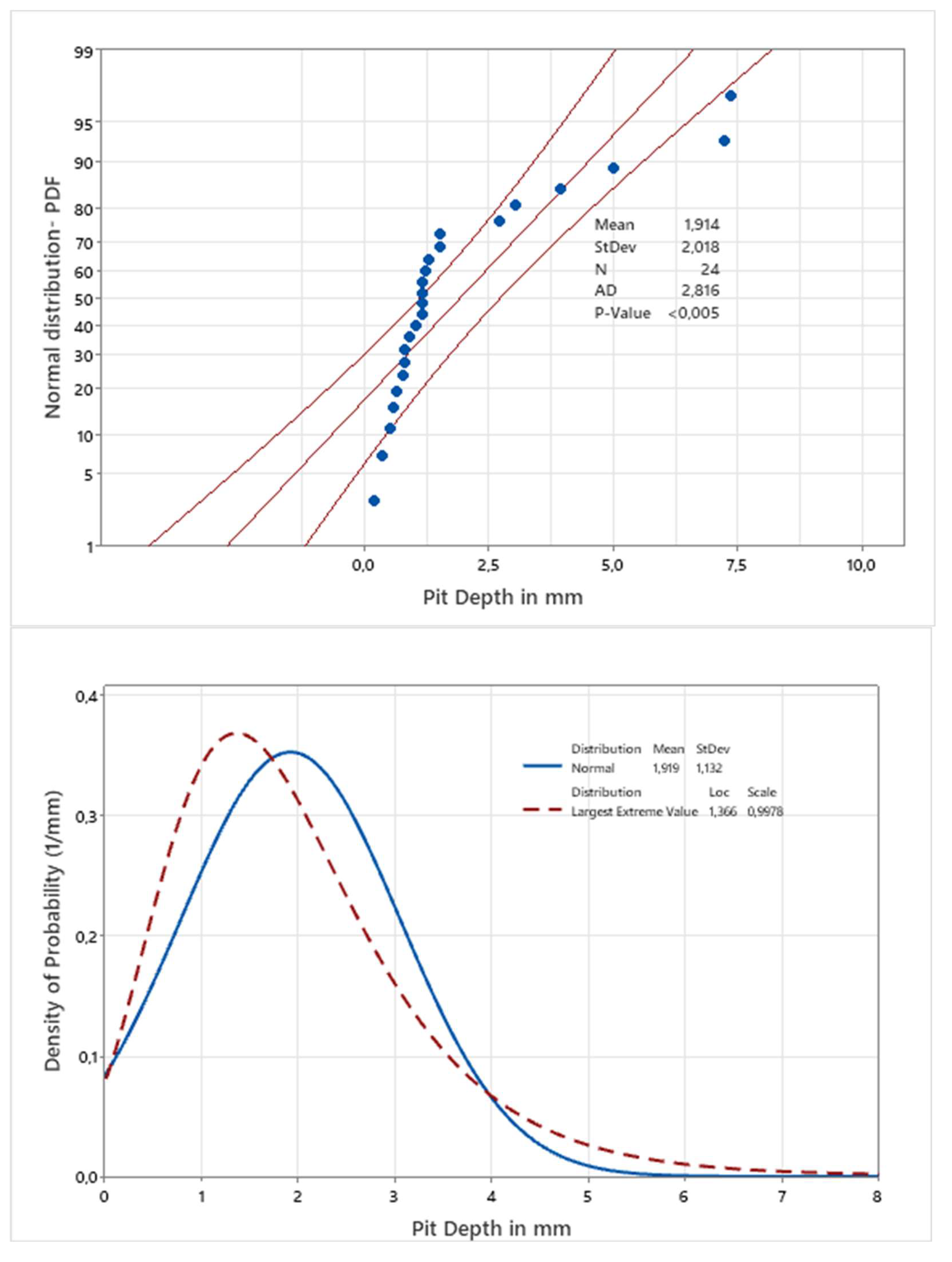
Figure 7.
Stochastic corrosion fatigue model assessment on fleet technical variance based on proposed automated quantitative data analysis method for airworthiness purposes.
Figure 7.
Stochastic corrosion fatigue model assessment on fleet technical variance based on proposed automated quantitative data analysis method for airworthiness purposes.
Disclaimer/Publisher’s Note: The statements, opinions and data contained in all publications are solely those of the individual author(s) and contributor(s) and not of MDPI and/or the editor(s). MDPI and/or the editor(s) disclaim responsibility for any injury to people or property resulting from any ideas, methods, instructions or products referred to in the content. |
© 2025 by the authors. Licensee MDPI, Basel, Switzerland. This article is an open access article distributed under the terms and conditions of the Creative Commons Attribution (CC BY) license (http://creativecommons.org/licenses/by/4.0/).
Copyright: This open access article is published under a Creative Commons CC BY 4.0 license, which permit the free download, distribution, and reuse, provided that the author and preprint are cited in any reuse.


