
Submitted:
11 December 2023
Posted:
12 December 2023
You are already at the latest version
Abstract
The study’s objective is to analyse the mechanical properties of steel pipe piles as a part of a trestle bridge subjected to five years of natural marine corrosion degradation. Sixteen tensile specimens were extracted from the steel pipe piles in the splash, tidal, and immersion zones. The experimental tensile test results are used to establish regression equations defining elastic modulus, yield strength, strain hardening index, and strength coefficient for the true stress-strain curves of the three regions. A non-linear time-dependent mathematical model is exploited to identify the corrosion degradation using the data from one single corrosion degradation measurement campaign. The analysis indicated that the splash zone experiences the most severe corrosion degradation, and there are progressive losses in the mechanical properties of each zone as the corrosion degradation progresses. The established relationships of the mechanical properties, as a function of the ratio of corroded plate thickness to the as-built one, can be used as a fast-engineering approach to identify the mechanical properties of severely corroded piles. The corrosion degradation allowance is also defined using the First Order Reliability Method, accounting for existing uncertainties covered by the partial safety factors. By examining the impact of marine corrosion on the mechanical properties of marine structures and developing predictive models to assess the corrosion’s effect on material strength and corrosion allowance, the study aims to improve offshore structures’ safety, design, and maintenance.
Keywords:
marine environments
; corroded steel pipe pile
; tensile test
; tri-linear constitutive model
; time-dependent corrosion degradation.
1. Introduction
The integrity assessment of offshore structures during their service life considers the impact of corrosion degradation. In marine environments, steel pipe piles of temporary structures such as steel trestle bridges may undergo severe corrosion, leading to a pronounced deterioration in their mechanical properties [1]. Corroded steel pipe piles can diminish structural reliability and safety and may even lead to accidents [2].
Therefore, investigating the degradation of mechanical properties of corroded materials in different regions of marine structures is essential; for that, different approaches and corrosion models have been developed. Appuhamy et al. [3] employed the concept of effective thickness, conducting tensile tests on corroded steel plates to calculate the residual yield and tensile strength. Garbatov et al. [4] conducted monotonic tensile tests for corroded, cleaned and fatigue strength in [5,6] on steel specimens cut from ship hull box girder corroded in seawater, revealing a non-linear decrease in yield strength due to localised corrosion and stress concentration.
Many studies investigated the degradation of material properties through artificial salt spray corrosion tests [7,8]. Sheng & Xia [9] and Zhang et al. [10], among others, investigated the tensile performance of pitted steel plates using mechanical milling methods, discovering that pitting reduced yield strength and ductility.
Jia et al. [11] studied 180 specimens of Q345 steel subjected to artificial corrosion through salt spray tests. Tensile tests revealed that cross-sectional loss was the leading cause of decreasing the elastic modulus, yield stress, and ultimate strength. At the same time, pitting was the primary factor causing a reduction in ultimate elongation. Gathimba et al. [12] presented the surface characteristic evaluation results of corrosion-exposed steel piles under different exposure water levels in a marine environment over 19.5 years. Zhang et al. [13] conducted tensile tests on Q235 weathering steel specimens after accelerated corrosion tests, revealing that the stress-strain curves of the corroded specimens were lower than those of the non-corroded specimens. Yield strength, tensile strength, and the yield-to-tensile ratio decreased linearly with increasing corrosion time.
Some studies have explored the in-situ corrosion characteristics of steel materials. Guo et al. [14] conducted microscopic and tensile tests on Q235 steel specimens subjected to corrosion degradation in the atmosphere for 33 years. They found that corrosion pits significantly reduced the yield strength, ultimate strength, elastic modulus, and ductility, with elongation decreasing by 24.51%. Xia et al. [15] studied the morphology and remaining thickness of marine corroded steel pipe piles in the splash, tidal, and fully submerged zones. They observed that the steel pipe piles were subjected to double-sided corrosion degradation in the splash and tidal zones. At the same time, in the fully immersed zone, only the outer surface suffered more severe corrosion.
Models describing the variation of the corroded plate thickness over time for steel marine structures have been employed for structural integrity, reliability, and risk-based analysis of ageing structures. Some recent and advanced approaches in this field have been presented in [16,17,18,19,20,21,22].
The present study evaluates the mechanical properties of steel piles on a steel trestle bridge subjected to severe natural marine corrosion for five years. Sixteen specimens are collected from the splash, tidal, and fully submerged zones, with five specimens from each region. One intact specimen with a smooth polished surface is also analysed and used as a reference. The study establishes regression equations for the corresponding stress-strain curves for the three preselected zones of different corrosion environments. The long-term non-linear corrosion model is set, and based on it, the corrosion degradation allowance is defined using the First Order Reliability Method accounting for existing uncertainties.
2. Specimen Collection and Processing
2.1. Specimen Acquisition
The steel piles used in this experiment are sourced from a temporary structure, a steel trestle bridge, constructed for constructing the Pingtan Cross-sea Bridge, as shown in Figure 1. The steel trestle bridge is in the East China Sea, where the environmental conditions pose severe corrosion.
The marine environmental characteristics in the region are presented in Table 1. The steel piles are Q235B steel and bear axial compressive loads from the upper structure and lateral loads from wind, water flow, and waves.
The nominal outer diameter of the steel piles is 1,020 mm, with a nominal wall thickness of 12 mm and a total length of approximately 21 m, as shown in Figure 2. The splash, tidal, and fully submerged zones are differentiated based on the average high and low tide lines [23]. Steel plates with dimensions of 270 mm×270 mm are cut from each of the three zones, as shown in.
Following the specifications (GB/T 16545-2015) [24], the samples are cleaned using an acid-washing solution composed of hydrochloric acid, distilled water, and hexamethylenetetramine, as shown in Figure 3, where the hexamethylenetetramine is an inhibitor that prevents the dissolution of the base steel material. The steel composition is obtained in the testing laboratory, and specific values are presented in Table 2, meeting the requirements of the “Carbon Structural Steels” (GB/T 700-2006) [25].
2.2. Tensile Test Setup
2.2.1. Tensile Specimen Production
According to the Metal Tensile Test Standard (GB/T 228.1-2010) [26], samples are taken from the steel plates in each of the three zones. These specimens have the same thickness as the original steel piles, and the dimensions of the tensile specimens are shown in Figure 4. Control specimens undertake the same processing methods and sizes, with their upper and lower surfaces polished to a smooth finish to resemble surfaces that have never corroded.
The specimen numbers are listed in Table 3, with each group consisting of 5 parallel corroded specimens, and P-1 represents the control specimen without corrosion. Six points are uniformly distributed from each specimen, measured, and the average value is taken as a thickness . The average thickness remaining ratio D represents the corrosion loss; the specific data can be found in Table 3. D is estimated as follows:
where represents the as-built thickness of 12 mm.
Table 3 shows that the splash zone experiences severe corrosion, with an average corroded thickness of 6.87 mm and a variance of 0.0143 mm2. In the immersion zone, the average thickness is 9.35 mm, and the variance is 0.0233 mm2, while in the tidal zone, the mean value is 9.44, and the variance is 0.0004 mm2. The control specimens have an average thickness of approximately 4mm. Ocean waves increase the contact between the steel pile surface and oxygen, leading to the splash zone’s most severe corrosion degradation and less residual thickness. While the tidal zone is also affected by ocean waves, the duration of the wave impact is not as long as in the splash zone. The relatively lower oxygen content in the immersion zone creates an oxygen-concentration cell, benefiting from cathodic protection. Additionally, being unaffected by ocean waves, this area exhibits less corrosion, with the specimens having the most significant average thickness.
2.2.2. Test Procedure
Tensile tests were conducted on a Shimadzu AG-X Plus 250 kN universal testing machine. The force sensor and extensometer were employed to record the applied load and deflection within the mid-gauge length section. These measurements were used to calculate the engineering stress-strain curve of the steel. The parallel length of the tensile specimen was 100 mm, and the tensile speed at both ends was set at 6 mm/min, resulting in a nominal strain rate of 0.001 s-1, complying with the specifications of the metallic tensile test standard [26]. The specimens after tensile fracture are shown in Figure 5.
3. Strength Assessment
3.1. Stress-Strain Analysis
Figure 6 shows that, after corrosion degradation took place, the stress-strain curves of the steel exhibit lower values than the non-corroded specimens. Specifically, the splash zone shows the lowest values, the tidal zone falls in the middle, and the submerged zone exhibits the highest values.
Figure 6 also indicates that corrosion degradation leads to a reduction in both yield strength and tensile strength. Additionally, specimens from the splash zone entered the necking stage earlier in the test, possibly due to numerous corrosion pits on the specimen surface. More bottomless corrosion pits can induce more severe stress concentration, resulting in an earlier initiation of yielding and, consequently, a reduction in yield strength.
3.2. Mechanical Property Analysis
The more detailed parameters of tensile performance are shown in Table 4. After corrosion, the specimens did not exhibit a distinct yield plateau, and the yield strength was typically taken at the lower yield point. As indicated in Table 4, the data distribution of yield strength () and ultimate tensile strength () within the same region is relatively concentrated, while the post-fracture elongation () and elastic modulus () show higher variability within the same region. The tensile characteristic values in each group are smaller than those in the non-corroded specimen, indicating a severe degradation in the mechanical performance in all sea areas.
To better reveal the extent of the reduction in mechanical performance of steel piles subjected to marine corrosion in each region, the corrosion loss rates of , , , and for each specimen are presented in Table 5.
The mechanical performance of P-1 is considered the original mechanical properties of the steel pile material, and the corrosion loss rates of each specimen’s material properties are calculated accordingly. As shown in Table 5, the corrosion loss rate in the immersion zone is slightly smaller than that in the tidal zone, while the corrosion loss rate in the splash zone is much greater than that in the immersion and tidal zones. The varying corrosion loss rates in different regions indicate that corrosion in other areas under marine conditions not only results in other cross-sectional losses but also induces varying degrees of stress concentration, leading to various changes in the mechanical properties of the steel material [27].
The average corrosion loss rates of the five groups of mechanical properties in each region from Table 5 are calculated and presented in Table 6, where the average corrosion loss rates in the splash zone are the highest, with , , , and experiencing average losses of 23.45%, 8.76%, 31.89%, and 19.90%, respectively. The tidal zone follows, with average loss rates of 15.02%, 4.18%, 11.87%, and 14.63% for , , , and , respectively. The immersion zone exhibits a milder degree of corrosion, with average loss rates of 8.06%, 3.65%, 10.87%, and 13.46% for , , , and , respectively. The splash zone of the steel piles is subject to long-term wave, current, and wind loads, along with an increased oxygen supply to this area [15], resulting in severe corrosion and high mechanical performance loss rates.
The correlation between , , and , and the average thickness residual rate was calculated separately, and the specific values are presented in Table 7, where most correlation coefficients between , , , and are above 0.5.
4. Stress-Strain Model
4.1. True Stress-Strain Model
The nominal stress-strain relationship is used widely in engineering. However, when displacement is large, the stress and strain are no longer distributed evenly in the test specimen. Thus, the true constitutive relation in the plastic stage cannot be built [28]. The true stress-strain curve is employed to assess the mechanical properties of materials. The true stress and strain are calculated from the engineering stress and strain data using the Eqn (2) to (3) as described in [28], where the true stress (σz) is defined as:
where is the measured load, is the average cross-sectional area, is the estimated elongation length, is the elongation displacement. The true strain () is estimated as follows:
where is the measured strain.
The engineering stress-strain curve before necking is converted into the true stress-strain curve, as shown in Figure 7. Comparing the range of the elastic stage, it can be observed that the immersion zone has the most extended range. In contrast, the splash zone has the shortest, indicating that the steel in the splash zone enters the yielding earliest after corrosion by seawater. Comparing the tensile strength at a strain of 0.15, it is found that the tensile strength is highest in the immersion zone and lowest in the splash zone, indicating that the influence of corrosion degradation on the tensile strength in the splash zone is much more significant than in the tidal zone and immersion zone.
The elastic modulus and yield strength for each zone are shown in Figure 8. The elastic modulus significantly varies among different areas, with a relatively small change in the tidal zone and a more scattered distribution in the splash and immersion zones. Due to the limited experimental data, linear regression fits mechanical performance parameters and the average thickness residual rate. The regression equations for the elastic modulus in each region are as follows:
The yield strength for various regions in the true stress-strain curve is depicted in Eqn (7) to (9). The regression curves fitted to the results are as follows for each region:
When the specimen reaches the yield strength, low-alloy steel generally enters the plastic stage, followed by the strengthening stage. The strengthening stage can be regarded as uniform plastic deformation. According to Gathimaba et al. [28], the strengthening stage of the true stress-strain curve can be represented by a simplified power-law equation:
where is the stress in the strengthening section, is the stress at the reference point, is the dimensionless constant, n is the strain hardening index, is the strength factor,
where is the yield section strain, and is the strengthening section strain. and regression curves in each region are defined as:
The coefficient of determination R2 for S-zone, T-zone and I-zone in Eqn (12) to (17) is shown in Table 8, where it can be seen that R2 for all regression equation is relatively lower and the I-zone represent better firing in the three of the four analysed parameters.
Figure 8 compares the data presented in [5,16,29] with the regression curves developed in the present study. Woloszyk et al. [16] and Garbatov et al. [5] employed methods related to immersion in seawater and seawater flushing, respectively, to analyse the effects of seawater corrosion on the mechanical properties of Q235 steel.
Due to the incomplete correlation data for and in the literature, a comparison was conducted by calculating elastic modulus loss rates and yield strength with the three developed relationships here. It can be observed that the data from [29] aligns well with the splash zone. However, the data from [5,16] are mainly below the relationships for the three zones, indicating that, at the same corrosion loss rate, [5,16] exhibit a higher loss in elastic modulus. The data from [16,29] are spread on both sides of the regression curves of the present study related to the splash zone, while the data from [16] are closer to the curves of either the tidal zone or the immersion zone in this study. The laboratory’s accelerated corrosion data also show a higher linear relationship and less scatter.
The degradation level of the elastic modulus in steel subjected to accelerated corrosion aligns well with the fitting curve for the splash zone in this study. For specimens treated with seawater flushing, the degradation level of yield strength corresponds well with the fitted curves for the tidal and immersion zones in the present study.
4.2. Tri-Linear Constitutive Model
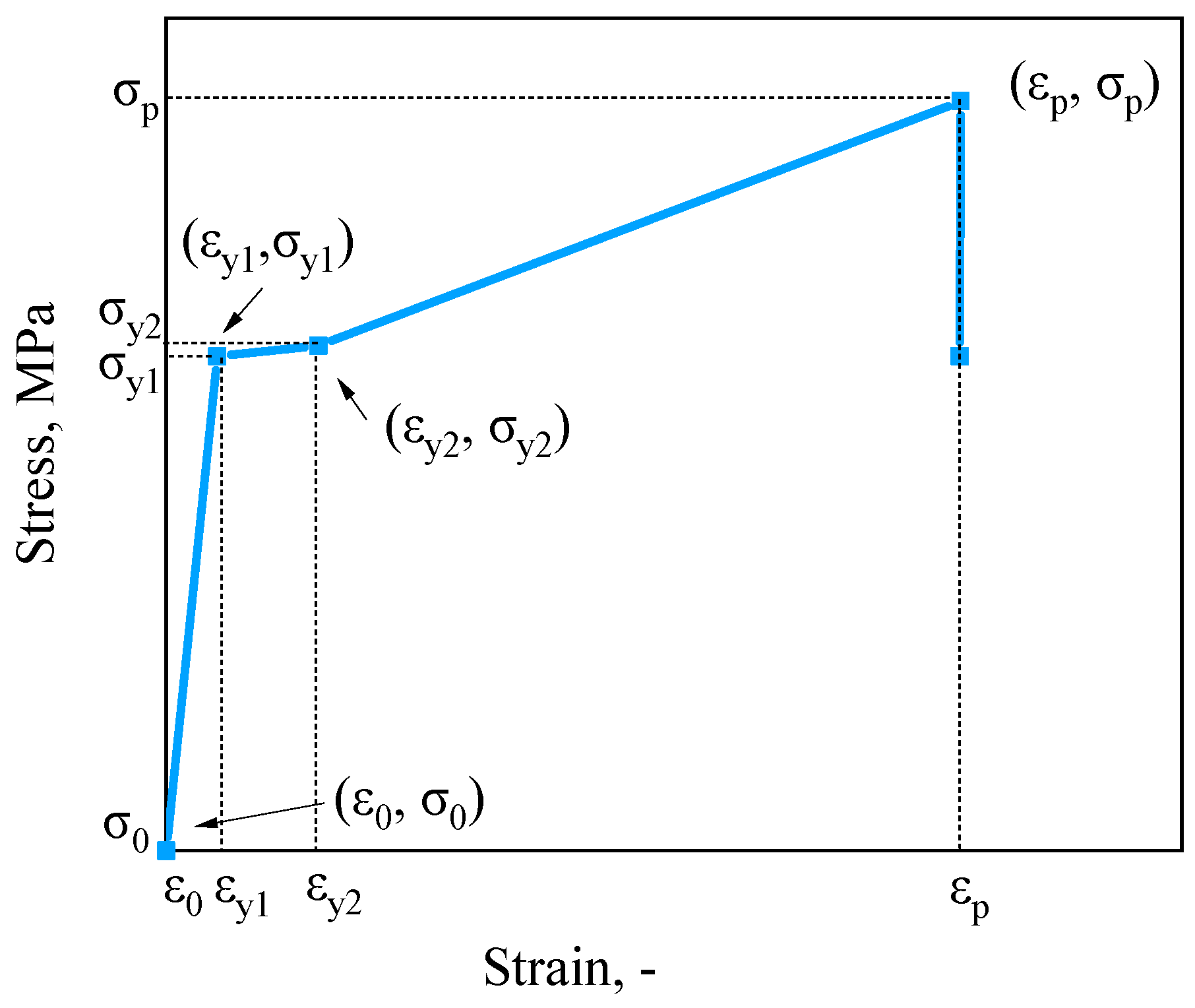
The following four points describe the tri-linear constitutive model as was initially proposed in [6]:
where is the stress at the starting point, is the strain at the starting point, is the stress at the beginning of the yielding stage, is the strain at the beginning of the yielding stage, is the stress at the beginning of the reinforcement stage, is the strain at the beginning of the reinforcement stage, is the maximum stress at the reinforcement section, is the strain at the maximum stress at the reinforcement section. A bilinear material behaviour may be described, as seen in Figure 13.
Figure 9.
Bilinear elasto-plastic stress–strain relationship.
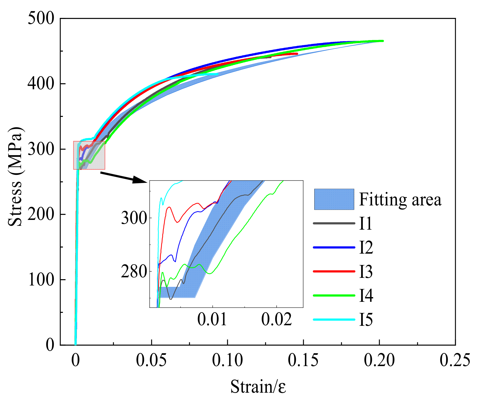
The average thickness remaining ratio range for specimens in each zone is substituted into Eq. (17) to obtain the fitting regions for the tri-linear constitutive model. A comparison between the areas fitted and the experimental stress-strain curves is shown in Figure 14. For the splash zone, the duration of the elastic stage in the observed data aligns closely with the fitting region, the yield stage is slightly above the fitting region, with a maximum difference of 0.9%, and the strengthening stage matches the fitting region at both ends but shows a slight elevation in the middle part of the experimental data. The overall situation in the tidal zone is like the splash zone, with a maximum difference of 3.3% in the duration of the elastic stage. The immersion zone closely resembles the first two zones in the elastic stage, with a maximum difference of 3.8% in the duration of the elastic stage. The strengthening stage for most of the experimental data is slightly above the fitting region but with minimal differences. Comparing the experimental stress-strain curves and the formula-fitted areas for the three zones, it is observed that the plastic and strengthening stages in the middle part are somewhat conservative. In contrast, the other regions are almost identical, with a maximum difference of 5%.
Figure 10.
True stress-strain curves, splash (left) and tidal (right) zones.
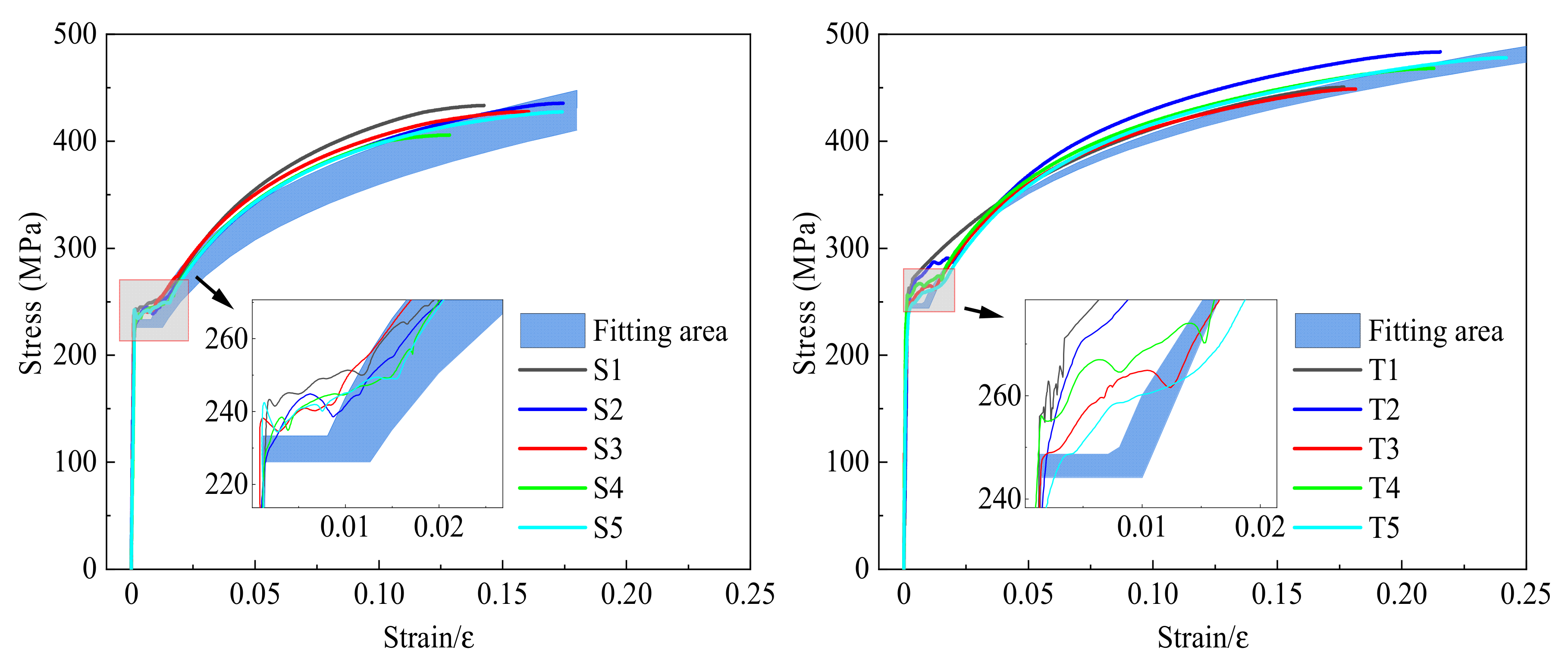
Figure 11.
True stress-strain curves, immersion zone.
5. Corrosion degradation allowance
Corrosion degradation is a time-dependent, non-linear process, and its development involves different stages, resulting in various forms of degradation. Corrosion degradation may be global uniform, local pitting, crevice, galvanic, and fatigue corrosion [30,31]. The corrosion rate and depth can be predicted by employing corrosion degradation models, which can be used for the structural reliability of steel structures during the service life. The currently used corrosion models may be classified as linear, exponential, power-law, and Weibull models corrosion [32,33,34,35,36,37,38,39,40].
Guedes Soares & Garbatov [41] developed a non-linear model for describing corrosion growth, where the entire corrosion degradation process is divided into three stages, as shown in Figure 15. In the first stage, t[O, A], the structure does not experience corrosion degradation due to the corrosion protection system. The second stage, t[A, B], begins after the corrosion protection system fails. The third stage, t[B, ], occurs as corrosion products adhere to the structure’s surface, preventing further corrosion development. The corrosion process gradually stops, and the corrosion rate approaches zero. However, corrosion degradation will restart if the corrosion layer detaches from the metal’s surface due to scouring or other human activities.
Figure 12.
Corrosion depth as a function of time [41].
Figure 12.
Corrosion depth as a function of time [41].
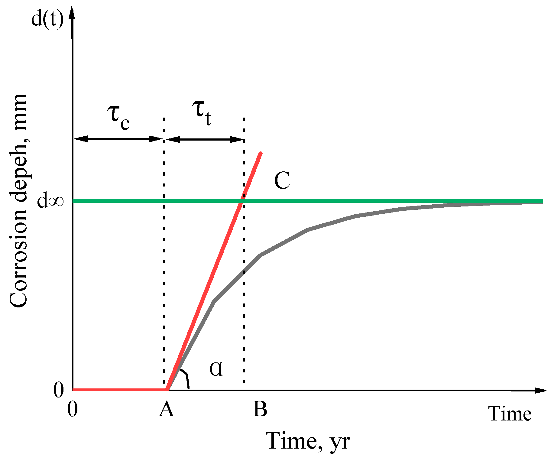
Corrosion measurement activities were conducted around the 5th year of the service life, and the steel pipe piles had already undergone severe corrosion degradation, resulting in a thickness reduction. It is assumed that once corrosion forms a relatively deep corrosion layer, preventing oxygen from reaching the fresh material, the corrosion degradation rate will decrease or even stop until the corroded layer is penetrated or cleaned. Given the comprehensive corrosion protection design and corrosion prevention measures, the coating life is assumed = 1 year. The transition time, in the corrosion thickness model [4,41] is defined based on the experimental result, the long-term corrosion thickness achieved by = 5 years is assumed as = 6.00, mm. The mean value corrosion depth based on the two models used here are (see Figure 16) presented as:
Linear model:
where years is the time of the corrosion depth measurement campaign. The exponential model requires regular measurement campaigns during the service life. The second model is based on an individual measurement campaign, which can be done at any time once the corrosion propagates. The two corrosion degradation models analysing the analysed zones are shown in Figure 13 and Figure 14. The transition time is estimated based on the corrosion depth measurements accounting for the coating life and long-term corrosion depth. Table 9 shows the transition times for different zones.
Figure 13.
Corrosion degradation in tidal (left) and splash zones.
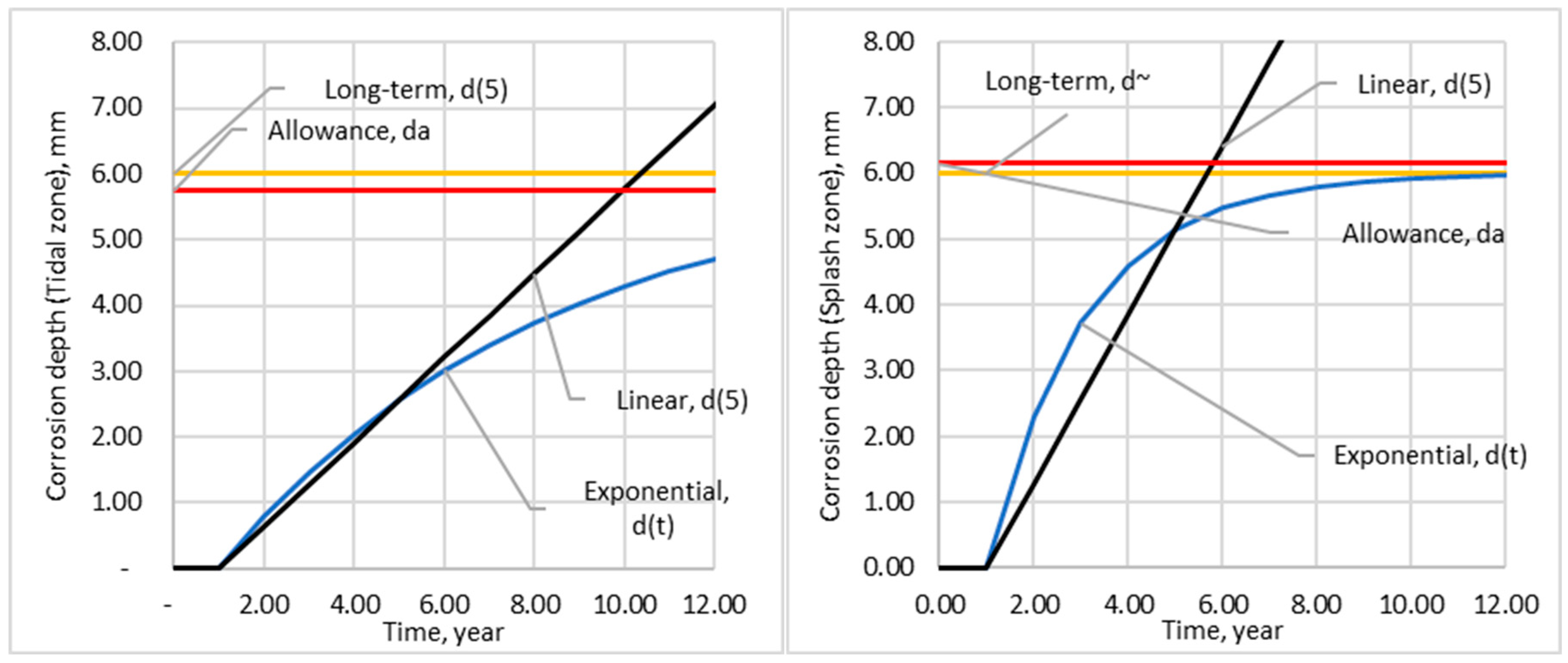
Figure 14.
Corrosion degradation in immersed zone.
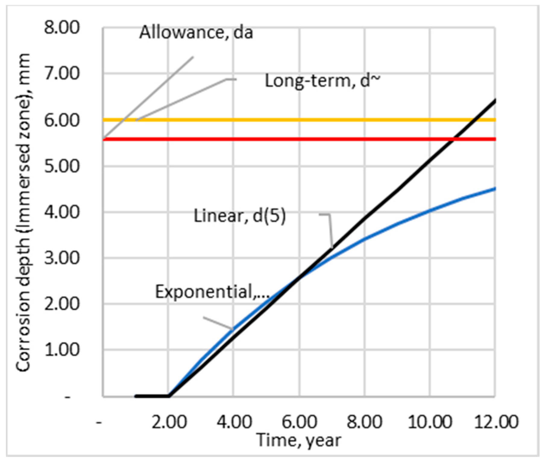

Table 9.
Transition time.
|
|
, years | |
|---|---|---|
| S-zone | 5.13 | 2.07 |
| T-zone | 2.65 | 7.17 |
| I-zone | 2.56 | 7.17 |
It can be seen from Table 9 that the transition time of the splash zone is much shorter, and the corrosion degradation is much more profound. It has already been proven [39] that the logarithms relationship can be used to describe the standard deviation as a function of the time as:
where is 0.12, 0.15 and 0.02 for S, T and I-zones respectively.
The corrosion wastage allowances can be defined using the beta structural reliability index at the end of the service life using FORM [42,43]. When estimating corrosion wastage allowances, all significant inherent (aleatory) variability is accounted for in the long-term analysis in predicting the corrosion depth progress during the service life. Epistemic (lack of knowledge) type of uncertainties will, in most cases, be assumed to be covered by the partial safety factor.
The limit state function, for estimating the corrosion wastage allowances at the end of the service life of 20 years, is defined as:
where is the wastage allowance, is the corrosion depth estimated at the 20th year and the design equation is given as:
The beta reliability index at the end of the service life is defined by FORM as . Using statistical descriptors of and the prediction of the corrosion degradation at the 20th year of the service life, Eqns (22) and (24), the design points of and in the normal design space of FORM can be defined, and once the convergence is achieved, the partial factors are calculated as:
Finally, the mean value of the corrosion wastage allowances accounting for the beta reliability index at the end of the service life is defined as:
Table 10 shows the partial factors and corrosion wastage allowances.
The corrosion wastage allowances should be added to the pile net thickness in the different corrosion environment zones during the design process to guarantee that the structural behaviour of the corroded pile at the year 20 will be with the predicted reliability level. The wastage allowances are based on the corrosion degradation measurements conditional on the environmental conditions and beta structural reliability [44].
6. Conclusions
This study investigated the mechanical properties of steel pipe piles subjected to severe marine corrosion environments explored during the last five years. The study analyses the loss rates of steel material mechanical properties in the splash, tidal, and fully submerged zones, comparing them with specimens subjected to alternative corrosion methods to assess the degree of mechanical degradation. Experimental results reveal that the steel piles in the splash zone undergo the most severe corrosion, with average loss rates of 23.5% for yield strength, 8.8% for ultimate tensile strength, 31.9% for elongation at break, and 19.9% for elastic modulus. Comparing the degradation of elastic modulus and yield strength for different steel types in various marine corrosion environments, it was observed that the differences in mechanical performance degradation among other steels are minimal. Elastic modulus degradation is more consistent across different environments and is particularly pronounced in the splash zone. The developed regression equations are suitable for predicting the mechanical performance of steel pile materials in areas with more severe corrosion. The probabilistic design solutions developed for the corrosion thickness allowance for different corrosion environments referred to a specific service period and reliability level. The developed approaches are flexible in estimating the mechanical properties and corrosion allowance, where any further update in collecting more data may result in a different trend in the present study’s estimated mechanical properties and corrosion allowances.
Author Contributions
RX: Investigation, Formal analysis, Test, Writing- Original draft preparation; YG: Supervision, Methodology, Formal analysis, Writing- Reviewing and Editing; CL: Methodology, Supervision, Writing- Reviewing and Editing; MS: Test, Data Curation, Conceptualization. All authors have read and agreed to the published version of the manuscript.
Acknowledgments
The authors would like to thank the China Scholarship Council for help with Funding. The second author has been supported by the Strategic Research Plan of the Centre for Marine Technology and Ocean Engineering, financed by the Portuguese Foundation for Science and Technology (Fundação para a Ciência e Tecnologia - FCT) under contract UIDB/UIDP/00134/2020.
Conflicts of Interest
The authors declare no conflict of interest.
References
- Wang, K.; Zhao, M. Mathematical model of homogeneous corrosion of steel pipe pile foundation for offshore wind turbines and corrosive action. Adv Mater Sci Eng. 2016, 9014317. [Google Scholar] [CrossRef]
- Alcántara, J.; Chico, B.; Simancas, J.; Díaz, I.; Morcillo, M. Marine atmospheric corrosion of carbon steel: a Review. Materials 2017, 10, 406. [Google Scholar] [CrossRef] [PubMed]
- Appuhamy, J.; Kaita, T.; Ohga, M.; Fujii, K. Prediction of residual strength of corroded tensile steel plates. Int J Steel Struct. 2011, 11, 65–79. [Google Scholar] [CrossRef]
- Garbatov, Y.; Guedes Soares, C.; Parunov, J.; Kodvanj, J. Tensile strength assessment of corroded small-scale specimens. Corros. Sci. 2014, 85, 296–303. [Google Scholar] [CrossRef]
- Garbatov, Y.; Parunov, J.; Kodvanj, J.; Saad-Eldeen, S.; Guedes Soares, C. Experimental assessment of tensile strength of corroded steel specimens subjected to sandblast and sandpaper cleaning. Marine Structures 2016, 49, 18–30. [Google Scholar] [CrossRef]
- Garbatov, Y.; Guedes Soares, C.; Parunov, J. Fatigue strength experiments of corroded small scale steel specimens. Int J Fatigue 2014, 59, 137–144. [Google Scholar] [CrossRef]
- Yang, H.; Zhang, Q.; Tu, S.; Wang, Y.; Li, Y.; Huang, Y. A study on a time-variant corrosion model for immersed steel plate elements considering the effect of mechanical stress. Ocean. Eng. 2016, 125, 134–146. [Google Scholar] [CrossRef]
- Yang, H.; Zhang, Q.; Tu, S.; Wang, Y.; Li, Y.; Huang, Y. Effects of inhomogeneous elastic stress on corrosion behaviour of Q235 steel in 3.5% NaCl solution using a novel multi-channel electrode technique. Corros. Sci. 2016, 110, 1–14. [Google Scholar] [CrossRef]
- Sheng, J.; Xia, J. Effect of simulated pitting corrosion on the tensile properties of steel. Constr. Build. Mater. 2017, 131, 90–100. [Google Scholar] [CrossRef]
- Zhang, J.; Shi, X.H.; Guedes Soares, C. Experimental analysis of residual ultimate strength of stiffened panels with pitting corrosion under compression. Eng Struct. 2017, 152, 70–86. [Google Scholar] [CrossRef]
- Jia, C.; Shao, Y.; Guo, L.; Liu, Y. Incipient corrosion behaviour and mechanical properties of low-alloy steel in simulated industrial atmosphere. Constr. Build. Mater. 2018, 187, 1242–1252. [Google Scholar] [CrossRef]
- Gathimaba, N.; Kitane, Y.; Yoshida, T.; Itoh, Y. Surface roughness characteristics of corroded steel pipe piles exposed to marine environment. Constr. Build. Mater. 2019, 203(10), 267–281. [Google Scholar] [CrossRef]
- Zhang, L.; Jiang, L.; Zhang, Z.; Wang, Y.; Qiu, L. Study on tensile properties of Q235nh after corrosion. Steel Construction (Chinese & English), 2019; 37, 1–7. [Google Scholar] [CrossRef]
- Guo, Q.; Zhao, Y.; Xing, Y.; Jiao, J.; Fu, B.; Wang, Y. Experimental and numerical analysis of mechanical behaviours of long-term atmospheric corroded Q235 steel. Structures 2022, 39, 115–131. [Google Scholar] [CrossRef]
- Xia, R.; Jia, C.; Liu, C.; Liu, P.; Zhang, S. Non-uniform corrosion characteristics of the steel pipe pile exposed to marine environments. Ocean. Eng. 2023, 272, 113873. [Google Scholar] [CrossRef]
- Woloszyk, K.; Garbatov, Y.; Klosowski, P. Stress–strain model of lower corroded steel plates of normal strength for fitness-for-purpose analyses. Constr. Build. Mater. 2022, 323, 126560. [Google Scholar] [CrossRef]
- Woloszyk, K.; Garbatov, Y. Random field modelling of mechanical behaviour of corroded thin steel plate specimens. Eng Struct 2020, 212, 110544. [Google Scholar] [CrossRef]
- Garbatov, Y.; Guedes Soares, C. Spatial Corrosion Wastage Modeling of Steel Plates Exposed to Marine Environments. J Offshore Mech Arct. 2019, 141, 031602. [Google Scholar] [CrossRef]
- Woloszyk, K.; Garbatov, Y. Advanced numerical modelling for predicting residual compressive strength of corroded stiffened plates. Thin Wall Struct. 2023, 183, 110380. [Google Scholar] [CrossRef]
- Garbatov, Y. Fatigue strength assessment of ship structures accounting for a coating life and corrosion degradation. International Journal of Structural Integrity 2016, 7, 305–322. [Google Scholar] [CrossRef]
- Garbatov, Y.; Sisci, F.; Ventura, M. Risk-based framework for ship and structural design accounting for maintenance planning. Ocean. Eng. 2018, 166, 12–25. [Google Scholar] [CrossRef]
- Zayed, A.; Garbatov, Y.; Guedes Soares, C. Corrosion degradation of ship hull steel plates accounting for local environmental conditions. Ocean. Eng. 2018, 163, 299–306. [Google Scholar] [CrossRef]
- Gong, M. Metal corrosion theory and corrosion control. Chemical Industry Press, 2018.
- Removal of Corrosion Products from Corrosion Specimens of Metals and Alloys: GB/T 16545-2015. Beijing: Standards Press of China, 2015.
- Carbon Structural Steel: GB/T 700-2006. Beijing: Standards Press of China, 2006.
- Metallic Materials—Tensile Testing—Part 1: Method of Test at Room Temperature: GB/T 228.1—2010. Beijing: Standards Press of China, 2010.
- Garbatov, Y.; Guedes Soares, C. Experimental evaluation of ageing marine structures. SNAME Maritime Convention and 5th World Maritime Technology Conference 2015, D021S005R008. [Google Scholar] [CrossRef]
- Bai, P.; Ni, Y.; Lei, D. Measurement of true stress-strain relationship of stainless steel based on digital image correlation technique. Science Technology and Engineering 2020, 20, 5240–5246. [Google Scholar] [CrossRef]
- Chen, R.; 2022. Research on the degradation of steel structures for the needs of structural life-cycle design and time-dependent reliability in corrosive environment. Southeast University, 2022. [CrossRef]
- Woloszyk, K.; Garbatov, Y. Advances in Modelling and Analysis of Strength of Corroded Ship Structures. J. Mar. Sci. Eng. 2022, 10, 807. [Google Scholar] [CrossRef]
- Marchese, S.S.; Epasto, G.; Crupi, V.; Garbatov, Y. Tensile Response of Fibre-Reinforced Plastics Produced by Additive Manufacturing for Marine Applications. J. Mar. Sci. Eng. 2023, 11, 334. [Google Scholar] [CrossRef]
- Garbatov, Y.; Saad-Eldeen, S.; Guedes Soares, C.; Parunov, J.; Kodvanj, J. Tensile test analysis of corroded cleaned aged steel specimens. Corrosion Eng Sci Techn. 2018, 54, 154–162. [Google Scholar] [CrossRef]
- Melchers, R. Probabilistic Modelling of Marine Corrosion of Steel Specimens. In Proceedings of the 5th International Offshore and Polar Engineering Conference; 1995; pp. 204–210. [Google Scholar]
- Melchers, R.E. Modelling of Marine Corrosion of Steel Specimens. Corrosion Testing in Natural Waters 1997, 2, 20–23. [Google Scholar]
- Yamamoto, N.; Ikagaki, K. A Study on the Degradation of Coating and Corrosion on Ship´s Hull Based on the Probabilistic Approach. J Offshore Mech Arct. 1998, 120, 121–128. [Google Scholar] [CrossRef]
- Melchers, R.E. Probabilistic Modelling of Immersion Marine Corrosion. In Structural Safety and Reliability; Shiraishi, N., Shinozuka, M., Wen, Y., Eds.; Balkema, 1998; pp. 1143–1149. [Google Scholar]
- Yamamoto, N.; Yao, T. Hull girder strength of a tanker under longitudinal bending considering strength diminution due to corrosion. In Proceedings of the Structural Safety and Reliability, 8th International Conference (ICOSSAR2001); 2001. [Google Scholar]
- Zayed, A.; Garbatov, Y.; Guedes Soares, C. Corrosion modelling of single hull crude oil tanker subjected to multiple deterioration environments. In Proceedings of the 26th International Conference on Offshore Mechanics and Arctic Engineering; 2007; p. Paper OMAE2007-29741. [Google Scholar]
- Silva, J.E.; Garbatov, Y.; Guedes Soares, C. Reliability assessment of a steel plate subjected to distributed and localised corrosion wastage. Eng Struct 2014, 59, 13–20. [Google Scholar] [CrossRef]
- Jurišić, P.; Parunov, J.; Garbatov, Y. Aging Effects on Ship Structural Integrity. Brodogradnja 2017, 68, 15–28. [Google Scholar] [CrossRef]
- Guedes Soares, C.; Garbatov, Y. Reliability of maintained, corrosion-protected plates subjected to non-linear corrosion and compressive loads. Mar. Struct. 1999, 12, 425–445. [Google Scholar] [CrossRef]
- Rackwitz, R. First order reliability theories and stochastic models. In Proceedings of the International conference ICOSSAR’77I, Munich, Germany, 19–21 September 1977. [Google Scholar]
- Gollwitzer, S.; Rackwitz, R. First-Order System Reliability of Structural Systems. In Proceedings of the 4th International Conference on Structural Safety and Reliability, Kobe, Japan, 27–29 May 1985; pp. 171–218. [Google Scholar]
- Garbatov, Y. Risk-based corrosion allowance of oil tankers. Ocean. Eng. 2020, 213, 107753. [Google Scholar] [CrossRef]
Figure 1.
Steel frame of Pingtan Cross-sea Bridge.
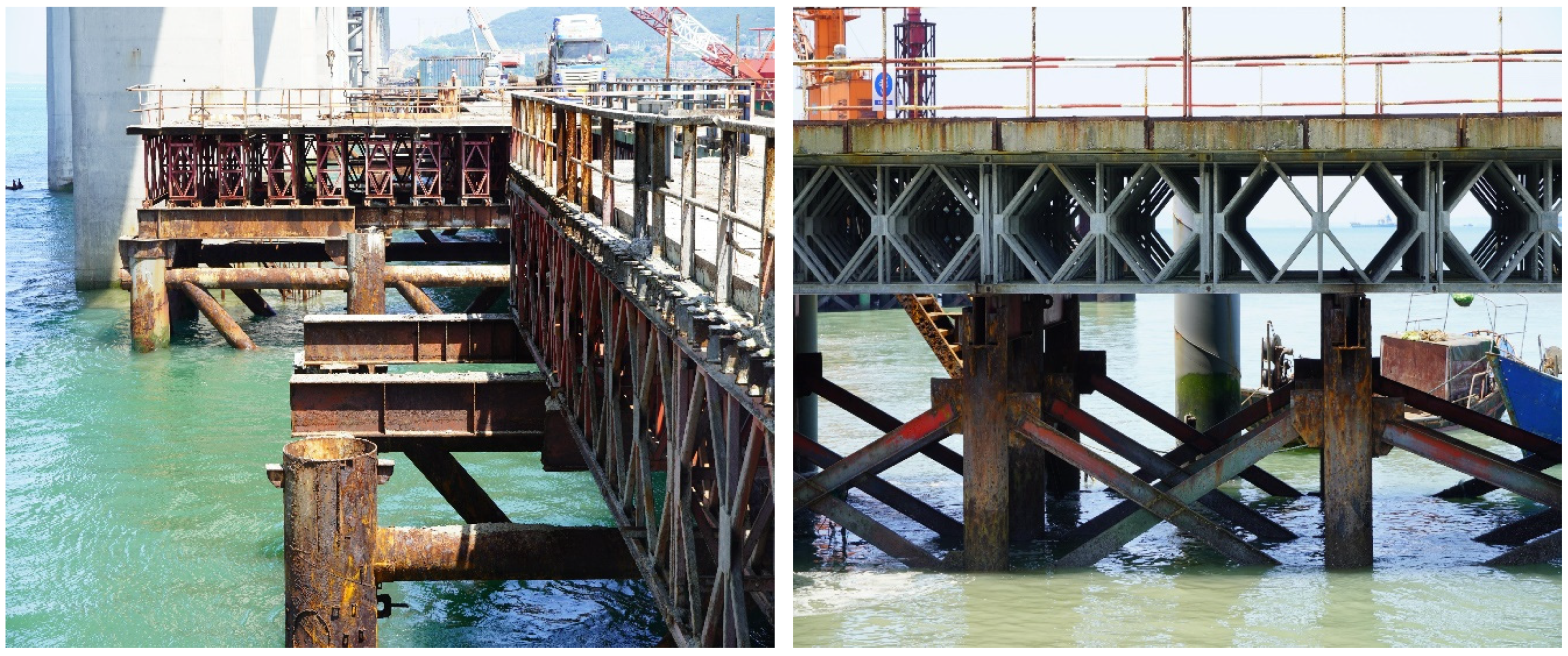
Figure 2.
Steel pipe pile and specimen locations.
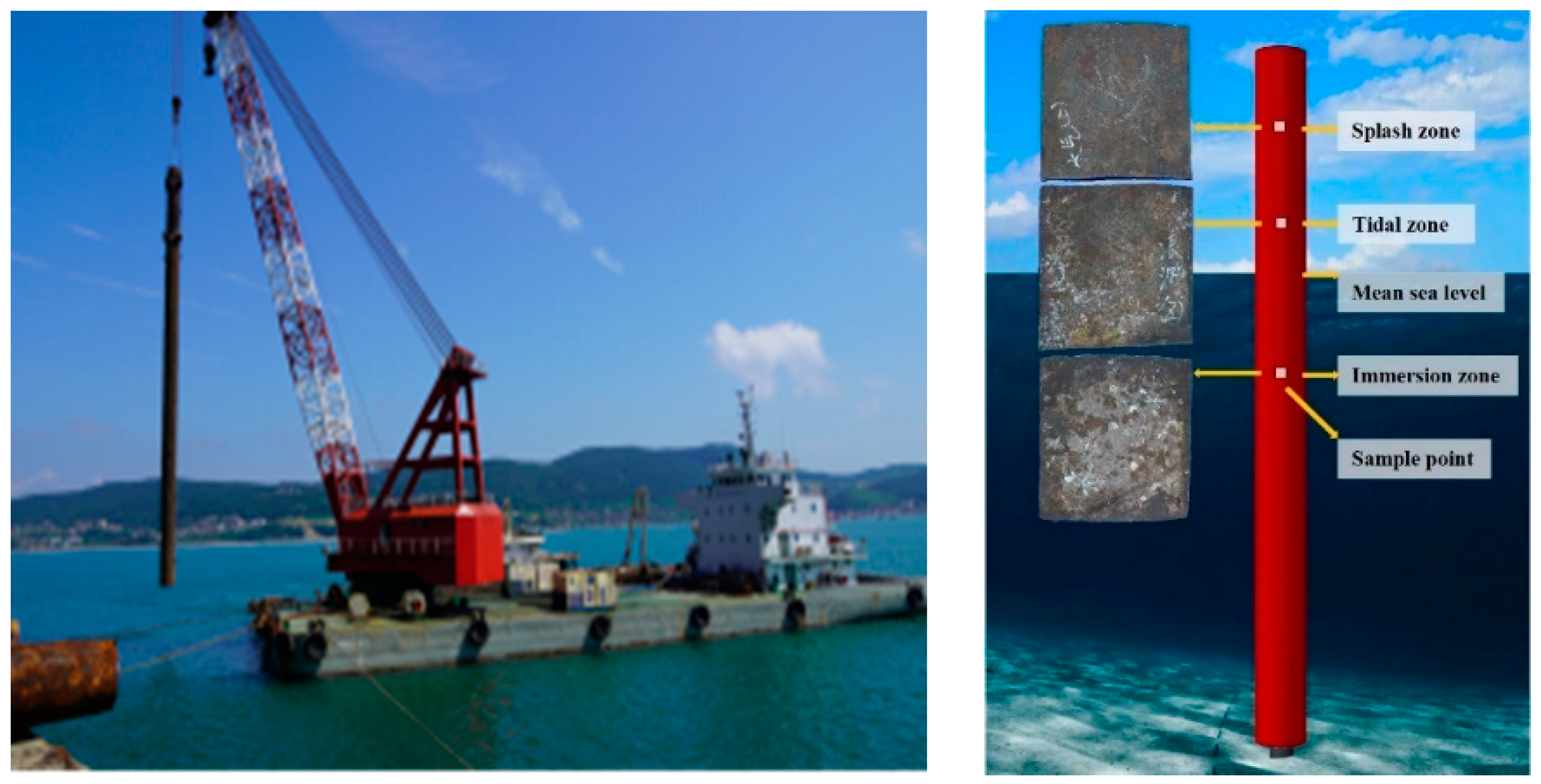
Figure 3.
Corrosion product cleaning, splash zone (left), tidal zone (central) and immersion (right) zones.
Figure 3.
Corrosion product cleaning, splash zone (left), tidal zone (central) and immersion (right) zones.
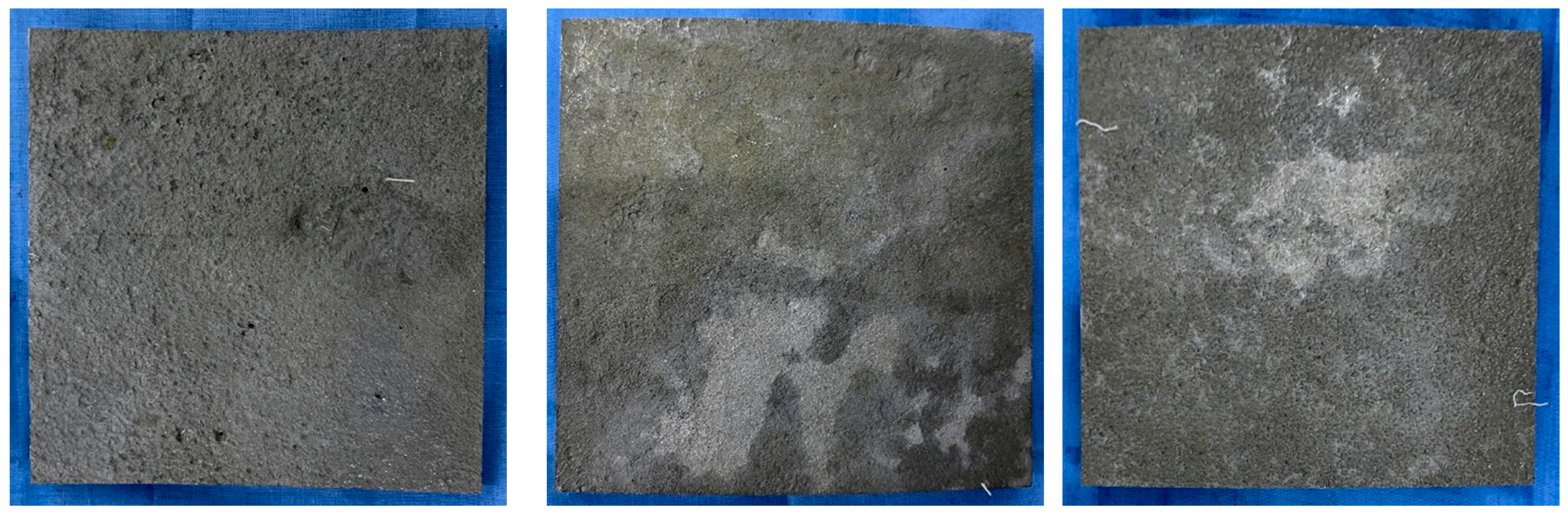
Figure 4.
Test specimen configuration.
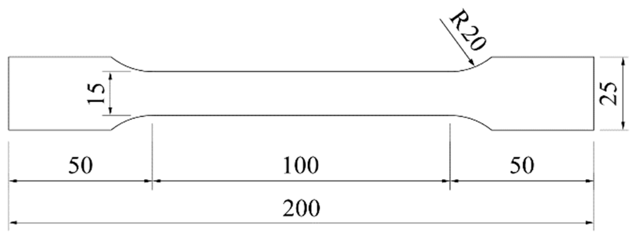
Figure 5.
Tensile test ruptured specimen.
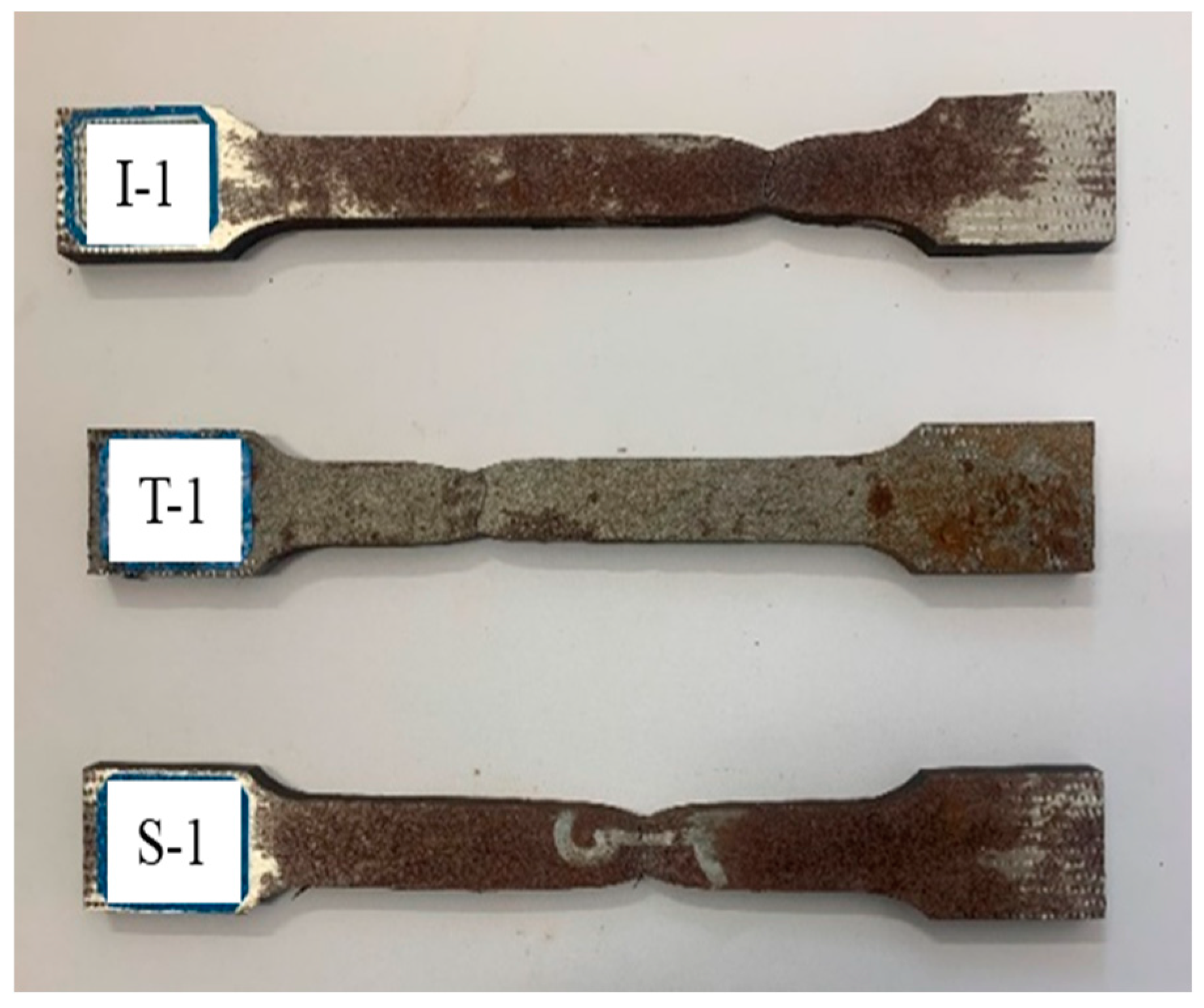
Figure 6.
Engineering stress-train curves.
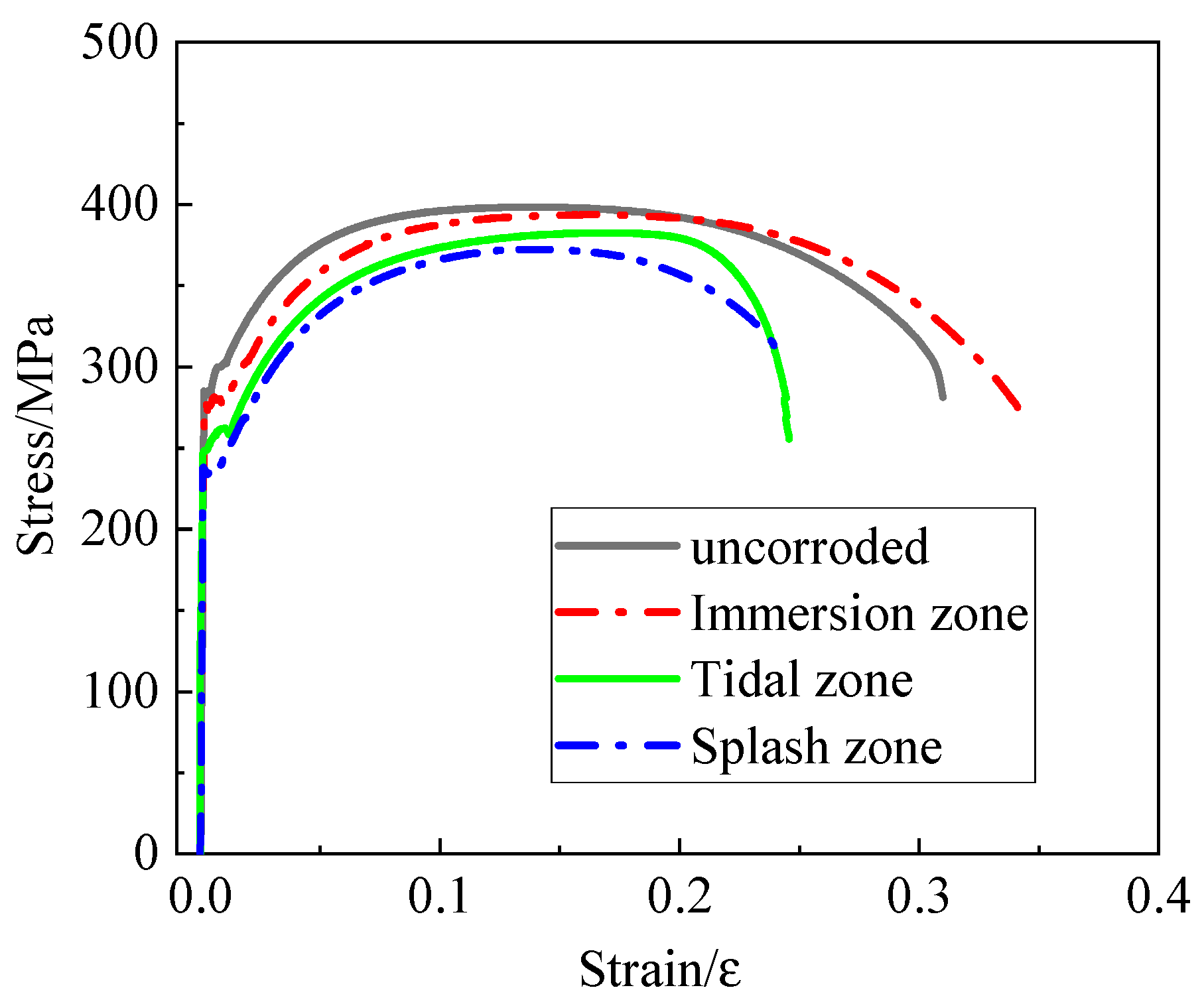
Figure 7.
True stress-strain curves of the specimens.
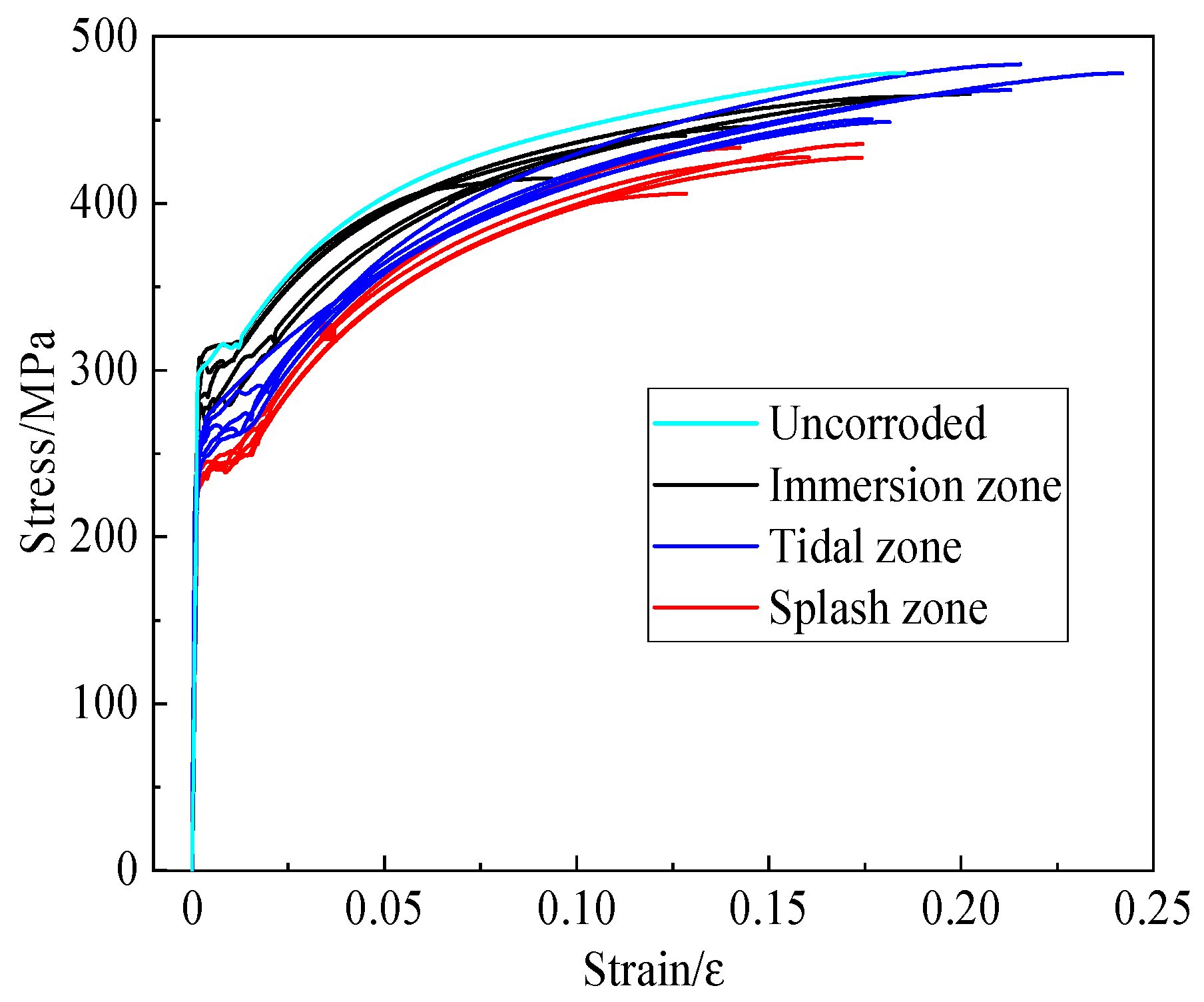
Figure 8.
Elastic modulus (left) and yield strength (right).
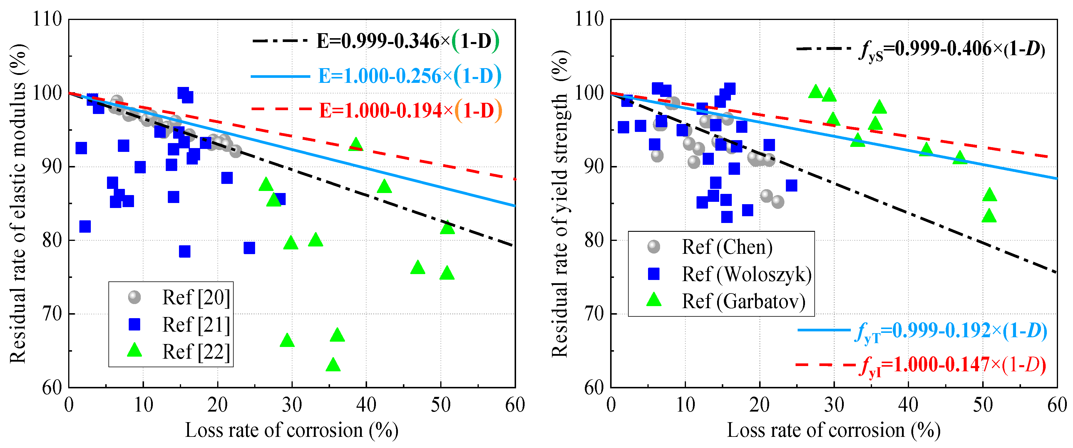
Table 1.
Marine environment characteristics in the Pingtan area.
| Characteristic | Value |
|---|---|
| Mean tidal range, m | 4.3 |
| Water temperature, °C | 19.4 |
| Maximum water velocity, m/s | 2.23 |
| Average water velocity, m/s | 1.03 |
| Dissolved oxygen saturation, % | 95-100 |
| PH | 8.1-8.3 |
| Salinity, % | 3.0-3.2% |
| Average wind velocity, m/s | 6.9 |
| Tidal cycle, times/day | 2 |
| The most enormous wave height in history, m | 16 |
Table 2.
Elemental composition of Q235B steel.
| Composition | C | Si | Mn | P | S |
|---|---|---|---|---|---|
| Content/% | 0.176 | 0.198 | 0.5 | 0.023 | 0.019 |
| GB/T 700-2006 | ≤0.20 | ≤0.35 | ≤1.40 | ≤0.045 | ≤0.045 |
Table 3.
Specimens characteristics.
| Zone | Specimen | , mm | , % | Mean, mm/ Var, mm2 |
|---|---|---|---|---|
| Splash | S-1 | 6.972 | 58.1 | 57.24/ 0.0143 |
| S-2 | 6.979 | 58.2 | ||
| S-3 | 6.877 | 57.3 | ||
| S-4 | 6.691 | 55.8 | ||
| S-5 | 6.815 | 56.8 | ||
| Tidal | T-1 | 9.367 | 78.1 | 77.92/ 0.0233 |
| T-2 | 9.496 | 79.1 | ||
| T-3 | 9.094 | 75.8 | ||
| T-4 | 9.356 | 78.0 | ||
| T-5 | 9.428 | 78.6 | ||
| Immersion | I-1 | 9.422 | 78.5 | 78.64/ 0.0004 |
| I-2 | 9.451 | 78.8 | ||
| I-3 | 9.429 | 78.6 | ||
| I-4 | 9.464 | 78.9 | ||
| I-5 | 9.413 | 78.4 | ||
| Intact | P-1 | 4.003 | - | - |
Table 4.
Parameters of tensile test.
| No. | , MPa | Mean, MPa/ Var, MPa2 |
, MPa | Mean, MPa/ Var, MPa2 |
, % | Mean, %/ Var, - |
105, MPa | Mean, 105 MPa/ Var, MPa2 |
|---|---|---|---|---|---|---|---|---|
| S-1 | 248.81 | 237.40/ 42.005 |
382.01 | 371.51/ 52.161 |
20.38 | 22.68/ 9.853 |
1.67 | 1.67/0.001 |
| S-2 | 236.51 | 373.06 | 22.65 | 1.68 | ||||
| S-3 | 233.90 | 372.46 | 24.10 | 1.70 | ||||
| S-4 | 233.95 | 362.70 | 19.16 | 1.63 | ||||
| S-5 | 233.81 | 367.33 | 27.12 | 1.65 | ||||
| T-1 | 254.43 | 263.00/ 104.467 |
384.82 | 390.16/ 59.854 |
25.40 | 29.35/ 23.300 |
1.71 | 1.78/0.010 |
| T-2 | 279.48 | 402.60 | 35.00 | 1.93 | ||||
| T-3 | 258.37 | 382.68 | 24.58 | 1.71 | ||||
| T-4 | 266.15 | 390.60 | 33.90 | 1.83 | ||||
| T-5 | 256.56 | 390.12 | 27.86 | 1.70 | ||||
| I-1 | 268.62 | 285.12/ 229.482 |
392.41 | 392.33/ 27.420 |
28.5 | 29.68/ 3.367 |
1.73 | 1.80/0.009 |
| I-2 | 282.41 | 398.54 | 30.99 | 1.94 | ||||
| I-3 | 296.93 | 392.89 | 24.53 | 1.76 | ||||
| I-4 | 273.46 | 393.77 | 34.56 | 1.85 | ||||
| I-5 | 304.17 | 384.04 | 29.83 | 1.72 | ||||
| P-1 | 310.13 | 407.18 | 33.3 | 2.08 |
Table 5.
Loss rate of corrosion mechanical properties.
| No. | loss rate, % | Mean, %/ Var, - |
loss rate, % | Mean, %/ Var, - |
loss rate, % | Mean %/ Var, - |
loss rate, % | Mean %/ Var, - |
|---|---|---|---|---|---|---|---|---|
| S-1 | 19.77 | 23.45/ 4.370 |
6.18 | 8.76/ 3.145 |
38.80 | 31.89/ 88.829 |
19.71 | 19.90/ 1.682 |
| S-2 | 23.74 | 8.38 | 31.98 | 19.23 | ||||
| S-3 | 24.58 | 8.53 | 27.63 | 18.27 | ||||
| S-4 | 24.56 | 10.92 | 42.46 | 21.63 | ||||
| S-5 | 24.61 | 9.79 | 18.56 | 20.67 | ||||
| T-1 | 17.96 | 15.20/ 10.866 |
5.49 | 4.18/ 3.619 |
23.72 | 11.87/ 210.164 |
17.79 | 14.64/ 23.933 |
| T-2 | 9.88 | 1.12 | -5.11 | 7.21 | ||||
| T-3 | 16.69 | 6.02 | 26.19 | 17.89 | ||||
| T-4 | 14.18 | 4.07 | -1.80 | 12.02 | ||||
| T-5 | 17.27 | 4.19 | 16.34 | 18.27 | ||||
| I-1 | 13.38 | 8.06/ 23.838 |
3.63 | 3.65/ 1.653 |
14.41 | 10.87/ 120.531 |
16.83 | 13.46/20.230 |
| I-2 | 8.94 | 2.12 | 6.94 | 6.73 | ||||
| I-3 | 4.26 | 3.51 | 26.34 | 15.38 | ||||
| I-4 | 11.82 | 3.29 | -3.78 | 11.06 | ||||
| I-5 | 1.92 | 5.68 | 10.42 | 17.31 |
Table 6.
Mechanical property.
| Zone | Average loss |
Average loss |
Average loss |
Average loss |
|---|---|---|---|---|
| S-zone | 23.45% | 8.76% | 31.89% | 19.90% |
| T-zone | 15.20% | 4.18% | 11.87% | 14.63% |
| I-zone | 8.06% | 3.65% | 10.87% | 13.46% |
Table 7.
Correlation between average thickness residual rate and mechanical properties.
| S-zone | 0.514 | 0.722 | 0.851 |
| T-zone | 0.474 | 0.770 | 0.578 |
| I-zone | 0.592 | 0.515 | 0.794 |
Table 8.
Coefficient of determination R2.
| Eqn | R2 | Eqn | R2 | Eqn | R2 | Eqn | R2 | |
|---|---|---|---|---|---|---|---|---|
| S-zone | (4) | 0.539 | (7) | 0.350 | (12) | 0.164 | (15) | 0.181 |
| T-zone | (5) | 0.189 | (8) | 0.225 | (13) | 0.154 | (16) | 0.195 |
| I-zone | (6) | 0.724 | (9) | 0.197 | (14) | 0.286 | (17) | 0.391 |
Table 10.
Corrosion wastage allowances.
| S-zone | 6.1487 | 1.0165 | 1.0082 |
| T-zone | 5.7386 | 1.0139 | 1.0151 |
| I-zone | 5.7207 | 1.0157 | 1.0102 |
Disclaimer/Publisher’s Note: The statements, opinions and data contained in all publications are solely those of the individual author(s) and contributor(s) and not of MDPI and/or the editor(s). MDPI and/or the editor(s) disclaim responsibility for any injury to people or property resulting from any ideas, methods, instructions or products referred to in the content. |
© 2023 by the authors. Licensee MDPI, Basel, Switzerland. This article is an open access article distributed under the terms and conditions of the Creative Commons Attribution (CC BY) license (https://creativecommons.org/licenses/by/4.0/).
Copyright: This open access article is published under a Creative Commons CC BY 4.0 license, which permit the free download, distribution, and reuse, provided that the author and preprint are cited in any reuse.


