
Submitted:
11 April 2025
Posted:
12 April 2025
You are already at the latest version
Abstract
The increasing frequency and intensity of heat waves, combined with urban heat islands (UHI), pose significant public health challenges. Implementing low-cost, real-time moni-toring networks with distributed stations within the Smart city framework faces obstacles in transforming urban spaces. However, accurate data is essential for assessing these ef-fects. This paper compares different network types in a medium sized city in West Spain and their implications for UHI identification quality. The study first examines a pur-pose-built monitoring network using Open-Source platforms, IoT technology, and Lo-RaWAN communications, adhering to World Meteorological Organization guidelines. Additionally, it evaluates two citizen weather observer networks (CWON): one from a commercial smart device company and another from a global community connecting en-vironmental sensor data. The findings highlight several advantages of bespoke monitor-ing networks over CWON. These networks offer enhanced data accessibility and greater flexibility to meet specific requirements, facilitating adaptability and scalability for future upgrades. However, specialization is crucial for effective deployment and maintenance. Conversely, CWON faces limitations in network uniformity, data shadow zones, and in-sufficient knowledge of real sensor situations or component characteristics. Furthermore, CWON exhibits some data inconsistencies in probability distribution and scatter plots during extreme heat periods, as well as improbable UHI temperature values.
Keywords:
IoT
; Urban Heat Islands
; LoRaWAN
; Open-Source Platforms
; Smart Cities
; Monitoring
; Digitalization
; Real Time Data
; Citizen Networks
; Automatic Weather Station
1. Introduction
Currently, more than half of the world's population lives in cities, and this figure is expected to rise to two-thirds by 2050 [1]. Given this increasing urbanization, one of the major challenges of this century is the sustainable management of urban planning and the enhancement of urban public spaces. This is with a view to improving the physical and mental health and well-being of both the collective and individual populations [2].
The necessity for effective urban administration, in conjunction with the digital revolution and the utilisation of information and communication technologies, has precipitated the metamorphosis of 'traditional cities' into 'smart cities'. These smart cities collect, integrate, and analyse a multitude of environmental data, with a view to enhancing both the quality of life for citizens and the efficiency of management and decision-making processes [3].
It is evident that a number of networks and organisations have a pivotal function in facilitating collaboration between various stakeholders for the advancement and execution of smart city technologies on a global scale: Open & Agile Smart Cities [4], Global Smart Cities Alliance [5], Programme on Smart Cities and Inclusive Growth [6], The Smart Communities Network [7]. When it comes to applying IoT in smart cities and buildings, various areas of use emerge, including mobility [8], waste management [9], healthcare [10], environment and more [11].
The monitoring of parameters pertaining to comfort and general well-being of building occupants has attained widespread development [12]. In this context, the Public Space Charter emphasises that adapting public spaces to local climatic conditions not only enhances environmental well-being but also contributes to mitigating climate change and UHI [13]. This issue has become increasingly salient due to the significant impact of climate change on urban environments. The IPCC has issued a warning regarding a projected increase in global temperatures, which is expected to result in a greater frequency and intensity of heatwaves. Consequently, this will result in a higher number of heat-related mortalities, particularly in densely populated urban areas calling for the implementation of adaptation measures [14].
Furthermore, the concept of urban heat islands must be considered. These are climate disturbances related to the difference in air temperature between urban areas and their surroundings, which mainly affect summer periods and manifest as a dynamic phenomenon of overheating [15]. The phenomenon is primarily attributable to anthropogenic activity and urban infrastructure, deforestation and shading, and the utilisation of heat-absorbing materials [16]. The findings of long-term, high-resolution global diurnal surface temperature studies indicate that there is a discrepancy between urban and rural areas regarding 3-day extremes. On average, these extremes are more than double the SUHI warm-season median, with local exceedances of up to 10 °C [17]. In small and medium-sized cities, the difference in air temperature between urban and rural areas can vary between 2 and 7 °C [18,19,20,21,22].
To define UHI, assess their impact, and develop adaptation and mitigation strategies, it is essential to study hygrothermal data. These data can be obtained from various sources, including satellite, meteorological, climatological, statistical, and Earth observation [23]. The WMO provides guidelines for measuring climatic variables at different scales to ensure the accuracy, consistency, and quality of measurements from in-situ sensors (e.g., those used in weather stations) and complementary sources such as satellites, weather radars, and climate prediction models. These guidelines encompass a range of aspects, including measurement instruments (the definition of sensor requirements in terms of accuracy, consistency, quality standards, calibration, and so forth) and the measurement techniques, which encompass both manual observations (with traditional weather stations) and automated methods (with remote monitoring) [24].
A plethora of studies have analysed climate using satellite and remote sensing data, thereby enabling systematic study of SUHI [25]. Notable sources encompass MODIS [26], Landsat [27], and, though to a lesser extent, Sentinel [28]. However, the utilisation of satellite data is encumbered by inherent limitations, including but not limited to inadequate resolution, the challenge of correlating surface temperature data with temperatures within the urban canopy [29], the necessity of clear sky conditions for precise measurements, and the complexity of providing three-dimensional urban information [30]. Consequently, the utilisation of auxiliary sources, such as weather stations, as evidenced by a substantial study conducted in China, becomes imperative to substantiate remotely sensed data [31].
Furthermore, the implementation of urban sensors for the collection and analysis of weather data has been driven by networks such as Smart Cities Marketplace [32] and Smart Cities Information System [33]. The EUMETNET initiative, a European community of National Meteorological and Hydrological Services (NMHS), has promoted citizen cooperation in weather monitoring [34]. This community obtain data mainly from four sources: Netatmo, a manufacturer of smart home devices; Sencrop and WEENAT, which are used for agricultural purposes; and Weather Observations Website (WOW), which enables users to register CWS from different providers to automatically upload weather observations [35]. A substantial number of studies have employed CWON data in urban contexts for UHI studies. For instance, WU and HetWeerActueel were used to investigate urban effects on temperature and precipitation in the Netherlands [36]. Using Netatmo network, a study conducted in London reported temperature differences ranging from 1 to 6 ° C [37], whereas research in Berlin, based on observations from up to 1,500 stations over the course of a year, underscored the significance of data quality and representativeness [38]. In Vienna and Amsterdam comparisons were made with reference stations [39,40]. These studies emphasise the potential of CWSs in UHI research but underscore the necessity for rigorous quality control before using the data or integrating them into operational services. A notable finding is that CWS networks, due to their absence of quality standards and environmental condition knowledge, exhibit greater uncertainty compared to official NMHS reference stations. A range of quality control procedures have been the subject of study; notably, A. Napoly et al. [41] developed a statistically based quality control system for crowdsourced air temperature data.
Other experiences are based on deploying their own networks to provide CWS availability in a particular area or density. Several notable instances of success with commercial devices have been documented. In Taiwan, mobile transect measurements were combined with fixed stations using low-cost sensors [42]. A similar approach was adopted in Chile, where critical areas with UHI intensities ranging from 0.5 °C to 13 °C were identified [43]. In Rome, a study utilised monthly maximum and minimum climate data from urban fixed stations and reference airport stations to dynamically simulate the impact on building energy performance, with maximum UHI intensities ranging from 3.1 °C during the day to 3.5 °C at night [44]. Regarding the use of proprietary networks and self-created stations, the study conducted in Taipei aimed to analyse the impact of vehicular traffic on UHI intensity, by employing stations specifically designed with high-precision sensors protected from solar radiation, Arduino-based devices and placed between 3 and 4.5 meters above ground level [45]. Arduino was also used in London to determine if low-cost sensors could detect small-scale temperature variations [46]. The Birmingham Urban Climate Laboratory provides an overview of the logistical aspects of implementing an urban weather network, including the selection of suitable locations, equipment testing and calibration, quality control mechanisms, and the use of existing Wi-Fi networks for data transmission [47].
Furthermore, there are other issues that have received less attention. These include the selection of IoT communication protocols that will improve range, data transmission speed, energy efficiency, and cost [48]. The utilisation of RTD, which is pivotal for smart city networks [49], and the implementation of scalable information system architecture and open-source hardware and software should be incorporated into any current network.
Moreover, the quality of RTD network records based on low-cost stations for UHI identification has not been systematically verified [38]. While CWSs are fundamental for collecting urban climate data, sensor precision variability, station location differences, and lack of standardization in data collection methods can affect the reliability of results [50].
Consequently, there is a necessity for verification against WMO standards in order to identify areas for improvement and develop best practices in urban monitoring [51]. Despite the fact that the WMO provides recommendations for measuring climatic variables, there is a paucity of detailed documentation on the design and implementation process in specific environments, which limits replicability in other cities.
2. Materials and Methods
The main objective of this article is to compare the characteristics (components, performance and placing of measuring points), value and quality of the registers of numerous RTD monitoring networks made up of low-cost devices, currently used to identify UHI in research. In addition, the following specific objectives are also considered:
- To describe the research process for the design and implementation of a purpose-built monitoring network to measure the UHI in the city of Cáceres. This procedure can also serve as a model for other implementations.
- To review the characteristics of the principal CWON, and the Citizen Weather Stations (CWS) incorporated in them, which supply urban temperature data for the city of Cáceres.
- To compare the characteristics of the abovementioned networks with the recommendations of the WMO concerning climatic measurements taken in urban environments.
2.1. Materials
This research work is based on the study of the RTD networks for measuring urban temperatures in Cáceres, a medium sized city in West Spain of around 96,000 inhabitants [52] and a surface area of around 2,300 hectares, over a typical period of extreme heat between August 1st and 26th, 2024.
On the one hand, a bespoke network is studied. This is made up of 25 AWSs and was deployed in July 2024 by researchers from the Polytechnic School of Cáceres as part of the project Heat Waves and Cities: Adaptation and Resilience of the Built Environment [53]. One of the principal specific objectives was the digital modelling of the city through low-cost, open-source and continuous monitoring.
On the other hand, two CWON were analysed. These are collaborative systems through which private users or organizations (such as educational institutions, meteorological organizations and other entities) can install and use commercial AWS, usually low cost, to generate a climate database accessible to both researchers and the general public [34]. In this study, the two CWON selected have the greatest number of devices deployed around the city. The two networks are first, that of the commercial enterprise Netatmo, with 14 AWSs in the city. This enterprise is specialized in the creation of intelligent devices for the home and their integration into their own system [54,55]. The second network belongs to the Weather Underground network platform [56], with 10 AWSs in the city from different manufacturers and of differing types. This network provides data concerning hyperlocal air quality and other meteorological data through the information from CWSs. Other CWON, such as Meteoclimatic [57], Noromet [58] and NCEI [59], were discarded due to their low or null presence in the city.
The density of the measuring devices of these networks in the city oscillates between approximately three units and one unit per 200 Ha., respectively. This supposes homogeneously distributed squares or grids measuring between 800 by 1,400 m.
2.2. Methods
The methodology used first evaluates the characteristics of the three networks mentioned above, with respect to the determining considerations of the ‘Guide to Instruments and Methods of Observation’ (WMO) for systems measuring urban climate data. This guide [60] provides guidance and specific recommendations based on national and international norms and the specific bibliography. This first part is structured following the order, terminology and constituent parts of the monitoring systems proposed by the said guide: choice of components and system programming (section 3) followed by the placing and installation of the measuring devices (section 4). Each section first details the most relevant specific considerations of the WMO with respect to each of the questions, later contextualizing them for each of the networks. This work examines, on the one hand, the extent to which the monitoring systems are aligned with the recommended requisites of the WMO; and on the other, allows the characteristics of each network that define their final performance to be known and therefore the recommended scope in the use of said data for measuring UHI.
A comparative analysis is then carried out of the hourly thermal records from the meteorological stations of the three networks over the same time period, on the understanding that the said records correspond directly to the accumulated urban heat (section 5). The decision was taken not to include in this paper the analysis of the records concerning relative humidity, as these are more closely related to comfort and are, in any case, not normally used to research UHI [45,61,62]. Before carrying out the data analysis, a quality control was performed to locate those values that could possibly be considered anomalous due to isolated errors in the measuring systems and also to evaluate the consistency and uniformity of the data in the entire set of each of the networks. The analysis was carried out considering two different scenarios: first, by checking the coherence of the data between the networks through the definition of the control points, i.e., through the nearby stations belonging to the different networks (an average distance of 160 m and a maximum of 300 m), and the analysis was later contextualized within a typical period of seven days; second, by differentiating between the control zones (UCZ corresponding to the local scale, i.e., HUZ) with similar topographical altitudes and vegetation that have a sufficient density of AWSs in all three networks; in this case, a typical sub-period of seven days within the general period was used. This work allows the quality of the registers to be known, and the variability of the data obtained to be evaluated according to whether they come from one network or another.
Finally, there is a comparative discussion of the results obtained in the previous sections from the three networks, analysing the differences, as well as the scope and performance of each one for monitoring and identifying UHI in smart cities (section 6).
3. Choice of System Components and Programming
3.1. Considerations of the WMO
The WMO establishes that the principal parts of a climate data monitoring system are the AWSs and the centralized processing system. It also specifies that such scenarios as interruptions in the energy supply, security failures, adverse climatic conditions and other factors that could compromise the continuous registration of data must be foreseen and managed.
3.1.1. Automatic Weather Stations
The WMO defines an AWS as a meteorological station at which observations are made and transmitted automatically and that it must fulfil certain requirements to guarantee the quality, accuracy and representativity of the measurements, minimizing any possible distortions. It prioritises the use of the AWSs that provide RTD over those that are off-line and store data. Depending on the number of climate variables monitored, AWSs are considered to be either light (generally air temperature, relative humidity, precipitation and, sometimes, atmospheric pressure), basic (adding wind speed and direction), extended (with the additional measurement of solar radiation, sunshine duration, soil temperature, evaporation and so forth) or AWOS, (which include automatic observation of visibility, cloud-base height and present weather).
Similarly, the WMO highlights the current tendency towards low-cost AWSs, which are usually offered as compact solutions developed through electronic embedded sensors and adapted software. Three main classes are considered: Compact AWS, similar to professional meteorological stations that feature individual, calibratable instruments for each variable, housed in a cabinet with data-logging and transmission capabilities; All in one, a single unit that integrates multiple sensors, with the option to add more instruments; and Stand-alone instruments, IoT devices that use low-power networks such as Wi-Fi or Bluetooth to transmit data to centralized servers and phone add-ons.
Furthermore, the firmware can be developed by the manufacturer and stored in the memory of the CPU, thus limiting user access to certain functions, or it can be open programming, which allows the user to design and develop the software, generating more flexible platforms.
Each component is described below:
a) Sensors
To measure the basic climatic conditions, it is necessary to integrate air temperature and humidity sensors that are robust, need low maintenance, and that do not suffer distortions when recording data. They may consist of various sensors connected to data gathering units via interfaces, or independent sensors connected to a CPU. As for uncertainty and performance, for the air temperature, the WMO recommends a measuring range of -80 °C to 60 °C, with a resolution of ± 0.1 °C and a measurement uncertainty of ± 0.1 °C between -40 °C and 40 °C, and of ± 0.3 °C for other ranges. The measurement range of relative humidity should be from 0% to 100% with a measurement uncertainty of ± 1%.
b) Central Processing Unit
This centralizes the data input/output operations, as well as their conversion, processing and temporal storage, depending on the type of station and use required. The data can also be distributed among several specialized digitally connected units. As for their location, if they are situated close to the sensors, then the in-situ processing is optimized and the amount of data to be transmitted is minimized; however, protection against atmospheric and electrical failures is needed. On the other hand, placing them inside increases the cabling needs and requires signal conditioning, but it does offer a greater energy stability, as well as a controlled environment.
The CPU centralizes the programming tasks of the AWS, whose main functions are initialization, sampling, raw data conversion, message coding, quality control, local data storage, data transmission and remote diagnostics and maintenance. There are other, less frequent operations in AWS, such as the averaged measurements, the manual entry of observations, data reduction, or data visualization.
c) Peripheral equipment
This equipment complements such functions of the CPU as: continuous energy supply with 12 V accumulators or batteries (which can be rechargeable or not); temporal accuracy using RTC, which keeps the clock ticking during short power cuts, thus guaranteeing accurate readings, sampling intervals and exact timings; and the system’s quality control through incorporated testing equipment, which supervises the performance of the components of the AWS, providing visual information available locally or sent to the CPU for analysis, thus facilitating both predictive and corrective maintenance.
d) Auxiliary elements
In order to ensure that the measuring devices reflect the true temperature of the environment, it is best to use radiation screens or shields as they allow the free circulation of the air, thus maintaining a uniform internal temperature equivalent to that of the surrounding air. These screens exclude radiant heat, precipitation and other phenomena, minimizing errors and accidental damage. A screen with a high thermal conductivity, such as a metal, dark colours and sizes smaller than 200 mm in diameter and 250 mm in height, will result in a poorer performance. There should be forced or natural ventilation to favour the convective process within the radiation screen.
3.1.2. Centralized System for Processing the Data from the Networks
The data collected by the AWS can be processed locally, in the AWS itself, or in a central processor of the net. In a complex meteorological network, the centralized processing system receives the data that the AWSs transmit via various means; it acquires them, decodes them, supervises their quality, processes and stores them, and finally transfers them, permitting their visualization. Furthermore, it can remotely control the AWS. Powerful computers integrated in the local networks are used to distribute the tasks efficiently.
Centralized processing facilitates the transmission and management of the data through a central system that optimizes such tasks as complex calculations and codification, thus alleviating the load on the AWS; however, such a specification (functional and technical) requires multidisciplinary collaboration.
3.2. Bespoke Network
An architecture divided into five layers is presented, ranging from the AWSs to the internal VM. The network of AWSs captures and sends data to a central node, from where users can consult the data. This data transfer is carried out using LoRaWAN technology, a long-range, low energy consumption open-source protocol. In addition, it provides high data transmission security by encrypting packets at network and application level, which means that the measuring devices can only be read by authorised servers that have registered the devices with their corresponding keys. (Figure 1)
3.2.1. Automatic Weather Stations
A stand-alone AWS RTD has been designed, which is both light (measuring temperature and relative humidity) and made to measure, in collaboration with the enterprise Electronic Engineering iRay [63] (Figure 2). The components, listed below, are mounted on a stainless-steel sheet 316, 2 mm thick, which allows easy placing and removal.
a) Sensors
A high performance sensor is used for temperature (from −40 °C to 125 °C, with an accuracy of ± 0.1 °C from 20 °C to 60 °C and of ± 0.2 °C in the rest) and for relative humidity (from 0% to 100%, typical accuracy of ± 1.5% from 0% to 80% and of ± 2.0% in the rest), with double insulation against water and dust (Sensirion SHT35 [64]). Measurements have a resolution of 0.1 °C and 0.1%, respectively. Given that the SHT35 sensor is of the integrated type, it does not require signal conditioning.
b) Central processing unit or microcontroller
In this case, the manufactured device has an MCU that centralizes all the acquisition, conversion, processing and transmission functions of the monitored data. The MCU (ATMega328P [65]), with an Arduino UNO architecture, allows the different actions to be adjusted during the data capture and transmission processes. It is programmed using the IDE from Arduino. The firmware, based on an example from the manufacturer, has been adapted to comply with the requirements of the system concerning the communication protocol, dispatch frequency, sleep time and the activation of the sensors connected to the MCU.
The MCU is contained in a polycarbonate waterproof box measuring 84 x 82 x 55 mm that has an external, detachable antenna of +2.5 dBi [66], which improves signal coverage. The box is situated close to the sensor and is connected to it via a cable and a cable gland. For the transmission of sensor data to the MCU, it uses an I2C communication protocol and functions with an operating voltage of between 2.4 V and 5.5 V. As for its functions, they are as follows:
- Initialization: The measuring functions are included in the base code and the SHT library is modified to use the SHT35.
- Sampling rate: A default sampling period of 15 minutes is established, which allows compliance with the Duty Cycle (Air Time) that requires the use of ISM bands, which avoids passing the emissions limit of 1% [67]. This can be modified up to a maximum of one minute if necessary.
- Raw data conversion: The raw data are packaged in a message with the units converted to whole numbers, multiplying the values by 10 to eliminate the decimals. The server later carries out the inverse operation to obtain the decimal value.
- Message coding: To be able to use the LoRaWAN protocol, a series of keywords and addresses have been included that allow the data from the device to be identified and decoded. The ABP method has been used. This programmes a Device Address identifier and two keywords (NetworkSessionKey and ApplicationSessionKey) into each AWS that is necessary for connecting to the server that distributes the system’s data, ChirpStack [68].
- Data quality control: This is carried out solely by the SHT35 sensor itself through the basic factory programmed functions. In addition, although the SHT35 sensor is delivered already calibrated, the various registers of the AWSs have been compared before their definitive installation, placing them in a controlled site for a measurement period of 72 hours (the devices registered maximum temperature differences of 0.2 °C and relative humidity differences of 5%, with data being registered every 15 minutes). On the other hand, as a digital communication bus is used, no loss of accuracy occurs in the data readings.
- Local data storage: Data are temporarily stored in the dynamic memory of the MCU, where the unit conversion takes place and from where the data are sent.
In this case, the AWS does not have averaging functions, manual entry of observations, data reduction, local data visualization, or remote diagnostics and maintenance. These functions are performed through the centralized system, using alerts.
c) Peripheral equipment
Continuous energy supply is provided through two, long-life lithium LR6 batteries of 3000 mAh. The battery life is made even longer by activating the “deep sleep” mode, which reduces the functions of the AWS to a minimum between readings. The quartz clock inside the MCU is used to ensure accuracy in the timing and the established periodicity of the sampling.
The system’s quality control starts with an Automated Optical Inspection to detect possible manufacturing defects in the electronics, such as faults in the soldering, a lack of or bad positioning of components and errors of assembly. After that, a functional test is carried out that consists of loading a specific firmware designed to verify the correct functioning of all the components of the equipment, including inputs and outputs, actuators, LED indicators, sensors and communication interfaces, among other things. Then, the SHT35 sensor uses the JEDEC JESD47 qualification test method to ensure that there are no faults in the module [71].
d) Auxiliary elements
The sensor is situated in a protected place below a radiation screen RIKA RK95-01 [72] made of white ABS anti-radiation engineering plastic. It consists of 11 plates 180 mm high, with an interior diameter of 62 mm and an exterior diameter of 140/180 mm that provide openings for unforced ventilation.
3.2.2. Centralized Processing System for Network Data
This complex centralized system has the following functions:
a) Data acquisition and transmission
LoRaWAN technology was selected as the communication system between the AWSs and the central processing unit. The use of a communication device that includes a LoRA gateway (Figure 3) is necessary for it to function. The components of the device are as follows:
- Waterproof box for outdoors, the outdoor enclosure model for WisGate Developer D4+ [73]: This box houses the gateway and must have SIM coverage.
- Gateway, RAK WIRELESS 7248C D4H+ model [74]: It consists of a Raspberry Pi processor linked to an RAK2013 Cellular Pi HAT module for connecting to the mobile phone network using a SIM card. It is responsible for receiving and decoding the LoRA packages and sending them to a remote database. It is powered from the electricity grid.
- Omnidirectional LoRa 868 MHz antenna of 8dBi [75]: This is placed on the upper part of the box and aids in the reception of data packages emitted by the AWSs in the LoRa bandwidth.
The gateway processor admits a Linux operating system that includes such pre-installed components as the ChirpStack server and connection to internet via SIM. The ChirpStack server must be configured to fix the bandwidth frequency, the port and the MQTT service for publishing data. The measurements are published in the MQTT broker installed in the RaspberryPi and specific scripts read them, package them and send them to the central server using 4G and the HTTP protocol.
b) Receiving and storing data
The data from the gateways are received in the VM 1 virtual machine, situated in the infrastructure of the University of Extremadura in Cáceres. Data reception is managed through microservices written in Python and stored in Docker containers. These services put the data in a PostgreSQL database placed in a private network with no access from outside. A system of alerts has been implemented in which a script verifies the last entries in the databases of the AWSs and the gateways, generating, in case some device fails, alert messages which are sent via Telegram [76] to a designated user, through a bot and the API of the application. It also makes daily and weekly summaries of the state of the system.
The static data is organized into related tables that associate each numerical ID of the AWS (from 1 to 25) with its location, latitude and longitude. The dynamic data include the values for temperature, relative humidity, battery level, Received Signal Strength Indicator, SNR and the Gateway number of origin with the numerical ID of the AWS.
d) Data visualization
The visualization is carried out using Grafana software [77], which allows the data to be represented in a dynamic and simple way that can be personalized in different graphics, lists, tables or maps. This tool obtains the data in real time directly from the PostgreSQL database.
3.3. Citizen Weather Observer Networks
The citizen networks studied provide little open information concerning the choice of components and programming of their systems; so, this section has to rely on the information available on their websites.
Nt are made up of independent AWS, acquired and installed by the users, which become part of a global compilation and storage system for meteorological data. The data are transmitted and dealt with in the central data processing unit of the private network.
WU uses AWSs from different commercial brands [78], registering and associating them to their web platform, where they become part of a global system.
3.3.1. Automatic Weather Stations
Both networks are RTD. The AWS of Nt are: Light (measuring temperature, relative humidity and atmospheric pressure) or All in one, while the WU can integrate AWSs of various commercial brands with different characteristics, although the majority are Basic (adding rainfall and wind speed and direction) or Compact AWS.
a) Sensors, central processing unit and peripheral equipment
The AWS of Nt integrate the sensors, the central processing unit and the peripheral equipment in a compact, aluminium anodized module with the following dimensions: 45 x 45 x 105 mm.
- The sensors measure temperature in a range from −40 °C to 65 °C, with an accuracy of ± 0.3 °C; and relative humidity, within a range of 0% to 100%, offering a typical accuracy of ± 3%.
- The CPU automatically acquires the data registered by the sensors and then processes them and prepares them for dispatch internally. The data transmission between the AWSs and the Nt server is through a Wi-Fi connection that is compatible with the standard 802.11 b/g/n in the frequency band of 2.4 GHz, reinforced with Open, WEP, WPA and WPA2-personal security protocols. It enables wireless communication via long range radio between the interior and exterior module, reaching up to 100 metres in open field conditions (868 MHz [79]).
These devices are controlled from a mobile application provided by the manufacturer. It is from this application that the programming is carried out. Many of the operations of the CPU are fixed, programmed from the factory (raw data conversion, local data storage, sampling (five minutes), message coding, and data transmission); as such it is only necessary to initialize using internet with a Wi-Fi connection. Once the device has been activated, an initial calibration is automatically executed, and this enables remote diagnostics and maintenance. Similarly, the periodic device updates are carried out automatically.
Data quality control is carried out in the centralized servers using validation algorithms that compare the data collected from the adjacent AWSs, within the same geographic area, in order to identify atypical values due to faults in the device or to an inadequate installation [80].
It does not have averaging operations, manual entry of observations, data reduction, or local data visualization.
- As for the peripheral equipment, this device is powered by two AAA batteries with an approximate autonomy of two years for data collection occurring every five minutes. In order to ensure the accuracy of the timings, temporal synchronization mechanisms based on network protocols (such as NTP) are used. Although the manufacturer does not detail the implementation of a clock in real time, the network architecture guarantees that the data from each sensor are coherently integrated in the cloud, allowing precise chronologies [80,81]. Whether the AWSs have specific devices for quality control is not known.
The models compatible with WU [78] and their characteristics can be seen in Appendix A. It has been verified that there is no Netatmo station registered in the WU network in the city of Cáceres. All the pieces of equipment are made of resistant materials and are made up of totally functional measuring devices that include such auxiliary elements from the factory as a radiation screen. They are also connected to the CPU.
Thermistors, thermopars and RTD probes are used to measure the temperature and, for the relative humidity, a condenser type hygrometer [82]. In most AWSs, the measuring range for the temperature goes from -40 to 60 °C or 65 °C, except for the Bloomsky Weather Station model, which has a smaller range (from -20 to 55 °C). The accuracy is variable, from ± 0.3 to ± 2 °C, depending on the device. As for humidity, the range is from 0% to 100%, with an approximate accuracy of ± 2%.
The data registered by the sensors are automatically acquired by the CPU, for processing later and preparing dispatch via Wi-Fi using different transmission frequencies. The characteristics and functions of the CPU vary depending on the model used and are not clearly specified. However, many of their functions can be programmed in the factory, such as the raw data conversion, local data storage, message coding and transmission. In all cases, it is necessary to carry out an initialization of the equipment through the internet, using the company’s own app. It is thus possible to adjust the configuration of the AWSs, such as the periodicity of the data collection (sampling), which by default is one minute. Some stations, such as the RainWise MK4-C Compact Cellular Weather Station, automatically average the data in order to provide values at intervals of 15 minutes.
The data quality control is performed from the centralized system, using validation algorithms to ensure the quality of the data with quality verification rules and to identify discrepancies and errors on the basis of the shared reviews, which compare the data with those collected by adjacent AWSs [83].
For most AWSs it is possible to incorporate an additional visualization console to view the data locally. There is no record of them performing manual entry of observations or data reduction functions.
As for the peripheral equipment, these devices are powered by solar energy, including capacitors. They also have long-life back-up batteries to ensure the electrical supply. The equipment used to guarantee accuracy in the timing of the registers from the AWSs is unknown, as is whether the test equipment is incorporated to supervise the performance of the components.
b) Auxiliary elements
The Nt AWSs does not possess forced ventilation but can have an optional radiation screen with apertures to ventilate naturally. This white screen is made of materials resistant to solar radiation.
The sensor of the WU AWSs comes from the factory with solar radiation protection (and protection from other phenomena) incorporated. It is, therefore, not necessary to include any auxiliary elements to ensure correct functioning. In addition, the AcuRite 5-in-1 Weather Environment System model [84] has an internal suction ventilator powered by solar panels.
3.3.2. Centralized Network Data Processing System
Given that the centralized network data processing system used in CWON is proprietary and common to all the AWSs, its components are defined, and its programmed functions are fixed and therefore cannot be personalized. Furthermore, the complete information concerning these questions is not available to the user.
In Nt, the centralized system carries out its functions automatically. Data acquisition is performed via wireless Wi-Fi. The data are then processed and stored in the manufacturer’s database, connecting the AWS to internet via Wi-Fi. Finally, they are available to the user for extraction or visualization. The data can be downloaded thanks to the available API using Python scripts to do so [85]. As for visualization in real time, it is possible to publicly access the measurements from all the stations installed via the visor web of Weathermap [86], or individually and privately from the mobile application, where the historical registers are also available. Alerts are also created.
The centralized system of the WU collects the data registered by the different AWSs via Internet. To do so, devices that work as network bridges are used, connecting the AWSs to Internet and thus allowing direct communication with the system. WU offers two options: AirBridge [87,88], which is wireless; and WeatherBridge [89], which connects to the AWS through a USB connection to the router via an Ethernet cable or Wi-Fi. However, WeatherBridge allows the configuration of the AWS and establishes system function alerts. In addition, it automatically reinitiates if there is a power cut, as all the configurations are stored. Once all the data have been collected, it processes them in centralized servers, stores them in historical archives and provides access to them. Data visualization is publicly performed using panels and graphics through the visor web [90] or the WU app [91], where all the AWSs in the net can be seen in an interactive map using high-resolution satellite images, or historical archives using tables or complete graphics of each variable and AWS. Similarly, the data can be seen privately from the app of the commercial company.
4. Location and Installation of the Measuring Devices
4.1. Considerations of the WMO
The WMO establishes that, to provide representative measurements of the urban fabric, the AWSs must be situated in the urban canopy, within the UCZ, and in uniform placements with respect to the height of measurement, the distance to obstacles and obstruction of the horizon. The following two sections set out the specific considerations concerning the horizontal and vertical scales; however, in urban areas, the WMO considers that it may be necessary to install the devices in places that are not recommendable, such as close to buildings or sources of artificial heat. Similarly, it establishes that it is essential to ensure a complete, exact and up-to-date collection of metadata, including information concerning the station, its geographical location, characteristics of the surroundings, and the date of installation, among other things.
4.1.1. Concerning the Horizontal Scales
The AWSs should operate in the local scale, in environments of one to several kilometres and with a similar urban development with respect to the built-up surface, the size and spacing of the buildings. In order to determine the limits of the UCZ, the morphometrics of the urban area should be evaluated using aerial photographs, satellite images or city planning documents. Then, representative locations should be identified for each AWS, avoiding possible microscale effects (far from such obstacles as trees, buildings or walls) and mesoscale effects (i.e., building envelopes, being close to a concentrated heat source, transition zones between different UCZ types, etc.); furthermore, the streets should preferably be north-south oriented (to guarantee a more constant solar radiation).
4.1.2. Concerning the Vertical Scales
According to the WMO, heat exchanges occur in the urban canopy layer (UCL), and its height is approximately equivalent to that of the mean height of the main rough elements (buildings and trees), (zH). The roughness sublayer, or blending height (zr), can be as low as 1.5zH for densely built sites, but greater than 4zH in low density areas. An instrument placed below zr may register microclimate anomalies; however, above that, it sees a blended, spatially averaged signal that is representative of the local scale. Based on the above, the source area (or footprint) is calculated as “100(zr - zd)”, where “zd” is the zero- plane displacement length, expressed as: 0.5zH, 0.6zH and 0.7zH for the roughness classes 5 (scattered obstacles (buildings) at a relative distance of 8 to 12 obstacle heights for low solid objects), 6 (area moderately covered by low building at relative separations of 3 to 7 obstacle heights and no high trees), and 7 (densely built-up area without much building height variation), respectively (Davenport classification [92]).
On the other hand, measurements at heights of 3 to 5 m above ground level are considered equally accurate to those collected at standard heights for non-urban areas (1.25 to 2 m.) and, in addition, more convenient for avoiding damage and proximity to vehicles.
4.2. Bespoke Network
In this section, the procedure followed to establish the location and installation of the AWSs is described, as is that of the necessary communication devices for the deployment of the network, since smart city communication networks have been used. The locations of the AWSs were determined jointly, to guarantee the representative nature of the UCZ and the uniformity of the data, following the recommendations of the WMO.
4.2.1. Automatic Weather Stations
The city’s UCZ are defined using maps, city planning maps and field work. In the horizontal scale, two predominant situations are identified, both of roughness class 7: the first, zH 10 m and HUZ collective block (closed or open), with a footprint of 0.80 km in radius; and the second, zH 4 m and HUZ single family house (detached, semi-detached or terraced), of 0.32 km in radius. The distribution of 25 AWSs (numbered from “1” to “25”) was optimized, minimizing the superposition of the footprints, in order to achieve an efficient coverage of the city (Figure 4). As for the vertical scale, the proposal was to place the devices on the public streetlamps, at a height of five metres. In the two scales, special attention was paid to the uniformity in the distribution of the placing.
4.2.2. Communication Devices
The process starts with an initial design for the distribution of the communication devices, taking into account high places, to maximize reach and coverage in the city (which is set at between 300 and 600 m above sea level), and also that they have electrical power supply. Then the RF propagation is simulated [93] considering specific parameters, estimated for the city: average height (22 m, as the most unfavourable value, taking into account that the buildings can act as a screen), built-up density (75%) and electromagnetic conditions of the surrounding area; and of the devices: height (5 m for AWSs and 3 m for the communication device), transmitter power (23 dBm), sensitivity of the receivers (-139 dBm), antenna gain (2 dB emitters, 10 dB receivers), internal loss in the devices, reception threshold (-139 dB) and radiation patterns.
The locations are validated when the simulated theoretical coverage between the communication devices and the AWS is acceptable (a value of 50 is equivalent to an SNR of 0 dB, each unit represents 1 dB in the SNR) (Figure 5). An error margin of 10 dB is established, considering that the simulator provides values above the real ones due to the lack of measurements from the electromagnetic background noise (from buildings, trees and other signal barriers). It can be seen that, of the 25 AWSs, 16 are covered by the three antennas and nine are covered by two, which backs up the effectiveness of the data dispatch, ensuring reception.
Then, an in-situ verification is carried out, using an emitter device, with AWS and pole to simulate the projected height, as well as a receiver with a LoRa antenna and gateway connected to internet via a router or SIM and powered by a transformer connected to a vehicle. The ChirpStack is accessed, configured in the local network and the AWS plots are captured in real time. This allows the signal levels to be evaluated until an SNR higher than 3 dB is found. Thus, the final placing of the 25 AWSs and the communication devices in small perimeter chains around the city are decided: A, fixed to a lamppost (at an altitude of 454 m above sea level on the ‘La Montaña’ road), and B and C in potable water treatment stations (at 490 m above sea level in ‘Sierrilla’ and 519 m above sea level in the ‘Cerro de los Pinos’, both in an enclosed area). Finally, the detailed characteristics of the surroundings of the devices are registered.
4.3. Citizen Weather Observer Networks
The web of both networks shows the location of their AWSs, registered by the users themselves, without confirmation or the provision of detailed information concerning the characteristics of the surroundings; however, it has been verified in-situ that, as in “ι”, the AWSs are not exactly or really in the specific locations that have been registered. In any case, it has also been noted that none of the two CWON, Nt (AWSs denominated as “a” to “j”) or WU (AWSs from “α” to “ι”) present a uniform distribution in Cáceres (Figure 6). It could be said that the most probable placements, in the case of citizens, are balconies, terraces or windows of the houses and, for buildings belonging to institutions, they could also be on the roof. In addition, it is not possible to know whether the users have taken into account the recommendations of the manufacturers concerning the installation of each AWS. Nt advises installing them in a place protected from the rain, direct sunlight and other possible adverse weather conditions, as well as being far from sources of heat or cold. WU recommends a height of between 1.2 and 1.8 m above the ground, and a vertical distance from paved surfaces of at least 15 m. As for horizontal distances, at least four times the height of the nearest obstacle [94,95]; furthermore, the sensor should be well ventilated and should never receive direct sunlight, in which case a radiation shield must be used.
5. Analysis of the Measurement Data
In this section, the data registered in the AWSs of the different networks during the period in question are compared. First of all, however, a data quality control is carried out, including an analysis of the data distribution in the entire set of AWSs in each network, following the different temperature ranges, to determine the existence of possible patterns and symmetries. The registers of the official weather station of the State Meteorological Service (AEMET [96]) of Cáceres have been used as reference. This station is situated to the East of the city, far from the urban centre.
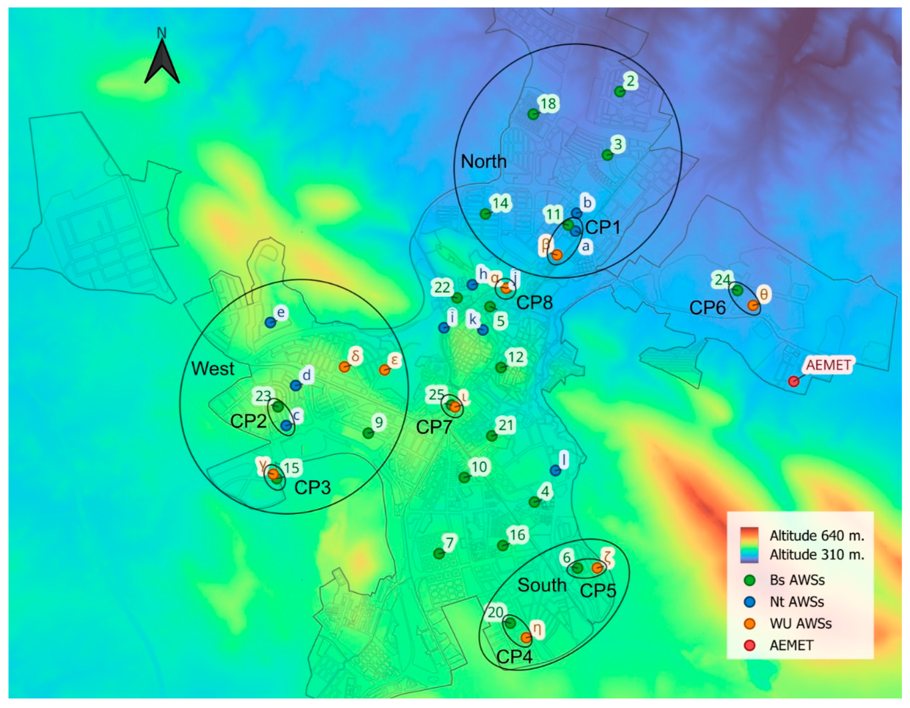
In order to deal with the analysis, eight control points and three control zones are defined (Figure 6). Their complete definition can be found in Appendices B and C. The evolution over time of the data between the different networks in a typical week of hot weather from August 12th to 18th (which also has a greater number of heat registers from the three networks) is then analysed. Similarly, representative indicators for measuring UHI have been defined; they are absolute values for temperature differences, daily values of the mean weekly maximum and minimum temperatures, the weekly average and amplitude. In addition, the calculation of the CDD (in °C·day) is added to quantify the impact of urban heat on the demand for air-conditioning over a period of time (this is calculated through the difference between the hourly data of the AWSs and a reference temperature, in this case 18 °C [97], which accumulate daily and whose impact is calculated over the 24 hours). In addition, to identify the accumulation of solar radiation that manifests itself during the night, the CDD have been broken down into those corresponding to daytime and nighttime periods (from 7 to 21 h and 21 to 7 h, following the mean time of sunset for that week).
Figure 6.
Distribution of Bs, Nt and WU AWSs in control points and zones, on a topographic map of the city of Cáceres [98].
Figure 6.
Distribution of Bs, Nt and WU AWSs in control points and zones, on a topographic map of the city of Cáceres [98].
5.1. Data Quality Control
A data quality control is performed in two stages. The first takes into account the details of the hourly urban climatic databases [99,100], and of the AWSs [101,102]. Successive control processes are then followed:
- Selection of AWSs according to the amount of data, discarding those that do not reach at least 80% (a smaller percentage is considered insufficient to characterize the period).
- Verification of the temperature range for the period in question, which is set from 11 °C to 47 °C (corresponding to ± 6 °C with respect to the absolute minimum and maximum temperatures registered by the city’s AEMET station in the month of August 2024, 17 °C and 41 °C, respectively [103]).
- Checking the consistency of the readings for the same value continuously, fixing as outliers those hourly values repeated over 5 consecutive hours.
- Searching for sudden or significant changes between consecutive time marks, defining as outliers those hourly registers with variations above 12 °C with respect to the previous one (to maintain the stability and relevance of the data, ensuring coherent data and eliminating the infrequent sudden changes that are usually due to extreme phenomena or measuring errors).
- Checking the validity of the continuity of the data in between observations and the average of the remaining AWS, fixing a threshold of 4 standard deviations (guaranteeing the detection of really extreme values, eliminating extremely rare values possibly due to measuring errors or real anomalies, while also minimizing the elimination of legitimate data).
- Checking the daily oscillation in temperatures, eliminating those registers of the days in which the said oscillation is lower than 9 °C (minimum value of thermal oscillation registered by the AEMET in the city in the period in question).
Thus, following the data quality control performed in this first stage, 20 AWSs of Bs with 12144 registers (97.3% of those available) are maintained, as are 10 AWSs of Nt with 6075 registers (97.4 % of the total) and nine AWSs of WU, with 5597 registers (99.7% of the total).
In the second stage of the control, and based on the now clean registers, the similarities of the two sets of data between the networks are evaluated with respect to the following questions:
- The probability distribution and density of the registers from each AWS, according to different temperature ranges (Figure 7): it can be seen that the registers of the AWSs of Bs and WU are uniformly distributed between the different levels, as happens with those of the AEMET, with similar mean values (29.5 ± 0.4 °C in Bs and WU and 29.4 °C in AEMET) and quartiles (first 25.2 ± 0.6 °C and second 34.4 ± 0.6 °C in Bs and WU and 25.2 and 34.5 °C in AEMET). However, those of the Nt show a great heterogeneity (mean 29.5 ± 1.1 °C, first quartile 25.9 ± 1.2 °C and second quartile 34.8 ± 1.9 °C). The differences between the amplitude of data registered in the AWSs of the different networks are similarly worth noting while Bs and WU show 3.7 °C (from 20.1 to 23.8 °C) and 6.7 °C (from 19.7 to 26.4 °C), respectively; Nt registers 8.7 °C (from 18.2 to 26.9 °C). On the other hand, the AWS of the AEMET presents an oscillation of 23.1 °C.
- Hourly differences between the values registered by all the AWSs of each network (Figure 8): Bs and WU have minimums between 0.9 °C and 0.8 °C, and maximums between 7.6 °C and 7.4 °C, respectively; while in Nt, these values are 2.2 °C and 14.0 °C, respectively.
5.2. Control Points
Eight control points are identified (CP1 to CP8) (Appendices B and C), distributed throughout the city, that are used to compare all the networks: on five occasions AWSs of Bs and WU (CP3 to CP7), on one occasion AWSs of Bs and Nt (CP2) and AWSs of Nt and WU (CP8) and, at one of the control points (CP1), three AWSs, one corresponding to each network.
This study uses scatter plots to check the intensity of the existing relation between the data pairs from the AWSs via linear and quality adjustments of the regression obtained from the determination coefficient R² (in general, the closer the R² value is to 1, the stronger the connection between the two variables, allowing the regression model to be trusted with a high level of confidence).
Looking at the results obtained (Figure 9), there is an evident linear relation in general terms between the data pairs. However, it is worth noting that R² between Bs and Nt, in CP1 and CP2 (0.95458 and 0.91868), is notably lower than those obtained in four of the Bs and WU, in CP3 to CP6 (0.98038 ± 0.00857). It should be pointed out that the behaviour of Bs and WU in CP7 (0.93031) is different. When visiting the area, it is possible to see that there is in fact no AWS in that location. Between Nt and WU in CP8, there is a high R² (0.97411), and in this case the distance between the sensors is less than 20 metres.
In CP1, a lower consistency in the data from the AWS of Nt can be appreciated. The pairs between Nt and Bs (R² 0.95458) and Nt and WU (R² 0.94581) present a similar scattering with respect to the cloud of general points. Nevertheless, when the projection of the Bs and WU pairs of data is analysed, the correlation is greater (R² 0.98202) (Figure 10).
5.2.1. Typical Week
In the weekly analysis (Figure 11), in general, it can be seen that the data from the AWSs of Bs and the WU fluctuate in a similar way (practically identical from CP3 to CP6), with hourly mean differences of 0.8 ± 0.8 °C (less than 1 °C in 70 % of the registers) considering the total number of control points of the two networks. However, the values of the AWSs of Nt present an hourly mean difference of 1.8 ± 1.0 °C and 1.7 ± 1.4 °C, respectively, with respect to the AWSs of Bs and WU (less than 1 °C in 27% and 40% and in 38% and 33% greater than 2 °C of the registers, respectively). This difference between the AWSs of Nt and the rest are greater than 12 h and 15 h, even surpassing 6 °C of difference.
The following general conclusions have been obtained from the analysis of the indicators for each of the CP (Table 1):
- Similar amplitude with small deviations with respect to the mean, from 0 °C to ± 1.0 °C.
- Higher daily registers in the Nt AWSs with respect to the rest, with a mean of 1.6 ± 0.4 °C in the minimum and 2.5 ± 0.4 °C in the maximum with respect to the Bs AWSs, and 1.0 ± 0.2 °C and 2.4 ± 0.3.1 °C, respectively, with respect to the WU AWSs. The differences between the values of the WU and Bs AWSs are small (0.6 ± 0.4 °C in the minimums and 1.1 ± 0.8 °C in the maximums).
- Weekly average greater in the Nt AWSs, with a mean of 1.4 ± 0.1 °C and 1.4 ± 1 °C with respect to the Bs and WU AWSs. There is a mean difference of 0.4 ± 0.3 °C in the weekly average of Bs and WU AWSs.
- A greater average of CDD in the Nt AWSs, with respect to the rest, in totals: 15% and 14% more with respect to the Bs and WU AWS; during daylight: 10% and 9%, respectively; and during the night: 27% and 23%, respectively.
5.3. Control Zones
The three selected areas are on the edge of the city: North, West and South (definition in Appendices B and C) and include AWSs from all three networks.
Figure 12 shows a similar hourly general oscillation between the networks in all three zones and between their AWSs during the week in question. In a more specific analysis, the following should be highlighted:
- The superposition of registers between Bs and WU (mostly in the North and South zones).
- The great similarity between the registers of the AWSs of Bs in each of the three zones (means of 1.6 °C and 0.7 °C in West and South).
- The great difference between the values of the AWSs of WU in the West zone (mean of 1.7 °C and maximum of 4.2 °C).
- The lack of continuity in the registers of the AWSs of Nt (some had to be excluded in the data quality control) and large differences between their registers in the West zone (mean of 2.8 °C and maximum of 7.4 °C), especially in the maximums, which were also very high in the North zone (up to 8.8 °C more than Bs and 9.3 °C more than WU, on August 15th at 16:00 h).
From the analysis of the indicators in each of the zones (Table 2), the following general conclusions have been obtained:
- Large absolute differences between the registers of the AWSs of Nt with a mean of 2.6 ± 0.7 °C and maximum of 6.8 ± 0.8 °C. Bs and WU show greater compactness between their AWSs, with a mean of 1 ± 0.4 °C and 1.3 ± 0.9 °C, and a maximum of 3.7 ± 1.4 °C and 4.5 ± 0.4 °C, respectively.
- A similar amplitude (mean of the AWS) between the networks of the West and South zones, while in the North zone the Nt measures 2.9 °C and 3.7 °C more with respect to the Bs and WU, respectively.
- Larger daily maximum and minimum registers in Nt with respect to Bs and WU, with a mean of 1.4 ± 0.3 °C and 1.2 ± 0.1 °C more in the minimums and 2.9 ± 2.9 °C and 3.6 ± 3.4 °C more in the maximums, respectively. Small differences between Bs and WU, of 0.8 ± 1.0 °C in the minimums and 0.5 ± 0.5 °C in the maximums.
- Weekly average larger in Nt with respect to Bs and WU, with 1.1 ± 1.0 °C and 1.2 ± 1.2 °C more on average, respectively. Mean difference of 0.2 ± 0.2 °C between Bs and WU.
- Similar daytime and nighttime totals for CDD in Bs and WU (difference of 2%). Larger values in Nt with respect to Bs and WU, over 6 °C and 8 °C·day, respectively, in the daytime and approximately 10 °C·day at night. This supposes an increase with respect to Bs and WU of 8 ± 8% and 11 ± 12% in the daytime and 23 ± 4% and 21 ± 0% at night, respectively.
- A similar share between daytime and nighttime CDD, with respect to the total, in all three networks, around 68% and 32%.
6. Discussion of Results
This section is devoted to the examination of the implications derived from the previous sections (3, 4 and 5) that may affect the quality of the results obtained when data from different networks are used. Furthermore, the question arises as to whether these issues can be corrected in the analysis process. These issues are of paramount importance concerning the results, as they can lead to significant errors when utilizing the data for the determination and interpretation of UHI effect in a city.
6.1. Concerning the Choice of Components and Programming of the System
The fundamental difference in the selection and programming of each component lies in the flexibility offered by the purpose-built monitoring that can be tailored to specific requirements. This applies to both the AWS (e.g., sensor type , resolution and uncertainty, integration of radiation shielding, power supply system and reduction of consumption (deep sleep mode), sampling periodicity, transmission protocol, clock, data storage capacity, etc.) and the system, utilizing open firmware developed by the user, which fosters enhanced knowledge and control of processes and functions (e.g., alarms, quality control, remote calibration, etc.).
In this context, it is important to highlight the lack of knowledge that exists in CWONs regarding their components, which are developed in closed source software and hardware. This limitation impedes the user's comprehension of the potential constraints that should be considered for subsequent data utilisation. Furthermore, the heterogeneity in the equipment utilised, attributable to divergent AWS models or the absence of auxiliary components (such as radiation shielding or forced ventilation, which are occasionally offered as optional commercially accessories) can result in a lack of homogeneity in the overall analysis. This issue remains uncorrectable even in the event of a final quality control procedure.
All the analysed networks utilise low-cost RTD AWSs, which are deemed suitable for the UHI study regarding their temperature measurement range, in accordance with the recommendations of the WMO. The utilisation of batteries for power supply necessitates their periodic replacement in all instances, a process that can be more intricate and costly depending on the location of the AWSs, as evidenced by the case of the purpose-built monitoring situated far from facades. Conversely, this is not a concern for CWSs installed by citizens in easily accessible domestic locations. While the implementation of solar panels necessitates a higher initial financial outlay, they do offer greater autonomy, though this is contingent on sunlight availability, necessitating support from battery backup in certain instances, as observed with select AWSs offered by WU.
Another salient factor pertains to the data transmission protocol employed. The LoRaWAN protocol boasts certain advantages, including its long range and low power consumption. Moreover, the utilisation of this protocol, in conjunction with the evolution of centralised data processing systems tailored to open technology, facilitates the scalability of the network and the integration of novel functionalities that adapt the infrastructure to emerging requirements. This adaptation extends beyond the characterisation of UHI, encompassing other domains of smart cities, such as mobility, waste management, and so forth. However, this possibility is limited in CWONs to the commercial device offer of the company in question.
It is imperative to acknowledge the significance of cross-quality control in ensuring the integrity of data. This is particularly relevant in the context of purpose-built monitoring systems, where ad hoc ensemble configurations offer the potential to perform joint pre-calibrations. Such measures facilitate the verification of recorded data within a controlled environment, thereby ensuring the reliability of the results. Conversely, cross-quality control, facilitated by centralised CWON systems, necessitates a minimum density of devices deployed in each zone, which was not guaranteed in the case study.
In this section, it is also worth noting that while proprietary networks allow data downloads to be programmed and customised display panels to be designed, CWON are preset to the type of graphical display on the manufacturer's website or mobile application, and only some CWON allow data to be downloaded automatically.
Finally, it should be noted that, in contradistinction, the development and maintenance of these purpose-built monitoring systems necessitates the presence of specialised personnel who possess an advanced understanding of electronics, telecommunications, and sensor technology. Conversely, in the case of CWON, the user is not required to develop these skills as they are incorporated and associated with the initial purchase of the device.
6.2. Concerning the Location and Installation of Measuring Devices
The development of proprietary networks facilitates the generation of dense and uniform networks representing LCZ in accordance with WMO recommendations. In this context, the coordinates and pertinent environmental data for each AWS are meticulously recorded. Conversely, CWON networks characteristically exhibit data shadows within urban areas, particularly in economically disadvantaged regions. Additionally, the recorded coordinates of the AWSs are not always accurate and may, in certain instances, be inaccurate (as discussed in 4.3). The underlying causes of this phenomenon are multifaceted, including, but not limited to, concerns regarding data security, changes in residential address without duly updating the relevant data, and a lack of cooperation from the property owners. This particularity demonstrates scenarios in which there may be a lack of correlation between the data and the measurement point.
It is important to acknowledge the absence of uniformity in the locations of the CWON AWSs on the vertical scale. The height of their placement can vary significantly depending on whether they are situated on low or high floors. This is because they do not respond to the urban canopy or to the roughness of the city. It is also worth noting that the CWONs do not record the aforementioned height or other issues that may reflect micro-scale measurements and, consequently, microclimates that are not representative of the LCZ. These issues cannot be rectified or identified through data quality checks.
6.3. Concerning the Analysis of Measurement Data
The individual quality control conducted on each network revealed a high proportion of valid data across all three networks, thereby enabling their initial and interchangeable use for UHI research. However, in a more advanced quality control analysis, where all devices from the three networks are compared to each other, it has been observed that the distribution of records across different temperature ranges is highly uniform in the proprietary network but significantly variable in the CWON. The maximum difference in recorded amplitudes reaches approximately 9 °C. Additionally, a discrepancy of up to 14 °C has been identified between the hourly records of their AWSs, a value deemed highly improbable for UHIs in any medium-sized city.
Regarding the data analysis conducted at the selected control points and zones of the three networks, significant discrepancies in the local behaviour of the two CWONs have been identified, both in weekly and monthly data. While the WU network exhibits a high degree of internal consistency, demonstrating strong correlation within its own data, the Nt network tends to display higher values, particularly in the upper temperature ranges, with differences exceeding 2 °C. This discrepancy may be attributed to the superior quality of the commercial devices provided by WU.
7. Conclusions
The integration of monitoring technologies is imperative for the enhancement of urban liveability and the identification of UHI. This article undertakes a comprehensive analysis of several low-cost and real-time urban monitoring networks operating within a medium-sized city. It highlights significant variations in network quality and existing limitations among them. This underscores the necessity for more meticulous data analysis, considering the particular characteristics of each monitoring network in climate studies.
Furthermore, the importance of periodic calibrations of networks and data, as well as quality controls to ensure the reliability of records, is emphasised. Nevertheless, this proves to be insufficient in itself, it is imperative to have a precise characterisation of each station, its location, and the surrounding environment and frequent updates of metadata.
In addition, a significant specific objective outlined in the paper has been addressed. It has been provided a comprehensive description of the deployment of the purpose-built monitoring network carried out in the case study, with a view to facilitating its implementation in other study cases. The commitment to open systems, both in terms of hardware and software, enables the system to be modified according to current needs. However, it is important to note that technological advancement can render a system obsolete in a relatively short period, necessitating replacement with more advanced alternatives.
Purpose-built monitoring systems are competitive in multidisciplinary projects of certain temporal duration developed in small or medium-sized cities. The capacity to align with the distinct stipulations inherent in components and systems of discrete projects facilitates the conceptualisation of superior solutions with considerably diminished investment, and monitoring systems that are commensurate with the requirements demanded by each project. However, the necessity for specialised personnel, particularly during deployment and maintenance phases, necessitates the transfer of responsibility to organisations or institutions that can ensure the preservation of these systems. In the case of large cities, where the effects of UHI are more pronounced, the use of existing citizen networks presents a great opportunity, as they do not require deployment and allow the download of historical data without prior studies and implementation. However, the reliance on CWON does not guarantee the persistence of the monitoring system.
The research undertaken has illuminated future lines of research and the challenges that lie ahead, which further extend the existing research trajectory. While the analysis has been primarily focused on UHI, there is potential for the extension of monitoring networks to encompass other critical aspects of Smart Cities, including air quality, noise, mobility, and waste management, among others. These additional factors contribute to the overall well-being of the population. The infrastructure designed in this study is extrapolable and could be implemented in these areas. It is imperative to analyse the network design in a modular and adaptable manner, given the rapid advancements in variable measurement, telecommunications, data processing, and storage, which can shorten the system's lifecycle.
In order to ensure the reliability of citizen devices in research contexts, it is essential that companies incorporate GPS systems to ensure the correct georeferencing of data. Furthermore, the provision of precise information regarding identification, the type of AWS, and the presence of solar protection and ventilation is imperative. Furthermore, the CWON should provide detailed information on the calibration process carried out, if applicable.
Author Contributions
Conceptualization, M.L. and B.M.; methodology, M.L. and B.M.; software, I.T., P.B. and A.M.; validation, M.L. and B.M.; formal analysis, M.L. and B.M.; investigation, M.L. and B.M.; resources, I.T.; data curation, M.L. and B.M.; writing—original draft preparation, M.L. and B.M.; writing—review and editing, M.L. and B.M.; visualization, M.L. and B.M.; supervision, M.L. and B.M.; project administration, M.L. and B.M.; funding acquisition, M.L., B.M. and P.B. All authors have read and agreed to the published version of the manuscript.
Funding
This research was funded by the Junta de Extremadura [Regional Government of Extremadura, the Ministry of Economy, Science and Digital Agenda], and the European Social Fund, through the "Grants for the recruitment of predoctoral research personnel in training within the Extremadura System of Science, Technology, and Innovation” [PD23036].
Data Availability Statement
The authors are able to provide measurement data upon request.
Acknowledgments
The bespoke network implementation was possible through OLADAPT Project: Heat Waves and Cities: Adaptation and Resilience of the Built Environment. Subproject: Continuous monitoring for modeling, simulation and adaptation to heat waves. Programme to Promote Scientific-Technical Research and its Transfer, within the framework of the State Plan for Scientific, Technical and Innovation Research 2021-2023. Ministry of Science, Innovation and Universities, Spain Government, grant number of PID2022-138284OB-C33
Conflicts of Interest
The authors declare no conflicts of interest. The funders had no role in the design of the study; in the collection, analyses, or interpretation of data; in the writing of the manuscript; or in the decision to publish the results.
Abbreviations
The following abbreviations are used in this manuscript:
| ABP | Activation By Personalization |
| ABS | Acrylonitrile Butadiene Styrene |
| API | Application Programming Interface |
| AWS | Automatic Weather Station |
| Bs | Bespoke network |
| CDD | Cooling Degree Days |
| CP | Control Point |
| CPU | Central Processing Unit |
| CWON | Citizen Weather Observer Networks |
| CWS | Citizen Weather Station |
| HTTP | Hypertext Transfer Protocol |
| HUZ | Homogeneus Urban Zone |
| ID | Identification |
| IDE | Integrated Development Environment |
| IoT | Internet of Things |
| IPCC | Intergovernmental Panel on Climate Change |
| ISM bands | Industrial, Scientific and Medical bands |
| LCZ | Local Climate Zones |
| MCU | Microcontroller Unit |
| MQTT | Message Queuing Telemetry Transport |
| NMHS | National Meteorological and Hydrological Services |
| Nt | Netatmo network |
| NTP | Network Time Protocol |
| RF | Radio Frequency |
| RTC | Real-Time Clock |
| RTD | Real-Time Data |
| SNR | Signal-Noise Ratio |
| SQL | Structured Query Language |
| SUHI | Surface Urban Heat Island |
| UCL | Urban Canopy Layer |
| UCZ | Urban Climate Zone |
| UHI | Urban Heat Island |
| USB | Universal Serial Bus |
| VM | Virtual Machine |
| WMO | World Meteorological Organization |
| WU | Weather Underground network |
Appendix A
Stations Compatible with the WU Network.

Table A1.
Features of stations.
| Brand and Model | Physical specifications | Type: parameters (range/ accuracy/ precision) // Sampling rate/Polling rate | CPU functions | Data transmission | Peripheral equipment |
|---|---|---|---|---|---|
| RainWise MK4-C Compact Cellular Weather Station | 28x58x91 cm 4 kg Highly durable materials |
Basic: temperature (Range: - 40 to 60 °C/ Accuracy ± 0.25 °C/ Resolution 0.1 °C), relative humidity (Range: 0 to 100%/ Accuracy ± 1.5% (from 0-80%)/ resolution 1%), precipitation, atmospheric pressure and wind. // Records every 1 minute. Displays every 15 minutes | Factory CPU. Includes factory averaging: Records every minute. The reported value is the average of the 15-minute logs. Highs and lows are based on 1-minute readings. Activation required: Activating Data Plan & Registering Online via their website using the RainWise MK4-C MAC address and serial number. | Data transmission via SIM/LTE connectivity, supporting CAT/LTE-M and NB-IoT cellular networks. Data is sent every 15 minutes. | 1. Solar Panel mono crystaline 7V 2.3 W + Battery Non-Spillable 4V 4.5Ah AGM sealed lead-acid 1A peak, 12 mA typical. Battery Life: 2 to 5 years typical |
| RainWise PWS Direct to Weather Underground | Equivalent characteristics in terms of dimensions, materials and sensors. | Basic: temperature, relative humidity, precipitation, atmospheric pressure, wind, and dew point temperature. No capability to add additional sensors to this station. // Real-time data updates up to 3 seconds |
Based on the same hardware platform as the MK4-C. Preprogrammed WU-100 interface for direct connection to the Weather Underground® personal weather station (PWS) network. Optimized for seamless integration with the WU network | WiFi / Network Interface IP-100: Gateway to the Internet; enables unprecedented transmission and access to real-time weather data through multiple formats. Storage and forwarding capabilities. | Solar-powered with backup battery. |
| Davis VantageVue Package | 33x34x15 cm 3 kg UV-resistant ABS and ASA plastic |
Basic: Temperature (Range: -40 to 65 °C/ Accuracy: ±0.3°C), relative humidity (Range: 0 to 100%/ Accuracy: ±2%), precipitation, atmospheric pressure, and wind. Type: Temperature: Silicon diode with PN junction / Relative humidity: Film capacitor. // Real-time data updates every 2.5 seconds. | Integrated CPU in the WeatherLink Console. It is responsible for receiving, processing, and converting into digital format the signals coming from the external sensors of the Sensor Suite. It also performs internal calculations to generate derived parameters such as heat index, dew point, barometric trends, and weather forecasts, which can then be displayed on the console screen. It acts as the core that manages the WeatherLink Console’s user interface, enabling data visualization through tabs (such as “Current Weather,” “Graph,” “Data,” and “Map”), and facilitating connection to online services for data publishing and storage. Additionally, it handles system settings, including alarms and calibration. |
WiFi. Complemented by devices such as AirBridge or WeatherBridge. | Solar panel (5 watts) + built-in supercapacitor. Backup lithium battery (3-volt CR-123 lithium cell) with a lifespan of 8 months to 2 years. |
| Ambient Weather WS-2902B | 38x28x25.5 cm | Extended: temperature (Range: -40 to 65 °C/ Accuracy ± 2 °C/ Resolution 0.1 °C), relative humidity (Range: 10 to 99% / Accuracy ± 5%/ resolution 1%), precipitation, atmospheric pressure, wind and solar radiation and UV. // Records every 5 minutes | It receives the analog signals from the sensors and converts them into digital data that can be processed. Then, it applies calibration algorithms to correct the measurements. Additionally, it runs the internal software that coordinates the station's operation, controlling aspects such as time synchronization, screen updating, alarm management, and executing calibration and reset functions. | WiFi (Sensor Array RF Frequency: 915 MHz. WiFi Console RF Frequency: 2.4 GHz) |
Solar + supercapacitor. Backup battery (3 AAA batteries) |
| Bloomsky Weather Station | 33x20x18 cm 1 kg |
Extended: temperature (Range: -20 to 55 °C/ Accuracy: ±0.3 °C), relative humidity (Range: 0 to 100%/ Accuracy: ±3% (from 10-90%)), precipitation, atmospheric pressure, wind, UV radiation, and real-time camera. Type: thermometer, hygrometer. // Records every 5 minute | It collects the signals from the various connected sensors and processes them to generate readings of the meteorological variables. Then, it stores data and performs internal calculations to obtain derived parameters, according to what is configured by the user or preset in the firmware. It also manages communication and controls system functions. | WiFi. Weather data and real-time images are transmitted by the built in WiFi module at regular intervals throughout the day. | Solar option. AC & Battery (1 Lithium Ion battery) |
| AcuRite 5-in- 1 Weather Environment System | 35x27.5x14 cm 1.8 kg |
Basic: 5-in-1 sensor: temperature (Range: -40 to 70 °C/ Accuracy: ±1 °C), relative humidity (Range: 1 to 99%), precipitation, atmospheric pressure, and wind. It features an internally powered aspirating fan, powered by a solar panel. // Records every 5 minutes |
Storage of 8760 records. |
WiFi. Communicates via a 433 MHz signal. | Solar + backup batteries (4 AA lithium batteries) (providing up to 12 hours of operation during a power outage) |
| La Crosse Professional Weather Station | 20x15x4 cm 400 gr Durable plastic |
Basic: temperature (Range: -40 to 60 °C/ Accuracy: ±0.5 °C), relative humidity (Range: 10 to 99%), precipitation, atmospheric pressure, and wind. Type: LTV-TH5i sensor (temp and RH) and LTV-WSDR1 sensor (others). // Records every 5 minute | - | WiFi. Frecuencia de transmisión: 915 MHz | Solar and Battery Powered (LTV-TH5i sensor: 2 AA alkaline batteries and LTV-WSDR1: 3 AA alkaline batteries). Battery life: 2 years. |
| Netatmo Weather Station | Indoor module: 45x45x155 mm Outdoor module: 45x45x105 mm Anodized aluminum |
Light: indoor temperature (Range: 0 to 50 °C/ Accuracy: ±0.3 °C), outdoor temperature (Range: -40 to 65 °C / Accuracy: ±0.3 °C), relative humidity (Range: 0% to 100% / Accuracy: ±3%), barometric pressure, CO₂. // Records every 5 minutes |
Data processing: receives measurements from the integrated sensors and processes them to generate understandable data. Communication management: controls the transmission of data between modules and ensures connection to the home Wi-Fi network to send information to Netatmo's servers. Temporary storage: maintains temporary records of the measurements before transmission, ensuring data integrity in case of connection interruptions. | Data transmission between accessory modules and the main module is done via a low-power wireless connection. Data transmission to the Netatmo server: Wi-Fi – The main module connects to the home Wi-Fi network using the 2.4 GHz band. The station is not compatible with networks operating exclusively on the 5 GHz band. |
Indoor module: USB power adapter. Outdoor module: 2 AAA batteries, with a lifespan of up to 2 years. |
Appendix B
Characterization of control points and study zones.
Table B1.
Characterization of control points.
| Control points | (% records) | Distance between AWSs (m) | District | ||
|---|---|---|---|---|---|
| AWS Bs | AWS Nt | AWS WU | |||
| CP1 | 11 (100%) | a (81%) | β (100%) | 100/300 | Mejostilla / San Jorge |
| CP2 | 23 (100%) | c (100%) | - | 250 | Los Castellanos |
| CP3 | 15 (100%) | - | γ (100%) | 60 | Junquillo |
| CP4 | 20 (98%) | - | η (100%) | 215 | Casaplata |
| CP5 | 6 (89%) | - | ζ (100%) | 200 | Vistahermosa |
| CP6 | 24 (100%) | - | θ (100%) | 250 | Campus universitario |
| CP7 | 25 (100%) | - | ι (99%) | 40 | Cánovas |
| CP8 | - | j (100%) | α (100%) | 20 | Infanta Isabel |
Table B2.
Characterization of control zones.
| North zone | West zone | South zone | |
|---|---|---|---|
| Elevation (Altitude) (m) |
40 (from 350 to 390) |
35 (from 350 to 385) |
25 (from 440 to 465) |
| Extension (Ha) | 294 | 176 | 77 |
| District | Cáceres el Viejo, Montesol, Mejostilla, Gredos and San Jorge |
El Junquillo, La Sierrilla, Los Castellanos and Cabezarrubia |
Vistahermosa and Casa Plata |
| Open areas or green zones | No large wooded areas on non-urban edges and no green areas within neighbourhoods |
Large green areas nearby both on non-urban edges and in the inner urban area | Unbuilt urbanized areas, with extensive surrounding crop areas |
| HUZ | Terraced and row houses and Semi-Open Collective (from 1 to 4 floors high) | ||
| Construction date | 1995 - 2010 | 1995 - 2010 | 2002 - present |
| Number of AWSs (Bs / Nt / WU) | 8 units (2, 3, 11, 14, 18 / a, b / β) |
9 units (9, 15, 23 / c, d, e / γ, δ, ε) |
4 units (6, 20 / ζ, η) |
| % records | 99% | 100% | 99% |
Appendix C
Location of control points and study zones:
Figure C1.
Control point CP1 in the North zone.
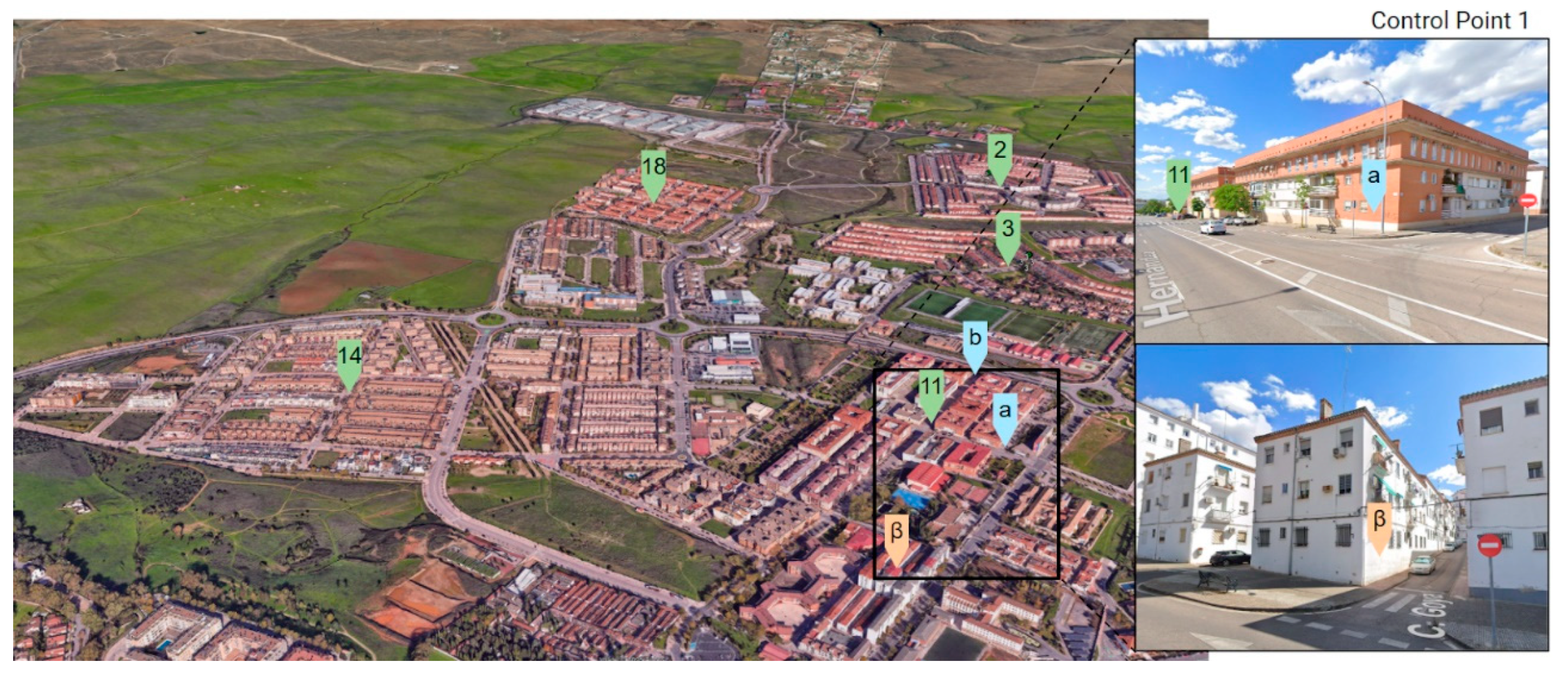
Figure C2.
Control point CP2 and CP3 in the West zone.
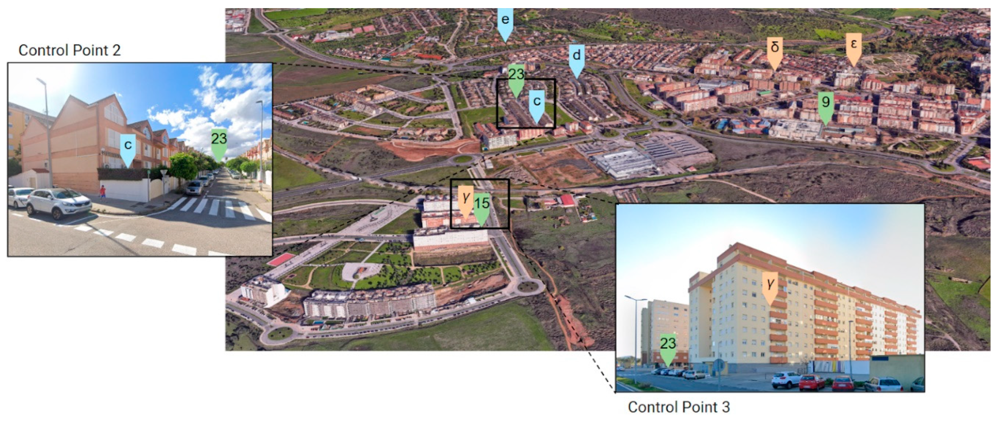
Figure C3.
Control point CP4 and CP5 in the South zone.
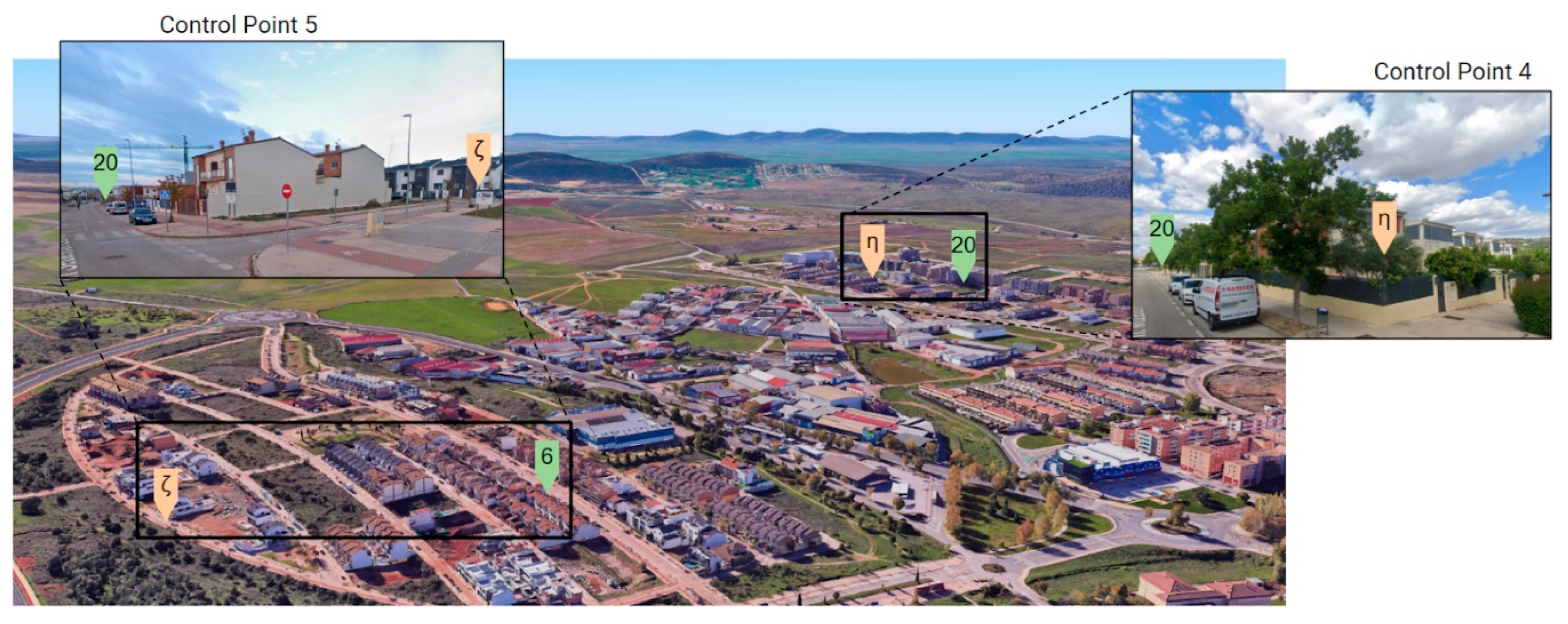
Figure C4.
Control point CP6 (East).
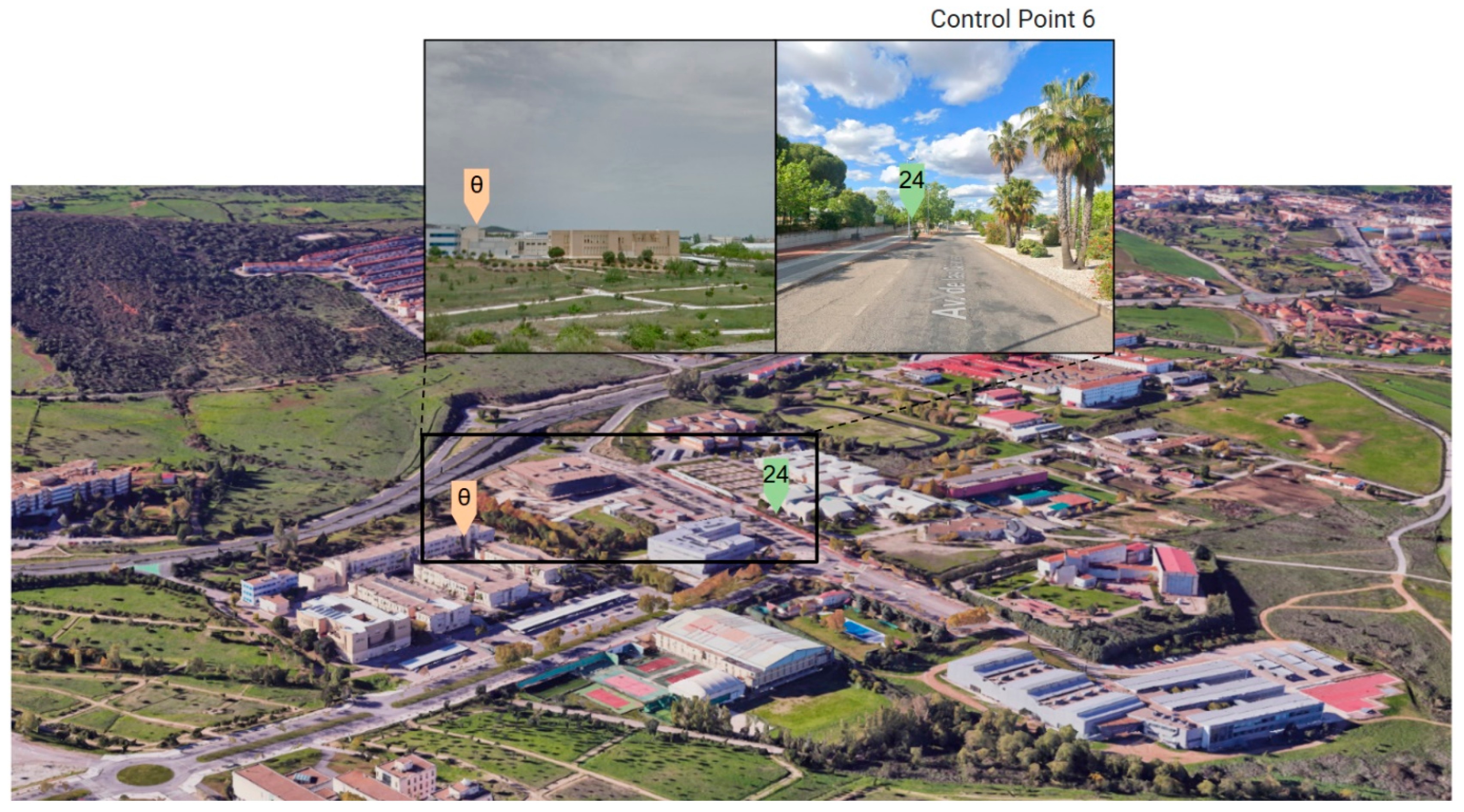
Figure C5.
Control point CP7 (Center).
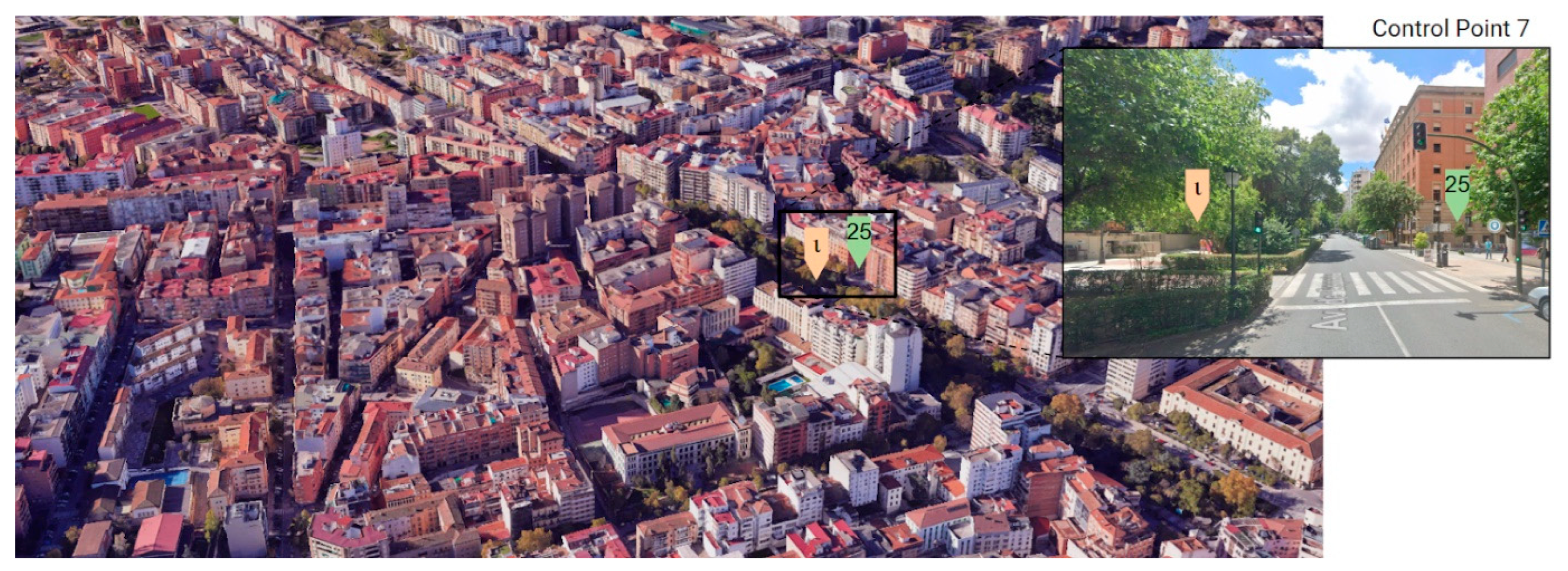
Figure C6.
Control point CP8 (Center).
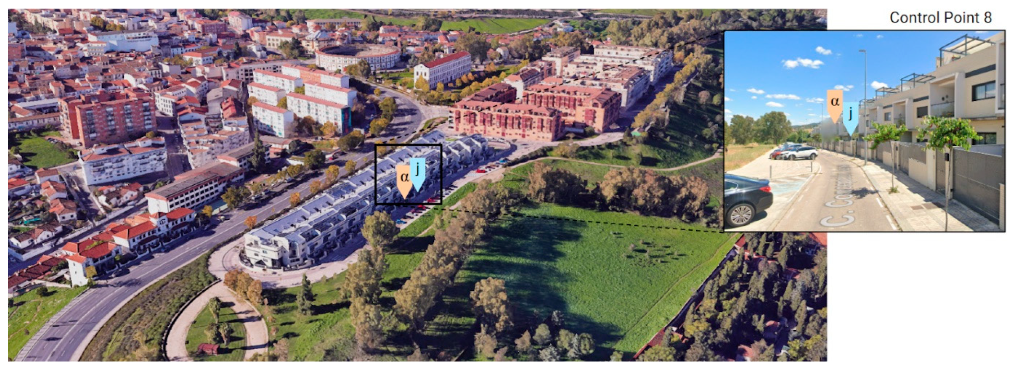
References
- United Nations, Department of Economic and Social Affairs, Population Division, World Urbanization Prospects. The 2018 Revision, New York, 2018.
- UN-Habitat, European Commission, Healthier Cities and Communities Through Public Spaces, 2025.
- Olaniyi, O.J. Okunleye, S.O. Olabanji, Advancing Data-Driven Decision-Making in Smart Cities through Big Data Analytics: A Comprehensive Review of Existing Literature, Current Journal of Applied Science and Technology 42 (2023) 10–18. [CrossRef]
- Open & Agile Smart Cities, Open & Agile Smart Cities & Communities (OASC), (2025). https://oascities.org/ (accessed , 2025). 10 April.
- Centre for Urban Transformation, G20 Global Smart Cities Alliance, (2025). https://www.globalsmartcitiesalliance.org/home (accessed , 2025). 10 April.
- Organisation for Economic Co-operation and Development, Organisation for Economic Co-operation and Development (OECD), (2025). https://www.oecd.org/en/about/programmes/the-oecd-programme-on-smart-cities-and-inclusive-growth0.html (accessed , 2025). 10 April.
- Governance of the Living-in.EU Community (Go Li.EU), Smart Communities Network, (2025). https://living-in.eu/eu-support-services/smart-communities-network (accessed , 2025). 10 April.
- D. Müller-Eie, I. D. Müller-Eie, I. Kosmidis, Sustainable mobility in smart cities: a document study of mobility initiatives of mid-sized Nordic smart cities, European Transport Research Review 15 (2023) 36. [CrossRef]
- D. Szpilko, A. D. Szpilko, A. de la Torre Gallegos, F. Jimenez Naharro, A. Rzepka, A. Remiszewska, Waste Management in the Smart City: Current Practices and Future Directions, Resources 12 (2023) 115. [CrossRef]
- Z. Mohammadzadeh, H.R. Z. Mohammadzadeh, H.R. Saeidnia, A. Lotfata, M. Hassanzadeh, N. Ghiasi, Smart city healthcare delivery innovations: a systematic review of essential technologies and indicators for developing nations, BMC Health Serv Res 23 (2023) 1180. [CrossRef]
- S.L. Ullo, G.R. S.L. Ullo, G.R. Sinha, Advances in Smart Environment Monitoring Systems Using IoT and Sensors, Sensors 20 (2020) 3113. [CrossRef]
- A. Faraji, M. A. Faraji, M. Rashidi, F. Rezaei, P. Rahnamayiezekavat, A Meta-Synthesis Review of Occupant Comfort Assessment in Buildings (2002–2022), Sustainability 15 (2023) 4303. [CrossRef]
- Biennial of Public Space, United Nations Programme on Human Settlements (UN-Habitat), Charter of Public Space, (2016).
- The Intergovernmental Panel on Climate Change (IPCC), The Intergovernmental Panel on Climate Change (IPCC), (2025). https://www.ipcc.ch/ (accessed , 2025). 10 April.
- H. Afaq, D.N. H. Afaq, D.N. Chambers, T.R. Zolnikov, Urban Heat Islands. The Palgrave Encyclopedia of Urban and Regional Futures, in: The Palgrave Encyclopedia of Urban and Regional Futures, Springer International Publishing, Cham, 2022: pp. 1–7. [CrossRef]
- Md. Nuruzzaman, Urban Heat Island: Causes, Effects and Mitigation Measures - A Review, International Journal of Environmental Monitoring and Analysis 3 (2015) 67. [CrossRef]
- L. Mentaschi, G. L. Mentaschi, G. Duveiller, G. Zulian, C. Corbane, M. Pesaresi, J. Maes, A. Stocchino, L. Feyen, Global long-term mapping of surface temperature shows intensified intra-city urban heat island extremes, Global Environmental Change 72 (2022) 102441. [CrossRef]
- A. Wandl, F. A. Wandl, F. van der Hoeven, Amsterwarm: Mapping the landuse, health and energy-efficiency implications of the Amsterdam urban heat island, Building Services Engineering Research and Technology 36 (2015) 67–88. [CrossRef]
- L. Echevarría Icaza, F.D. L. Echevarría Icaza, F.D. van der Hoeven, A. van den Dobbelsteen, The Urban Heat Island Effect in Dutch City Centres: Identifying Relevant Indicators and First Explorations, in: 2016: pp. 123–160. [CrossRef]
- K.I. Morris, S. K.I. Morris, S. Aekbal Salleh, A. Chan, M.C.G. Ooi, Y.A. Abakr, M.Y. Oozeer, M. Duda, Computational study of urban heat island of Putrajaya, Malaysia, Sustain Cities Soc 19 (2015) 359–372. [CrossRef]
- P. Ichim, L. P. Ichim, L. Sfîcă, A. Kadhim-Abid, Characteristics of Nocturnal Urban Heat Island of Iaşi During a Summer Heat Wave (1-6 of 17), in: 2018: pp. 253–260. 20 August. [CrossRef]
- G.A. Garau, J.L. G.A. Garau, J.L. Garau, The urban heat island in Palma (Majorca, Balearic islands): Progress in the study of urban climate in a Mediterranean coastal city, Boletin de La Asociacion de Geografos Espanoles 2018 (2018) 392–418. [CrossRef]
- World Meteorological Organization, WMO, n.d. https://wmo.int/es (accessed , 2025). 10 April.
- World Meteorological Organization (WMO), Guide to Instruments and Methods of Observation (Volume I - Measurement of Meteorological Variables, Volume II - Measurement of cryospheric variables, Volume III - Observing Systems, Volume IV - Space-based Observations and Volume V - Quality Assurance and Management of Observing Systems), 2023 edition, Geneva, Switzerland, 2023.
- S. Peng, S. S. Peng, S. Piao, P. Ciais, P. Friedlingstein, C. Ottle, F.-M. Bréon, H. Nan, L. Zhou, R.B. Myneni, Surface Urban Heat Island Across 419 Global Big Cities, Environ Sci Technol 46 (2012) 696–703. [CrossRef]
- MODIS Moderate Resolution Imaging Spectoradiometer, (n.d.). https://modis.gsfc.nasa.gov/ (accessed , 2025). 10 April.
- NASA/USGS, Landsat Science, (2025). https://landsat.gsfc.nasa.gov/ (accessed , 2025). 10 April.
- Agencia Espacial Europea, Sentinel, (2025). https://sentinels.copernicus.eu/ (accessed , 2025). 10 April.
- Q. Weng, Thermal infrared remote sensing for urban climate and environmental studies: Methods, applications, and trends, ISPRS Journal of Photogrammetry and Remote Sensing 64 (2009) 335–344. [CrossRef]
- L. Ma, X. L. Ma, X. Zhu, C. Qiu, T. Blaschke, M. Li, Advances of Local Climate Zone Mapping and Its Practice Using Object-Based Image Analysis, Atmosphere (Basel) 12 (2021) 1146. [CrossRef]
- C. Wang, X. C. Wang, X. Bi, Q. Luan, Z. Li, Estimation of Daily and Instantaneous Near-Surface Air Temperature from MODIS Data Using Machine Learning Methods in the Jingjinji Area of China, Remote Sens (Basel) 14 (2022) 1916. [CrossRef]
- Steinbeis Europa Zentrum, Smart Cities Marketplace, (2025). https://www.steinbeis-europa.de/en/projects/smart-cites-marketplace-2-0 (accessed , 2025). 10 April.
- EURO CITIES, Smart Cities Information System, (2025). https://eurocities.eu/projects/smart-cities-information-system/ (accessed , 2025). 10 April.
- Eumetnet, Eumetnet, (2025). https://www.eumetnet.eu/ (accessed , 2025). 10 April.
- C. Hahn, I. C. Hahn, I. Garcia-Marti, J. Sugier, F. Emsley, A.-L. Beaulant, L. Oram, E. Strandberg, E. Lindgren, M. Sunter, F. Ziska, Observations from Personal Weather Stations—EUMETNET Interests and Experience, Climate 10 (2022) 192. [CrossRef]
- V.R. Golroudbary, Y. V.R. Golroudbary, Y. Zeng, C.M. Mannaerts, Z. Su, Urban impacts on air temperature and precipitation over the netherlands, Clim Res 75 (2018) 95–109. [CrossRef]
- L. Chapman, C. L. Chapman, C. Bell, S. Bell, Can the crowdsourcing data paradigm take atmospheric science to a new level? A case study of the urban heat island of London quantified using Netatmo weather stations, International Journal of Climatology 37 (2017) 3597–3605. [CrossRef]
- F. Meier, D. F. Meier, D. Fenner, T. Grassmann, M. Otto, D. Scherer, Crowdsourcing air temperature from citizen weather stations for urban climate research, Urban Clim 19 (2017) 170–191. [CrossRef]
- M. Feichtinger, R. M. Feichtinger, R. de Wit, G. Goldenits, T. Kolejka, B. Hollósi, M. Žuvela-Aloise, J. Feigl, Case-study of neighborhood-scale summertime urban air temperature for the City of Vienna using crowd-sourced data, Urban Clim 32 (2020) 100597. [CrossRef]
- L.W. de Vos, A.M. L.W. de Vos, A.M. Droste, M.J. Zander, A. Overeem, H. Leijnse, B.G. Heusinkveld, G.J. Steeneveld, R. Uijlenhoet, Hydrometeorological Monitoring Using Opportunistic Sensing Networks in the Amsterdam Metropolitan Area, Bull Am Meteorol Soc 101 (2020) E167–E185. [CrossRef]
- A. Napoly, T. A. Napoly, T. Grassmann, F. Meier, D. Fenner, Development and Application of a Statistically-Based Quality Control for Crowdsourced Air Temperature Data, Front Earth Sci (Lausanne) 6 (2018). [CrossRef]
- C.-Y. Sun, S. C.-Y. Sun, S. Kato, Z. Gou, Application of Low-Cost Sensors for Urban Heat Island Assessment: A Case Study in Taiwan, Sustainability 11 (2019) 2759. [CrossRef]
- A. Martinez-Soto, M. A. Martinez-Soto, M. Vera-Fonseca, P. Valenzuela-Toledo, A. Melillan-Raguileo, M. Shupler, Heat on the Move: Contrasting Mobile and Fixed Insights into Temuco’s Urban Heat Islands, Sensors 25 (2025) 1251. [CrossRef]
- G. Battista, L. G. Battista, L. Evangelisti, C. Guattari, E. De Cristo, R. De Lieto Vollaro, F. Asdrubali, An Extensive Study of the Urban Heat Island Phenomenon in Rome, Italy: Implications for Building Energy Performance Through Data from Multiple Meteorological Stations, International Journal of Sustainable Development and Planning 18 (2023) 3357–3362. [CrossRef]
- E. Husni, G.A. E. Husni, G.A. Prayoga, J.D. Tamba, Y. Retnowati, F.I. Fauzandi, R. Yusuf, B.N. Yahya, Microclimate investigation of vehicular traffic on the urban heat island through IoT-Based device, Heliyon 8 (2022) e11739. [CrossRef]
- D. Ma, O. D. Ma, O. Brousse, M. De Jode, A. Hudson-Smith, Using Bespoke LoRaWAN Heat Sensors to Explore Microclimate Effects within the London Urban Heat Islands-A Pilot Study in East London, (2024). [CrossRef]
- L. Chapman, C.L. L. Chapman, C.L. Muller, D.T. Young, E.L. Warren, C.S.B. Grimmond, X.-M. Cai, E.J.S. Ferranti, The Birmingham Urban Climate Laboratory: An Open Meteorological Test Bed and Challenges of the Smart City, Bull Am Meteorol Soc 96 (2015) 1545–1560. [CrossRef]
- A. Martín-Garín, J.A. A. Martín-Garín, J.A. Millán-García, R.J. Hernández-Minguillón, M.M. Prieto, N. Alilat, A. Baïri, Open-Source Framework Based on LoRaWAN IoT Technology for Building Monitoring and Its Integration into BIM Models, in: Handbook of Smart Materials, Technologies, and Devices, Springer International Publishing, Cham, 2022: pp. 257–283. [CrossRef]
- M. Ma, E. M. Ma, E. Bartocci, E. Lifland, J.A. Stankovic, L. Feng, A Novel Spatial–Temporal Specification-Based Monitoring System for Smart Cities, IEEE Internet Things J 8 (2021) 11793–11806. [CrossRef]
- S. Bell, D. S. Bell, D. Cornford, L. Bastin, How good are citizen weather stations? Addressing a biased opinion, Weather 70 (2015) 75–84. [CrossRef]
- T.E. Oke, Initial guidance to obtain representative meteorological observations at urban sites, (2006).
- Instituto Nacional de Estadística (INE), Cifras oficiales de población de los municipios españoles en aplicación de la Ley de Bases del Régimen Local (Art. 17), (2025). https://www.ine.es/jaxiT3/Datos.htm?t=2863 (accessed , 2025). 10 April.
- C. Sánchez-Guevara, L. C. Sánchez-Guevara, L. Garmendia Arrieta, B. Montalbán Pozas, OLADAPT: Olas de calor y ciudades: adaptación y resiliencia del entorno construido, Ministerio de Ciencia, Innovación y Universidades PID2022-138284OA-C32 (2023).
- Netatmo, Netatmo Weather, (2025). https://www.netatmo.com/weather-with-netatmo (accessed , 2025). 10 April.
- J. Coney, B. J. Coney, B. Pickering, D. Dufton, M. Lukach, B. Brooks, R.R. Neely, How useful are crowdsourced air temperature observations? An assessment of Netatmo stations and quality control schemes over the United Kingdom, Meteorological Applications 29 (2022). [CrossRef]
- The Weather Company, Weather Underground, (2025). https://www.wunderground.com/ (accessed , 2025). 10 April.
- Meteoclimatic, Meteoclimatic, (2025). https://www.meteoclimatic.net/mapinfo/ESEXT?screen_width=2560 (accessed , 2025). 10 April.
- Noromet, Noromet Asociación Meteorológica del Noroeste Peninsular, (2025). https://noromet.org/ (accessed , 2025). 10 April.
- NCEI National Centers for Environmental Information, NCEI National Centers for Environmental Information, (2025). https://www.ncei.noaa.gov/ (accessed , 2025). 10 April.
- Organización Meteorológica Mundial, Guía de Instrumentos y Métodos de Observación Meteorológicos, 2014. www.wmo.int.
- F.A. Sánchez-Sánchez, M. F.A. Sánchez-Sánchez, M. Vega-De-Lille, A.A. Castillo-Atoche, J.T. López-Maldonado, M. Cruz-Fernandez, E. Camacho-Pérez, J. Rodríguez-Reséndiz, Geo-Sensing-Based Analysis of Urban Heat Island in the Metropolitan Area of Merida, Mexico, Sensors 24 (2024) 6289. [CrossRef]
- A. Mathew, T.H. A. Mathew, T.H. Aljohani, P.R. Shekar, K.S. Arunab, A.K. Sharma, M.F.M. Ahmed, U.I.A. Idris, H. Almohamad, H.G. Abdo, Spatiotemporal dynamics of urban heat island effect and air pollution in Bengaluru and Hyderabad: implications for sustainable urban development, Discover Sustainability 6 (2025). [CrossRef]
- iRay Electronic Engineering, iRay Electronic Engineering, (2025). https://ray-ie.com/ (accessed , 2025). 10 April.
- T.S.C. Sensirion, Datasheet SHT3x-DIS, (2022). www.sensirion.com.
- GitHub, MCU ATMega328P, (2025). https://github.com/raymirabel/LoRaTH (accessed , 2025). 10 April.
- DigiKey, 2J0C15-868-C885G 868 MHz ISM Connector Mount, DigiKey (2025). https://www.digikey.es/es/products/detail/2j-antennas/2J0C15-868-C885G/22108775?srsltid=AfmBOorQJKnMrtUYXOKnezqCeCbtP6lyFCDOWMEuLBIVJtCs9TXUghbo (accessed , 2025). 10 April.
- ETSI, EN 300 220-2 - V3. 2.1 - Short Range Devices (SRD) operating in the frequency range 25 MHz to 1 000 MHz; Part 2: Harmonised Standard for access to radio spectrum for non specific radio equipment, 2018. [Google Scholar]
- ChirpStack, ChirpStack, servidor de red LoRaWAN, (2025). https://www.chirpstack.Io/ (accessed , 2025). 10 April.
- BricoGeek, Adafruit RFM95W LoRa Radio (900 Mhz), (2025). https://tienda.bricogeek.com/lora/1097-adafruit-rfm95w-lora-radio-900-mhz.html (accessed , 2025). 10 April.
- LoRa Alliance®, The Things Network, (2025). https://www.thethingsnetwork.org/docs/lorawan/regional-parameters/eu868/ (accessed , 2025). 10 April.
- JEDEC. Global Standards for the Microelectronics Industry, Standards & Documents, (2025). https://www.jedec.org/document_search?search_api_views_fulltext=JESD47 (accessed , 2025). 10 April.
- RIKA Sensor, RK95-01 Protector solar multiplaca, (2025). https://www.rikasensor.com/rk95-01-multi-plate-ambient-weather-radiation-shield.html (accessed , 2025). 10 April.
- RAK, Outdoor Enclosure for WisGate Developer Gateway, (2025). https://store.rakwireless.com/products/outdoor-enclosure-kit-h?srsltid=AfmBOopTK3Lstjr8Z-xBoMTZYVVnQFxFDnaLxYDzX9DsJZ87mqOEmvyy&variant=37912840634566 (accessed , 2025). 10 April.
- Maker Store, RAK Wireless 7248C WisGate Developer D4H+ (con LTE), (2025). https://maker-store.es/iot-lora-nb-iot-rfid-m2m-co/lora/lora-gateways/7058/rak-wireless-7248c-wisgate-developer-d4h-con-lte (accessed , 2025). 10 April.
- S-Connect, Antenna ISM/LoRA Barracuda OMB.868.B08F21 868MHz 8dBi Omnidirectional Outdoor Wall/Pole Mount N-Type(F), (2025). https://s-connect.es/Antenna-ISM-LoRA-Barracuda-OMB.868.B08F21-868MHz-8dBi-Omnidirectional-Outdoor-Wall-Pole-Mount-N-Type-F/OMB.868.B08F21 (accessed , 2025). 10 April.
- Telegram, Telegram, (2025). https://telegram.org/ (accessed , 2025). 10 April.
- Grafana Labs, Grafana, (2025). https://grafana.com/ (accessed , 2025). 10 April.
- Weather Underground, Personal Weather Station Buying Guide, (2025). https://www.wunderground.com/pws/buying-guide (accessed , 2025). 10 April.
- Netatmo, Avec la Station Météo Intelligente, mesurez précisément votre environnement, (2025). https://www.netatmo.com/fr-fr/smart-weather-station (accessed , 2025). 10 April.
- Netatmo, Weather Guide, (2025). https://www.netatmo.com/es-es/weather-guide/ (accessed , 2025). 10 April.
- Netatmo, Estación meteorológica Netatmo: Análisis completo., (2025). https://estaciondemeteorologia.com/estacion-meteorologica-netatmo/ (accessed , 2025). 10 April.
- Weather Underground, Personal Weather Station Network, (2025). https://www.wunderground.com/pws/about (accessed , 2025). 10 April.
- Mideycontrola.com, Estaciones Meteorológicas, (2025). https://mideycontrola.com/estaciones-meteorologicas (accessed , 2025). 10 April.
- AcuRite, AcuRite Iris (5-in-1) Weather Station, (2025). https://www.acurite.com/collections/iris/products/acurite-iris-5-in-1-weather-station-with-wi-fi-connection-to-weather-underground (accessed , 2025). 10 April.
- Netatmo, Weather API Documentation, (2025). https://dev.netatmo.com/apidocumentation/weather (accessed , 2025). 10 April.
- Netatmo, MeatherMap Netatmo, (2025). https://weathermap.netatmo.com/ (accessed , 2025). 10 April.
- Ambient Weather AirBridge for Davis Weather Stations Quick Start Guide, 2014. www.MeteoBridge.com.
- Ambient Weather, AirBridge Download Center, (2025). https://ambientweather.com/faqs/question/view/id/2477/ (accessed , 2025). 10 April.
- Ambient Weather, The WeatherBridge, (2025). https://ambientweather.com/blog/weatherbridge-easily-connect-davis-acurite-fine-offset-tempest-station-ambientweather (accessed , 2025). 10 April.
- Weather Underground, WunderMap, (2025). https://www.wunderground.com/wundermap (accessed , 2025). 10 April.
- Weather Underground, Weather apps, (2025). https://www.wunderground.com/download (accessed , 2025). 10 April.
- A.G. Davenport, Rationale for determining design wind velocities, 1960.
- Radio Mobile, Radio Mobile - Software de simulación de propagación de RF, (2025). http://radiomobile.pe1mew.nl/ (accessed , 2025). 10 April.
- MeteoEstacion - Estaciones Meteorológicas & Meteorología, Consejos y recomendaciones en la instalación de estaciones meteorológicas para lograr datos de calidad., (2025). https://estaciondemeteorologia.com/recomendaciones-instalacion-estaciones-meteorologicas-datos-calidad/ (accessed , 2025). 10 April.
- Weather Underground, Installing your Personal Weather Station, (2025). https://www.wunderground.com/pws/installation-guide (accessed , 2025). 10 April.
- Ministerio para la Transición Ecológica y el Reto Demográfico, AEMET. Agencia Estatal de Meteorología, (2025). https://www.aemet.es/es/portada (accessed , 2025). 10 April.
- American National Standards Institute, ANSI/ASHRAE Standard 55-2020. Thermal Environmental Conditions for Human Occupancy, 2020.
- Topographic-map.com, Mapa topográfico Cáceres, (2025). https://es-es.topographic-map.com/map-6943l/C%C3%A1ceres/?center=39.46993%2C-6.39462&zoom=15&popup=39.46407%2C-6.39896 (accessed , 2025). 10 April.
- S. Barrao, R. S. Barrao, R. Serrano-Notivoli, J.M. Cuadrat, E. Tejedor, M.A. Saz Sánchez, Characterization of the UHI in Zaragoza (Spain) using a quality-controlled hourly sensor-based urban climate network, Urban Clim 44 (2022) 101207. [CrossRef]
- C. Beck, A. C. Beck, A. Straub, S. Breitner, J. Cyrys, A. Philipp, J. Rathmann, A. Schneider, K. Wolf, J. Jacobeit, Air temperature characteristics of local climate zones in the Augsburg urban area (Bavaria, southern Germany) under varying synoptic conditions, Urban Clim 25 (2018) 152–166. [CrossRef]
- D. Fenner, B. D. Fenner, B. Bechtel, M. Demuzere, J. Kittner, F. Meier, CrowdQC+—A Quality-Control for Crowdsourced Air-Temperature Observations Enabling World-Wide Urban Climate Applications, Front Environ Sci 9 (2021). [CrossRef]
- D. Castro Medina, Mc. D. Castro Medina, Mc. Guerrero Delgado, J. Sánchez Ramos, T. Palomo Amores, L. Romero Rodríguez, S. Álvarez Domínguez, Empowering urban climate resilience and adaptation: Crowdsourcing weather citizen stations-enhanced temperature prediction, Sustain Cities Soc 101 (2024) 105208. [CrossRef]
- AEMET. Agencia Estatal de Meteorología, Analisis estacional. Cáceres, (2025). https://www.aemet.es/es/serviciosclimaticos/vigilancia_clima/analisis_estacional?w=2&l=3469A&datos=temp (accessed , 2025). 10 April.
Figure 1.
Diagram of the Bs information system architecture, including AWSs and the centralized processing system for network data.
Figure 1.
Diagram of the Bs information system architecture, including AWSs and the centralized processing system for network data.
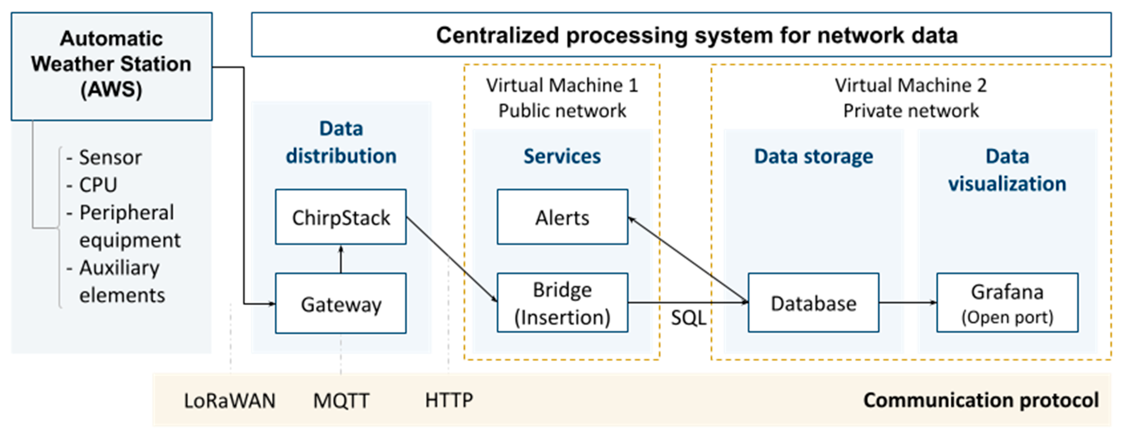
Figure 2.
(a) Typical tolerance of RH over T for SHT35; (b) Appearance of the AWS; (c) Inside the MCU box.
Figure 2.
(a) Typical tolerance of RH over T for SHT35; (b) Appearance of the AWS; (c) Inside the MCU box.
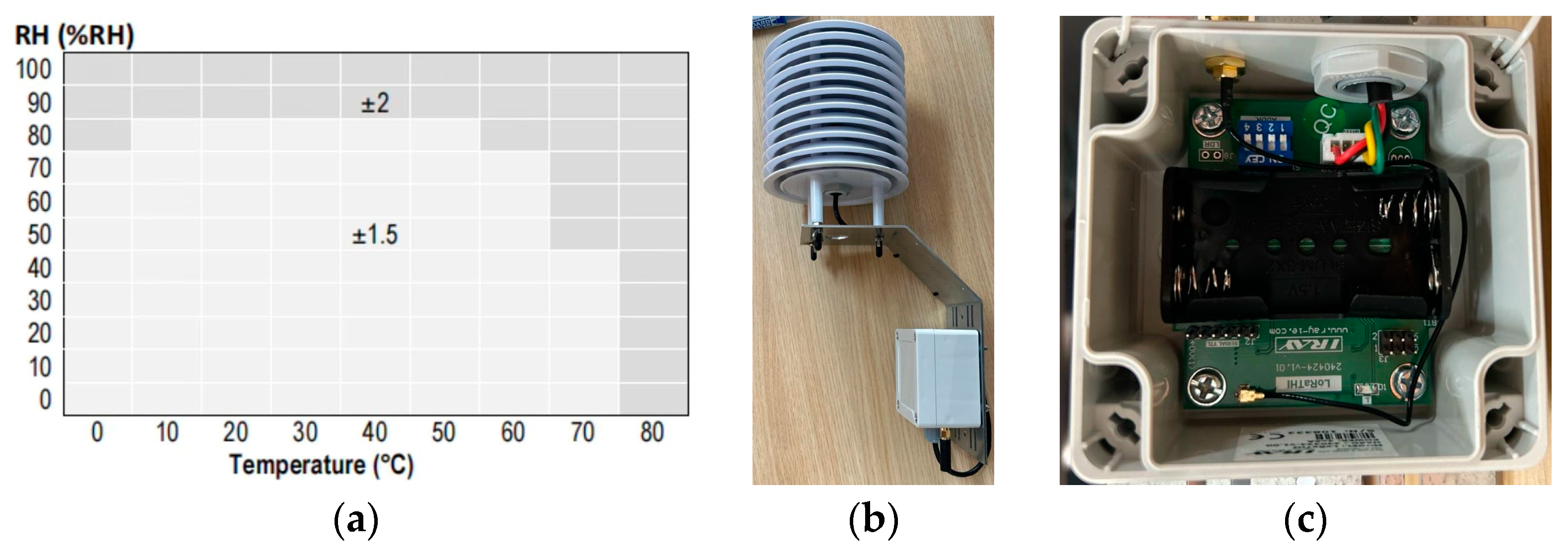
Figure 3.
(a) Characteristics of the communication device antenna; (b) Appearance of the communication device; (c) Inside the waterproof box.
Figure 3.
(a) Characteristics of the communication device antenna; (b) Appearance of the communication device; (c) Inside the waterproof box.
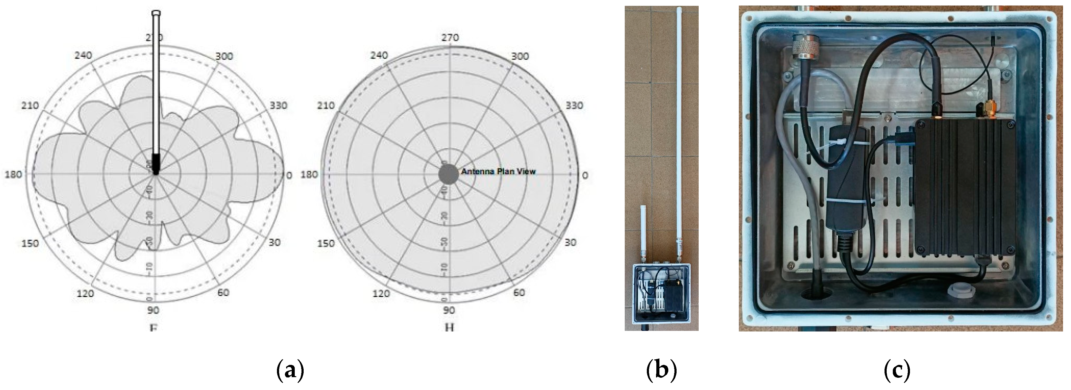
Figure 4.
Location of the AWSs in the neighborhoods of the city of Cáceres according to roughness class and zH and HUZ.
Figure 4.
Location of the AWSs in the neighborhoods of the city of Cáceres according to roughness class and zH and HUZ.
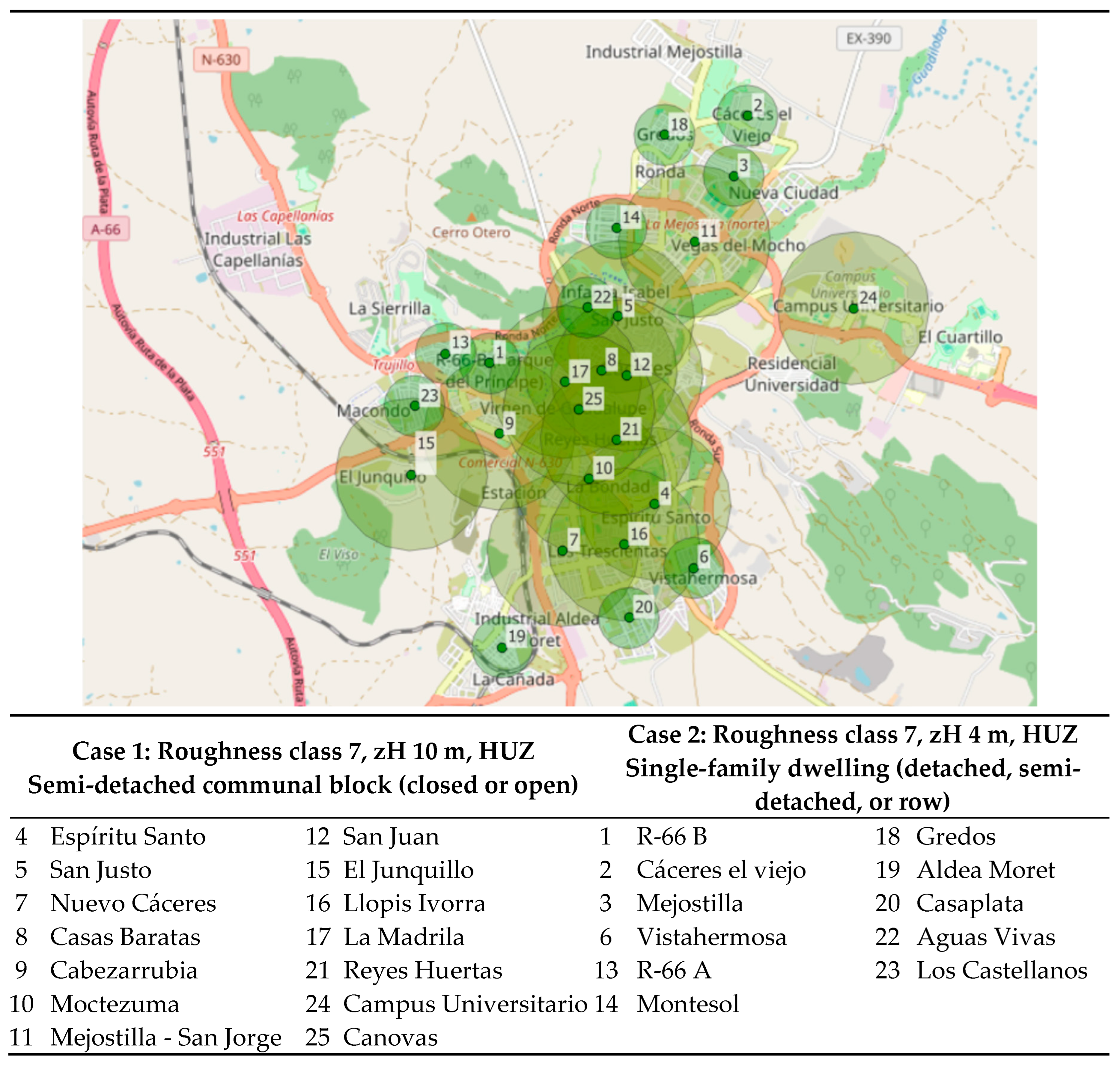
Figure 5.
Correspondence and coverage available between the communication device antennas and AWSs, in Cáceres, with star topology and from 865.0 MHz to 871.0 MHz (number in colour red indicate unaccepted values).
Figure 5.
Correspondence and coverage available between the communication device antennas and AWSs, in Cáceres, with star topology and from 865.0 MHz to 871.0 MHz (number in colour red indicate unaccepted values).
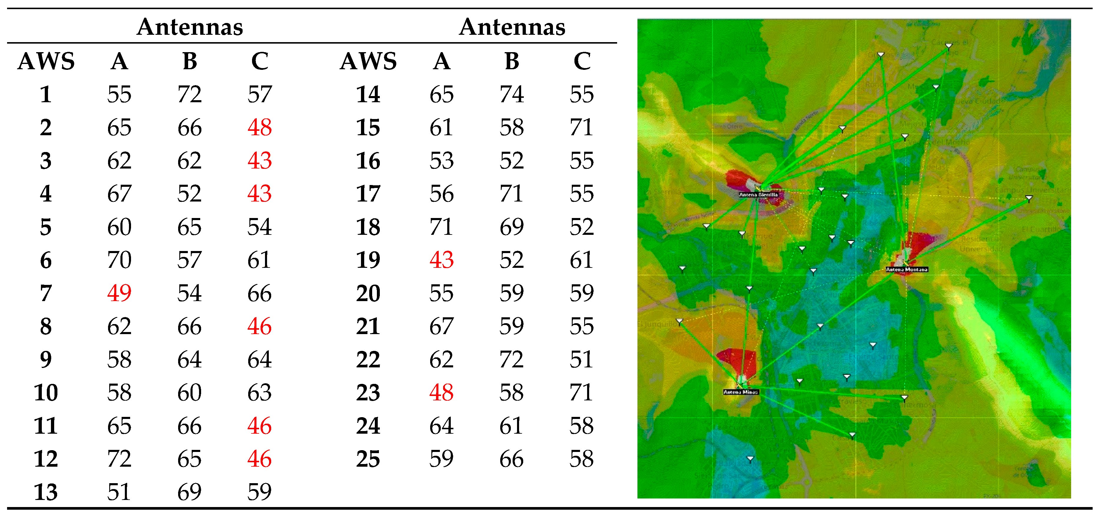
Figure 7.
Distribution and probability density of the records of each of the AWSs of Bs, Nt, WU and AEMET in different temperature ranges between August 1 and 26, 2024.
Figure 7.
Distribution and probability density of the records of each of the AWSs of Bs, Nt, WU and AEMET in different temperature ranges between August 1 and 26, 2024.
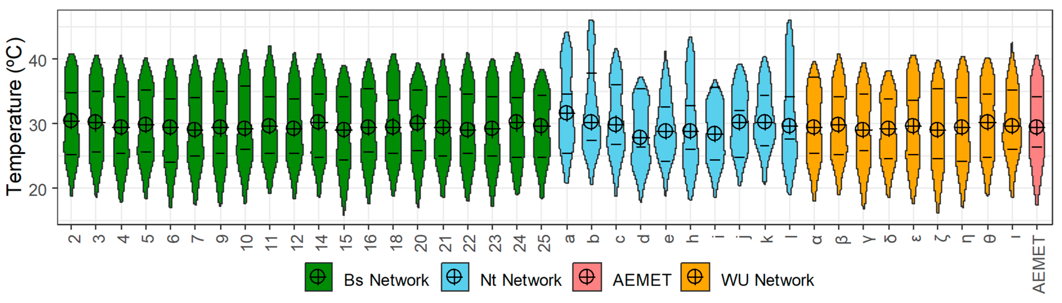
Figure 8.
Hourly oscillation of Bs, Nt, and WU, difference between the maximum and minimum values recorded at that hour by their AWSs, from August 1 to 26, 2024.
Figure 8.
Hourly oscillation of Bs, Nt, and WU, difference between the maximum and minimum values recorded at that hour by their AWSs, from August 1 to 26, 2024.
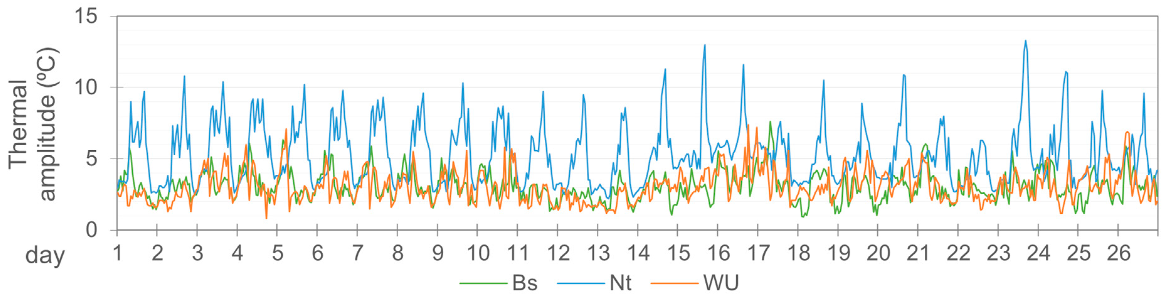
Figure 9.
Scatter plot and linear fit of the Control Points, from August 1 to 26, 2024.
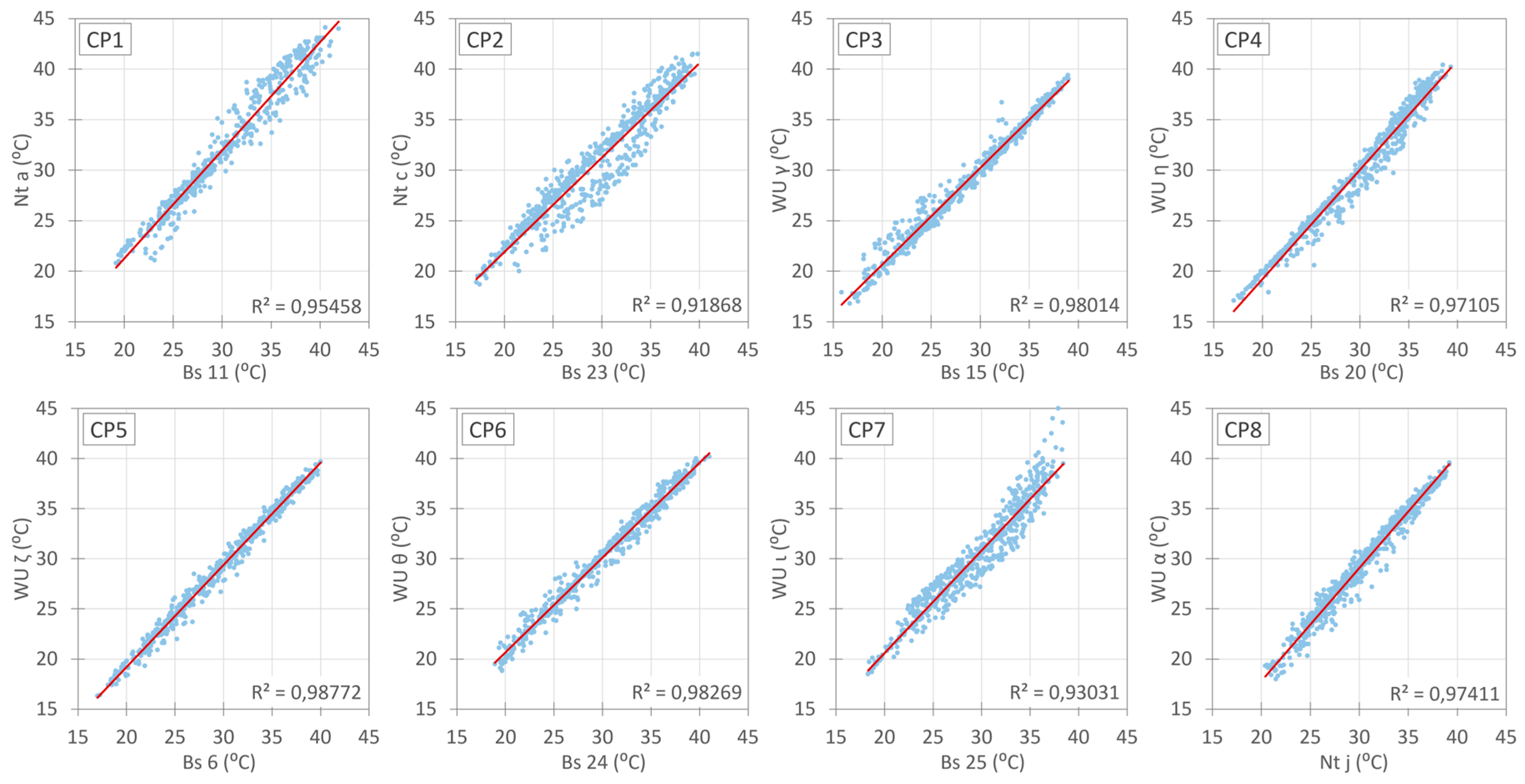
Figure 10.
Scatter plot of CP1 comparing Bs, Nt and WU AWSs, from August 1 to 26, 2024.
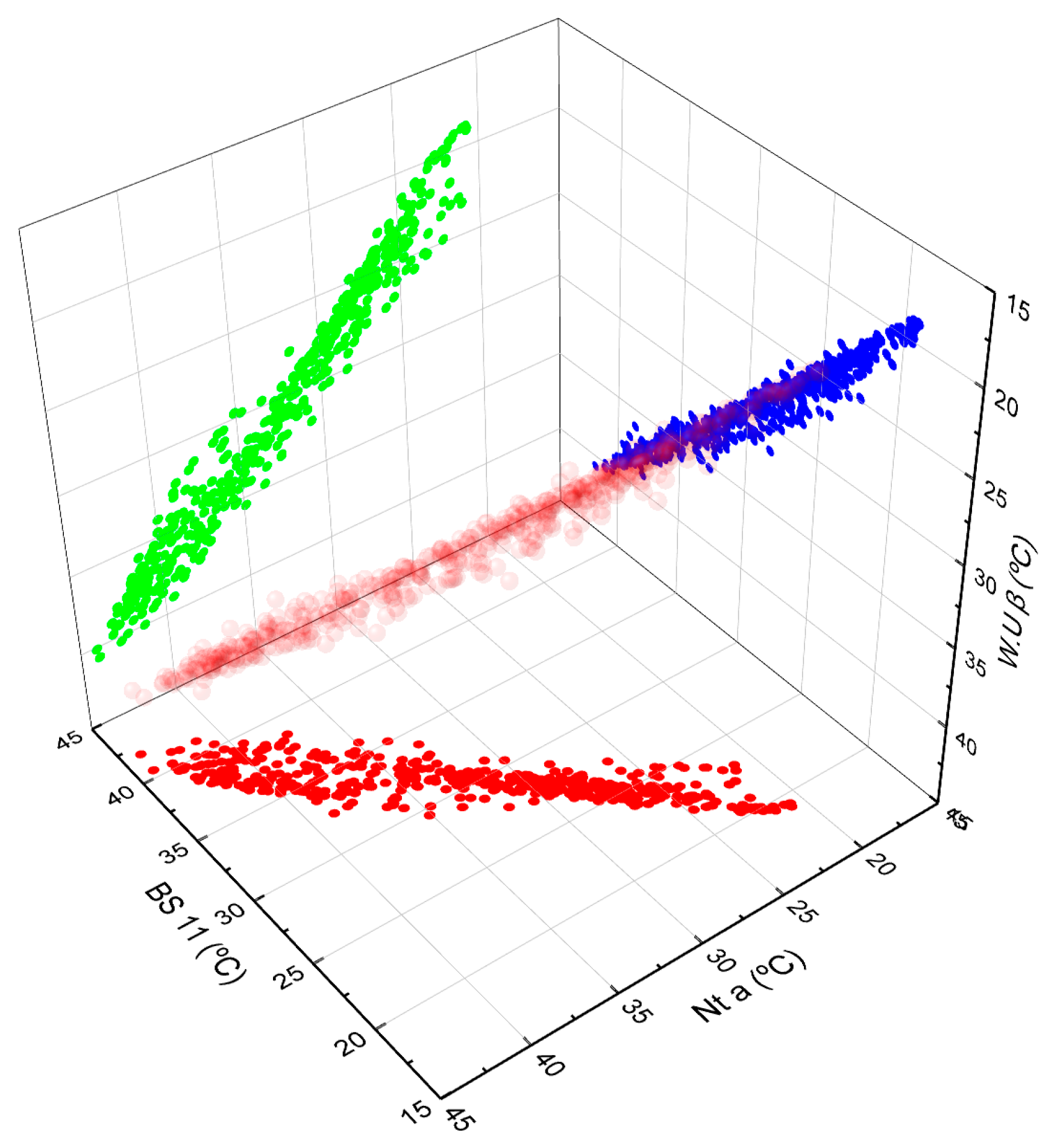
Figure 11.
Hourly evolution of AWSs temperatures at each of the monitoring points in the different networks during the week of August 12 to 18, 2024.
Figure 11.
Hourly evolution of AWSs temperatures at each of the monitoring points in the different networks during the week of August 12 to 18, 2024.
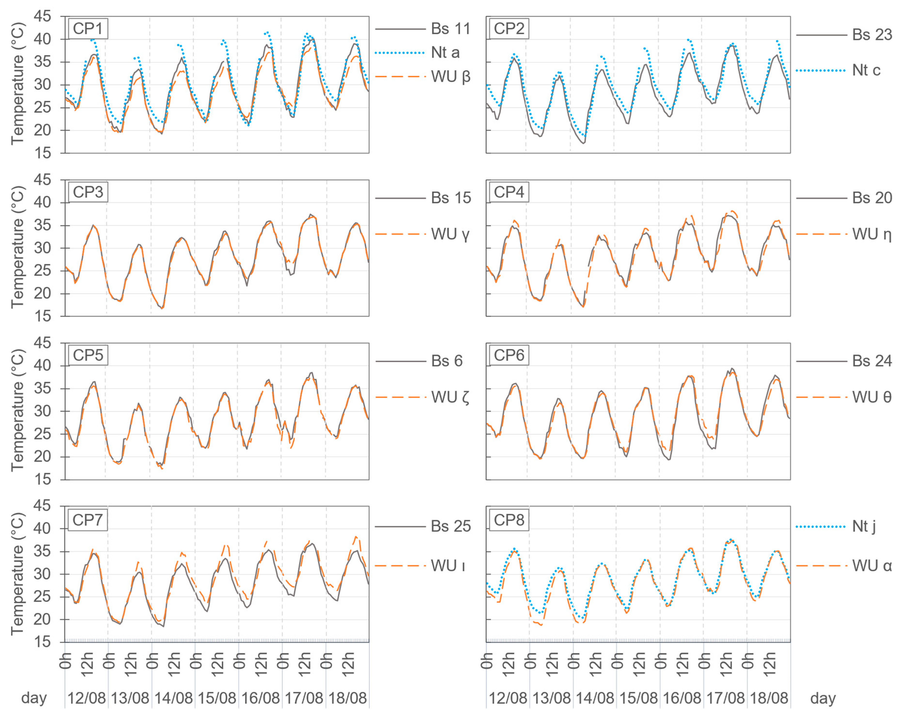
Figure 12.
Hourly evolution of AWSs temperatures for each zone (North, West, and South) for the week of August 12 to 18, 2024.
Figure 12.
Hourly evolution of AWSs temperatures for each zone (North, West, and South) for the week of August 12 to 18, 2024.
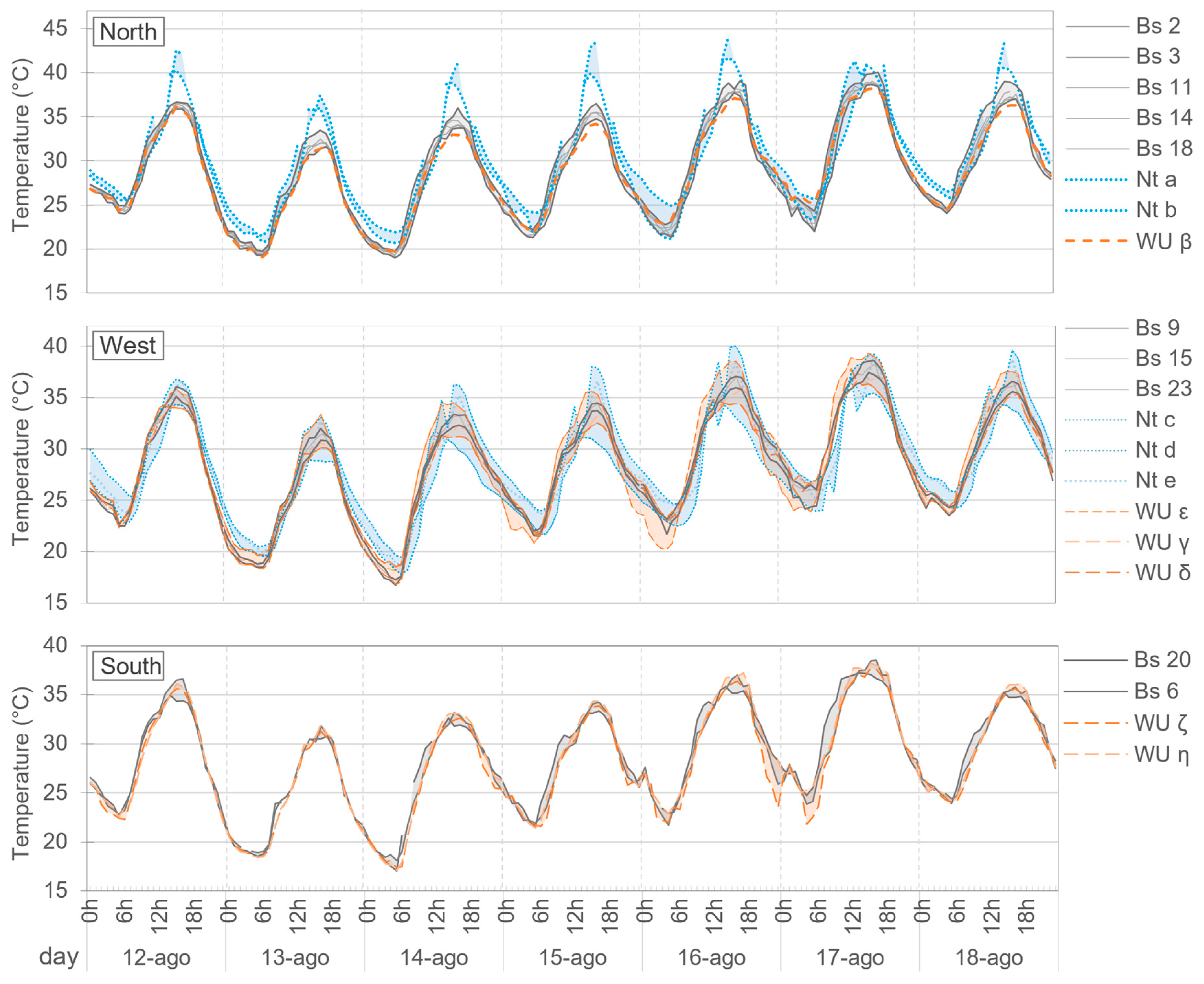
Table 1.
Temperature indicators in the week of August 12 to 18, 2024 in the different AWSs of the control points.
Table 1.
Temperature indicators in the week of August 12 to 18, 2024 in the different AWSs of the control points.
| Control point and AWS | Weekly amplitude (°C) | Minimum (°C) | Maximum (°C) | Weekly average (°C) | CDD (°C·day) | |||||
|---|---|---|---|---|---|---|---|---|---|---|
| Absolute | Daily average |
Absolute | Daily average |
Totals | Daytime (% of total) |
Nighttime (% of total) | ||||
| CP1 | Bs 11 | 20.8 | 19.3 | 21.8 | 40.1 | 37.1 | 29.4 | 141 | 94 (67%) | 46 (33%) |
| Nt a | 20.6 | 21.1 | 23.1 | 41.7 | 39.8 | 30.7 | 169 | 114 (68%) | 55 (32%) | |
| WU β | 19.1 | 19.1 | 22.3 | 38.2 | 35.2 | 28.6 | 141 | 94 (67%) | 47 (33%) | |
| CP2 | Bs 23 | 21.5 | 17.1 | 21.7 | 38.6 | 35.4 | 28.3 | 136 | 93 (69%) | 43 (31%) |
| Nt c | 21.4 | 18.7 | 23.6 | 40.1 | 37.6 | 29.9 | 159 | 101(64%) | 57 (36%) | |
| CP3 | Bs 15 | 20.8 | 16.7 | 21.2 | 37.5 | 34.4 | 28.0 | 133 | 90 (68%) | 43 (32%) |
| WU γ | 20.1 | 16.8 | 21.7 | 36.9 | 34.2 | 28.0 | 138 | 100 (72%) | 38 (28%) | |
| CP4 | Bs 20 | 20.1 | 17.1 | 21.6 | 37.2 | 34.3 | 28.5 | 138 | 95 (68%) | 44 (32%) |
| WU η | 21.1 | 17.1 | 21.6 | 38.2 | 35.3 | 28.4 | 136 | 94 (69%) | 42 (31%) | |
| CP5 | Bs 6 | 20.4 | 18.1 | 21.7 | 38.5 | 35.3 | 28.5 | 136 | 94 (69%) | 43 (31%) |
| WU ζ | 20.3 | 17.4 | 21.1 | 37.7 | 34.7 | 27.9 | 130 | 90 (70%) | 39 (30%) | |
| CP6 | Bs 24 | 20.1 | 19.4 | 21.2 | 39.4 | 36.3 | 28.7 | 140 | 100 (72%) | 40 (28%) |
| WU θ | 18.9 | 19.6 | 21.9 | 38.5 | 35.8 | 28.9 | 143 | 98 (69%) | 45 (31%) | |
| CP7 | Bs 25 | 18.3 | 18.4 | 22.1 | 36.7 | 34.0 | 28.1 | 135 | 90 (67%) | 45 (33%) |
| WU ι | 18.9 | 19.4 | 23.4 | 38.3 | 36.2 | 28.9 | 148 | 93 (63%) | 55 (37%) | |
| CP8 | Nt j | 17.2 | 20.4 | 23.3 | 37.6 | 34.4 | 29.0 | 146 | 94 (65%) | 52 (35%) |
| WU α | 18.6 | 18.8 | 22.1 | 37.4 | 34.2 | 28.2 | 135 | 90 (67%) | 45 (33%) | |
Table 2.
Temperature indicators for the week of August 12 to 18, 2024, in the different networks in the control zones.
Table 2.
Temperature indicators for the week of August 12 to 18, 2024, in the different networks in the control zones.
| No. of AWSs per network | Between AWSs of each network: absolute difference (°C) | Between networks | |||||||||
|---|---|---|---|---|---|---|---|---|---|---|---|
| Weekly amplitude (°C) | Average daily values (°C) |
Weekly average (°C) | CDD (°C·day) | ||||||||
| Totals | Daytime (% of total) |
Nighttime (% of total) |
|||||||||
| Max | Average | Min | Max | ||||||||
| North zone | |||||||||||
| Bs | 5 | 4.7 | 1.5 | 19.9 | 21.9 | 36.3 | 28.9 | 143 | 98 (69%) | 45 (31%) | |
| Nt | 2 | 6.2 | 2.0 | 22.8 | 23.5 | 41.2 | 30.7 | 168 | 112 (67%) | 56 (33%) | |
| WU* | 1 | - | - | 19.1 | 22.3 | 35.2 | 28.6 | 141 | 94 (67%) | 47 (33%) | |
| West zone | |||||||||||
| Bs | 3 | 2.1 | 0.8 | 21.1 | 21.6 | 35.0 | 28.3 | 135 | 92 (68%) | 43 (32%) | |
| Nt | 3 | 7.4 | 3.1 | 20.1 | 22.8 | 35.9 | 28.6 | 142 | 90 (63%) | 52 (37%) | |
| WU | 3 | 4.2 | 2.0 | 20.2 | 21.7 | 34.7 | 28.2 | 135 | 92 (68%) | 43 (32%) | |
| South zone | |||||||||||
| Bs | 2 | 4.2 | 0.8 | 20.3 | 21.6 | 34.8 | 28.5 | 137 | 94 (69%) | 43 (31%) | |
| Nt | 0 | ||||||||||
| WU | 2 | 4.8 | 0.7 | 20.7 | 23.5 | 35.0 | 28.1 | 133 | 92 (69%) | 41 (31%) | |
* As only one AWS is present in the network, differences between stations cannot be calculated. Reported maximum, minimum, range, mean values, and CCD correspond solely to this AWS.
Disclaimer/Publisher’s Note: The statements, opinions and data contained in all publications are solely those of the individual author(s) and contributor(s) and not of MDPI and/or the editor(s). MDPI and/or the editor(s) disclaim responsibility for any injury to people or property resulting from any ideas, methods, instructions or products referred to in the content. |
© 2025 by the authors. Licensee MDPI, Basel, Switzerland. This article is an open access article distributed under the terms and conditions of the Creative Commons Attribution (CC BY) license (http://creativecommons.org/licenses/by/4.0/).
Copyright: This open access article is published under a Creative Commons CC BY 4.0 license, which permit the free download, distribution, and reuse, provided that the author and preprint are cited in any reuse.


