
Submitted:
13 November 2024
Posted:
15 November 2024
You are already at the latest version
Abstract
The goal of this study is to describe a design architecture for a self-powered IoT (Internet of Things) sensor network that is currently being deployed at various locations throughout the Dallas-Fort Worth metroplex to measure and report on Particulate Matter (PM) concentrations. This system leverages diverse low-cost PM sensors, enhanced by machine learning for sensor calibration, with LoRaWAN connectivity for long-range data transmission. Sensors are GPS-enabled, allowing precise geospatial mapping of collected data, which can be integrated with urban air quality forecasting models and operational forecasting systems. To achieve energy self-sufficiency, the system uses a small-scale solar-powered solution, allowing it to operate independently from the grid, making it both cost-effective and suitable for remote locations. This novel approach leverages multiple operational modes based on power availability to optimize energy efficiency and prevent downtime. By dynamically adjusting system behavior according to power conditions, it ensures continuous operation while conserving energy during periods of reduced supply. This innovative strategy significantly enhances performance and resource management, improving system reliability and sustainability. This IoT network provides localized real-time air quality data, which has significant public health benefits, especially for vulnerable populations in densely populated urban environments. The project demonstrates the synergy between IoT sensor data, machine learning-enhanced calibration, and forecasting methods, contributing to scientific understanding of microenvironments, human exposure, and public health impacts of urban air quality. In addition, this study emphasizes open source design principles, promoting transparency, data quality, and reproducibility by exploring cost-effective sensor calibration techniques and adhering to open data standards. The next iteration of the sensors will include edge processing for short-term air quality forecasts.
Keywords:
LoRaWAN
; Particulate Matter
; Air Quality
; Wireless sensor networks
; IoT
; Smart City
1. Introduction
Aerosols are airborne particulates composed of both solid and liquid particles [1]. These aerosols, commonly known as Particulate Matter (PM), are linked to a multitude of issues pertaining to global climate effects and human health [2,3,4,5]. The concentration of Particulate Matter in the air is generally measured using two key parameters: PM2.5 and PM10. PM2.5 refers to the total mass of all airborne particles with a diameter of up to 2.5 microns, known as fine particulate matter, while PM10 encompasses all airborne particles with a diameter of up to 10 microns, known as coarse particulate matter.
The physiological effects of exposure to PM can be profound and varied, depending on the size and composition of the particles. Fine particulate matter (PM2.5) can penetrate deep into the lungs [6] and enter the bloodstream [7], causing short-term effects such as respiratory irritation [8], exacerbation of asthma [9], and acute cardiovascular events [10]. Long-term exposure to PM has been associated with chronic health issues, including chronic obstructive pulmonary disease (COPD) [11], lung cancer [12], and cardiovascular diseases [13], leading to significant morbidity and mortality [14,15]. Moreover, vulnerable populations—such as children, the elderly, and individuals with pre-existing health conditions—face heightened risks [16,17]. Children are particularly susceptible due to their developing respiratory systems, while the elderly often have compromised health that makes them more vulnerable to the deleterious effects of air pollution [18,19,20].
In addition to direct health impacts, PM exposure carries substantial socio-economic effects [21]. The economic burden associated with PM-related health issues can be significant, encompassing healthcare costs for treatment and management of chronic diseases, lost productivity due to illness, and diminished quality of life for affected individuals and families [22]. This burden disproportionately affects low-income communities [23], where access to healthcare may be limited. Economic disparities can hinder these populations’ ability to mitigate the impacts of PM exposure, making it essential to develop targeted public health interventions that address these inequalities.
Geographic disparities in PM exposure further complicate the health landscape. Urban areas, particularly those with high traffic and industrial activities, often experience higher concentrations of PM, resulting in worse health outcomes compared to rural areas [24,25]. Studies have shown that low-income neighborhoods in urban centers frequently encounter greater PM exposure due to environmental injustices, where socio-economic factors influence both the location of pollution sources and access to resources for health mitigation [26]. For instance, research has highlighted that communities situated near highways or industrial zones are more likely to suffer from higher rates of respiratory diseases and other health complications linked to PM exposure. By understanding these geographic disparities, it becomes evident that effective monitoring systems, such as Long Range Wide Area Network (LoRaWAN)-based sensors, are crucial for identifying pollution hot-spots and implementing targeted interventions to protect vulnerable populations.
Measurements that sufficiently capture the spatial and temporal variability of atmospheric components, like particulate matter, are essential for accurately characterizing these components at the neighborhood scale. In most cases, rather than the actual physical scales of variability, the available fiscal and computational resources determine the resolution of atmospheric observations and simulation. In medium and large cities, for example, only a small number of monitoring stations are typically present. The Dallas-Fort Worth metroplex, which has a population of seven million people, has only three regulatory grade airborne particulate sensors. The ease of sensor placement is influenced by a given location’s access to power and network resources.
The spatial scales are dependent on variables such as local weather, distribution of sources, and terrain, as evidenced by street level surveys conducted with data at less than a meter resolution [27]. The Smart City paradigm is synonymous with having an increased number of devices that can provide adequate coverage within a given geographic area [28,29].
As low-cost sensing systems gain traction, environmental monitoring initiatives are being expanded to engage the public more effectively. Traditional air quality monitoring systems typically utilize a wider array of sensors, eschew low-power networks, and tend to be more expensive. Low-power wireless technologies become increasingly valuable in scenarios where energy sources are unavailable or present challenges. Recently, research has shifted towards low-power wide area network (LPWAN) technologies, including Long Range Wide Area Network (LoRaWAN), Narrowband IoT (NB-IoT), LTE-M, and Sigfox [30,31,32,33]. Although all these technologies are energy-efficient, we have chosen LoRaWAN for its scalability [34], robustness [35], and cost-effectiveness [36]. In fact, LoRaWAN has been adopted for many IoT-related applications since its inception in 2013.
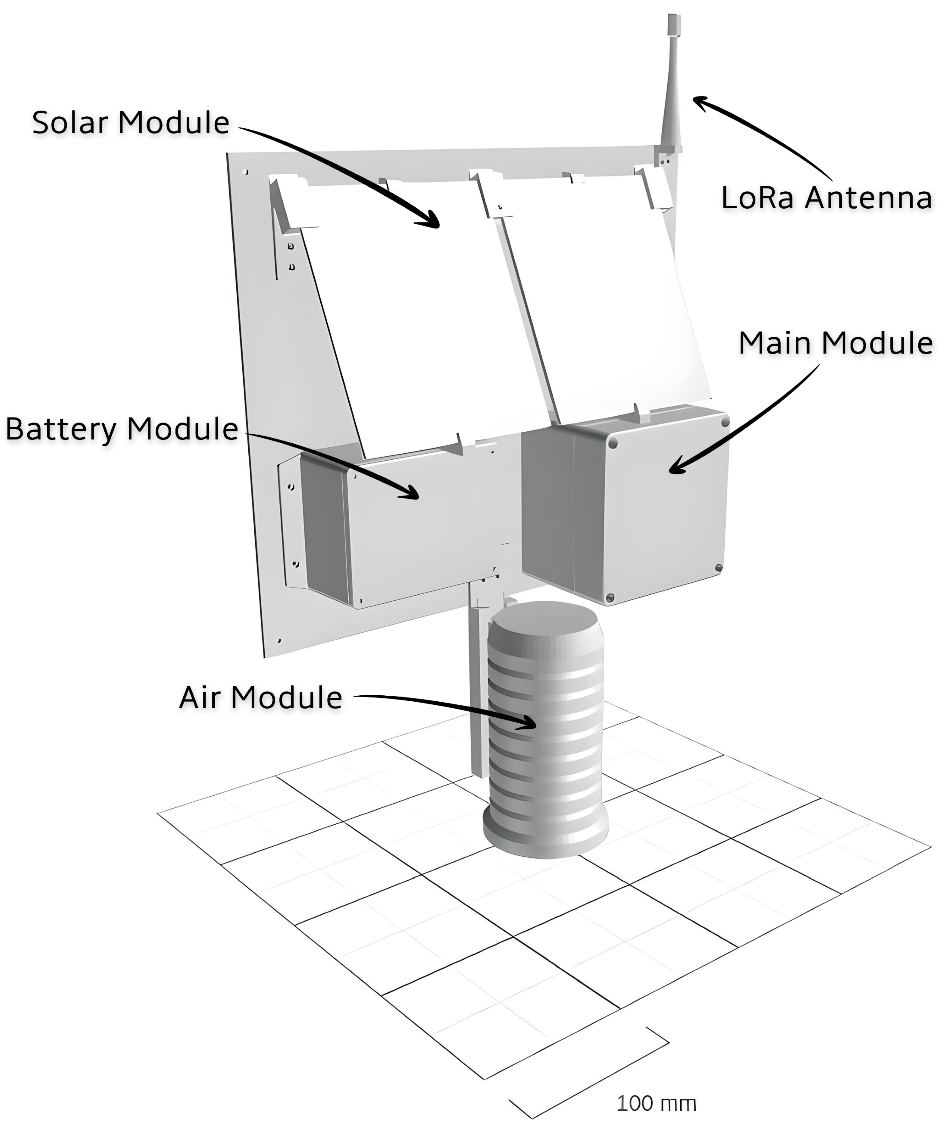
Figure 1.
External Physical Design: The physical build of the system consists of five separate modules, excluding the mounting back plate. Solar Module consists of a pair of 3 W solar panels while battery module consists of a 3.7 V, 6600 mAh Lithium Ion Battery Pack enclosed within a fireproof bag within a metal box. The main module contains the Power Control Unit (PCU), the Main Control Unit (MCU), as well as the low power, low current timer (TPL5110). The LoRa antenna is also mounted in the upper right corner of the mounting back plate.
2. Design
The following are the main elements included in the sensing configuration.
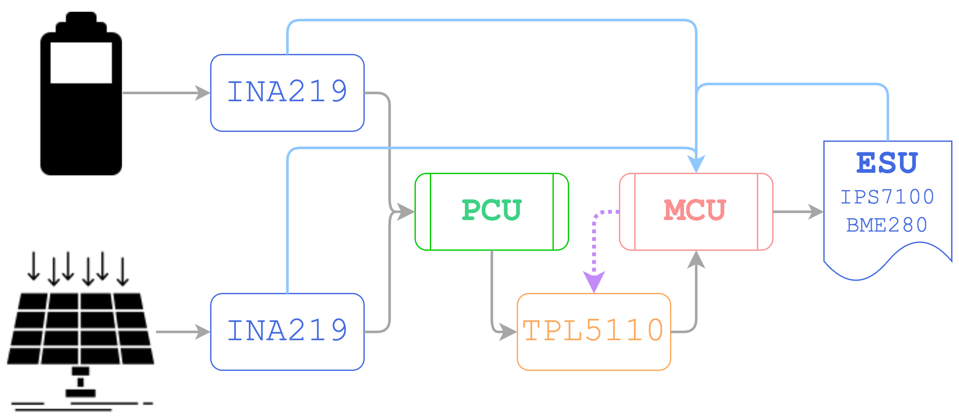
Figure 2.
System Design Architecture: LoRaWAN sensing units are comprised of a Main Control Unit (MCU), a Power Control Unit (PCU), an External Sensing Unit (ESU), two power sensors (INA219s), a low-power timer (TPL5110), a solar panel, and a battery. The figure illustrates the flow of power and data within the system. The gray arrows represent the power flow and the blue arrows represent the data flow. The dotted purple arrow represents the signal sent by the main control unit to put the system into sleep mode for the remainder of the current life cycle.
2.1. Main Controller Unit (MCU)
The MCU unit is where the main computing of the system is enacted. The MCU is comprised of three main components:
- ATSAMD21G18: 32-Bit ARM Cortex M0+
- RHF76-052DM: LoRaWAN Module
- L70: GPS Module
The combined unit is referred to as ‘Seeeduino LoRaWAN with GPS’ by the vendor and is considered to be an arduino development board that uses LoRaWAN protocol. ATMSAMD21G18 operates at 48 MHz and 3.3 V [37].
The incorporated LoRaWAN Module (RHF76-052DM) has dual band technology with 20 dBm max power being provided at 434 – 474 MHz and 14 dBm max power being provided at 868 – 915 MHz. LoRaWAN protocols Class A and Class C are supported by the module. All of these characteristics make it suitable for ultra-long range communications (up to 7 km in rural areas) and low power consumption [38]. The design presented in this paper uses the frequency band range of 902.3 – 914.9 MHz (USA LoRaWAN frequency spectrum) at 14 dBm and LoRaWAN protocol Class A for purposes of communication.
Additionally, the unit incorporates a low powered, small sized, GPS module. The L70 can communicate with a GPS receiver by NMEA 0183 (a combined electrical and data specification) [39]. This communication provides location information for the current application.
2.2. Power Control Unit (PCU)
The PCU is referred to as ‘Sunny Buddy - (Maximum Power Point Tracking) MPPT Solar Charger’ by the vendor and is comprised of the LT3652 circuit which is a complete monolithic step-down battery charger that operates over a 4.95 V to 32 V input voltage range. The PCU is connected both to the solar panel and to the battery, and it regulates the power to the MCU intelligently while keeping the battery charged throughout the day. A voltage regulation loop in the LT3652 reduces the charge current when the input voltage falls below a programmed level, which is determined by a resistor divider that we have set. If sufficient power is supplied by a solar panel, an input loop is used to maintain the LT3652’s maximum output. Charge current is terminated when the LT3652 falls below a tenth of the maximum charge current. Once charging is terminated, the LT3652 enters a low-current (85 A) standby mode. If the battery voltage falls 2.5% below the programmed float voltage, an auto-recharge feature initiates a new charging cycle [40].
2.3. INA219
The INA219 is an integrated I2C Bus and a shunt resistor. It monitors shunt current, shunt voltage (0 to 26 V), bus voltage and power by measuring the voltage drop across the shunt resistor. Operational voltage is 3 – 5.5 V. INA219 can be operated from -40 – 125 °C. I2C or SMBUS-compatible interface is used to communicate data with the MCU. Two separate INA219s are connected to the battery and the solar panel, and the flowing current from both sources is fed through to the PCU. For the I2C interface, two separate slave addresses are used to maintain uniqueness between the two INA219s.
2.4. TPL5110
Designed for battery operated or duty cycled applications, the TPL5110 Nano Timer is a low power, low current timer with an integrated MOSFET driver. Using only 35 nA of power, the TPL5110 is able to enable the power supply line so as to drastically reduce the overall system standby current during sleep time. As a result of its reduced power consumption, it can also be used with smaller batteries, which makes it well suited for energy harvesting and wireless sensor applications, such as the one being implemented. [41]. TPL5110 functions to shut down an MCU after a predetermined period of time and reactivate it after another predetermined period. This is particularly helpful if the system enters a sleep cycle when manual intervention is not possible in the field. However, the main purpose of the TPL5110 is to preserve energy efficiently. TPL5110 serves as a bridge between the PCU and MCU. In the design architecture of the system, embedded firmware is run inside of a MCU during its life cycle. TPL5110 allows us to choose the period in which the system will reset and rerun the firmware. A potentiometer is used to alter the period. In the current configuration, we used an external resistor to achieve this. The external resistor is configured so that a life cycle would last a maximum of 15 minutes, but in most instances the timer should shut off the power fed to the MCU much earlier depending on the amount of power stored by the battery and solar panel. This is accomplished through a signal sent through to the TPL5110 from the MCU after the power metrics are measured via the INA219s.
2.5. External Sensing Unit (ESU)
ESU consists of a Solar Radiation Shield that protects the sensing ensemble from climatic factors while maintaining accurate readings by maintaining airflow through the sensing elements. Two sensors are included in the system, the IPS7100 for particulate matter measurements and the BME280 for climate measurements.
-
IPS7100:This sensor is an Optical Particle Counter (OPC). It is also referred to as an Intelligent Particle Sensor (IPS). It detects particles with a diameter between 0.1 and 10 . At a rate of two cycles per second, the sensor can provide particle counts within 7 different bins within the specified range. IPS7100 also provides conventional particle mass fractions that are used to quantify air pollution, which include PM1, PM2.5, and PM10. Additionally, the IPS7100 provides measurements of PM0.1, PM0.3, PM0.5, and PM5. The IPS7100 can be used with both UART and I2C hardware communication protocols. In the present application, the hardware communication protocol I2C is used. With a low power consumption of 0.325 W during measurements and only 0.001365 W in sleep mode, this device is well-suited for solar and battery applications, such as the one described here [42].
-
BME280:Optical particle counters usually consider temperature, pressure, and humidity as bias factors. We added the Bosch BME280 sensor to account for such biases as well as report climate data. It is designed specifically for mobile and wearable applications. Compact and power-efficient, it provides us with crucial climate data. BME280 is a digital humidity, pressure, and temperature sensor that supports both SPI and I2C interfaces. It operates within a voltage range of 1.71 – 3.6 V [43]. In our configuration the device is set to run at 3.3 V using the I2C interface.
3. Operation
The sensing system is intended to obtain sensor measurements and transmit the data in a sustainable manner. The duration of a single firmware life cycle is 15 minutes. During a single life cycle, the first step is to read current battery and solar power voltages using the two INA219s and select a power mode. Figure 4 illustrates the different power modes. In the event that the sensor does not receive sufficient power, power mode 0 is set and the TPL5110 is used to set the system to sleep for the remaining duration of the current life-cycle.
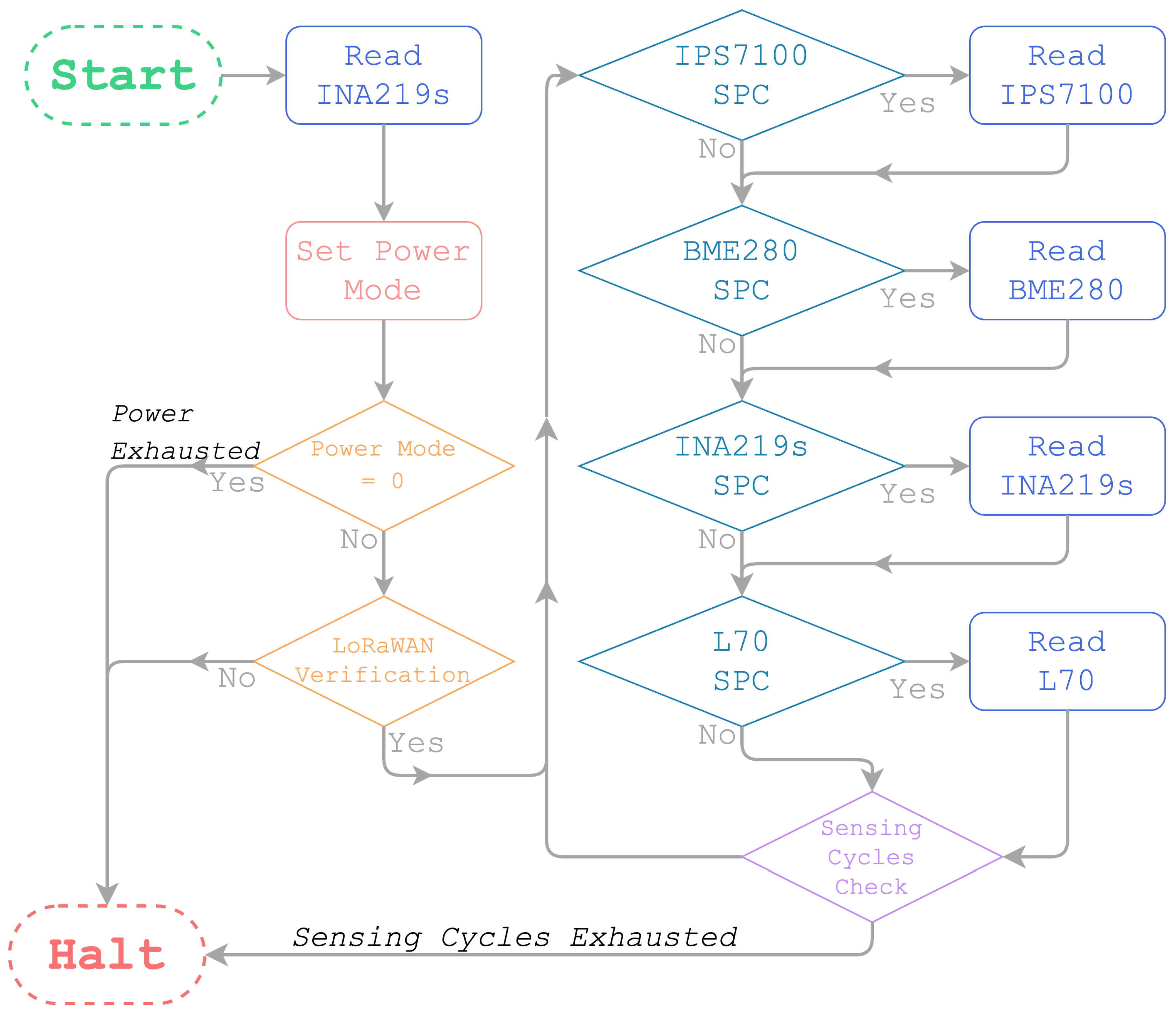
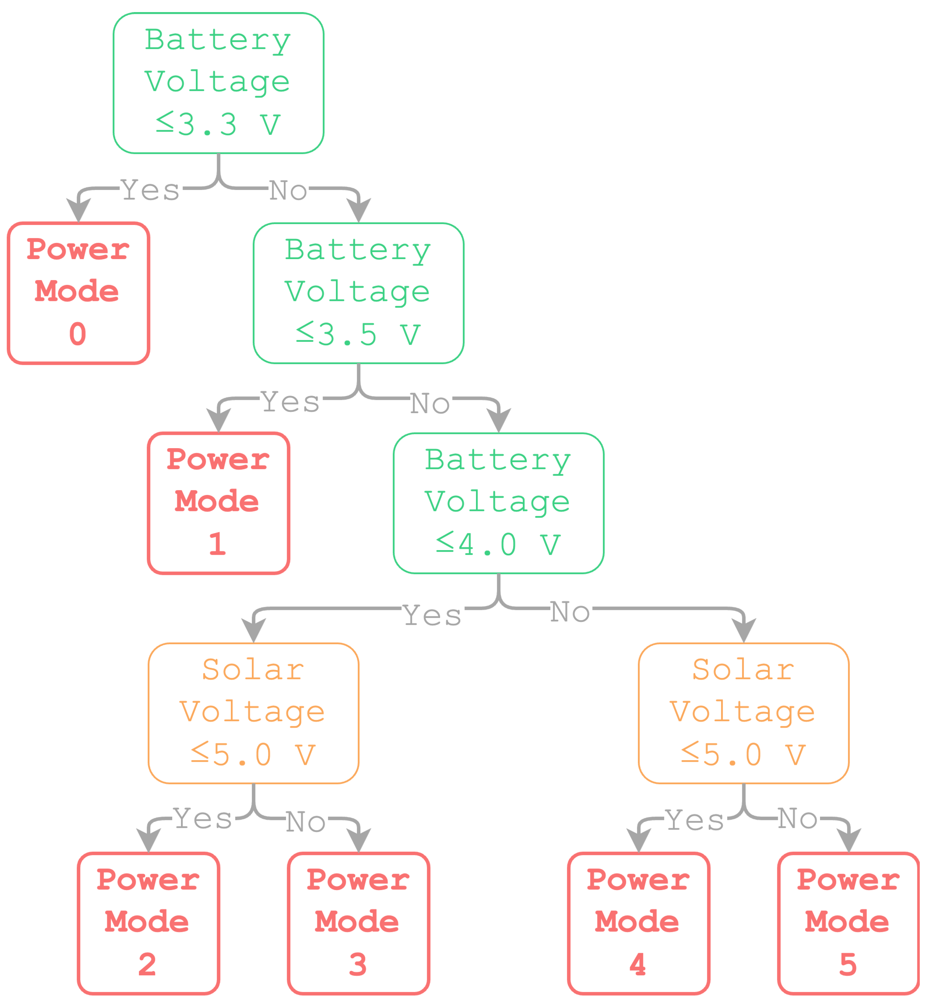
Figure 3.
Operation: The system is designed with power management in mind and initially makes power readings to select a predefined power mode. Depending on the power mode, the system will either halt or manage sensing operations and measurement frequency. The overall process is illustrated in this figure, where SPC denotes the "Sensing Period Check".
Figure 4.
Power Modes: In the beginning of each life cycle, the MCU determines a power mode for the system to be in, and the mode is solely determined by the output voltage from the solar panels and the current battery voltage. An illustration of how each power mode is set is presented in this figure.
In the event that the sensor has sufficient power, a LoRaWAN connection is established between the sensor node and the central gateway. Such a life cycle involves setting one of the following power modes: 1, 2, 3, 4 or 5. In order to ensure maximum security, each node has a unique ID and an application key that is specific to that ID. If the specifics match, the connection is made. By default, the data rate is set to 2 (3125 bits per second). In some cases, the network may adjust the data rate automatically in response to transmission characteristics. Once a successful connection has been established, Power Mode information is transmitted as the initial transmission of the current life cycle. Sensors are then initialized and the system is set in motion to collect data. For a given life cycle, the power modes also govern the number of sampling cycles and frequency of sampling for each sensor - for instance, the primary sensor (IPS7100) will vary its sampling frequency between 1 and 2 minutes based on the power mode selected for a given life cycle.
After the 15 minutes of the current life cycle is exhausted, the TPL5110 resets the system so that it initiates a new life cycle for the system.

Table 1.
Sensing Cycles for each Sensor
| Power Mode | Sensing Cycles | Sensing Period (minutes) | |||
|---|---|---|---|---|---|
| IPS7100 | BME280 | INA219s | L70 | ||
| 0 | 0 | - | - | - | - |
| 1 | 1 | - | - | - | - |
| 2 | 1 | - | - | - | - |
| 3 | 2 | 2 | 2 | 4 | 4 |
| 4 | 2 | 2 | 2 | 4 | 4 |
| 5 | ∞ | 1 | 1 | 3 | 3 |
For each life cycle of the sensing system, each sensor makes a predetermined number of measurements based on the power mode. When more than one measurement is made for a given sensor, the interval between each measurement is also controlled. This table reflects the number of sensing cycles along with the sensing periods.
4. Power Management
Careful steps have been taken to have sufficient power to run the system through out its field deployment. This is predominantly controlled via the power mode. Figure 4 gives the means in which power modes are set for each life cycle. In power mode 5, which is when the battery is fully charged as well as sufficient amount of sunlight is present, the firmware runs continuously without halting the system. On all the other power modes, after a predefined number of sensing cycles, the sensing system is halted to preserve continuous measurement of data throughout a given day, in all weather conditions. For example on power mode 1 and 2 the system will shut itself down after 1 sensing cycle which would only take around 7 minutes. And hence the system will sleep after for 8 (15 - 7) minutes of its ‘single life cycle’. And likewise on power mode 3, and 4 the system will shut itself down after 2 sensing cycles which would only take around 10 minutes. Although, power modes 1 and 2 as well as 3 and 4 are operationally similar for the current application, they are given specific power modes to cater future developments of the system, which is intended to have more sensing units.
5. Communication
This system is considered to be an end node within the LoRaWAN network. A central communication gateway, a component of a more comprehensive sensing suite referred to as a ‘Central Node’, receives the data collected by the system. Integrated into the ‘Central Node’ is a Dragino LIG16 with an SX1302 LoRa concentrator. As part of this system, the nodes and the gateway are connected by means of a LoRaWAN network operating at Sub-Band 8 (913.5 – 914.9 MHz) for up links.
In this architecture, the gateway is placed at the center, while the end nodes are arranged around it following a star topology. To activate end devices, this network uses Over-the-Air (OTAA) activation, since this is the most secure and reliable method. The system data is transmitted via packets with packet size and contents set by the sensor type. Details regarding the specific data packets are provided in Table 2. LoRaWAN gateways gather data packets and send them up to a LoRaWAN cloud where they are sorted out and distributed using an MQTT pipeline. The MQTT pipeline is used to cater both the SharedAirDFW public portal and an extensive analytical toolbox. Figure 5 provides a comprehensive overview of the complete network architecture.
6. Analytical Toolbox
To date, our sensor network has collected roughly 6 TB of data, and we expect our storage needs to continue to grow as we deploy new sensors each month. Additionally, the high degree of spatial variability necessitates a computational infrastructure that can manage thousands of individual time-series while providing real time analysis, pollution alerts, and eventually particle tracking and forecasting capabilities. To that end, we have developed a containerized solution comprising three open-source docker images: NodeRed, InfluxDB, and Grafana [44,45,46]. NodeRed allows us to easily ingest and process incoming sensor data in a simple graphical pipeline. This data is then injected by NodeRed into InfluxDB, a time-series database optimized for handling high frequency data from thousands of sources. Finally, Grafana is then connected to the database to enable dynamic, highly configurable, real-time visualization dashboards. These dashboards provide an interactable web interface to the data beyond what the current website enables.
6.1. NodeRed
Node-RED is a graphical programming tool that provides a collection of interfaces to hardware, data APIs, and more. Using a selection of processing nodes, the user generates a flow diagram representing the data ingestion and processing pipeline, which can be easily deployed with one click. A key advantage worth highlighting is that Node-RED’s low/no-code approach allows for an easily maintainable and scalable solution that can be adapted to new sensors and architectures. In Figure 6, the menu of nodes is visible on the left, while the deployment flow is shown in the center.
As discussed in the previous section, sensor data is published to a collection of MQTT topics in JSON format. The first step of the processing pipeline is to define a set of MQTT listeners that identify packets unique to each sensor type. When a message is identified, the packet is then processed into a JSON dictionary and subsequently parsed using a JavaScript node that allows for custom processing code. In this step, the relevant entries are parsed from the JSON dictionary and organized to be injected into the database. The full pipeline is illustrated on Figure 6.
Credentials for connecting to the MQTT broker as well as database access tokens are automatically loaded from user-supplied configuration files. The entirety of the flows themselves are saved as JSON files, enabling easy version-control via git. Once a pipeline is developed in the web interface, the relevant files are stored and loaded automatically by a docker upon deployment.
6.2. InfluxDB
InfluxDB was chosen as the sensor network database for its ease of use, time-series optimizations, and open-source status. In particular, a machine with a 4 core CPU and 4 GB of RAM can support up to 5,000 writes per second. Like NodeRed, InfluxDB has a web interface to enable data exploration and query generation. During the build process, our docker implementation generates a default bucket for the time series as well as default tokens to enable writing by NodeRed and reading by Grafana. A sample of the Data Explorer web interface is shown in Figure 7.
Complicated queries can be constructed using InfluxDB’s Flux query language, as it applies mathematical functions to compute statistical values and parameters. Queried data can be downloaded directly into CSV files for further analysis, or users can connect directly to the database by access token in their programming language of choice. Official client libraries exist for most popular languages, including Python, C++, and JavaScript.
6.3. Grafana
The final piece of the analysis toolbox is Grafana. When connected to InfluxDB, this tool enables the creation of a suite of real-time dashboards that visualize sensor data with a wide selection of graph types.
The dashboard is shown in Figure 8, in which a variety of visualizations have been selected to show real-time data for 7 consecutive days. Users can select a desired time range to query, or the dashboard can be set to automatically update at set rate (in the case of Figure 8, every 5 seconds). The size and location of each panel can be arranged by the user to suit their individual liking, and each panel can also expand for a full-screen view. Currently, dashboards exist for both Central and LoRa nodes. Dashboards depicting data from multiple nodes are also available.
These three tools combine together to form a comprehensive analysis and visualization platform. Future work will incorporate automatic alerts for pollution exceedances as well as additional external data sources providing users with unparalleled access to local air quality data.
7. Deployment
Each LoRaWAN device is developed to be put in real-life field environments. For the planned deployment, 10 LoRAWAN End Nodes are to be deployed with one Central Gateway. The system was designed and built for deployment throughout the Dallas Fortworth metroplex, and we plan on deploying 10 such systems, that would amount to 100 Nodes to be deployed. The system was in public use at the City of Joppa, TX under the Shared Air DFW initiative. Figure 9 showcases the first two sensors that were made available for public use in Joppa, TX.
8. Sensor Calibration
In this study, we focus on the use of low-cost air quality sensing systems. Governmental agencies primarily rely on Federal Reference Method (FRM) or Federal Equivalent Method (FEM) instruments to enforce air quality regulations due to their high accuracy. However, these systems typically cost between $25,000 and $100,000 USD, making widespread deployment financially challenging [47]. Additionally, FRM and FEM instruments often have lower sampling rates. This proposal introduces a low-cost sensing solution calibrated using co-located data collection with an FEM system employing an identical sensing package. This approach aims to provide a cost-effective alternative for air quality monitoring while maintaining data reliability and frequency.
A significant challenge for low-cost particulate matter (PM) sensors is the lack of integrated heaters to prevent hygroscopic growth, which often leads to the overestimation of particle sizes and consequently, PM mass concentrations. This issue is particularly pronounced when ambient temperature and dew point are closely aligned. Thus, the initial phase of our calibration process involves applying a humidity correction to the particle counts, followed by adjustments to the PM concentrations to ensure accurate measurement under varying humidity conditions. The humidity correction is based on the works of Di Antonio et al. and Dewage . The entire process of the sensor calibration is illustrated on Figure 10.
Previous research indicates that low-cost particulate matter (PM) sensors are affected by a range of environmental factors, such as humidity, temperature, and atmospheric pressure [50,51,52]. To improve the accuracy of these sensors, advanced machine learning algorithms are employed to calibrate humidity-adjusted readings, resulting in a more accurate representation of actual PM concentrations. This calibration process involved the co-location of similar sensing packages with LoRaWAN nodes near the Hawks Athletic Center in Fort Worth, Texas. Here, a Federal Equivalent Method (FEM) device, specifically the BAM 1022 - Beta Attenuation Mass Monitor, continuously gathered particulate data for comparison. The machine learning pipeline is deployed on the University of Texas at Dallas (UTD) cloud-based infrastructure via an MQTT pipeline endpoint. The corrected data is subsequently fed back into the analytical toolbox as an additional data point. The machine learning model is continuously updated. The initial dataset, collected from December 2023 to July 2024, will be expanded as new data becomes available, enabling ongoing refinement of the model.
Multiple approaches for non-linear, non-parametric machine learning were tested, including neural networks, support vector regression, and ensembles of decision trees. The best performance was achieved using an ensemble of decision trees with hyper-parameter optimization. The specific implementation used was RandomForestRegressor from Python’s scikit-learn library, which is based on the bagging method. Hyper-parameter optimization was performed to select the optimal values for the following attributes: number of estimators (trees), maximum depth of each tree, minimum samples required to split a node, minimum samples required at a leaf node, and the number of features to consider at each split. The optimal configuration was determined using a randomized search over these parameters to maximize model performance. A multivariate, non-linear, and non-parametric machine learning regression model was developed using eleven input variables. These variables included particle counts for seven particle sizes—0.1 , 0.3 , 0.5 , 1 , 2.5 , 5 , and 10 —each adjusted for humidity effects. In addition, four key environmental factors were included: atmospheric pressure, temperature, dew point, and relative humidity, all measured with the BME280 sensor. Together, these inputs allowed the model to account for both particulate and environmental dynamics in predicting outcomes. Figure 10 presents the machine learning model’s performance, as assessed on independent validation sets. Alongside this, a quantile-quantile plot illustrates model accuracy, and an additional plot highlights the most influential variables identified during the calibration phase.
8.1. Results
Figure 11 illustrates the results of a multivariate, non-linear, non-parametric machine learning regression for PM2.5. The scatter plot (Figure 11a) shows the log–log relationship between the PM abundance measurements from the BAM 1022 reference instrument (x-axis) and the PM abundance predicted by the machine learning calibration of the low-cost instrument (y-axis). For the training dataset, the model achieved an R2 value of 0.97 and a root mean square error (RMSE) of 12.13. On the independent validation dataset, the model attained an R2 value of 0.82 and an RMSE of 12.13, indicating robust predictive performance and strong generalizability across both training and validation datasets.
Figure 11b displays quantile–quantile (Q-Q) plots that compare the probability distribution functions (PDFs) of the PM abundance data from the BAM reference instrument with those from the machine learning-calibrated low-cost instrument. A straight line in a Q-Q plot indicates that the two distributions are identical, as it compares the percentiles of one PDF against the percentiles of the other. In this case, the plot reveals a straight line across the 25th to 75th percentiles, demonstrating the successful calibration of the low-cost instrument.
Figure 11c illustrates the relative importance of the input variables used in the machine learning calibration of the low-cost optical particle counter (IPS7100). The importance metric quantifies the increase in error when a specific input variable is omitted. The bar plots are arranged in descending order of importance, with the top bar representing the most influential variable. This analysis highlights the expected significance of the particle count for 2.5-micron particles, along with environmental factors such as temperature, pressure, dew point, and humidity, all of which contribute to the accurate calibration of the low-cost instrument against the reference instrument (BAM 1022).
After developing the machine learning model, we applied it successfully to data collected from sensors across our network. Figure 12 shows a time series from a LoRaWAN sensor deployed at the University of Texas at Dallas in Richardson, Texas, for October 2024. The figure compares the raw PM2.5 measurements from the IPS7100, the humidity-corrected PM2.5, and the machine learning-corrected PM2.5 values.
9. Discussion
This study presents a self-powered IoT network leveraging LoRaWAN technology for air quality monitoring, addressing the critical need for scalable, cost-effective environmental sensing systems that offer open-source access to high-frequency data through public portals, alongside transparent software and firmware availability. Although the existing literature [53,54,55,56,57] provides insights into some components of these technologies, this work integrates all essential elements into a comprehensive framework.
Through LoRaWAN, we enable both scientists and the public to collect data and securely transmit it to high-performance computing infrastructures for advanced analysis. This ‘citizen science’ model has gained momentum with the availability of affordable, high-precision sensors that reliably measure pollutants such as particulate matter. Many of these LoRaWAN nodes are now deployed within community areas, making real-time air quality monitoring accessible to local residents.
While FEM/FRM sensor networks offer reliable but low-frequency monitoring, they are costly and can introduce latency. Our objective was to create a low-cost alternative that caters to resource-conscious settings, maintaining comparable data quality through machine learning to achieve higher frequency and minimal latency. Furthermore, our devices utilize LoRaWAN for data transmission, avoiding the need for complex and expensive networking solutions like Wi-Fi.
10. Challenges and Future Directions
One of the key challenges encountered during the deployment of these sensors was the limited communication range in urban environments, where access to mounting locations with a clear line of sight was constrained. Consequently, the communication range between the LoRaWAN node and the gateway was restricted to less than one mile. To overcome this limitation, ongoing research is exploring the use of high-powered LoRaWAN radios with a maximum output of 20 , in contrast to the 14 radios used in the initial deployment. In addition, consultations with industry experts have been conducted to identify optimal antenna configurations aimed at improving signal strength and range.
Looking ahead, efforts are underway to expand the proposed system by integrating larger batteries and more energy-efficient solar panels. Currently, the battery life spans from 6 to 12 months, limiting the deployment and data collection capacity. The planned upgrades will enable the integration of additional sensors, allowing for the collection of more comprehensive measurements and enhancing the overall quality of the data. Furthermore, we are advancing our machine learning training processes, which are being conducted in both controlled laboratory environmental chambers and a mobile laboratory mounted on an electric vehicle. This approach is intended to improve the accuracy and reliability of the model, complementing ongoing training efforts with the sensing system deployed in Fort Worth, TX.
Supplementary Materials
The firmware has been made publicly available. The firmware for the LoRaWAN end node is available in the Zenodo data store: https://doi.org/10.5281/zenodo.6727816 (accessed on 23 June 2022). The SharedAirDFW public portal, which provides up to date particulate matter data from the LoRaWAN end nodes, can be accessed at https://www.sharedairdfw.com/.
Author Contributions
Specify each author’s contribution to this work respectively.
Funding
We acknowledge funding from the following sources: Earth Day Texas; Downwinders at Risk; the City of Plano; TRECIS CC* Cyberteam (NSF #2019135); NSF OAC-2115094 Award; AFWERX AFX23D-TCSO1 Proposal # F2-17492; The US Army (Dense Urban Environment Dosimetry for Actionable Information and Recording Exposure, U.S. Army Medical Research Acquisition Activity, BAA CDMRP Grant Log #BA170483), EPA 16th Annual P3 Awards Grant Number 83996501, entitled Machine Learning-Calculated Low-Cost Sensing, The Texas National Security Network Excellence Fund Award for Environmental Sensing Security Sentinels, and the SOFWERX Award for Machine Learning for Robotic Team and NSF Award OAC-2115094.
Acknowledgments
The authors extend their sincere gratitude to Eric Lenington, Andy Slote and Chris Simonds from Object Spectrum, LLC, for their unwavering support in the realm of LoRaWAN technologies. We wish to express our deep appreciation to the esteemed Undergraduate Research Students - Aaron Barbosa, Berkley Shofner (Clark Research Program), John Charles Sadler, Julia Boah Kim, and Giakhanh Huu Hoang - for their exceptional contributions that have played a crucial role in shaping the trajectory of our ongoing research. A special acknowledgment is dedicated to the distinguished Undergraduate Senior Design Students - Kameron Noorbakhsh, Nicholas Steele, Nikhil Nair, Jake Schroder, Benjamin Hogan, Jacob Scheller, Jonah Duncan, Getenet Demsie, Nathan Nguyen, Bryanth Fung, Keigo Ma, Robert Wu, Kangzhi Zhao, Sidney Evans, Kevin Flores, Fawaz Khurram, Veronica Ramirez, Daniel Yustana, Keshav Dhamanwala, Aditya Agrawal, Tommy Symalla, Dien Tran, Michael Villordon, Basil El-Hindi, George Yi, Eric Zhang, Trent Haines, and Noah Barber. Your collective endeavors have significantly enhanced our public sensing portal, sharedairdfw.com. We also express our profound gratitude to the high school students who generously volunteered their time and expertise. Inbar Leibovich and Shrey Joshi - your unwavering enthusiasm and dedication have been integral to the success of our projects, and your invaluable contributions are acknowledged with deep appreciation.
Conflicts of Interest
The author has declared that no competing interests exist.
References
- McMurry, P.H. A review of atmospheric aerosol measurements. Atmospheric Environment 2000, 34, 1959–1999. [Google Scholar] [CrossRef]
- Yang, Y.; Ruan, Z.; Wang, X.; Yang, Y.; Mason, T.G.; Lin, H.; Tian, L. Short-term and long-term exposures to fine particulate matter constituents and health: a systematic review and meta-analysis. Environmental pollution 2019, 247, 874–882. [Google Scholar] [CrossRef] [PubMed]
- Hime, N.J.; Marks, G.B.; Cowie, C.T. A comparison of the health effects of ambient particulate matter air pollution from five emission sources. International journal of environmental research and public health 2018, 15, 1206. [Google Scholar] [CrossRef]
- Wu, W.; Jin, Y.; Carlsten, C. Inflammatory health effects of indoor and outdoor particulate matter. Journal of Allergy and Clinical Immunology 2018, 141, 833–844. [Google Scholar] [CrossRef] [PubMed]
- Ali, M.U.; Liu, G.; Yousaf, B.; Ullah, H.; Abbas, Q.; Munir, M.A.M. A systematic review on global pollution status of particulate matter-associated potential toxic elements and health perspectives in urban environment. Environmental geochemistry and health 2019, 41, 1131–1162. [Google Scholar] [CrossRef] [PubMed]
- Li, R.; Zhou, R.; Zhang, J. Function of PM2. 5 in the pathogenesis of lung cancer and chronic airway inflammatory diseases. Oncology letters 2018, 15, 7506–7514. [Google Scholar] [CrossRef]
- Thangavel, P.; Park, D.; Lee, Y.C. Recent insights into particulate matter (PM2. 5)-mediated toxicity in humans: an overview. International journal of environmental research and public health 2022, 19, 7511. [Google Scholar] [CrossRef]
- Xing, Y.F.; Xu, Y.H.; Shi, M.H.; Lian, Y.X. The impact of PM2. 5 on the human respiratory system. Journal of thoracic disease 2016, 8, E69. [Google Scholar] [CrossRef]
- Loftus, C.; Yost, M.; Sampson, P.; Arias, G.; Torres, E.; Vasquez, V.B.; Bhatti, P.; Karr, C. Regional PM2. 5 and asthma morbidity in an agricultural community: a panel study. Environmental research 2015, 136, 505–512. [Google Scholar] [CrossRef]
- Wang, C.; Tu, Y.; Yu, Z.; Lu, R. PM2. 5 and cardiovascular diseases in the elderly: an overview. International journal of environmental research and public health 2015, 12, 8187–8197. [Google Scholar] [CrossRef]
- Ni, L.; Chuang, C.C.; Zuo, L. Fine particulate matter in acute exacerbation of COPD. Frontiers in physiology 2015, 6, 294. [Google Scholar] [CrossRef] [PubMed]
- Hamra, G.B.; Guha, N.; Cohen, A.; Laden, F.; Raaschou-Nielsen, O.; Samet, J.M.; Vineis, P.; Forastiere, F.; Saldiva, P.; Yorifuji, T.; others. Outdoor particulate matter exposure and lung cancer: a systematic review and meta-analysis. Environmental health perspectives 2014. [CrossRef]
- Du, Y.; Xu, X.; Chu, M.; Guo, Y.; Wang, J. Air particulate matter and cardiovascular disease: the epidemiological, biomedical and clinical evidence. Journal of thoracic disease 2016, 8, E8. [Google Scholar] [CrossRef] [PubMed]
- Lippmann, M.; Ito, K.; Nadas, A.; Burnett, R.T. Association of particulate matter components with daily mortality and morbidity in urban populations. Research Report (Health Effects Institute) 2000, pp. 5–72.
- Fang, Y.; Naik, V.; Horowitz, L.; Mauzerall, D.L. Air pollution and associated human mortality: the role of air pollutant emissions, climate change and methane concentration increases from the preindustrial period to present. Atmospheric Chemistry and Physics 2013, 13, 1377–1394. [Google Scholar] [CrossRef]
- Grigg, J. Particulate matter exposure in children: relevance to chronic obstructive pulmonary disease. Proceedings of the American Thoracic Society 2009, 6, 564–569. [Google Scholar] [CrossRef]
- Ranft, U.; Schikowski, T.; Sugiri, D.; Krutmann, J.; Krämer, U. Long-term exposure to traffic-related particulate matter impairs cognitive function in the elderly. Environmental research 2009, 109, 1004–1011. [Google Scholar] [CrossRef]
- Dondi, A.; Carbone, C.; Manieri, E.; Zama, D.; Del Bono, C.; Betti, L.; Biagi, C.; Lanari, M. Outdoor air pollution and childhood respiratory disease: the role of oxidative stress. International journal of molecular sciences 2023, 24, 4345. [Google Scholar] [CrossRef]
- Aithal, S.S.; Sachdeva, I.; Kurmi, O.P. Air quality and respiratory health in children. Breathe 2023, 19. [Google Scholar] [CrossRef]
- Karimi, B.; Samadi, S. Long-term exposure to air pollution on cardio-respiratory, and lung cancer mortality: a systematic review and meta-analysis. Journal of Environmental Health Science and Engineering 2024, pp. 1–21. [CrossRef]
- Zhou, C.; Chen, J.; Wang, S. Examining the effects of socioeconomic development on fine particulate matter (PM2. 5) in China’s cities using spatial regression and the geographical detector technique. Science of the Total Environment 2018, 619, 436–445. [Google Scholar] [CrossRef]
- Zhang, M.; Song, Y.; Cai, X.; Zhou, J. Economic assessment of the health effects related to particulate matter pollution in 111 Chinese cities by using economic burden of disease analysis. Journal of environmental management 2008, 88, 947–954. [Google Scholar] [CrossRef]
- Bell, M.L.; Ebisu, K. Environmental inequality in exposures to airborne particulate matter components in the United States. Environmental health perspectives 2012, 120, 1699–1704. [Google Scholar] [CrossRef]
- Sun, Y. Environmental correlates of mortality: How does air pollution contribute to geographic disparities in cardiovascular disease mortality? Population and Environment 2024, 46, 1. [Google Scholar] [CrossRef]
- Colmer, J.; Hardman, I.; Shimshack, J.; Voorheis, J. Disparities in PM2. 5 air pollution in the United States. Science 2020, 369, 575–578. [Google Scholar] [CrossRef] [PubMed]
- Tessum, C.W.; Apte, J.S.; Goodkind, A.L.; Muller, N.Z.; Mullins, K.A.; Paolella, D.A.; Polasky, S.; Springer, N.P.; Thakrar, S.K.; Marshall, J.D.; others. Inequity in consumption of goods and services adds to racial–ethnic disparities in air pollution exposure. Proceedings of the National Academy of Sciences 2019, 116, 6001–6006. [Google Scholar] [CrossRef] [PubMed]
- Harrison, W.A.; Lary, D.; Nathan, B.; Moore, A.G.; others. The neighborhood scale variability of airborne particulates. Journal of Environmental Protection 2015, 6, 464. [Google Scholar] [CrossRef]
- Lanza, J.; Sánchez, L.; Muñoz, L.; Galache, J.A.; Sotres, P.; Santana, J.R.; Gutiérrez, V. Large-Scale Mobile Sensing Enabled Internet-of-Things Testbed for Smart City Services. International Journal of Distributed Sensor Networks 2015, 11, 785061. [Google Scholar] [CrossRef]
- Nam, T.; Pardo, T.A. Conceptualizing smart city with dimensions of technology, people, and institutions. Proceedings of the 12th annual international digital government research conference: digital government innovation in challenging times, 2011, pp. 282–291.
- Bonilla, V.; Campoverde, B.; Yoo, S.G. A Systematic Literature Review of LoRaWAN: Sensors and Applications. Sensors 2023, 23, 8440. [Google Scholar] [CrossRef]
- Chaudhari, B.S.; Zennaro, M.; Borkar, S. LPWAN technologies: Emerging application characteristics, requirements, and design considerations. Future Internet 2020, 12, 46. [Google Scholar] [CrossRef]
- Mekki, K.; Bajic, E.; Chaxel, F.; Meyer, F. A comparative study of LPWAN technologies for large-scale IoT deployment. ICT express 2019, 5, 1–7. [Google Scholar] [CrossRef]
- Iqbal, M.; Abdullah, A.Y.M.; Shabnam, F. An application based comparative study of LPWAN technologies for IoT environment. 2020 IEEE Region 10 Symposium (TENSYMP). IEEE, 2020, pp. 1857–1860.
- Van den Abeele, F.; Haxhibeqiri, J.; Moerman, I.; Hoebeke, J. Scalability analysis of large-scale LoRaWAN networks in ns-3. IEEE Internet of Things Journal 2017, 4, 2186–2198. [Google Scholar] [CrossRef]
- El Chall, R.; Lahoud, S.; El Helou, M. LoRaWAN network: Radio propagation models and performance evaluation in various environments in Lebanon. IEEE Internet of Things Journal 2019, 6, 2366–2378. [Google Scholar] [CrossRef]
- Yousuf, A.M.; Rochester, E.M.; Ghaderi, M. A low-cost LoRaWAN testbed for IoT: Implementation and measurements. 2018 IEEE 4th World Forum on Internet of Things (WF-IoT), 2018, pp. 361–366. [CrossRef]
- Microchip Technology Inc. SAM D21/DA1 Family, Low-Power, 32-bit Cortex-M0+ MCU with Advanced Analog and PWM, 2021. DS40001882G.
- RisingHF. RHF-DS01500, RHF76-052 LoRaWAN Module, 2015. Rev.03 2015-01-25.
- Quectel Wireless Solutions Co., Ltd. L70 GPS, Protocol Specification, 2015.
- Linear Technology Corporation. LT3652, Power Tracking 2A Battery Charger for Solar Power, 2010. LT 1215 REV E.
- Texas Instruments. TPL5110 Nano-power System Timer for Power Gating, 2015. SNAS650 –JANUARY 2015–REVISED JANUARY 2015.
- Piera Systems. 305 / 3100 / 525 / 5100 / 7100, Photon Counting Intelligent Particle Sensor for Accurate Air Quality Monitoring Product Specification, 2021. IPS Datasheet V1.1.8.
- Bosch Sensortec Gmbh. BME280, Combined humidity and pressure sensor, 2018. BST-BME280-DS002-15.
- NodeRed. https://nodered.org/about/. Accessed: 2022-6-28.
- InfluxDB. https://www.influxdata.com/products/influxdb/. Accessed: 2022-6-28.
- Grafana. https://grafana.com/grafana/. Accessed: 2022-6-28.
- Lowther, S.D.; Jones, K.C.; Wang, X.; Whyatt, J.D.; Wild, O.; Booker, D. Particulate matter measurement indoors: a review of metrics, sensors, needs, and applications. Environmental science & technology 2019, 53, 11644–11656. [Google Scholar]
- Di Antonio, A.; Popoola, O.A.; Ouyang, B.; Saffell, J.; Jones, R.L. Developing a relative humidity correction for low-cost sensors measuring ambient particulate matter. Sensors 2018, 18, 2790. [Google Scholar] [CrossRef]
- Dewage, P.M.H. PHYSICAL SENSING OF AIRBORNE PARTICULATES USING COMPLEMENTARY IN-SITU AND REMOTE SENSING APPROACHES. PhD thesis, 2024.
- Wijeratne, L.O.; Kiv, D.R.; Aker, A.R.; Talebi, S.; Lary, D.J. Using Machine Learning for the Calibration of Airborne Particulate Sensors. Sensors 2020, 20, 99. [Google Scholar] [CrossRef] [PubMed]
- Kliengchuay, W.; Cooper Meeyai, A.; Worakhunpiset, S.; Tantrakarnapa, K. Relationships between meteorological parameters and particulate matter in Mae Hong Son province, Thailand. International Journal of Environmental Research and Public Health 2018, 15, 2801. [Google Scholar] [CrossRef] [PubMed]
- Tian, G.; Qiao, Z.; Xu, X. Characteristics of particulate matter (PM10) and its relationship with meteorological factors during 2001–2012 in Beijing. Environmental pollution 2014, 192, 266–274. [Google Scholar] [CrossRef]
- Thu, M.Y.; Htun, W.; Aung, Y.L.; Shwe, P.E.E.; Tun, N.M. Smart air quality monitoring system with LoRaWAN. 2018 IEEE International Conference on Internet of Things and Intelligence System (IOTAIS). IEEE, 2018, pp. 10–15.
- Johnston, S.J.; Basford, P.J.; Bulot, F.M.; Apetroaie-Cristea, M.; Easton, N.H.; Davenport, C.; Foster, G.L.; Loxham, M.; Morris, A.K.; Cox, S.J. City scale particulate matter monitoring using LoRaWAN based air quality IoT devices. Sensors 2019, 19, 209. [Google Scholar] [CrossRef]
- Howerton, J.M.; Schenck, B.L. The deployment of a LoRaWAN-based IoT air quality sensor network for public good. 2020 Systems and Information Engineering Design Symposium (SIEDS). IEEE, 2020, pp. 1–6.
- Jabbar, W.A.; Subramaniam, T.; Ong, A.E.; Shu’Ib, M.I.; Wu, W.; De Oliveira, M.A. LoRaWAN-based IoT system implementation for long-range outdoor air quality monitoring. Internet of Things 2022, 19, 100540. [Google Scholar] [CrossRef]
- Candia, A.; Represa, S.N.; Giuliani, D.; Luengo, M.A.; Porta, A.A.; Marrone, L.A. Solutions for SmartCities: proposal of a monitoring system of air quality based on a LoRaWAN network with low-cost sensors. 2018 Congreso Argentino de Ciencias de la Informática y Desarrollos de Investigación (CACIDI). IEEE, 2018, pp. 1–6.
Figure 5.
Network Architecture: In addition to LoRaWAN end nodes (a), the network consists of a LoRaWAN gateway embedded within an integrated sensing suite called ‘The Central Node’ (b), a LoRaWAN cloud (c) utilising the open-source ChirpStack LoRaWAN Network Server, the Shared Air DFW public portal (d) that provides access to up-to-date Sensor Data, as well as a comprehensive analytical toolbox (e) using influxDB, Grafana, and Node-Red.
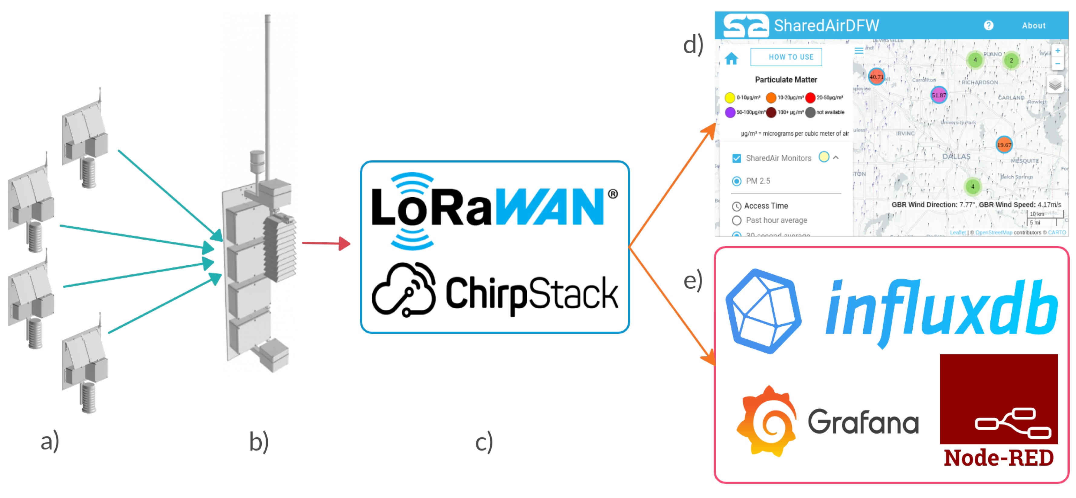
Figure 6.
NodeRed Interface: Node-RED web interface: A series of processing nodes are defined and connected sequentially from left to right, forming a processing flow. The flow starts with the collection of MQTT packets on the left, which are then converted into JSON dictionaries. These dictionaries are parsed and subsequently injected into InfluxDB.
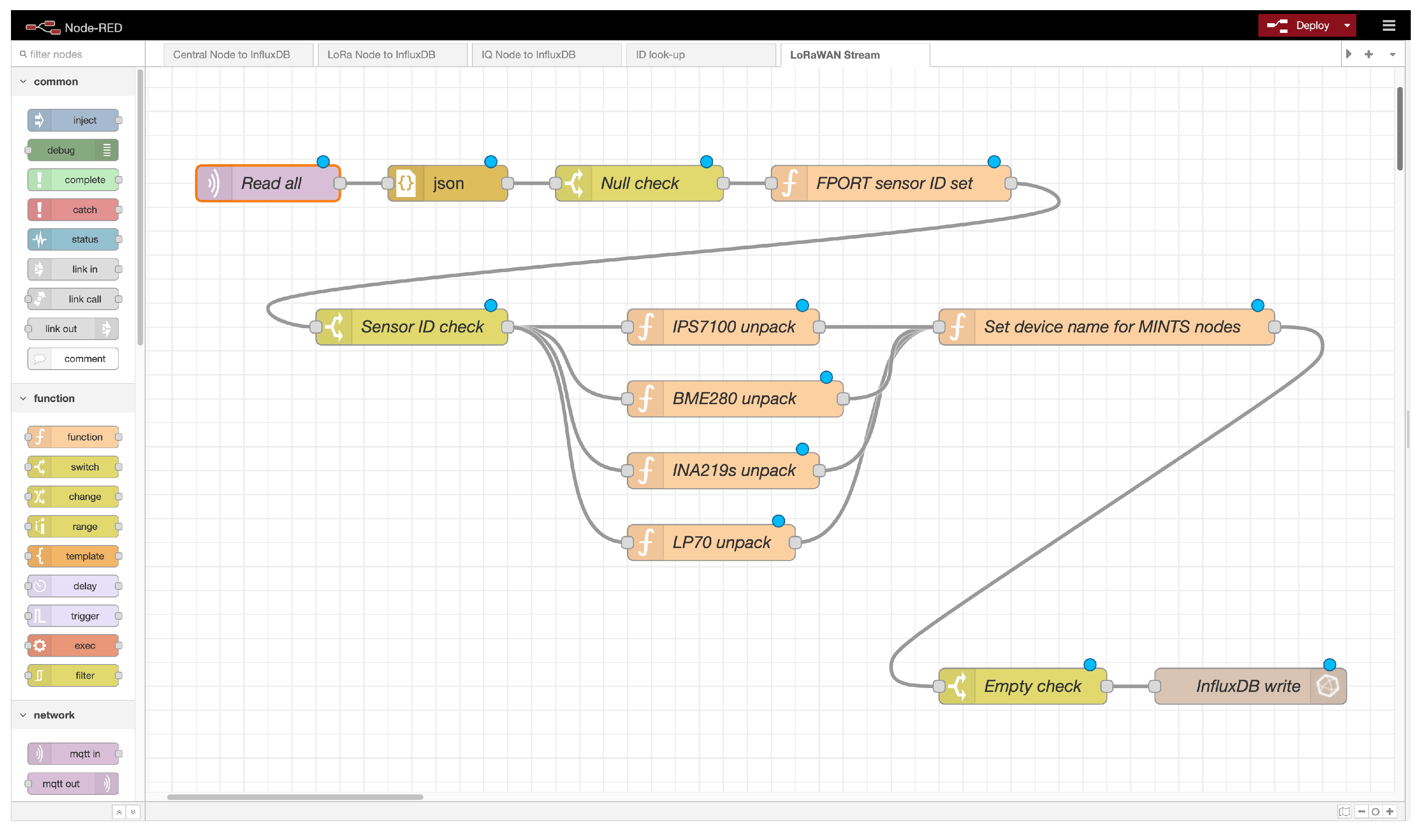
Figure 7.
InfluxDB Data Explorer: A sample query for is generated to select pm2.5 data from multiple LoRaWAN Nodes
Figure 7.
InfluxDB Data Explorer: A sample query for is generated to select pm2.5 data from multiple LoRaWAN Nodes
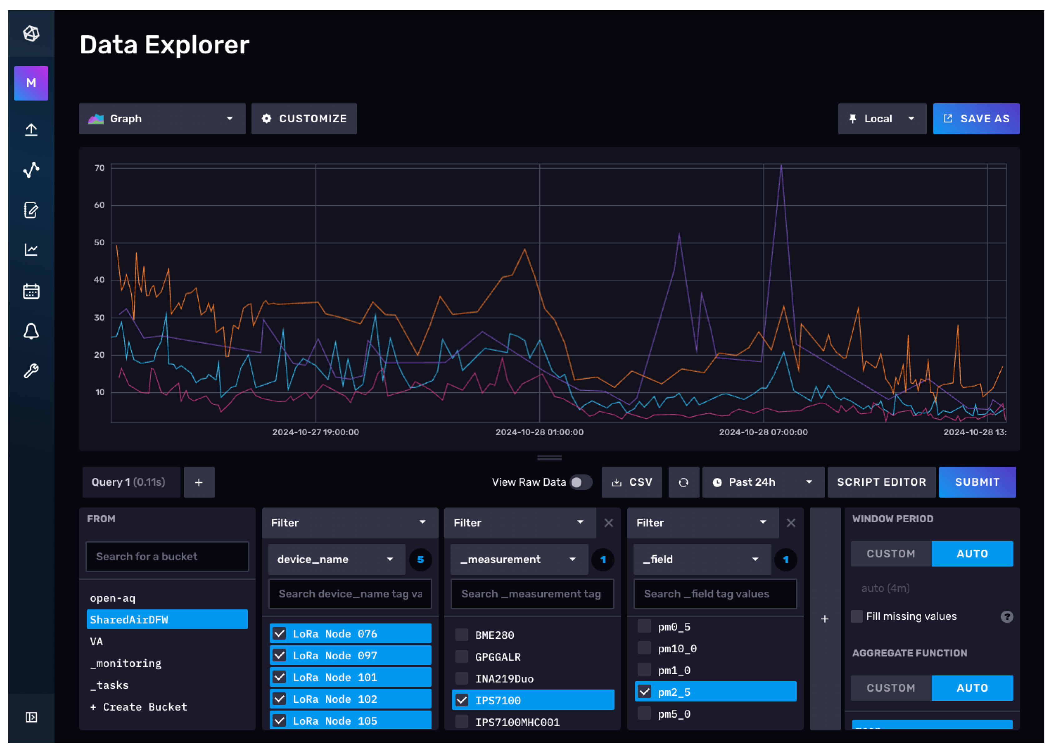
Figure 8.
Grafana Dashboard: This dashboard presents real-time data collected from a LoRaWAN sensor at UT Dallas, Richardson, for the week of October 14th to October 20th, 2024. First Row: The left panel displays particle counts categorized by size, the middle panel shows the most recent particle counts across size bins ranging from to , and the right panel indicates the sensor’s geographical location on a map. Second Row: The left panel presents a time series of particulate matter concentrations ranging from to , while the middle panel shows the most recent readings for particulate matter concentrations within the same range. The right panel presents the latest measurements of atmospheric temperature, pressure, humidity, dew point, solar voltage, solar power, battery voltage, and battery power. Third Row: A time series of climate data encompassing atmospheric temperature, pressure, humidity, and dew point. Fourth Row: A time series of power consumption data, outlining solar voltage, solar power, battery voltage, and battery power.
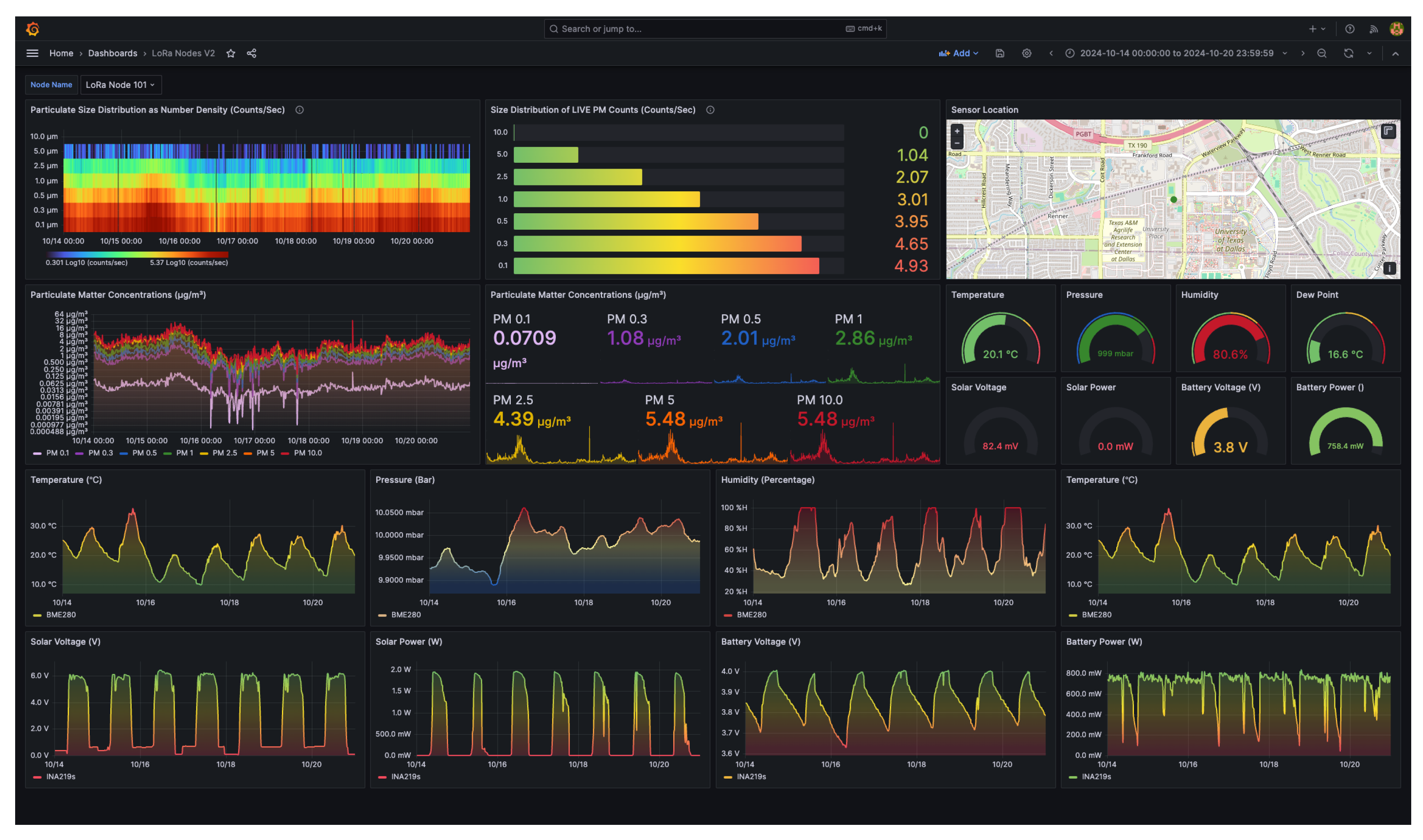
Figure 9.
Shared Air DFW Public Portal: Shared Air DFW is an initiative which operates out of the University of Texas at Dallas laboratories and is dedicated to deploying monitoring systems that have been designed and built by students at the university. Particulate matter data collected from these monitors, as well as information from EPA and DFW Purple Air monitors, are displayed in real time on a digital map accessible by anyone at www.sharedairdfw.com. The project is sponsored by the National Science Foundation, Earth Day Texas, the US Army, Downwinders at Risk, the City of Plano, and the US Environmental Protection Agency.
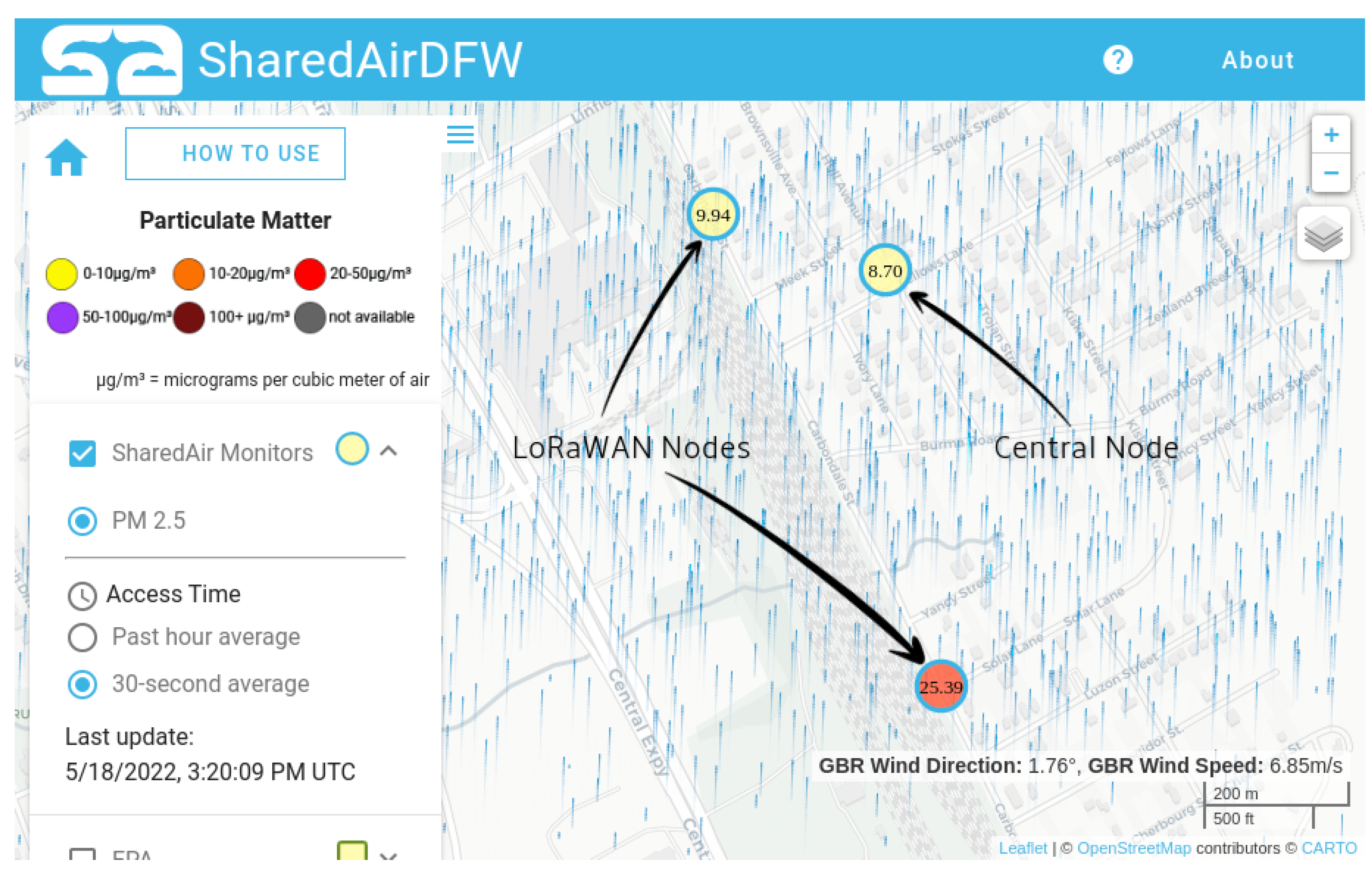
Figure 10.
Sensor Calibration Process: This figure presents the critical set points in the calibration process of the LoRaWAN Node. Before implementing Machine Learning Calibration, a humidity correction is applied to the input data collected from the IPS7100, utilizing the climate sensor (BME280). The machine learning model is trained using target data sourced from a Federal Equivalent Method (FEM) Beta Attenuation Monitor (BAM 1022) located in Fort Worth, Texas. This device is collocated with a MINTS sensor, and both systems continuously collect data 24/7 for eight months. Following the training of the machine learning model, the raw data from the IPS7100 and the BME280 sensors on the LoRaWAN nodes are utilized to produce more accurate data products. The blue arrows represents particulate matter data influenced by the IPS7100 and the green arrows represent the data coming from the climate sensor (BME280). The red arrow represent the particulate matter data provided by the Federal Equivalent Method (FEM) Beta Attenuation Monitor (BAM 1022). The purple arrow represents the deployment of the trained machine learning model.
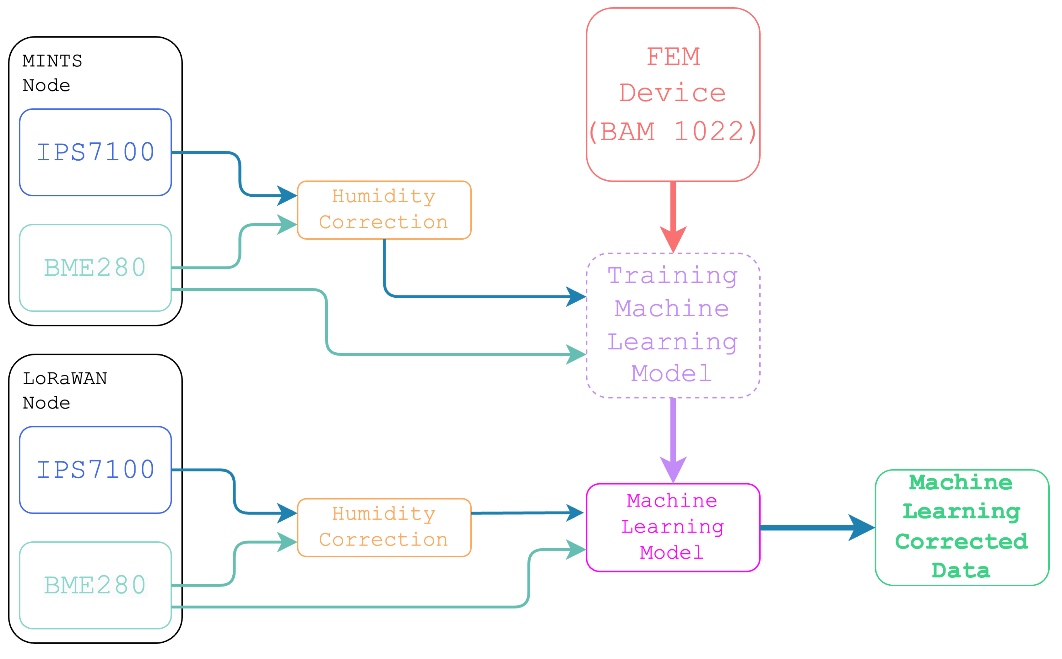
Figure 11.
This figure presents the results of a multivariate, non-linear, non-parametric machine learning regression for PM2.5. In Figure (a), the relationship between PM2.5 measurements from the BAM 1022 Beta Attenuation Mass Monitor (x-axis) and the PM2.5 levels predicted by the machine learning-calibrated IPS7100 instrument (y-axis) is shown. Training data is represented by blue circles, while green plus signs indicate independent validation data. The red line represents the ideal response. Figure (b) displays the quantile–quantile plot for the machine learning validation data. Here, the x-axis represents percentiles from the PM2.5 distribution of the BAM 1022, and the y-axis shows percentiles of the machine learning-calibrated PM2.5 distribution from the IPS7100. The dotted red line indicates the ideal response. The dotted red line shows the ideal response. Figure (c) illustrates the relative importance of input variables in the machine learning calibration of the low-cost setup, with the top three variables highlighted in green and subsequent variables in blue.
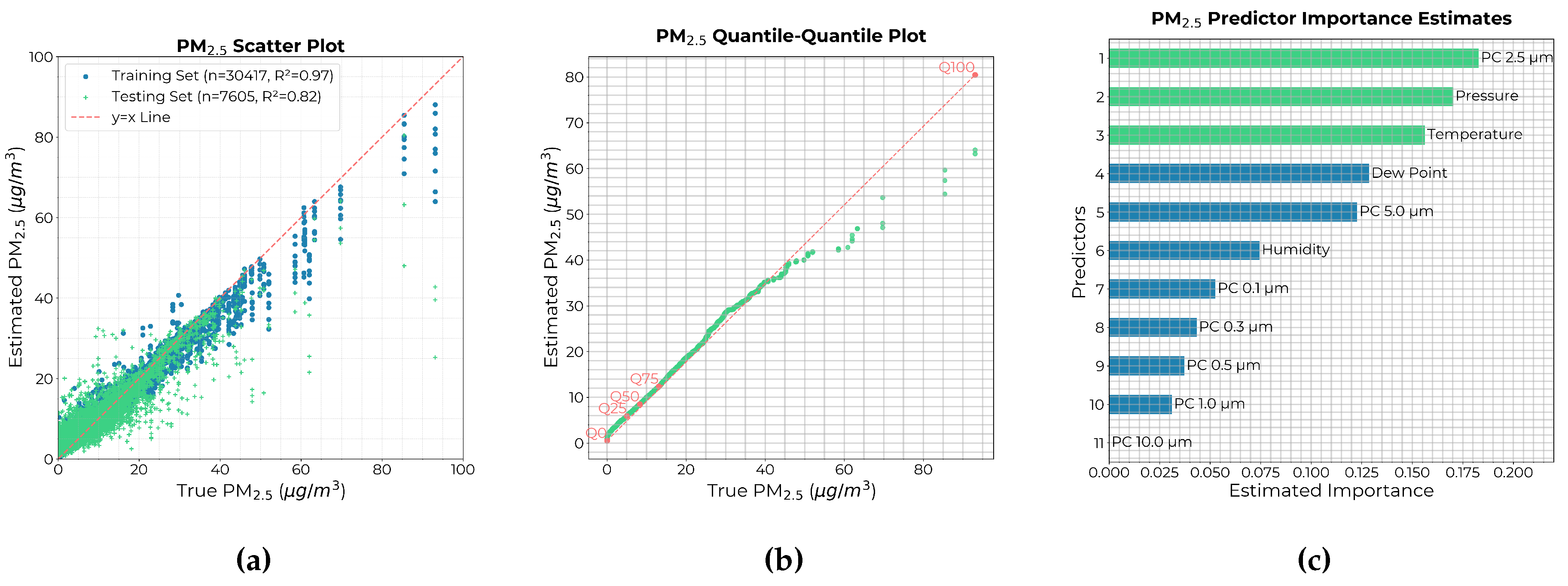
Figure 12.
Comparison of LoRaWAN Node PM2.5 Data: This figure presents PM2.5 data collected from a sensor at UT Dallas in Richardson for October 2024. The green time series represents the raw PM2.5 data from the IPS7100 sensor on the LoRaWAN nodes. The blue time series shows humidity-corrected PM2.5 values, while the red time series depicts PM2.5 values corrected using the machine learning mode
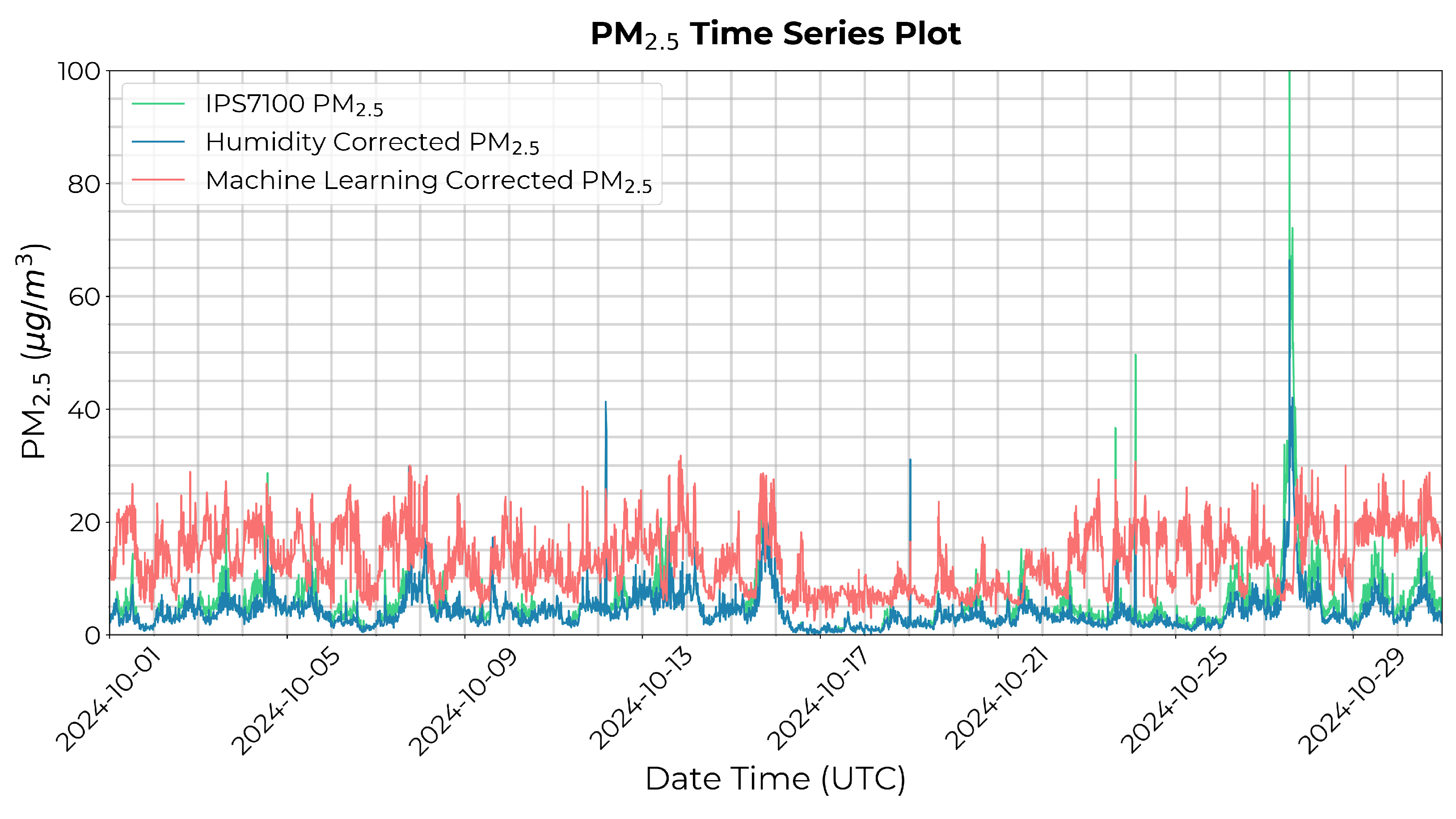
Table 2.
LoRaWAN Data Packets:
| Sensor ID | FPORT | Packet Size (Bytes) | Parameters Measured |
|---|---|---|---|
| IPS7100 | 15 | 56 | Standard Particulate Matter Mass fractions and Particulate Counts for Particulate Diameters 0.1, 0.3, 0.5, 1.0, 2.5, 5.0 and 10 . |
| BME280 | 21 | 12 | Climate readings of Atmospheric Temperature, Pressure and Humidity. |
| INA219s | 3 | 32 | Voltages, currents, and power readings for both the battery pack and solar panels. |
| LP70 | 5 | 55 | Longitude, latitude, altitude, as well as the UTC time stamps. |
In LoRaWAN Sensing systems, the Port field (FPort) is commonly used to differentiate between different types of messages. To distinguish between the sensors used, we use the FPort field. Although the current infrastructure only uses four specific sensors, the sensing system is designed to accommodate multiple sensors. In the table are the fields identifying each sensor, the packet sizes associated with the LoRaWAN payload, and the specific measurements made for each sensor.
Disclaimer/Publisher’s Note: The statements, opinions and data contained in all publications are solely those of the individual author(s) and contributor(s) and not of MDPI and/or the editor(s). MDPI and/or the editor(s) disclaim responsibility for any injury to people or property resulting from any ideas, methods, instructions or products referred to in the content. |
© 2024 by the authors. Licensee MDPI, Basel, Switzerland. This article is an open access article distributed under the terms and conditions of the Creative Commons Attribution (CC BY) license (http://creativecommons.org/licenses/by/4.0/).
Copyright: This open access article is published under a Creative Commons CC BY 4.0 license, which permit the free download, distribution, and reuse, provided that the author and preprint are cited in any reuse.


