
Submitted:
09 April 2025
Posted:
10 April 2025
You are already at the latest version
Abstract
Quaternions are used in various applications, especially in those where it is necessary to model and represent rotational movements, both in the plane and in space, such as in the modeling of the movements of robots and mechanisms. In this article, a methodology to model the rigid rotations of coupled bodies by means of unit quaternions is presented. Two parallel robots were modeled: a planar RRR robot and a spatial motion PRRS robot using the proposed methodology. Inverse kinematic problems were formulated for both models. The planar RRR robot model generated a system of 21 nonlinear equations and 18 unknowns, and a system of 36 nonlinear equations and 33 unknowns for the case of space robot PRRS; both systems of equations were of the polynomial algebraic type. The systems of equations were solved using the Broyden-Fletcher-Goldfarb-Shanno nonlinear programming algorithm and Mathematica V12 symbolic computation software. The modeling methodology and the algebra of unitary quaternions allowed the systematic study of the movements of both robots and the generation of mathematical models clearly and functionally.
Keywords:
Robotics
; quaternions
; kinematics
; parallel mechanisms
1. Introduction
The kinematic analysis of parallel kinematic machines is a challenging field since such machines are complex multi-body systems involving at least one pair of closed kinematic loops [1]. There are important differences between serial and parallel configuration robots, for example, the latter due to their robust structure, higher load capacity, versatility and excellent positioning accuracy [2].
In fact, in industrial automation, parallel manipulators have been considered an alternative to traditional automation to achieve a high load capacity, intelligent dynamic performance, and precise positioning that provide higher quality and more economical processes [3]. The main drawbacks of parallel robots are their small workspace and the singularities that can appear within the latter [2].
Parallel robots are currently used in various applications such as machining operations [4], additive manufacturing for construction [5], and dimensional metrology [6]. This type of robot is also used for medical operations [7] and in rehabilitation [8], as well as in flight simulators [9] and in telescope mechanisms [10], among others.
For the kinematic modeling of parallel robots, there are several mathematical methods and tools; the following is a summary. Homogeneous matrices and Denavit-Hartenberg parameters are regularly used for the kinematic modeling of this type of robot [11,12]. Also, geometrical methods have been used to study the planar motion of parallel-type robots [13,14] and their singularities [15]. Screw theory is also used in the modeling of parallel robots [16,17]. Complex number algebra [18] and quaternions [19,20] are used to model robot rotations in the plane and in space, respectively. Other versions of quaternions, such as dual representations, are also applied to the modeling of parallel robots [21,22].
While each mathematical tool and modeling method used to study parallel robots has its advantages and disadvantages, quaternions stand out due to their compact notation and ease of composition, and they are more efficient than matrix methods, involving fewer algebraic operations and, hence less computational storage. In fact, the performance of dual quaternions has been shown to improve by 30-40% in forwarding kinematics over conventional homogeneous transformation matrices [23]. These and other important features of quaternions and their representations make them ideal for modeling parallel robots. Recently, a PUMA-type robot has been modeled with the algebra of quaternions [24]. In this work, the systematization of the quaternions developed in 1990 at INRIA France [25,26] was applied. The results showed that it was possible to model the rotations of the links of an open chain robot clearly and systematically, performing all the operations in the vector space of quaternions avoiding the use of trigonometric relations during modeling. The PUMA robot was modeled using sequences of rotations and the numerical solution of the mathematical model associated with the inverse kinematics was obtained with the Newton-Raphson method.
In other works, quaternions have been applied to the analysis and synthesis of parallel robots, for example, in [27] the kinematic synthesis problem of a planar parallel robot of the RPR type was modeled using planar quaternions. The generated model allowed to achieve any desired configuration and the definition of the problem in the space of planar quaternions resulted in a definition of the work space of the parallel manipulator as the intersection of quadratic equations. In another study, the modes of operation and transition configurations of the parallel cylindrical mechanism 1-RPU-2-UPU were analyzed [28]. In that study, a reconfiguration analysis of a parallel manipulator was performed and the constraint equations were modeled using Euler parameter quaternion. Liu et al. [29] proposed an analytical algorithm using unitary quaternions to model the direct kinematics of a 6-UPS parallel robot with an additional displacement sensor mounted at the top and bottom platform centers ((6+1)-UPS). Birlescu et al [30] proposed a mathematical method to redefine motion parameterizations based on the joint space representation of parallel robots. The mathematical models were developed using dual quaternions, and the main feature of the model was that, instead of directly studying the motion of the moving platform, the joint space of the mechanism was analyzed by eliminating the study parameters. Finally, Liu et al. [31] analyzed the modes of operation and corresponding motion characteristics of low-mobility parallel mechanisms using unitary dual quaternions.
On the other hand, many mathematical models related to robot motions and mechanisms consider the unitary norm of quaternions which implies that the systems of equations are nonlinear. To solve this type of problem, the Newton-Raphson method is commonly used [24]. Quasi-Newton methods and the Davidon-Fletcher-Powell (DFP) algorithm have also been used to solve mathematical models of robots and mechanisms. For example, in [32] the DFP algorithm was applied to determine the numerical solution and optimization of parasitic motions of a 3 DOF parallel robot. There are several variants of the quasi-Newton methods and in all of them the idea is to consider the Hessian matrix in the quadratic model. The Broyden-Fletcher-Goldfarb-Shanno (BFGS) method is a variant of the DFP method and was used by Kashyap and Parhi (Kumar; Dayal) [33] to solve a path planning problem for a humanoid robot. In turn, Xie et al. [34], used the BFGS algorithm, the Newton-Raphson method and the Levenberg-Marquardt algorithm to compute the inverse kinematic problem for a 7 DOF open-chain robot.
On the other hand, the PRRS type and the RRR planar robot stand out from the existing set of parallel spatial and planar robots. The PRRS space robot has been studied in [35] where its design was developed using structural synthesis modeling and degrees of freedom analysis. On the other hand, the RRR planar robot, due to its simple configuration, has been used to test different kinematic and dynamic modeling [36,37]. In other works, this robot was used to develop artificial intelligence tests [38,39] and to test different control models [40,41], as well as for the study and analysis of singularities [42,43].
This paper describes and applies a novel methodology using unitary quaternions for the study of the motions of parallel PRRS and RRR type robots. This methodological proposal is a continuation of the modeling method described in [24] and aims to extend the applications of the quaternion systematization developed by Reyes [25,26] to other types of robots, in this case, to the study of parallel robots. With the mathematical models generated for each robot analyzed, inverse kinematic problems were formulated. These problems were solved using the formal calculation platform Mathematica V12. The novelties of this work with respect to the results presented in [24], are: 1) for the modeling of the robots under study two configurations are not considered, 2) the mathematical models generated are non-square and non-linear and 3) the solution method used was BFGS optimization method [44,45,46]. Although there are already several methodologies that take quaternions into account as the basis for modeling robot motions [24,47,48,49,50,51,52], the method proposed in this paper is general and can be applied to model parallel robots in the plane and in space.
2. Materials and Methods
In this section a summary of the theoretical framework of Quaternion algebra and the methodology to systematize rotations using unitary quaternions is presented. In addition, modeling of RRR and PRRS robots of parallel configuration is developed. The inverse kinematic problem is formulated for both robots and the BFGS optimization method with which the generated mathematical models were solved is described.
2.1. Preliminaries of the Algebra of Quaternions
A systematic way of constructing the algebra of quaternions with a modern linear algebra focus is presented in [24,25,26]. Let the set 4, on which the binary operations are defined ⊕:4×4®4 and ∗: 4× 4®4 be expressed:
i) (a,b,c,d) ⊕ (α,β,γ,δ) = (a+α, b+β , c+γ , d+δ) (1)
ii) (a,b,c,d) ∗ (α,β,γ,δ) = (aα − bβ − cγ − dδ, aβ + bα + cδ − dγ, aγ − bδ + cα + dβ, aδ + bγ-cβ + dα ), ∀ (a,b,c,d), (α,β,γ,δ) ∈ 4
The pairs (4,⊕) and (4,∗) form a commutative additive group and a non-commutative multiplicative group, respectively. The triple (4,⊕,∗) forms a non-commutative field. This is:
The operation ∗:4×4®4 is associative, since:
- i)
- p∗(q∗s) = (p∗q)∗s; ∀ p, q, s∈4 (2)
- ii)
- The element 1 = (1,0,0,0) ∈ 4 is such that: 1∗p=p∗1=p, ∀p∈4. This element is known as the neutral element of the multiplication in 4.
- iii)
- iii) ∀p∈4, p ≠ (0,0,0,0); p’∈4 such that p∗p’ = 1. The element p’ is called the multiplicative inverse of the quaternion p.
- iv)
- iv) The operation ∗:4×4®4 is not commutative. This is:
- v)
- p∗q ≠ q∗p
- vi)
- The following distributive properties are satisfied:
a) (p⊕q)∗s = p∗s ⊕ q∗s (3)
b) p∗(q⊕s) = p∗q ⊕ p∗s, ∀p, q, s∈4
On the other hand, the operation ∙:×4®4 is defined by:
α∙(a,b,c,d) = (αa,αb,αc,αd), ∀(a,b,c,d)∈4, α∈ (4)
It is a scalar product on 4, so the term (4,⊕,∙) is a real vector space. The transformation <∙,∙>:4× 4®, is defined by:
(5)
It is an inner product in 4 and, therefore, the structure Q=(4,⊕,∗,∙,<∙,∙>) is a real vector space with inner product, and the norm associated with this inner product is the following:
||p|| = <p,p>1/2 = (p02+p12+p22 +p32) 1/2 (6)
For which the structure Q=(4,⊕,∗,∙, |∙|) is a normed space which will be called the vector space of quaternions, and its elements will be called quaternions [25].
It is possible to represent a quaternion as the sum of a real quaternion and a vector quaternion. Let the following subsets be:
Qr = {(a,0,0,0) : a∈}⊂Q, (7)
Qv = {(0,b,c,d) : b,c,d∈}⊂Q
The transformations are defined by:
Tr(a,0,0,0) = a ∀(a,0,0,0)∈Qr (8)
Tv(0,b,c,d) = (b,c,d) ∀(0,b,c,d)∈Qv
are isomorphic, and therefore, if p=(a,b,c,d)∈Q, then:
p = (a)
(b, c, d) (9)
In a similar way to the algebra of complex numbers, a conjugate quaternion can be defined as follows:
(10)
given p=(p0, p1, p2, p3) and q=(q0, q1, q2, q3) ∈Q, then:
- 1)
- (11)
- 2)
- 3)
2.2. Parametric Representation of Rotations of a Rigid Body
Let ρ(p,•):Q→Q, p∈Q be a linear transformation defined by:
(12)
This function is a rotation that preserves the inner product, the norm, and the angle [25]. The transformation ρ(p,∙):Q→Q, is linear, orthogonal and ρ(p, q)∈Qv, by all q∈Qv. Let θ∈[0, nπ], n∈+, w∈Qv, ||w||=1; then, the quaternion p∈Q, with p0∈−{0} and pv = ± sinθw, is such that, ρ(p, w)=w, where p0 satisfies the equation:
4 p04 − 4 p02 ||p||2cosθ − ||p||4sin2θ = 0 (13)
The quaternion p represents a rotation of angle θ∈[0, nπ], with axis w∈Qv, giving:
p0 = ||p|| cos(θ/2), pv = ± ||p||sin(θ/2)w (14)
In general, the norm of p can be arbitrary. Unit quaternions will be used in this article; that is, ||p||=1, so expression (14) reduces to:
p0 = cos(θ/2), pv = ± sin(θ/2)w (15)
2.3. Kinematic Modeling of Coupled Bodies
This section presents the methodology for modeling the rotations of coupled rigid multi bodies using the algebra of quaternions [25], to later be applied in the analysis of the movement of RRR parallel planar and PRRS spatial robots. The modeling process involves a representation of a rigid body to determine the position of a point on it with respect to an inertial reference system. To achieve a systematic representation of the rotations, it is necessary to define functions that allow transforming vectors defined in 3 to the Q space and vice versa.
2.3.1. Isomorphism of the Vectors of 3 to the Vector Space Q
It is possible to define a function Tv: Qv→3, between the subspace of the vector quaternion Qv and the vector space 3, according to expressions (8). This is:
Tv(0,b,c,d) = (b,c,d); ∀(0,b,c,d) ∈Qv
Subsequently, the transformations described by expressions (8) are isomorphic; then there is an inverse transformation : 3→Qv, such that:
(b,c,d) = (0,b,c,d); ∀(b,c,d) ∈3 (16)
Therefore, any vector of 3 can be considered an element of the vector space of quaternions [25]. Thus, by applying the proposed isomorphism of expression (16) to the canonical basis in 3 defined by:
B= {(1,0,0), (0,1,0), (0,0,1)} (17)
the following is obtained:
e1 = (1,0,0) = (0,1,0,0) (18)
e2 = (0,1,0) = (0,0,1,0)
e3 = (0,0,1) = (0,0,0,1)
Here, {ej }∈4 and j=0,1,2,3, are vectors of the canonical base of 4, which is completed with the vector e0=(1,0,0,0). It is important to highlight that the previous isomorphism allows us to work with the elements of 3 using the algebraic properties of the space of the quaternions Q.
2.3.2. Rotation of a Cartesian Frame of Reference
This section presents the procedure to apply a rigid rotation with the algebra of quaternions. The linear transformation ρ(p,•):Q→Q, with p=(p0,p1,p2,p3) fixed, described in expression (12) is a rotation [24,25]. The components of rotation are described by expressions (15), where θ∈[0, nπ] is the angle of rotation and w=(w1,w2,w3), w∈Qv, is the axis of rotation. When considering quaternions of unitary norm, the expression (12) takes the following form:
(19)
Expression (19) is very useful in kinematics applications when one reference system has to be associated with another, relating it by means of rotations of the base that forms each of these systems. To characterize a rotation between bases, an inertial base ej∈3 is established, for j=1,2,3, and a local base ejn∈3, attached to a rigid body and rotating with it. The orientation of the body is defined by the orientation of the local base ejn.
We also establish the bases ej ∈4 and ejn ∈4 which are associated with the bases ej∈3 and ejn ∈3 which will allow us to perform operations in the vector space of quaternions. These bases are related to each other by the transformations ej = Tv(ej) and ejn = Tv(ejn). To determine the relationships between these bases, unit vectors e1, e2, e3 in Figure 1, can be seen directed along the coordinate axes x, y, z, respectively. We also have unit vectors e1n, e2n, e3n, directed along the coordinate axes xn, yn, zn, attached to the rigid body. At the beginning of the movement, both bases ej and ejn coincide.
For any rotational movement of the body shown in Figure 1, there is a general quaternion p = (p0, p1, p2, p3) which defines the final orientation of the body and is expressed as follows:
(20)
For the case where the orientation of a rigid body in three-dimensional space is defined by three rotations in the axes x, y, z, (although they can be defined in other axes) [53], expression (20) must be put in terms of the composition of three rotating quaternions p = p1*p2*p3, where p1 = (p10, p11, 0, 0), p2 = (p20, 0, p22, 0), and p3 = (p30, 0, 0, p33). The order of composition of the quaternions is explained in Appendix A.
2.3.3. Configuration of Coupled Bodies
The objective of this section is to determine the relationships between the bases associated with coupled bodies. According to Figure 2, the links of a kinematic chain are represented by the vectors R1, R2∈3. The link R1 is joined to the base by means of a rotational joint at point A. Link R2 is joined to R1 by means of a universal joint at point B. This allows modeling a general movement of the articulated links which can then be applied to model mechanisms. To start the modeling process, a global reference system is first defined ej and local reference systems ejn, j=1,2,3 over the links. The position vector RP and the vectors R1, R2 associated with the links are represented in 4 as follows:
RP = (0,x,y,z) (21)
R1 = r1 e11
R2 = r2 e12
Here, R1, R2, RP ∈4, and r1, r2∈+ are the length of the links.
The modeling process is as follows:
The first step consists in determining the coordinates of the point "p" by means of the vector RP and considering vectors R1 and R2. The vector RP defines the position of the final end of the kinematic chain with respect to the global base ej. This vector can be written as follows:
RP = R1 ⊕ R2 = r1 e11 ⊕ r2 e12 (22)
The second step consists in transforming the elements of the bases e11 and e12 to the canonical base ej to obtain the vector RP referenced to the global base. The cases of spatial and planar motion will be considered.
1. In the case of spatial movement, this is modeled through the composition of relative movements, and the bases are defined as follows:
e11 = ρ(p1, e1) (23)
e12 = ρ(q,e1)
where,
q = p1*p2*p3 (24)
and where:
p1 = (p10, 0, 0, p13) (25)
p2 = (p20, 0, 0, p23)
p3 = (p30, 0, p32, 0)
2. For the case of planar movement, p2=0, p1 and p3 have a rotation axis in the z axis. This movement can be modeled by the composition of relative movements or also by mean absolute movements. For relative motion, the bases are defined as:
e11 = ρ(p1, e1) (26)
e12 = ρ(q,e1)
Here,
q = p1*p3 (27)
where:
p1 = (p10, 0, 0, p13) (28)
p3 = (p30, 0, 0, p33)
For absolute motion, the bases are defined as follows:
e11 = ρ(p1, e1) (29)
e12 = ρ(p3,e1)
The last step consists in obtaining a general expression of equation (22) and this is achieved by substituting, for the case of spatial movement, equations (23) in equation (22). This is:
RP = r1 ρ(p1, e1) ⊕ r2 ρ(q,e1) (30)
=
2.4. Modeling of a RRR Planar Parallel Robot
This section presents the modeling of a RRR planar robot using the results of the previous sections. The formal definition of a parallel robot is as follows: A parallel robot is made up of an end-effector with n degrees of freedom, and of a fixed base, linked together by at least two independent kinematic chains. Motion is originated by n single actuators [54].
This definition is important because it has implications for robot modeling, which consists of building a mathematical model through which it is possible to formulate the inverse kinematic problem associated with a said robot, which is shown in Figure 3. The degrees of freedom of the kinematic chain shown in Figure 3 are obtained using the following expression [55]:
DOF = 3(L −1) − 2J1 – J2 (31)
Here, L is the number of links, J1 is the number of full joints, and J2 the number of semijoints. Therefore, for L=8, J1=9, and J2=0, the degrees of freedom of the studied mechanism is DOF =3.
The robot shown in Figure 3 consists of a mobile platform that moves freely along the work plane and six links, three of which are connected to three actuators which provide movement, and three coupling links.
The objective of the modeling is to pose the inverse kinematic problem associated with the robot configuration shown in Figure 3. This problem is formulated as follows:
"Given the coordinates of the centroid of the mobile platform and its angle with respect to the x-axis, find the angles of the driving and driven links that make up the robot."
To start the modeling, it is necessary to consider the definition of a parallel robot to build the equations that govern the inverse kinematic problem, decoupling each chain that composes it, and to study each separately. The parallel robot shown in Figure 3 consists of three independent kinematic chains. Each chain has an associated motor, drive link, driven link, and moving platform. The modeling process for the planar case and for each kinematic chain is as follows:
1) Locate a coordinate system (x, y) and the fixed inertial base.
2) Select a kinematic chain.
3) Associate vectors to each link of the selected kinematic chain.
4) Associate mobile bases for each rotation movement when going through the chain (Figure 4).
5) Construct the equation of position that locates the centroid of the platform with the origin (x, y).
6) Model the base rotations using expression (19).
7) Represent the position equation from step 5 in terms of quaternions.
8) Repeat the process for each of the remaining kinematic chains.
9) Formulate the inverse kinematic problem.
Figure 4.
Inertial base and mobile bases.
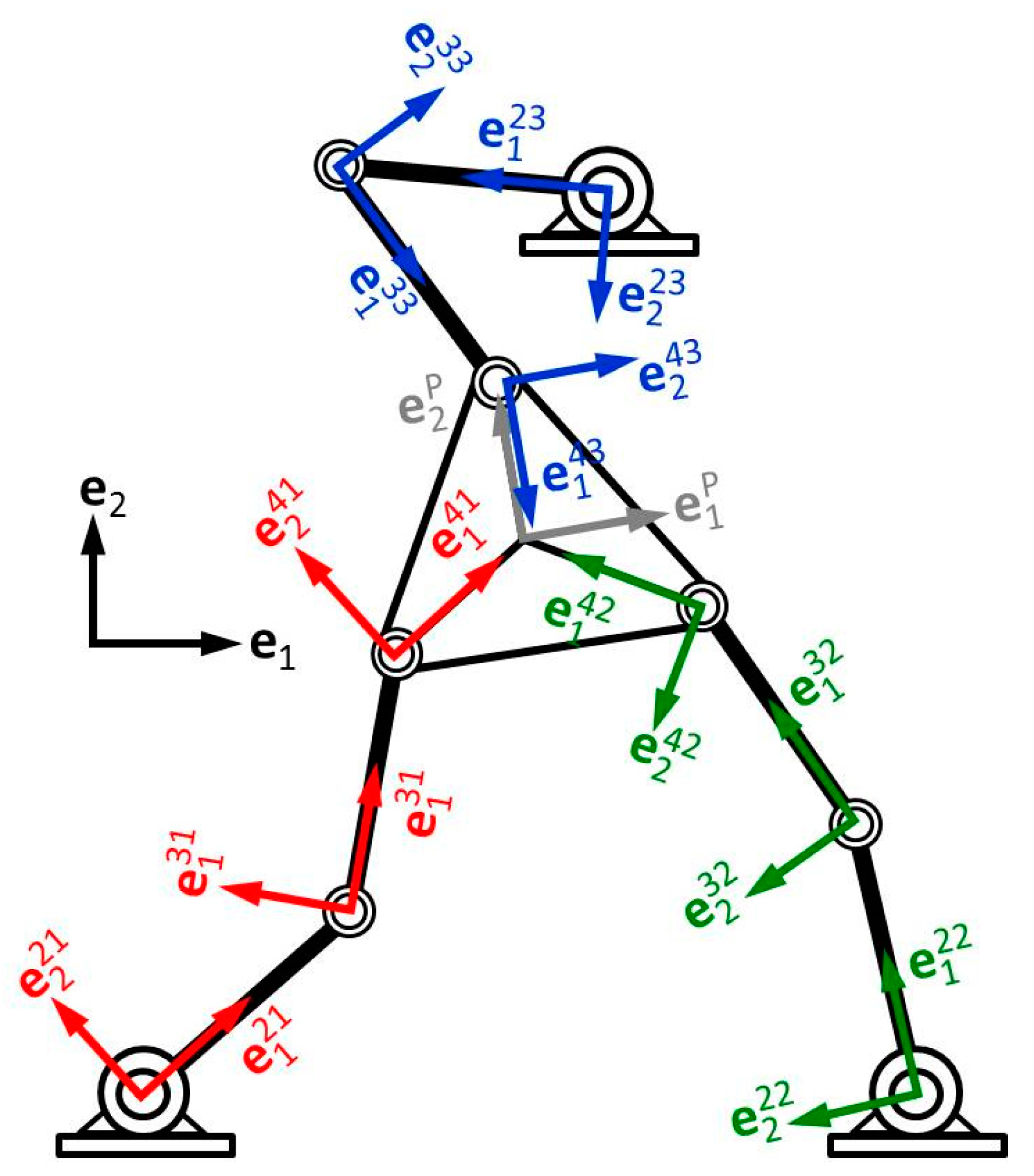
Figure 4 shows the inertial base and the moving bases associated with each link. Figure 5 shows the rotation angles of each link and of the mobile platform.
2.4.1. Loop Equations
In this section, the loop equations related to each kinematic chain associated with the robot under study are generated. Each link is represented by the vectors R2i, R3i, R4i∈3 on which the mobile bases ej2i, ej3i and ej4i are defined. Therefore, the position vector RP∈3 that locates the platform centroid from the origin of the coordinates can be expressed in terms of the vector sum in 4 for the case of the kinematic chains that make up the robot in the following way:
R1i ⊕ R2i ⊕ R3i ⊕ R4i = RP (32)
Furthermore, by considering unitary quaternions to represent the rotations of each link that make up each chain, unitary norm equations are generated. This is:
||p2i||2 = 1 (33)
||p3i||2 = 1
||p4i||2 = 1
Each vector associated with the links can be represented in terms of its length and in the direction of a unitary vector, according to expressions (21), as follows:
R1i = (0, xi, yi, 0) (34)
R2i = r2i e12i
R3i = r3i e13i
R4i = r4i e14i
RP = (0, xP, yP, 0)
where i=1,2,3, in addition to r2i, r3i and r4i are the lengths of the links. Each mobile base represents a rotation of the inertial base ej. Such rotations can be expressed in terms of relative quaternions. This is:
e12i = ρ(q2i, e1); q2i = p2i (35)
e13i = ρ(q3i,e1); q3i = p2i*p3i
e14i = ρ(q4i, e1); q4i = p2i*p3i*p4i
ej5i = ρ(q5i, ej); q5i = p2i*p3i*p4i*p5i
ejP = ρ(qP, ej); qP = pP
or, in terms of absolute quaternions:
e12i = ρ(p2i, e1) (36)
e13i = ρ(p3i,e1)
e14i = ρ(p4i, e1)
e15i = ρ(s5i, e1); s5i = p4i*p5i
where:
p2i = (p20i, 0, 0, p23i) (37)
p3i = (p30i, 0, 0, p33i)
p4i = (p40i, 0, 0, p43i)
p5i = (c(βi/2), 0, 0, s(βi/2))
pP = (c(θP/2), 0, 0, s(θP/2))
The quaternions p2i, p3i, and p4i, are associated with the angles θ2i, θ3i, and θ4i. In addition, the quaternions p2i, p3i, and p4i, allow the rotations of the first, second and third link of each kinematic chain to be carried out.
2.4.2. Platform Orientation Equation
The mobile platform of the robot under study can be oriented in each movement. The orientation equation is obtained by considering the following equality:
ej5i = ejP (38)
For the case of relative quaternions, we have:
ρ(q5i, ej) = ρ(qP, ej) (39)
if and only if:
q5i = qP (40)
Finally,
p2i*p3i*p4i*p5i = pP (41)
2.4.3. Formulation of the Inverse Kinematic Problem of the RRR Planar Parallel Robot
In this section, a problem of fundamental importance for rigid body kinematics is formulated: the inverse problem, which is associated with the configuration of the planar parallel robot shown in Figure 3. The formulation of said problem is as follows:
“Once the coordinates of the position vector RP and the angleθP are known, which respectively define the position of the origin and the orientation of the base ejP on the mobile platform, determine the angles (θ2i,θ3i,θ4i) of the chains kinematics associated with the quaternions p2i, p3i, p4i, such that equations (32), (33) and (41) are satisfied.”
The formulation of the inverse problem of the RRR robot modeled with unitary quaternions generates a system of 21 nonlinear equations with 18 unknowns of the algebraic type.
For each string, equation (32) generates two algebraic equations in x and y, equations (33) represent three unitary norm equations, and expression (41) generates two other algebraic equations, so adding them together, 21 equations are obtained. Similarly, for each chain, there are six unknowns, which are the components of the quaternions p2i, p3i, and p4i; that is (p2i0, p2i3, p3i0, p3i3, p4i0, p4i3) and, therefore, there are 18 unknowns.
Once the quaternions p2i, p3i, and p4i, have been calculated, the associated angles (θ2i, θ3i, θ4i) can be determined using the following relationships:
θ2i = 2 tan-1(p2i3/p2i0) (42)
θ3i = 2 tan-1(p3i3/ p3i0)
θ4i = 2 tan-1(p4i3/ p4i0)
2.5. Modeling of a PRRS Spatial Parallel Robot
The objective in this section is to apply the unitary quaternion modeling methodology described in section 2.3.3 to study the motions of a PRRS-type spatial parallel robot [35]; that is, the robot has prismatic (P), rotational (R) and spherical (S) joints, like the one shown in Figure 6. Said robot consists of three independent kinematic chains and a mobile platform. The links that connect the robot with the bed or ground of the system have associated prismatic joints (P) that move along the axes of a Cartesian system. Each chain has two links that are articulated by means of rotational joints (R) and finally the connection of the links with the mobile platform is by means of a spherical joint (Figure 6).
The objective of the study is to determine a mathematical model that allows formulating the inverse kinematic problem associated with the configuration of the robot.
2.5.1. Loop Equations
According to Figure 6, to locate the coordinates of point "P" located at the centroid of the mobile platform from the origin of coordinates of the entire system, the closed-loop equations must be formulated. These expressions are obtained by means of the following vector equation:
R1xi ⊕ R1yi ⊕ R2i ⊕ R3i ⊕ R4i = RP (43)
When considering unitary quaternions to model the rotations of the links with R- and S-type connections that make up each chain, unitary norm equations are generated. This is:
||p4i||2 = 1 (44)
||p5i||2 = 1
||p6i||2 = 1
||p7i||2 = 1
||p8i||2 = 1
The vectors associated with the links that make up the robot can be put in the function of the local bases which are shown in Figure 7. That is
R1xi = xi e11i (45)
R1yi = yi e21i
R2i = r2i e22i
R3i = r3i e23i
R4i = r4i e14i
RP = (0, xP, yP, zP)
The mobile bases (see Figure 7) associated with the links can be written in terms of unitary quaternions and in terms of the canonical basis as follows:
ej1i = ρ(q1i, e1); q1i = p1i*p2i*p3i (46)
e22i = ρ(q2i, e1); q2i = q1i*p4i
e23i = ρ(q3i,e1); q3i = q2i*p5i
e14i = ρ(q4i, e1); q4i = q3i*p6i*p7i*p8i
ej5i = ρ(q5i, ej); q5i = q4i*p9i
ejP = ρ(qP, ej) qP = pψ*pθ*pφ
The configurations of each quaternion in terms of the angles of rotation are (see Figure 8):
p1i = (c(β1i/2), 0, s(β1i/2), 0) (47)
p2i = (c(β2i/2), 0, 0, s(β2i/2))
p3i = (c(β3i/2), s(β3i/2), 0, 0)
p4i = (p40i, p41i, 0, 0)
p5i = (p50i, p51i, 0, 0)
p6i = (p60i, 0, 0, p63i)
p7i = (p70i, 0, p72i, 0)
p8i = (p80i, 0, 0, p83i)
p5i = (c(β5i/2), 0, 0, s(β5i/2))
pψ = (c(ψ/2), 0, 0, s(ψ/2))
pθ = (c(θ/2), 0, s(θ/2), 0)
pφ = (c(φ/2), 0, 0, s(φ/2))
Figure 7.
Inertial and mobile bases.
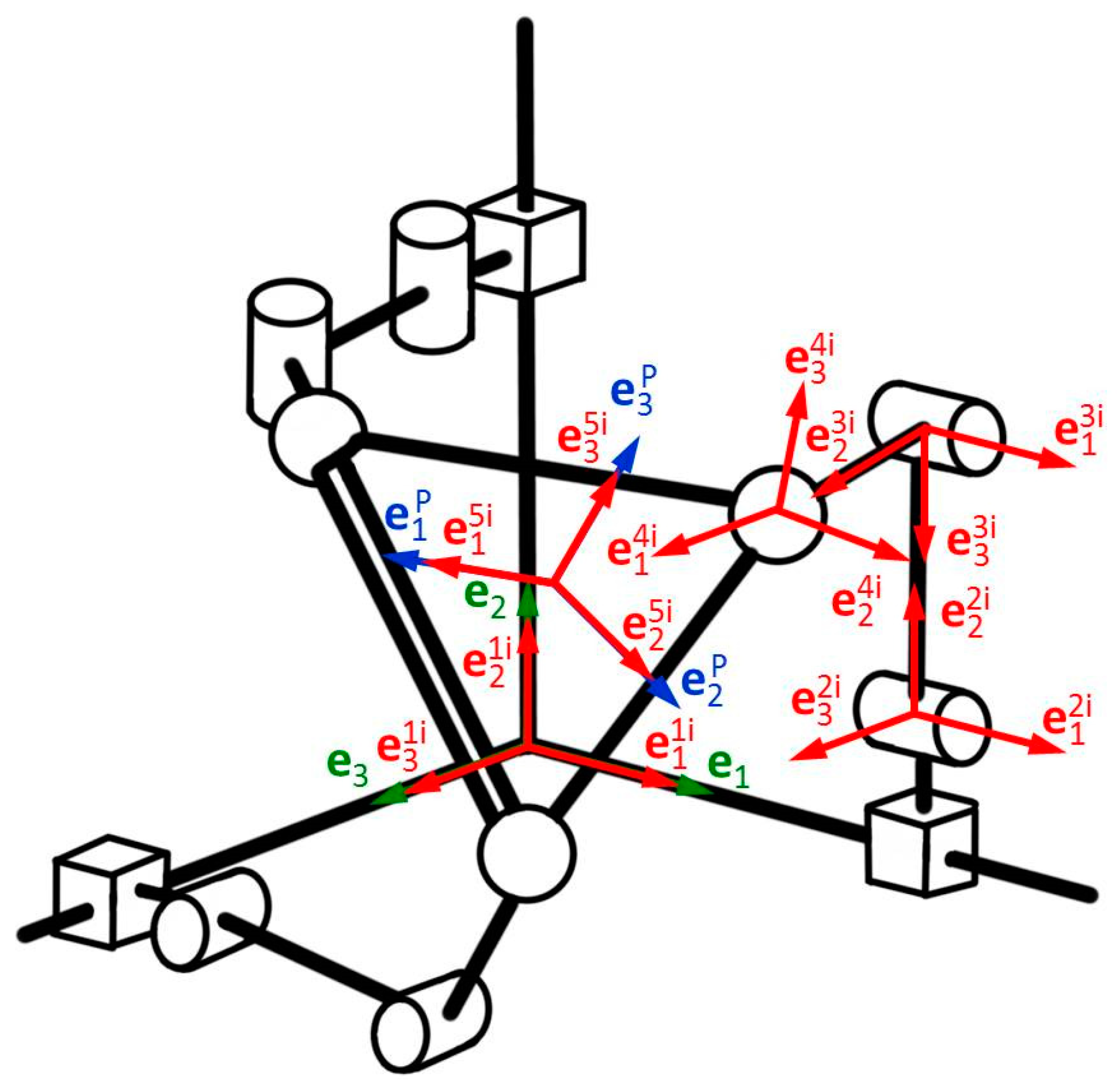
Figure 7 shows the inertial base and the moving bases associated with each link. Figure 8 shows the rotation angles of each link and of the mobile platform.
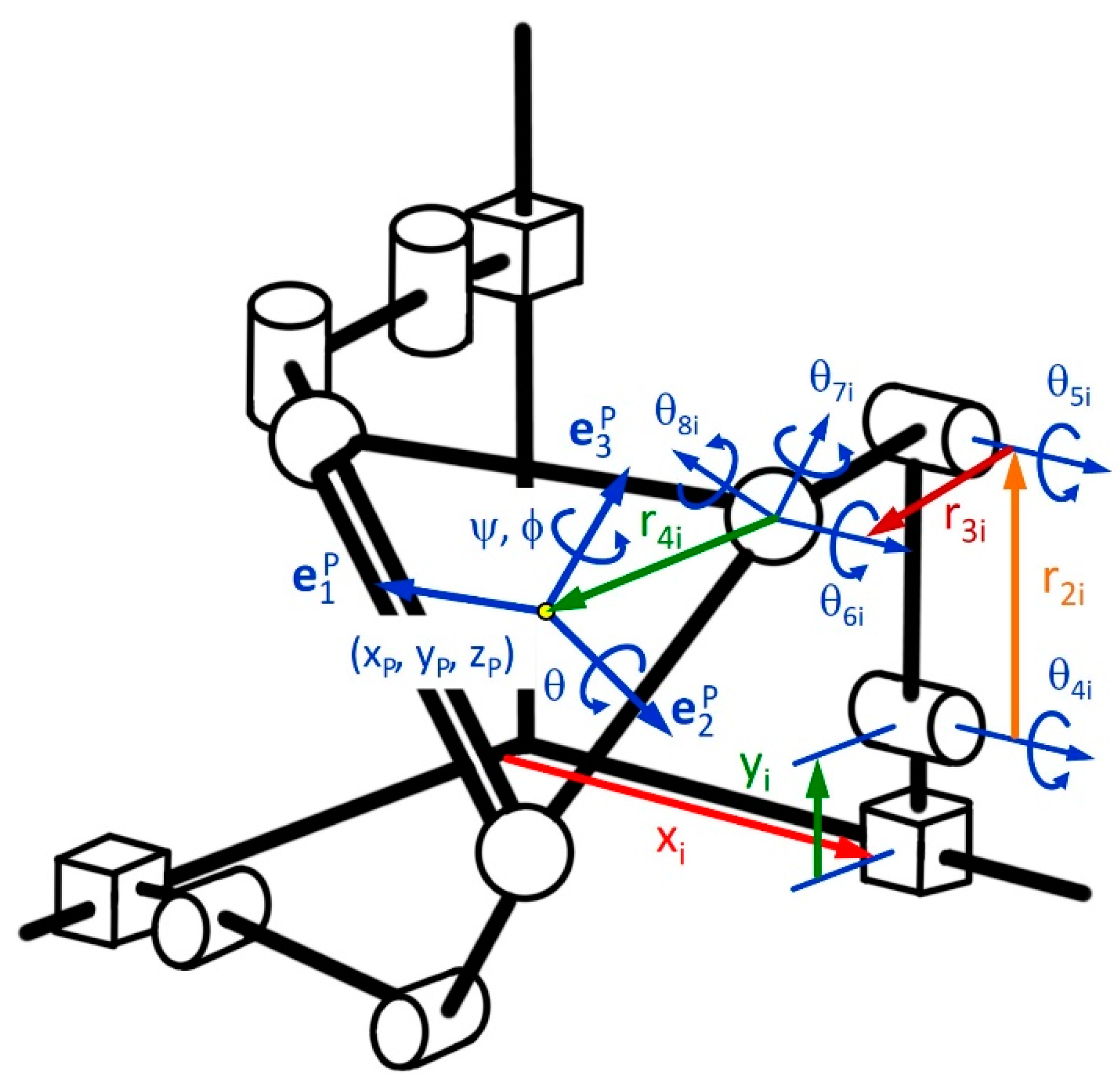
Figure 8.
Angles of the bases.
2.5.2. Equation of Platform Orientation
To complete the modeling of the robot under study, it is necessary to build the equations that allow defining the orientation of the mobile platform. This equation is obtained by considering the following equality:
ej5i = ejP (48)
Being
ρ(q5i, ej) = ρ(qP, ej) (49)
and,
q5i = qP (50)
then
p1i*p2i*p3i*p4i*p5i*p6i*p7i*p8i*p9i = pψ*pθ*pφ (51)
2.5.3. Formulation of the PRRS-Type Inverse Problem
In this section, the inverse kinematic problem associated with the configuration of the PRRS robot shown in Figure 6 is formulated. This formulation is as follows:
“Known the coordinates of the point “p” (RP) located in the centroid of the mobile platform, and the anglesψ,θ,φ, which respectively define the position of the origin and the orientation of the base ejP in the mobile platform, determine the magnitude xi and the angles (θ4i,θ5i,θ6i,θ7i,θ8i) of the kinematic chains associated with the quaternions p4i, p5i, p5i, p6i, p7i, p8i,, such that equations (43 ), (44) and (51), be satisfied.
The formulation of the inverse problem of the PRRS robot modeled with unitary quaternions generates a system of 36 nonlinear equations with 33 unknowns of the algebraic type.
For each string, equation (43) generates three algebraic equations in x, y, z, equations (44) represent five unitary norm equations, and expression (51) generates another four algebraic equations, so when added together 36 equations are obtained. In the same way for each chain, there are 11 unknowns, which are the components of the quaternions p4i, p5i, p5i, p6i, p7i y p8i, that is (p40i, p41i, p50i, p51i, p60i, p63i, p70i, p72i, p80i, p83i) and the displacement xi of the prismatic joint.
Once the quaternions p4i, p5i, p5i, p6i, p7i y p8i are calculated, the associated angles (θ4i, θ5i, θ6i, θ7i, θ8i) can be determined by means of the following relations:
θ4i = 2 tan-1(p41i/p4i0) (52)
θ5i = 2 tan-1(p51i/p50i)
θ6i = 2 tan-1(p63i/p60i)
θ7i = 2 tan-1(p72i/p70i)
θ8i = 2 tan-1(p83i/p80i)
2.6. Numerical Experimentation
In this section, the numerical experimentation for the solution of the inverse kinematic problems of both robots is presented. To solve the nonlinear and non-square systems of equations derived from the inverse problem statements, the BFGS nonlinear programming algorithm [46] was used.
The Davidon-Fletcher-Powell (DFP) method is a quasi-Newton method and is used to find the unconstrained minimum of a differentiable function “f” of several variables, and consists of generating successive approximations of the inverse of the Hessian of the function under study. The DFP method has been and remains a widely used gradient technique. The method tends to be robust; that is, it typically tends to perform well on a wide variety of practical problems and was first proposed by Davidon [56] and later reformulated by Fletcher and Powell [57]. A variant or improvement of the DFP is the BFGS algorithm [33,34], which is currently considered the most efficient of all Quasi-Newton update formulas, and is a computational iterative technique used to solve nonlinear optimization problems by using the first derivative and the Hessian matrix of the objective function [58]. The DFP update formula is bastantly effective, but it is outperformed by the BFGS formula [33,59]. In this paper we propose the objective functions associated with the position kinematics of each robot studied and use the BFGS algorithm which is automated in the Mathematica V12 formal computation library [46].
3. Results
This section presents the results obtained by solving the mathematical models of the robots studied in this work. An objective function and a trajectory are proposed for each analysis.
3.1. Numerical Model and Solution for the RRR Parallel Robot
The inverse problem of the RRR planar parallel robot generated a system of 21 nonlinear equations with 18 polynomial unknowns. To use the BFGS algorithm in the solution of the inverse problem related to the RRR-type robot, the following objective function was proposed:
(53)
Here, i = kinematic chain, j; l = component of the vector; k = quaternion.
To solve the model the following trajectory was considered to 0 ≤ t ≤ 4 seconds
s = 2π(10(t/4)3 − 15(t/4)4 + 6(t/4)5) (54)
xP = 0.75 + 0.4 cos(s)3
yP = 0.55 + 0.4 sin(s)3
The following intervals are defined for platform orientation:
If 0 ≤ t < 2, then θP = s/6 − π/9
If 2 ≤ t ≤ 4, then θP = (2π − s)/6 − π/9
The initial configuration of the robot and the graph of the geometric place of the trajectory is shown in Figure 9.
3.2. Numerical Model and Solution for the PRRS Parallel Robot
The mathematical model related to the PRRS robot has a configuration of 36 nonlinear equations and 33 unknowns for each kinematic chain. To use the BFGS algorithm in the solution of the inverse problem related to the PRR-type robot, the following objective function was proposed:
(55)
where i = kinematic chain, j; l = component of the vector; k = quaternion.
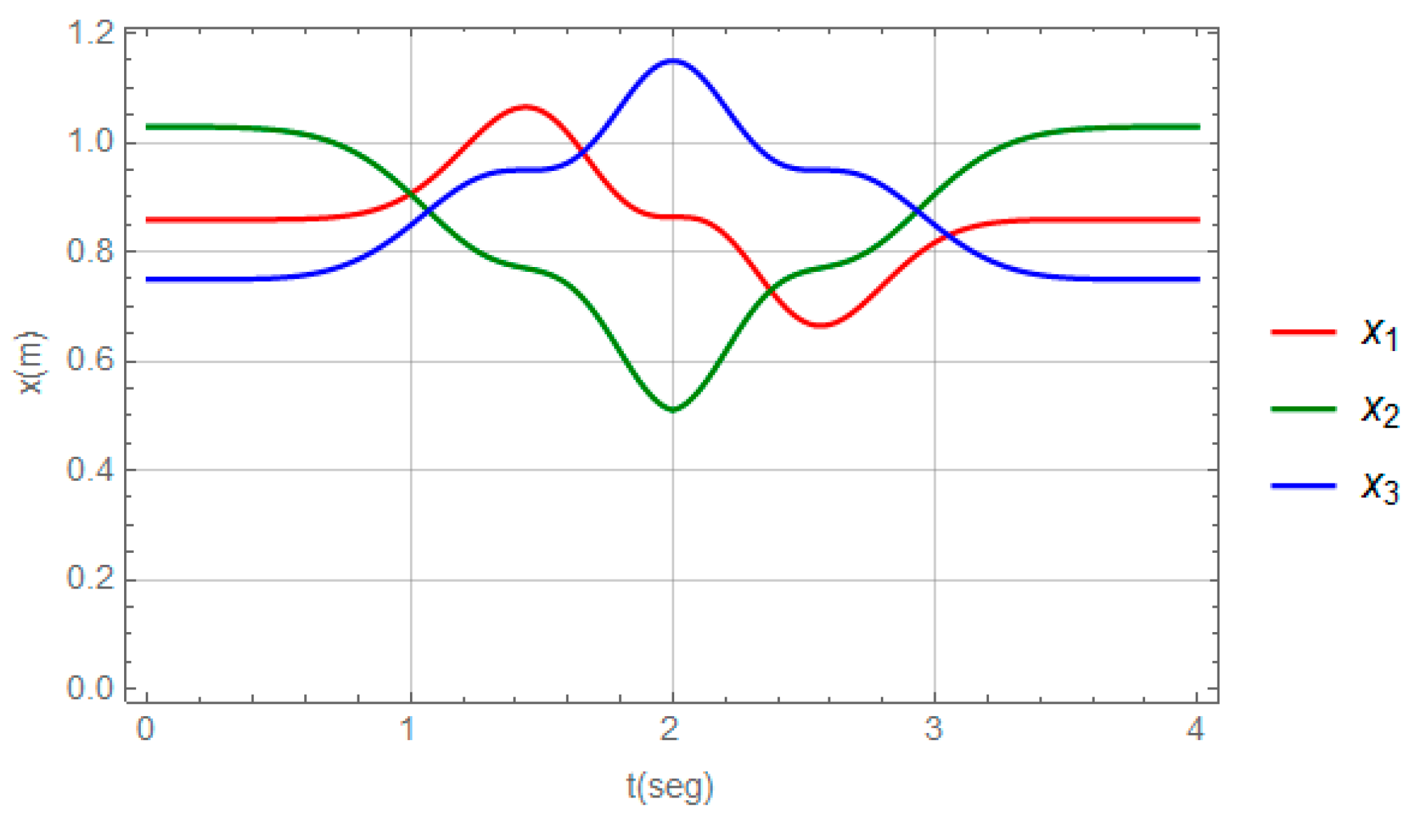
Similarly, the following trajectory is proposed for the PRRS space robot by 0 ≤ t ≤ 4 seconds:
s = 2π(10(t/4)3 − 15(t/4)4 + 6(t/4)5)
xP = 0.75 + 0.2 sin(s)3
yP = 0.75 + 0.2 cos(s)3
zP = 0.75 − 0.2 cos(s)3
The following intervals are defined for platform orientation:
If 0 ≤ t < 2 then ψ = s/6 − π/9
If 2 ≤ t ≤ 4 then ψ = (2π − s)/6 − π/9
θ = 0
φ = 0
The initial configuration of the robot and the graph of the geometric place of the trajectory are shown in Figure 13.
4. Discussion
The methodology presented in this article made it possible to generate the inverse kinematic models of the RRR and PRRS parallel robots in a systematic manner, so that this methodology can be applied to various configurations and types of parallel kinematic chains. The methodological proposal took into consideration the systematization of the quaternion algebra developed by Reyes [25] and applied by Jiménez et al. [24]. The kinematic modeling of the position was a function of the unknown parameters of the quaternions. The binary operations defined by the expressions (1) and the linear transformation described by equation (12), allowed to establish the kinematic modeling in a vectorial way by means of loop equations and platform orientation equations as a multiplication of quaternions representing relative spins in x, y, and z axes. The kinematic modeling developed with the method proposed in this work does not require matrix representations, nor does it take into account in its development the trigonometric functions defined between the parameters of the quaternions given by equation (15), which produces highly nonlinear polynomial equations, which were solved numerically to obtain the parameters or components of the quaternions. On the other hand, the movements of the moving platform of the PRRS robot example were represented by 3 quaternions associated to the 3 DOFs required for its orientation, although a general quaternion can also be used as was the case presented in [28] and [29].
It should be noted that the mathematical models associated with the inverse kinematic problems of each robot were solved by applying the Broyden-Fletcher-Goldfarb-Shanno method [46], which is automated in Mathematica V12 software. With the obtained solutions it was possible to plot the robot movements (see Figure 9 and Figure 17). Two trajectories were taken into account in order to solve the inverse kinematic problem of each robot and thus generate, from a given function, the calculation of the rotations, as well as the linear displacements (for the case of the PRRS robot), related to the RRR type flat robot and the PRRS space robot.
A methodology similar to that of the present work was proposed by Jiménez et al [24]. It is possible to find four important differences between the methodology proposed in this paper and the modeling method developed by Jiménez et al. [24]: the first difference is presented in the study of the movements, since in [24] sequences of rotations were used and the axes of rotation of each rotation were updated in the modeling of the movements of an anthropomorphic RRR robot, while in the modeling of parallel robots developed in this article it was not required to update the axes of rotations, since this process is performed by multiplying quaternions when representing relative spins, resulting in a reduction of operations. The second difference is in the modeling of the robot configurations, since in [24] the initial and final positions of the robot were considered for the construction of the model, while to develop the models of the parallel robots of the present study only the initial position was required, thus simplifying the modeling of the kinematics. The third difference is presented in the configuration of the mathematical models, since in the work developed by Jiménez et al. [24], systems of square equations were formed (same number of equations and unknowns), while the modeling proposed in this article generated systems of non-linear non-square equations, due to the fact that the equation representing the platform orientation is constituted by a multiplication of quaternions that generates four-element vectors and produces extra equations. The advantage of having the orientation equation is that it allows to calculate the angles at all joints. The fourth difference is in the numerical method used, since in [24] having a square system of equations and unknowns, the Newton-Raphson method was used to obtain the numerical solution of the kinematics of a 3 DOF PUMA robot, and in the present study the Broyden-Fletcher-Goldfarb-Shanno quasi-Newton method was applied to solve the rectangular systems of equations of each robot studied.
5. Conclusions
In this article, a methodology to model rigid multibody in the plane and in space using unit quaternions was presented. The methodology was used to model the movements of two parallel robots. The main conclusions are summarized in the following points:
- The methodology proposed in this work and the application of unitary quaternions in the modeling process made it possible to build in a systematic and functional way the mathematical models that define the inverse kinematic problem of a flat RRR-type robot and a PRRS-type space robot.
- The mathematical models generated by the application of the methodology to each robot had the following characteristics: 1) the inverse kinematic problem associated with the RRR robot moving in the plane generated a system of 21 nonlinear equations with 18 unknowns of the polynomial type, and 2) the inverse kinematic problem associated with the PRRS robot moving in space generated a system of 36 nonlinear equations with 33 unknowns of the polynomial type for each kinematic chain.
- To solve the mathematical models generated from the inverse kinematic problem approach in both robots, two linear and angular trajectories were used, and the Broyden-Fletcher-Goldfarb-Shanno numerical method was used to calculate the parameters of the quaternions that define the rotations and displacements of each joint. The BFGS optimization method was used due to the high number of equations and unknowns related to the mathematical models of both robots and the advantage offered by formal calculation packages such as Mathematica V12 that has such method programmed.
- The systematization of unitary quaternions developed by Reyes [25] and applied by Jiménez et al. [24] in the modeling of a PUMA robot, has allowed the construction of kinematic models of parallel robots using the binary operations of addition and multiplication between quaternions. Thus, it was possible to model open and closed kinematic chains in a systematic way, which increases the scope of the theory developed by [25].
The methodology presented in this paper can be extended to the complete kinematic study of parallel robots by incorporating the velocity, acceleration and higher derivative models, and with them, it will be possible to model the dynamics of parallel robots. Likewise, it will be possible to study the direct kinematic problem and mechanism synthesis problems using and improving the methodology.
Author Contributions
Conceptualization and writing, F.C.J.; Analysis and writing, E.J.L.; State of the art, M.A.F.; Proofreading and editing, F.R.P.A.; Research, R.J.P.E..; Supervision J.J.D.V.; Analysis and editing, E.J.L. All authors have read and agreed to the published version of the manuscript.
Funding
This research received no external funding.
Institutional Review Board Statement
Not applicable.
Informed Consent Statement
Not applicable.
Data Availability Statement
Not applicable.
Acknowledgments
The authors of this work thank the National Autonomous University of Mexico, the La Salle Norwest University, the Technological University of Southern Sonora, the Autonomous University of Yucatan, the Autonomous University of the State of Morelos and the Higher Technological Institute of Cajeme for the support and facilities granted for the development of this research. The authors of this work are grateful to their universities and technological institutes for the facilities provided to carry out this research.
Conflicts of Interest
The authors declare no conflict of interest.
Abbreviations
The following abbreviations are used in this manuscript:
| PUMA | Programmable Universal Manipulation Arm |
| DOF | Degree of Freedom |
| BFGS | Broyden-Fletcher-Goldfarb-Shanno |
| RRR | Rotational, Rotational, Rotational |
Appendix A
Appendix A.1
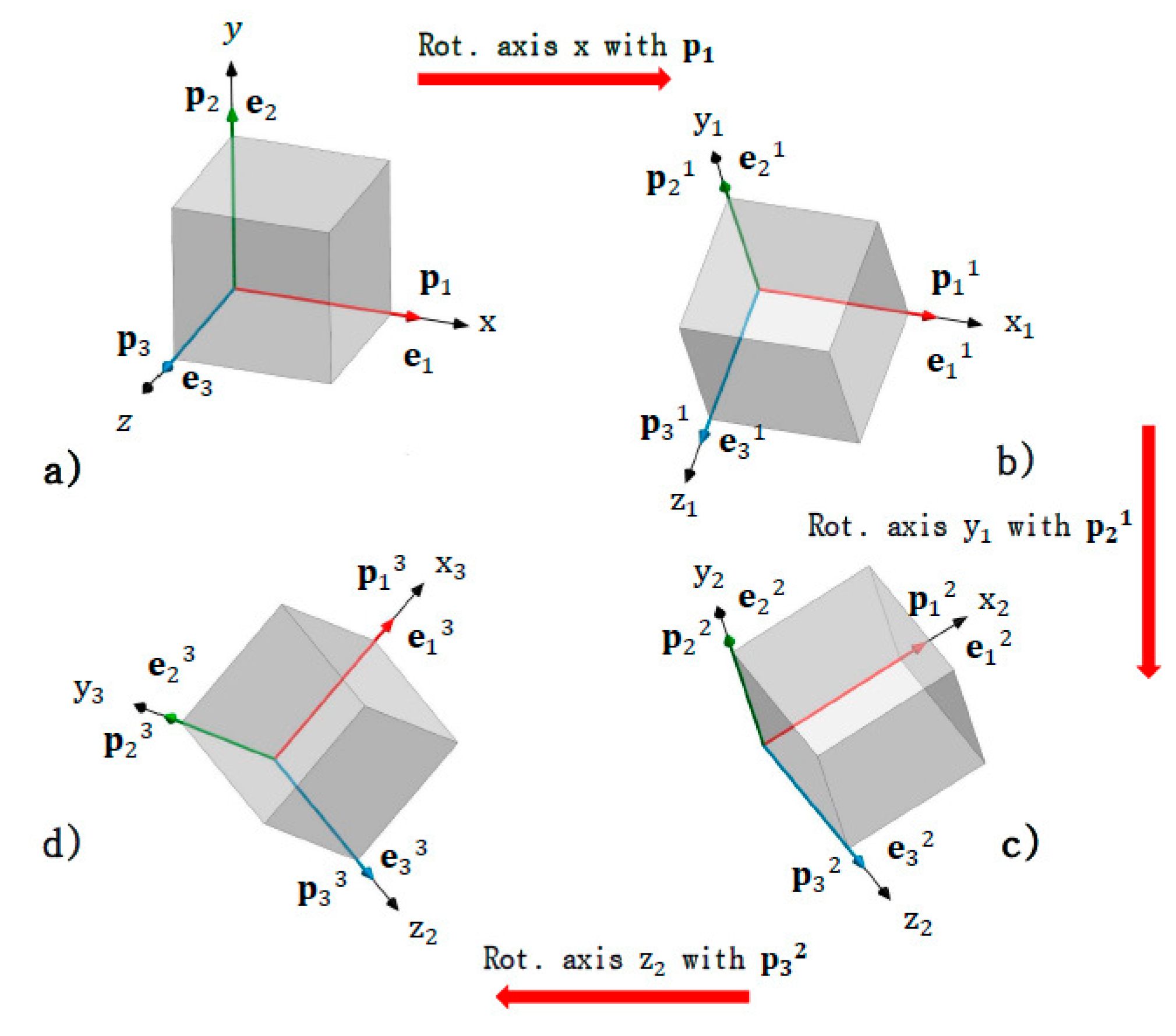
Since the orientation of a rigid body in three-dimensional space is completely defined by three rotations [53], it is possible to define this orientation by the composition of three rotation unitary quaternions. For this purpose, the following considerations are described:
- 1)
- Quaternions p1, p2, p3, are associated to the axes x, y, z, respectively, which will rotate with the body as shown in Figure A.a.
- 2)
- The rotation in the x-axis is produced using the quaternion p1. The ej1 basis elements and the quaternions experience the rotation shown in Figure A.b.
- 3)
- Subsequently, the rotation in the y1 axis is produced using the quaternion p21 (previously rotated). The ej2 basis elements and the quaternions undergo the rotation shown in the Figure. A.c.
- 4)
- Finally, the rotation in the z2 axis is produced using the quaternion p32 (previously rotated). The ej3 basis elements and the quaternions undergo the rotation shown in Figure A.d.
Figure A.
Composition of rotations.
The different orientations of the elements of the bases ej1, ej2, ej3, and the quaternions p21, p32, will be defined analytically by means of the rotation function ρ. Then we have the following proposition:
Proposition. The orientation in space of a local basis ejn attached to a rigid body undergoing three rotations about an inertial basis ej, is expressed as follows:
(A1)
Such that ejn = Tv(ejn) and q = p1*p2*p3, for p1 = (p10, p11, 0, 0), p2 = (p20, 0, p22, 0) and p3 = (p30, 0, 0, p33) quaternions with axis of rotation in x, y, z, respectively.
Demonstration:
Given the quaternions p1 = (p10, p11, 0, 0), p2 = (p20, 0, p22, 0), p3 = (p30, 0, 0, p33), with turning axes on x, y, z, respectively, rotation of the base occurs ej1, and of the quaternions pj1 (Figure A.b), on x-axis by p1. This is:
ej1 = ρ(p1, ej) (A2)
pj1 = ρ(p1, pj) (A3)
Equation (A3) establishes the current position of the rotation quaternions. The rotation of the base ej2 and of the quaternions pj2 (Figure A.c) occurs on the y1 axis through p21, which is represented as follows:
ej2 = ρ(p21, ej1) (A4)
pj2 = ρ(p21, pj1) (A5)
The rotation of the base ej3 and of the quaternions pj3 (Figure A.d) is produced in the z2 axis by p32. This is:
ej3 = ρ(p32, ej2) (A6)
pj3 = ρ(p32, pj2) (A7)
In addition, the following properties are satisfied:
(A8)
(A9)
By substituting equations (A2), (A3) in equation (A4) and using equation (A9), the following equality is obtained:
(A10)
By substituting equation (A3) in equation (A5) and obtaining its conjugate, the following expressions are generated:
(A11)
(A12)
By substituting equations (A10), (A11) and (A12) in the expression (A6) and using the properties (A9), we have:
(A13)
(A14)
(A15)
In addition, the following equality is fulfilled:
(A16)
Substituting equations (A14), (A15) and (A16) in expression (A13) the following expression is generated:
(A17)
Finally, by renaming ej3 by ejn, equation (A17) can be written as follows:
(A18)
where q = p1*p2*p3, which is what was wanted.
References
- Pott, A.; Hiller, M. Kinematic Modeling, Linearization and First-Order Error Analysis, In: Parallel Manipulators, towards New Applications, 1st ed. Ed. Huapeng Wu., Ed. Intechopen, Croatia, 2008; pp. 155-174. [CrossRef]
- Merlet, J.; Gosselin, C. Parallel Mechanisms and Robots. In: Springer Handbook of Robotics, 1st Ed., Siciliano, B.; Khatib, O., Eds. Springer-Verlag, Berlin Heidelberg, 2008, pp. 269-285.
- Himam, S. ; Satish.; G.; Subba, N.V. Relative Kinematic Analysis of Serial and Parallel Manipulators, IOP Conf. Series: Materials Science and Engineering, 2018, 455, 012040. [Google Scholar] [CrossRef]
- Olarra, A.; Axinte, D.; Uriarte, L.; Bueno, R. Machining with the WalkingHex: A walking parallel kinematic machine tool for in situ operations, CIRP Annals, 2017, 66: 361-364. [CrossRef]
- Baptiste, J. On the Improvements of a Cable-Driven Parallel Robot for Achieving Additive Manufacturing for Construction. In: Cable-Driven Parallel Robots. Mechanisms and Machine Science, Gosselin C., Cardou P., Bruckmann T., Pott A. (eds), vol 53. Springer, Cham. 2018, pp 353–363. [CrossRef]
- Li, P.; Shu, T.; Wen, X.; Tian, W. Dynamic Visual Servoing of A 6-RSS Parallel Robot Based on Optical CMM. J Intell Robot Syst 2021, 102, 40. [Google Scholar] [CrossRef]
- Ersoy, O.; Yildirim, M. C.; Ahmad, A.; Yirmibesoglu, O. D.; Koroglu, N.; Bebek, O. Design and Kinematics of a 5-DOF Parallel Robot for Beating Heart Surgery, 2019 IEEE 4th International Conference on Advanced Robotics and Mechatronics (ICARM), Toyonaka, Japan, September, 2019, pp. 274-279. [CrossRef]
- Vaida, C.; Birlescus, I.; Pisla, A.; Ionut, U.; Tarnita, D.; Carbone, J. Systematic Design of a Parallel Robotic System for Lower Limb Rehabilitation, IEEE Access, 2020; 8: 34522-34537. [CrossRef]
- Chang, Z.; Yue, F. Design and Analysis for a Three-Rotational-DOF Flight Simulator of Fighter-Aircraft. Chin. J. Mech. Eng. 2018, 31, 55. [Google Scholar] [CrossRef]
- Wang, S.; Zheng, k.; Chen, Y.; Xu, M.; Wang, D. DOF and kinematics analysis of a 3-UPU parallel mechanism for telescope secondary mirror support, Proc. SPIE 12069, AOPC 2021: Novel Technologies and Instruments for Astronomical Multi-Band Observations, 120690C. Beijing, China, November. 2021. [CrossRef]
- Sholanov, K.S. Kinematics of One-Loop Parallel Manipulators. In: Parallel Manipulators of Robots. Mechanisms and Machine Science, vol 92. Springer, Cham. 2021. [CrossRef]
- Zhang, Y.; Han, H.; Zhang, H.; Xu, Z.; Xiong, Y.; Han, K.; Li, Y. Acceleration analysis of 6-RR-RP-RR parallel manipulator with offset hinges by means of a hybrid method. Mech. Mach. Theory, 2022; 169: 104661. [CrossRef]
- Hamdoun, O.; El Bakkali, L.; Zahra, F. Analysis and Optimum Kinematic Design of a Parallel Robot, Procedia Engineering, 2017; 181: 214-220.
- Yao, S.; Li, H. ; Zeng. Vision-based adaptive control of a 3-RRR parallel positioning system. Sci. China Technol. Sci, 2018; 61: 1253–1264. [CrossRef]
- Baron, N.; Philippides, A.; Rojas, N. A Geometric Method of Singularity Avoidance for Kinematically Redundant Planar Parallel Robots. In: Advances in Robot Kinematics. ARK 2018. Springer Proceedings in Advanced Robotics, Lenarcic, J.; Parenti, V. (eds), vol 8. Springer, Cham. 2019, pp. 187-194. [CrossRef]
- Meng, Q.; Xie, F.; Liu, X.; Takeda, Y. Screw Theory-Based Motion/Force Transmissibility Analysis of High-Speed Parallel Robots with Articulated Platforms. J. Mechanisms Robotics, 2020; 12: 041011. [CrossRef]
- Chai, X.; Wang, M.; Xu, L.; Ye, W. Dynamic Modeling and Analysis of a 2PRU-UPR Parallel Robot Based on Screw Theory, IEEE Access, 2020; 8: 78868-78878. [CrossRef]
- Jiménez, E.; Servín de la Mora, D.; Servín de la Mora, R.; Ochoa, F.; Acosta, M.; Luna, G. Modeling in Two Configurations of a 5R 2-DoF Planar Parallel Mechanism and Solution to the Inverse Kinematic Modeling Using Artificial Neural Network, IEEE Access, 2021; 9: 68583-68594. [CrossRef]
- Thiruvengadam, S.; Tan, J.S. ; Miller., K.A. Generalised Quaternion and Clifford Algebra Based Mathematical Methodology to Effect Multi-stage Reassembling Transformations in Parallel Robots”. Adv. Appl. Clifford Algebras, 2021, 31, 39. [CrossRef]
- Xiang, Y.; Li, Q.; Jiang, X. Dynamic rotational trajectory planning of a cable-driven parallel robot for passing through singular orientations, Mech. Mach. Theory, 2021; 158: 104223. April. 2021. [CrossRef]
- Noppeney, V.; Boaventura, T.; Siqueira, A. Task-space impedance control of a parallel Delta robot using dual quaternions and a neural network. J Braz. Soc. Mech. Sci. Eng. 2021; 43: 440. [CrossRef]
- Liu, K.; Kong, X.; Yu, J. Operation mode analysis of lower-mobility parallel mechanisms based on dual quaternions, Mechanism and Machine Theory, 2019, 152: 103577. [CrossRef]
- Dantam, N. Robust and efficient forward, differential, and inverse kinematics using dual quaternions, Int. J Rob. Res, 2020, 1–19. [CrossRef]
- Jiménez, E.; Servín de la Mora, D.; Reyes, L.; Servín de la Mora, R.; Melendez, J.; López, A. A. Modeling of Inverse Kinematic of 3-DoF Robot, Using Unit Quaternions and Artificial Neural Network”, Robotica; 2021; 39: 1230-1250. [CrossRef]
- Reyes, R. Quaternions: Une Representation Parametrique Systematique Des Rotation Finies. Partie I: Le Cadre Theorique,” In: Rapport de Recherche 1303 INRIA Rocquencourt France. 1990.
- Reyes. R. Quaternions: Une Representation Parametrique Systematique Des Rotation Finies. Partie II: Quelques Application, In: Rapport de Recherche 1454 INRIA Rocquencourt France. 1991.
- Murray, A.; Pierrot, F.; Dauchez, P.; McCarthy, J. A planar quaternion approach to the kinematic synthesis of a parallel manipulator, Robotica, 1997, 15(4): 361-365. [CrossRef]
- Ruggiu, M.; Kong, X. Reconfiguration Analysis of a 3-DOF Parallel Mechanism. Robotics,. 2019, 8: 66.. [CrossRef]
- Liu, Y.; Wu, H.; Liu, H.; Chen, B.; Yao, J.; Wang, Y. Forward kinematics for 6-UPS parallel robot using extra displacement sensor. Journal of Advanced Mechanical Design, Systems, and Manufacturing, 2018, 12(7): 1-11. [CrossRef]
- Birlescu, I.; Husty, M.; Vaida, C.; Gherman, B.; Tucan, P.; Pisla, D. Joint-Space Characterization of a Medical Parallel Robot Based on a Dual Quaternion Representation of SE(3). Mathematics, 2020, 8: 1086. [CrossRef]
- Liu, K.; Kong, X.; Yu, J. Operation mode analysis of lower-mobility parallel mechanisms based on dual quaternions. Mech. Mach. Theory, 2019, 142, 103577. [CrossRef]
- Nigatu, H.; Kim, D. Optimization of 3-DoF Manipulators’ Parasitic Motion with the Instantaneous Restriction Space-Based Analytic Coupling Relation. Appl. Sci. 2021, 11, 4690. [Google Scholar] [CrossRef]
- Kumar, A.; Parhi, D. Dynamic walking of multi-humanoid robots using BFGS Quasi-Newton method aided Artificial potential field approach for uneven terrain, Soft Comput, 2022: 1-16. [CrossRef]
- Xie, S.; Sun, L. , Wang, Z.; Chen, G. A speedup method for solving the inverse kinematics problem of robotic manipulators. Int. J. Adv. Robot. Syst.. 2022: 1-10. [CrossRef]
- Haibo, Q.; Yuefa, F.; Sheng, G. Theory of Degrees of Freedom for Parallel Mechanisms with Three Spherical Joints and Its Applications, Chin. J. Mech. Eng., 2015, 28 (4): 737-746.
- Abdelrahman, S.; Nada, M.; Salem, A.; Hossam, H. Modeling of Nonlinear 3-RRR Planar Parallel Manipulator: Kinematics and Dynamics Experimental Analysis, Int. J. Mech. Mechatron. Eng., 2020, 20 (5): 175-185.
- Zhang, Z.; Wang, L.; Shao, Z. Improving the kinematic performance of a planar 3-RRR parallel manipulator through actuation mode conversion, Mech. Mach. Theory, 2018, 130: 86-108.
- Lianchao, S. , Wei, L. Optimization Design by Genetic Algorithm Controller for Trajectory Control of a 3-RRR Parallel Robot, Algorithms,. 2018, 11, (1): 7.. [CrossRef]
- Sayed, A.S.; Azar, A. T.; Ibrahim, Z.F.; Ibrahim, H.A.; Mohamed, N. A.; Ammar, H.H. Deep Learning Based Kinematic Modeling of 3-RRR Parallel Manipulator. In: Proceedings of the International Conference on Artificial Intelligence and Computer Vision (AICV2020). AICV 2020. Advances in Intelligent Systems and Computing, Hassanien A.E.; Azar A.; Gaber T.; Oliva D.; Tolba F. (eds), vol 1153. Springer, Cham. 2020, pp. 308-321. [CrossRef]
- Al, A.; Aldair, A.A.; Chatwin, C. Control of a 3-RRR Planar Parallel Robot Using Fractional Order PID Controller. Int. J. Autom. Comput. 2020, 17: 822–836. [CrossRef]
- Geng, J.; Arakelian, V. Partial Shaking Force Balancing of 3-RRR Parallel Manipulators by Optimal Acceleration Control of the Total Center of Mass. In: Multibody Dynamics 2019. ECCOMAS 2019. Computational Methods in Applied Sciences, Kecskeméthy A.; Geu, F. (eds), vol 53. Springer, Cham. 2019, pp. 375-382. [CrossRef]
- Gao, Y.; Chen, K.; Gao, H. ; Xiao, P; Wang, L. Small-angle perturbation method for moving platform orientation to avoid singularity of asymmetrical 3-RRR planner parallel manipulator. J Braz. Soc. Mech. Sci. Eng, 2019, 41, 538. [CrossRef]
- Hoang, N. Q.; Vuong, V.D. Inverse Kinematics and Dynamics of a 3RRR Planar Parallel Manipulator in the Presence of Singularities. In: Advances in Asian Mechanism and Machine Science. ASIAN MMS 2021. Mechanisms and Machine Science, Khang, N.V.; Hoang, N.Q.; Ceccarelli M. (eds), vol 113. Springer, Cham. 2021, pp. 228-237. [CrossRef]
- Hall, A.S.; Root, R.R.; Sandgren, E. A Dependable Method for Solving Matrix Loop Equations for The General Three-Dimensional Mechanism, J. Eng. Ind., 1977: 547-550.
- Fischer, I. S.; Paul, R.N. Kinematic Displacement Analysis of a Double-Cardan-Joint Driveline. ASME. J. Mech. Des, 1991, 113(3): 263–271.
- Wolfram Mathematica ® Tutorial Collection Unconstrained Optimization, United States of America, 2008.
- Chen, Z.; Hung, J.C. Application of Quaternion in Robot Control, IFAC Proceedings Volumes, 1987; 20: 259-263. 20. [CrossRef]
- Gouasmi, M.; Ouali, M.; Brahim, F. Robot Kinematics Using Dual Quaternions, Int. J. Robot. Autom., 2021; 1: 13-30.
- Valverde, A.; Tsiotras, P. Spacecraft Robot Kinematics Using Dual Quaternions. Robotics, 2018, 7, 64. [CrossRef]
- Adorno, B. V.; Marques, M. DQ Robotics: A Library for Robot Modeling and Control. IEEE robot. autom. mag., 2020, 28, 102–116. [Google Scholar] [CrossRef]
- Ahmed, A.; Yu, M.; Chen, F. Inverse Kinematic Solution of 6-DOF Robot-Arm Based on Dual Quaternions and Axis Invariant Methods. Arab. J. Sci. Eng., 2022. 47: 15915–15930. [CrossRef]
- Lechuga, L.; Macias, E.; Martínez, G.; Zamora, J.; Bayro, B. Iterative inverse kinematics for robot manipulators using quaternion algebra and conformal geometric algebra. Meccanica, 2022, 57, 1413–1428. [Google Scholar] [CrossRef]
- Suh, C. H.; Radcliffe, C.W. Kinematics and Mechanism Design. John Wiley & Sons, New York, NY, 1978.
- Merlet, J. Les Robots Parallèles. Traité des Nouvelles Technologies - série Robotique. Hermès, Paris, 1990.
- Shigley, J. E. Elementos de Maquinaria. Mecanismos. McGraw Hill, México, 1995.
- Davidon, W.C. Variable metric method for minimization, A.E.C. Research and Development Rept. ANL-5990. 1959. [Google Scholar]
- Mamat, M.; Dauda, M.K.; Mohamed, M.A.; Waziri, M.Y.; Mohamad, F.S.; Abdullah, H. Derivative free Davidon-Fletcher-Powell (DFP) for solving symmetric systems of nonlinear equations, IOP Conf. Ser.: Mater. Sci. Eng. 2018, 332, 012030. [CrossRef]
- Shoham, M.; Li, CJ.; Hacham, Y.; Kreindler, E.; Weill, R. Neural Network Control of Robot Arms. CIRP Annals, 1992, 41(1): 407–410. [CrossRef]
- Acevedo, J.A. Implementation of Quasi-Newton Methods, Thesis, Bachelor's Degree in Applied Mathematics, Faculty of Mathematical-Physical Sciences. Benemérita Universidad Autónoma de Puebla. México, 2019.
Figure 1.
References systems.
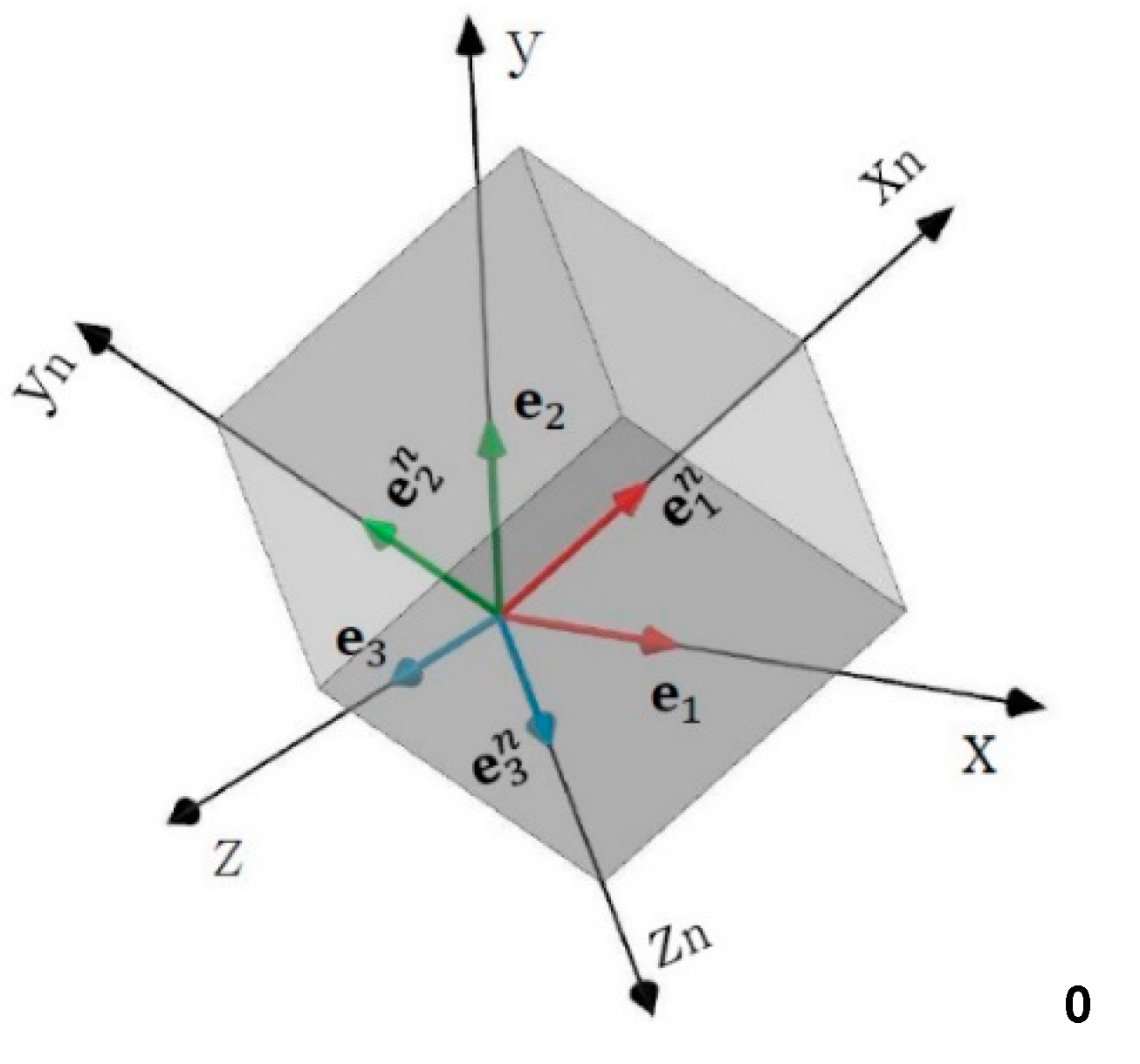
Figure 2.
Articulated links.
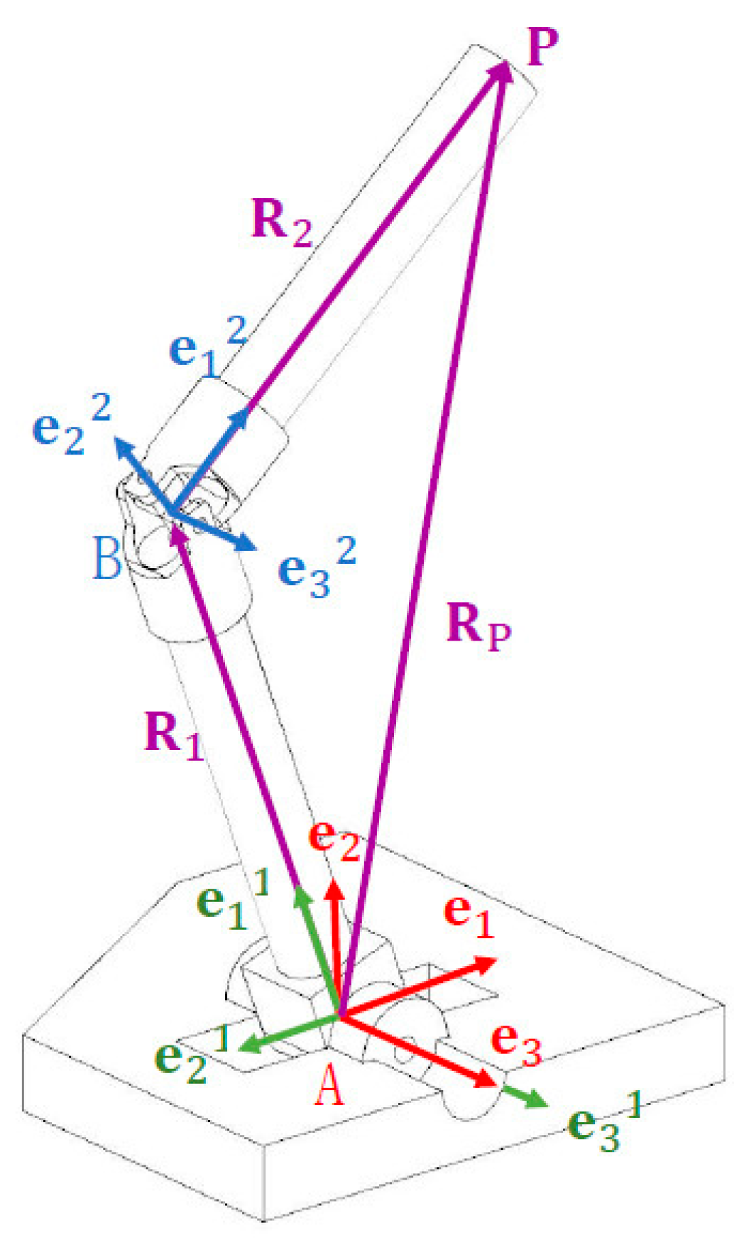
Figure 3.
Configuration of RRR parallel robot.
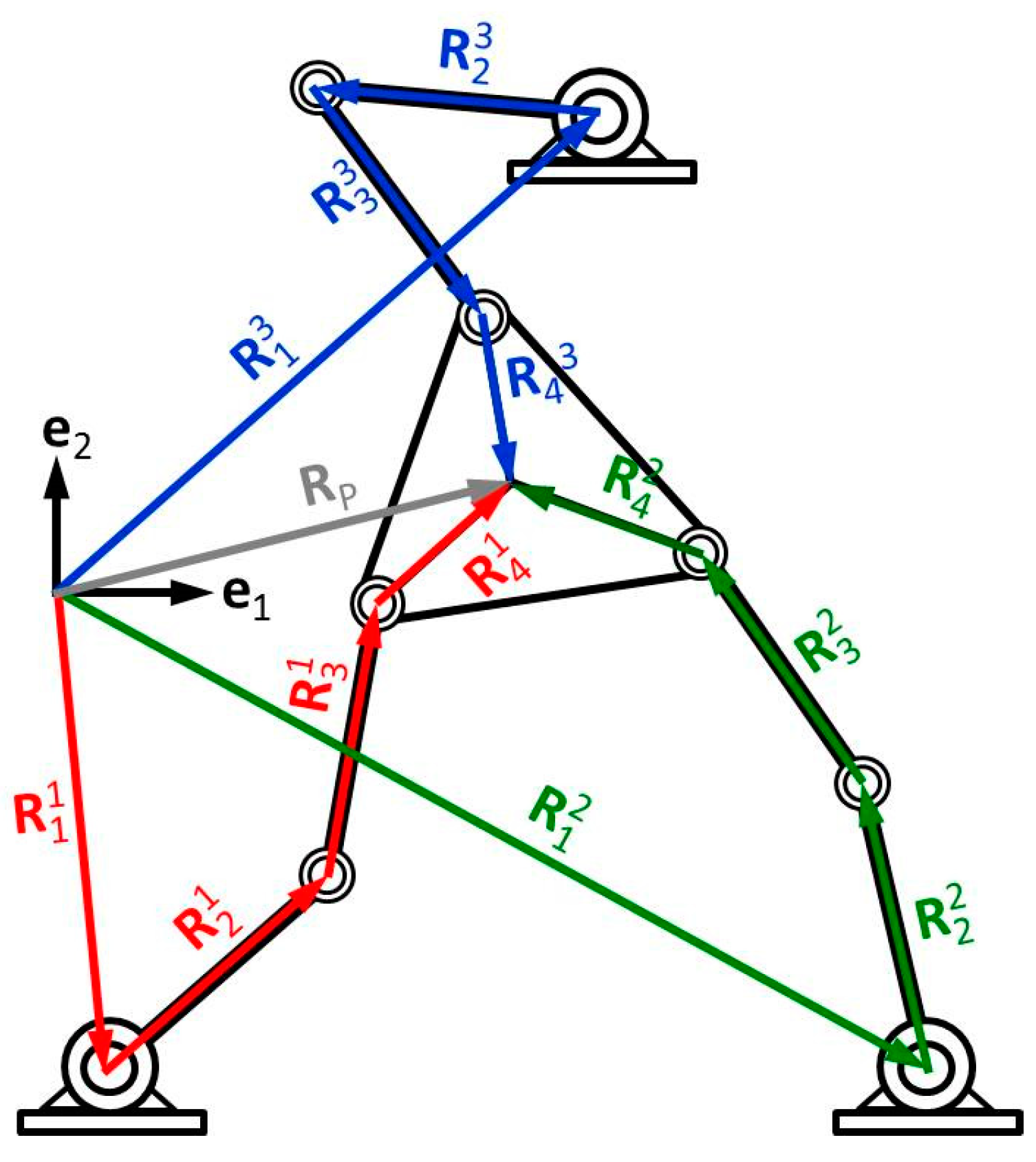
Figure 5.
Angles of the bases.
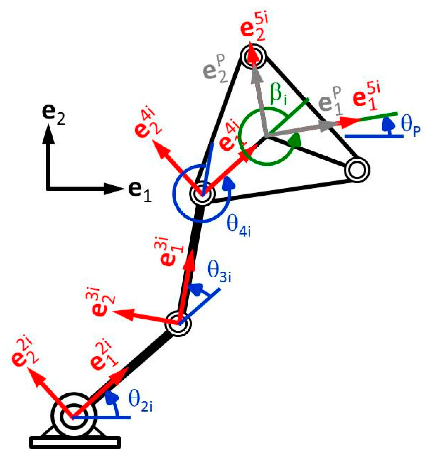
Figure 6.
Configuration of PRRS parallel robot.
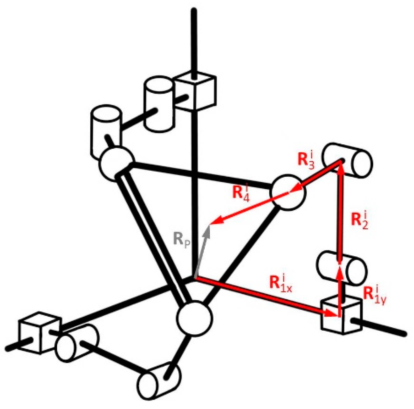
Figure 9.
Mathematica V12 software graphical output of the initial position and orientation of the RRR robot:.
Figure 9.
Mathematica V12 software graphical output of the initial position and orientation of the RRR robot:.
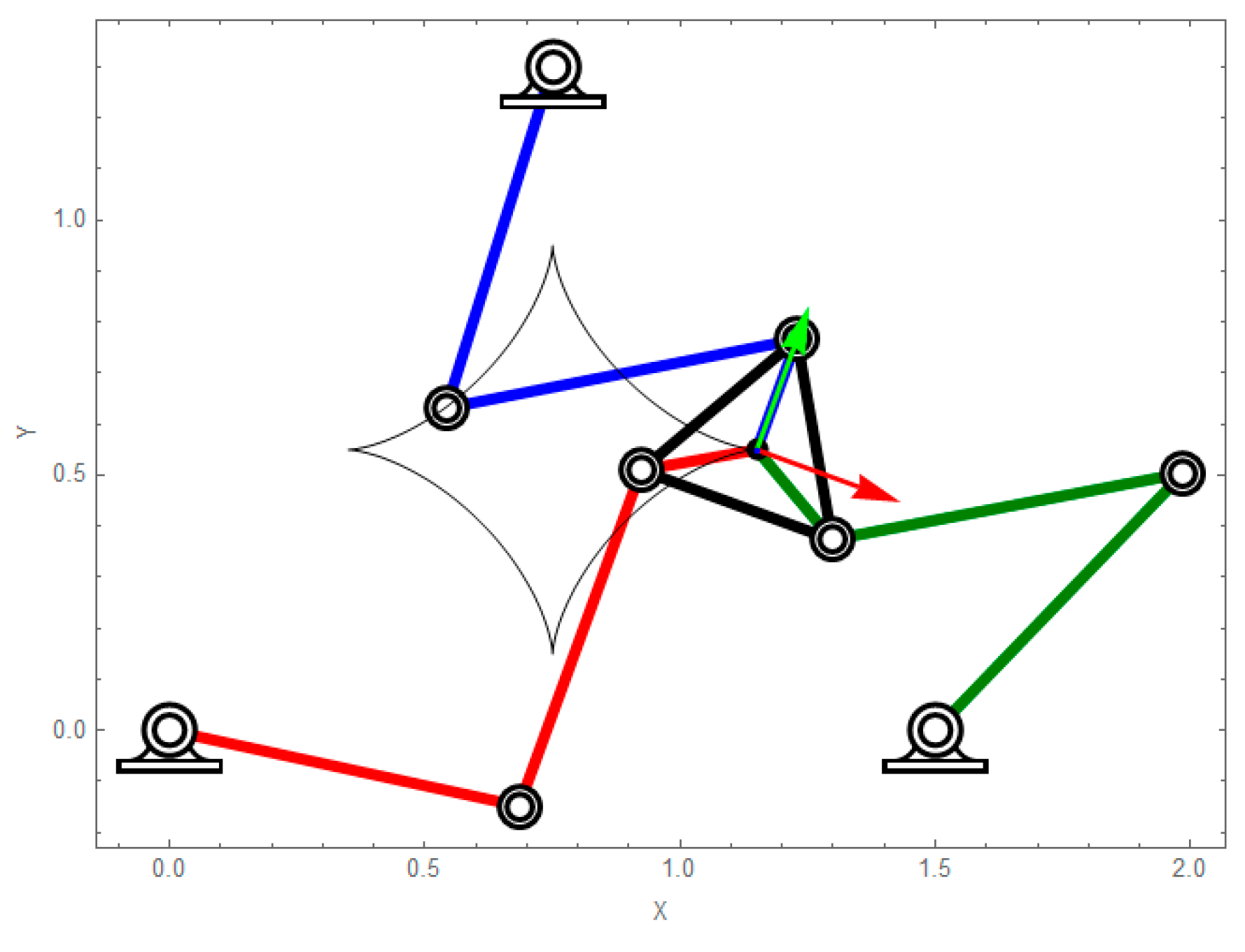
Figure 10.
Angles of chain 1.
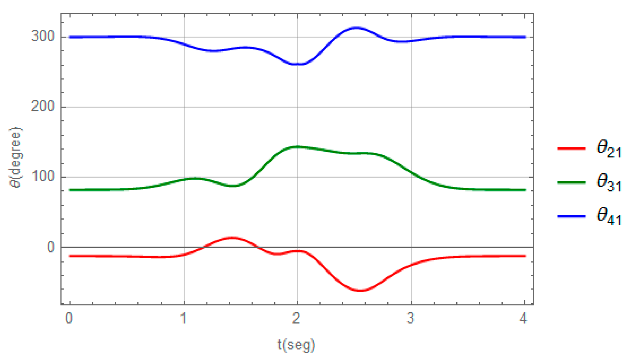
Figure 11.
Angles of chain 2.
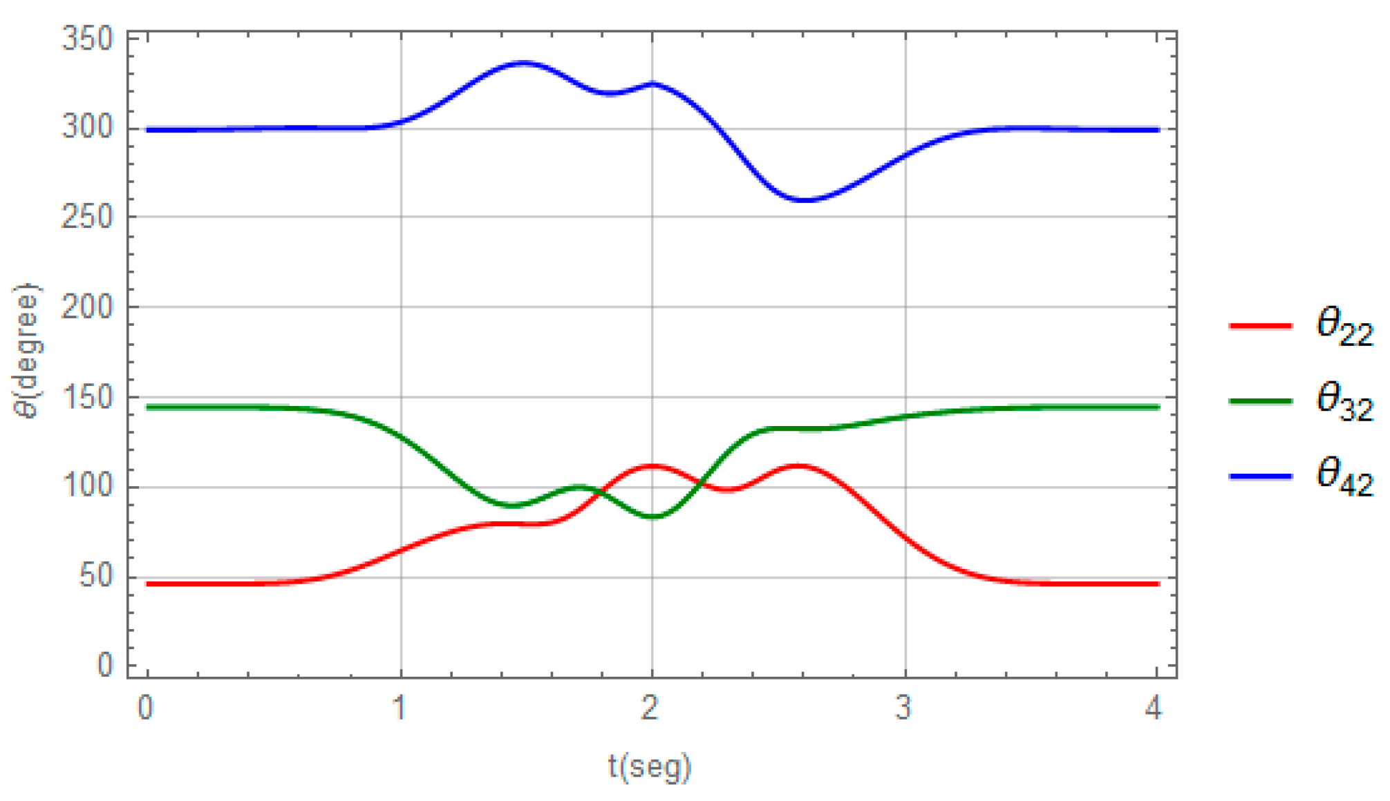
Figure 12.
Angles of chain 3.
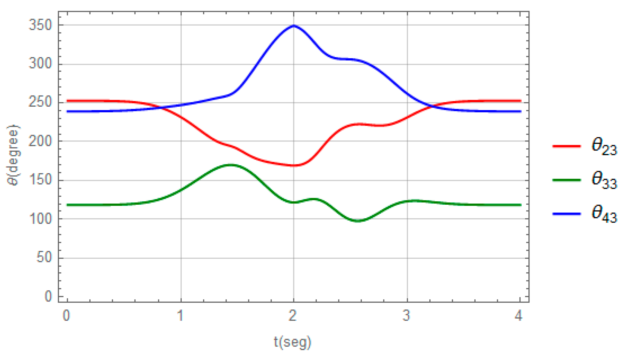
Figure 13.
Mathematica V12 software graphical output of the initial position and orientation of the PRRS robot.
Figure 13.
Mathematica V12 software graphical output of the initial position and orientation of the PRRS robot.
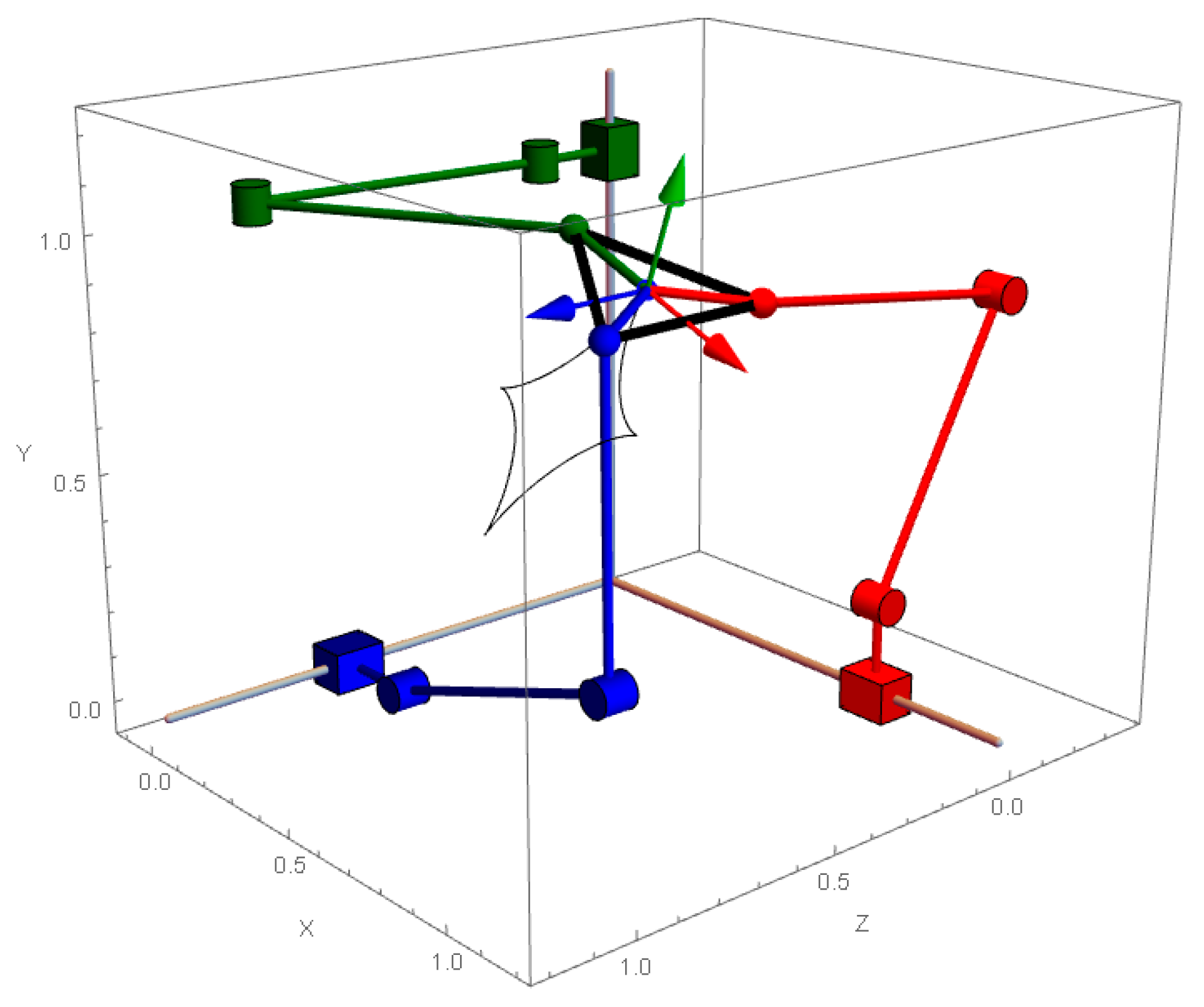
Figure 14.
Angles of chain 1.
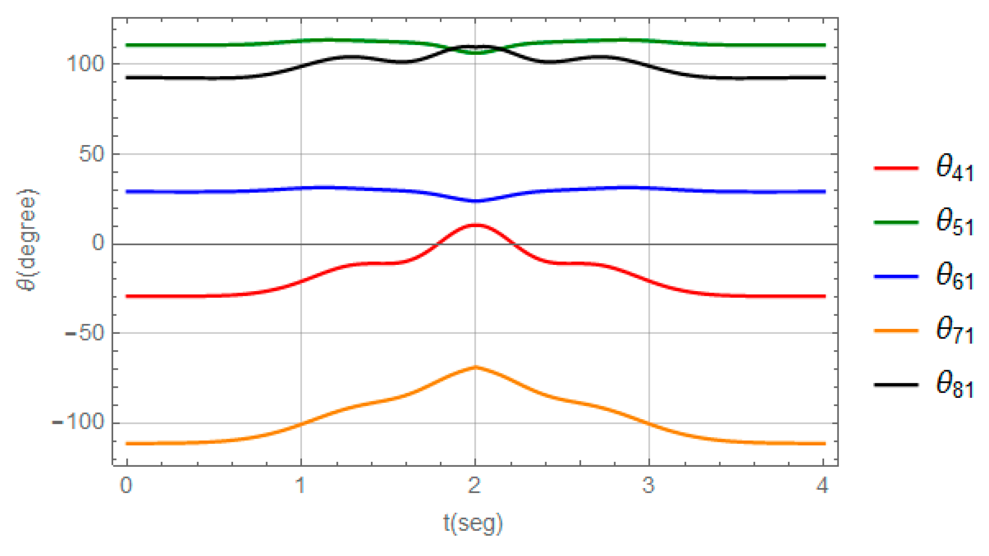
Figure 15.
Angles of chain 2.
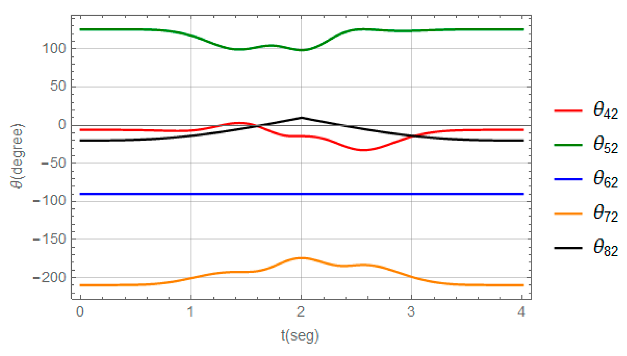
Figure 16.
Angles of chain 3.
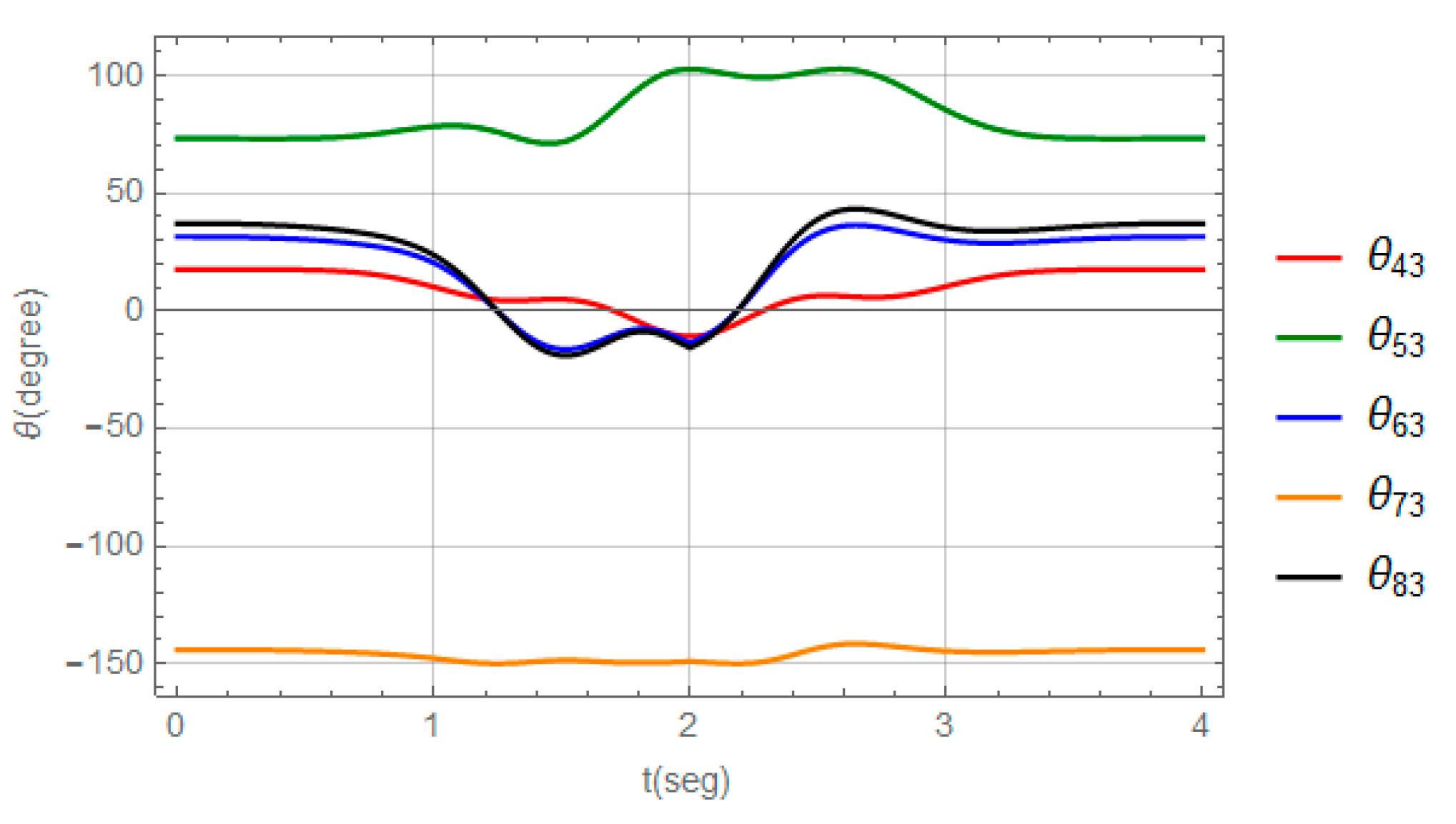
Figure 17.
Displacements of the prismatic joints on the Cartesian axes.
Disclaimer/Publisher’s Note: The statements, opinions and data contained in all publications are solely those of the individual author(s) and contributor(s) and not of MDPI and/or the editor(s). MDPI and/or the editor(s) disclaim responsibility for any injury to people or property resulting from any ideas, methods, instructions or products referred to in the content. |
© 2025 by the authors. Licensee MDPI, Basel, Switzerland. This article is an open access article distributed under the terms and conditions of the Creative Commons Attribution (CC BY) license (http://creativecommons.org/licenses/by/4.0/).
Copyright: This open access article is published under a Creative Commons CC BY 4.0 license, which permit the free download, distribution, and reuse, provided that the author and preprint are cited in any reuse.


