
Submitted:
14 February 2025
Posted:
17 February 2025
You are already at the latest version
Abstract
Rotation motion in a three-dimensional physical world refers to an angular displacement of an object around a specific axis in $\mathbb{R}^3$. It is typically formulated as a non-linear and non-convex motion due to the nonlinearity and nonconvexity of $\mathbb{SO}(3)$. However, this paper proposes a new perspective that the 3D rotation motion can be expressed by a linear system without dropping any constraints and increasing any singularities. Moreover, two frequent cases, i.e., $\angle\left(\mathbf{R}\boldsymbol{x},\boldsymbol{y}\right)=0$ and $\angle\left(\mathbf{R}\boldsymbol{x},\boldsymbol{y}\right)=\frac{\pi}{2}$, in computer vision and robotics that can be expressed linearly are deeply discussed in this paper.
Keywords:
Rotation Motion
; SO(3)
; Clifford Torus
; Unit Quaternion Sphere
1. Introduction
Rotational motion [1] in the three-dimensional physical world is regarding to the circular movement of an object around a fixed axis [2]. It is a basic concept and commonly used in physics, computer graphics, computer vision, robotics, aerospace, and other scientific fields [3,4,5,6]. More specifically, in many practical applications, rotational motion is not only an important way of constructing the motion of the target system [7,8,9] but also an important state parameter to be estimated [10,11,12]. However, rotation motion is typically formulated as a non-linear and non-convex process [11,12,13]. It not only makes some linear algorithms, such as Kalman filter [14,15], impossible to directly apply [16], but also makes solving the related problem more sophisticated and difficult [13,17].
In this paper, a new perspective is proposed that the rotation motion can be linearized without dropping any constraints and increasing any singularities. It is particularly worth pointing out that there are no special and advanced techniques, such as Lie groups and Lie algebras [18,19], for the methods used in this paper. Only some basic knowledge of linear algebra [20,21,22] is required to understand the ideas presented in this paper.
The structure of this paper is as follows: it first reviews rotational motion in the second section, then presents the linearized expression for rotation in the third section. The fourth and fifth sections discuss two special cases,i.e., and , providing in-depth analysis.
2. Rotation Motion
Mathematically, given a point , if it is rotated about a fixed unit vector through the origin and the rotated angle is , then the rotation motion can be formulated by multiplication of a matrix and a vector,
where is the rotated point by and is a rotation matrix. There are some properties regarding the rotation motion [23],
-
Shape and Size: Rotation does not alter the shape or size of the object. More Specifically,
- . It means the length of the point will not be changed by rotation motion. Without loss of generality, the rotation motion in this paper is studied with unit norm vectors, i.e., on the unit sphere surface, which represents a unit direction vector in the 3D physical world.
- where are any two unit vectors. It means the angle (structure) of the object is unchanged.
- Axis of Rotation: Rotational motion occurs around a fixed axis. Given a vector , if , it means the after the rotation , the vector direction remains unchanged, and the vector must be parallel to the rotation axis , which is from Euler’s rotation theorem and screw theory [24,25,26,27]. In addition,where is the 3 × 3 identity matrix. Algebraically, Eq.(2) means the rotation axis direction lies in the null space of . Alternatively, let , then the rotation axis direction is an eigenvector of corresponding to the eigenvalue .
At first glance, the rotation motion is a linear process, which might be misled by the matrix representation Eq.(1). Unfortunately, is not a regular matrix in . A rotation only has three degrees of freedom, since it can be determined by a rotation axis and a rotation angle . Formally, , and a rotation can be represented by a matrix and non-linear constraints,
According to the famous Rodrigues’ rotation formula [28,29], given the rotation axis and rotation angle , the matrix can be constructed by
Moreover, a rotation matrix can be represented by a quaternion vector with unit length [30,31], such that . Specifically,
It is worth noting that many different forms of parameter representation can represent the same rotation, and each form of representation has its appropriate application scenario [32,33,34,35]. For example, since a rotation can be determined by a fixed rotation axis and a rotation angle , then the rotation can be represented by axis–angle representation [36], which geometrically is a point in a 3D ball of radius [29] and has been widely used in pose estimation problems [29,37,38]. Nonetheless, throughout most of this paper, quaternions are used to represent rotations [30,31] and thus to illustrate the proposed linearization theory.

3. Linear Expressions for Rotation Motion
Given and a rotation , the rotation motion can be formulated as
where is rotated by . This formulation is actually a special case of the general rotational motion. Generally, given and whose quaternion expression is , consider an arbitrary angle , there is
Here is constructed by and [30,40]. Specifically,
When , Eq.(7) degenerates back to Eq.(6).
It is worth noting that there are two facts concerning ,

For the first point, it is understandable. For the second point, observe , where is a rotation whose rotation axis is and rotation angle is ; is an arbitrary angle. It means if satisfy , then there are an infinite number of rotations that also satisfy the given rotation motion. Therefore, given a rotation constraint , all rotations that satisfy the given rotation motion should be in some special regions in .
By conducting eigendecomposition of the real symmetric matrix [22,41], where and is an orthogonal matrix . Observe
Therefore, the eigenvalue matrix of is
Accordingly, .
Let , then . Observe
Therefore, it can be formulated
As a consequence, the possible rotation can be reformulated linearly
where . This result clearly shows that the rotational motion can be expressed in linear forms.
Geometrically, if , then all possible rotation that satisfy the constraint will be in a two-dimensional torus in . For better understanding, some special cases can be visualized, i.e., via stereographic projection [42,43], as in Figure 1.
4. Special Case I: Great Circle in
If , which means , it is one of the most common cases in practical applications [33,37]. Then according to Eq. (15) all rotations that satisfy should be in
where and are the basis vectors in , and they depend on , i.e., and . Geometrically speaking, is a unit vector in , which is a linear combination of the two vectors and . In addition, , which means is on the surface of the unit quaternion sphere. Therefore, the region where all possible rotations satisfy a specific rotation motion is a great circle in [44].
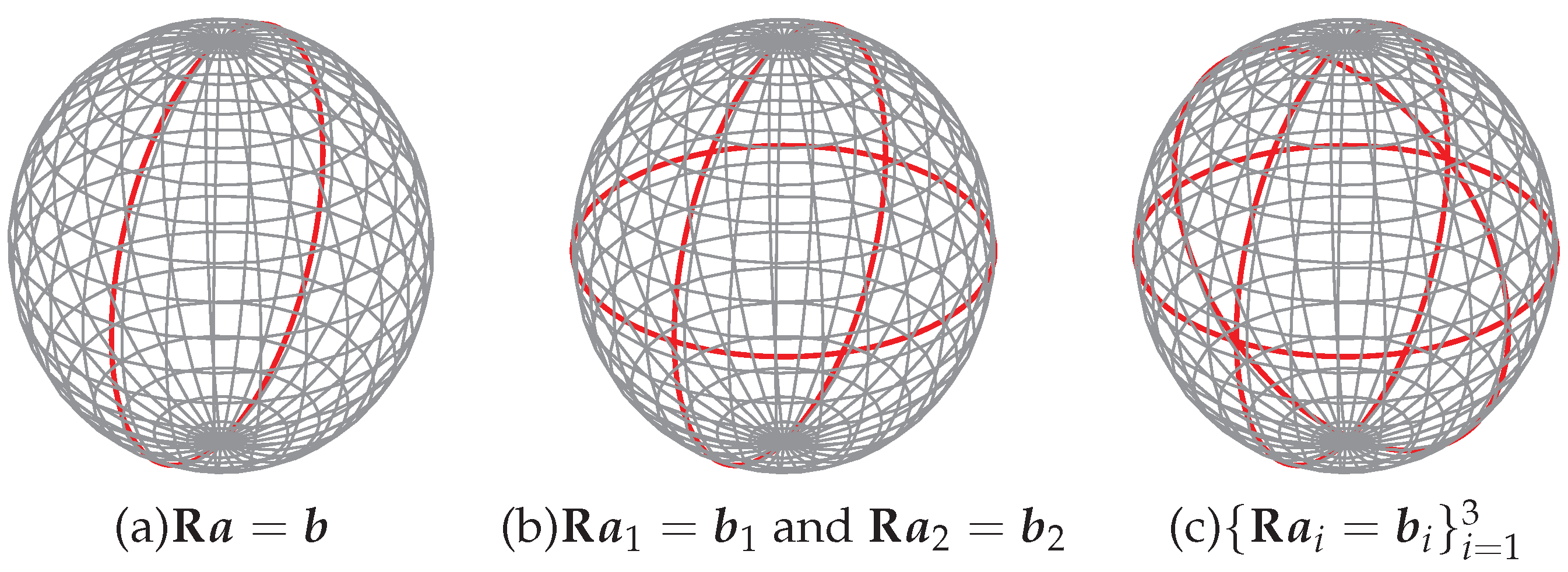
Figure 2.
The illustration of great circles in ; for better visualization, they is imitatively drawn in . (a) Given , all possible solution of the to-be-solved rotation will be in a circle-shape region on (b) Given two rotation motion, there are two circles on the surface, and the intersections of the circles are the solutions that meet both rotation motions. Note that the intersections are symmetrical on the surface, and they are corresponding to the same rotation matrix. (c) Given more rotation motions, there are more circles. The intersections of the circles should be the rotation solution meet all given rotation motions.
In order to determine a unique rotation, two independent constraints are required. Specifically, given two pair of inputs and , two circles can be calculated according to Eq.(17), which is however not easy.
In fact, it does not need to be that complicated. Since , there will be
Consequently, given , there will be , where and are constructed by and . Given and , there will be
Similarly, given N inputs, , there will be
Up until this point, the rotation motion can be surprisingly linearly solved.
4.1. Eigenvector of
It is worth noting that the linear expression of rotation motion is closely related to . Due to , there will be
It is easy to confirm [49,50],
Therefore, any row of can be the eigenvector of with eigenvalue . Similarly, any row of can be the eigenvector of with eigenvalue 1.
Accordingly, there will be
- any row of is a linear combination of and .
- any row of is a linear combination of and .
Consequently, ; and are not necessarily orthogonal matrices. Nonetheless, there is still , more specifically,
5. Special Case II: Clifford Torus in
In the previous description, we provide a general derivation for the connection between rotation constraint, i.e., and Clifford torus. Here we show an alternative way to obtain a Clifford torus from rotation constraint.
Given a rotation constraint , the possible rotation can be (see Figure 3)
where , and ; is a rotation that rotates to ; and are rotations around directions and , respectively. The rotation motion can be as follows,
To use quaternion to represent rotation [30]
The formula for the multiplication of two quaternions is [30]
Define , then
In addition, let and ,
Then,
Therefore,
where
It is easy to verify
Geometrically, Eq. (39) describes a Clifford torus [51] in .
5.1. Intersections of Two Different Clifford Tori
Given two rotation constraints and , the possible rotation can be considered in the intersections of two Clifford tori (see Figure 4). Here, a solution to solve the intersection line is presented. Specifically,
where and is an arbitrary vector and satisfies ; is a specific arbitrary rotation that can rotate to ; and .
According to Rodrigues’ rotation formula [3], we have
Therefore,
Clearly, Eq.(48) shows a one-dimensional curve constructed by and (see Figure 5).
Specifically, given a , would be computed by Eq. (48). Intuitively, one should solve the following equation
where , and . According to the tangent half-angle formula, when ,
Accordingly, can be computed and rotation can be computed as well. Formally,
5.2. Intersections of Three Different Clifford Tori
Given three rotation constraints , and , the possible rotation can be considered in the intersections of three Clifford tori. Note that it belongs to the famous E3Q3 problem [52], and there are many solutions have been proposed to solve it [53,54,55,56,57]. Here this paper provides a more straight linear way. Specifically,
Therefore,
There are two unknown variables and for two constraints, and the intersections can be computed. According to tangent half-angle formula (a.k.a. Weierstrass substitution formulas),
Let , and , and when , ,
The system of equations can be reformulated as
where and , Specifically,
and * is to calculate the matrix item by item. Geometrically, if only considering real solutions, it describes the intersections of two cures computed by observations in plane (see Figure 6).
Algebraically, it is a polynomial system containing two equations in two variables, which can be generally solved by resultant-based method [58,59]. We donate
Both sides of the equations are multiplied by x,
By stacking equations,
To solve y, it is to solve . This determinant is also known as a hidden-variable resultant in computer vision filed [60,61], and it is an univariate polynomial with degree 8 of the hidden variable y.
In fact, the problem is not very complex, one can directly calculate the explicit expression of each term for the resultant-based method using symbolic math. Practically, one can obtain explicit coefficients by the function resultant in Matlab 1 or the function sympy.polys.polytools.resultant in SymPy2, and this paper will not list all details to avoid long-and-tedious expressions for readability. Nonetheless, the solution of y can be directly computed by solving roots of a univariate polynomial [62,63]. After solving y, it is easy to calculate x.
5.2.1. Linear Solution to Solve Intersections of Three Different Clifford Tori
Alternatively, Eq. (64) can be rewritten as a quadratic eigenvalue problem, i.e., [60,61,64].
where , and . Specifically,
Notably, there is no x and y in , and . Accordingly, it is easy to solve the system of polynomial equations by linear way [64].
Conflicts of Interest
The author declares no conflicts of interest.
References
- Waldron, K.J.; Schmiedeler, J. Kinematics. In Springer handbook of robotics; 2016; pp. 11–36. [Google Scholar]
- Ivanov, A. Theoretical matrix study of rigid body general motion. Greener Journal of Physics and Natural Sciences 2017, 3, 009–020. [Google Scholar] [CrossRef]
- Hartley, R.; Zisserman, A. Multiple view geometry in computer vision; Cambridge university press, 2003. [Google Scholar]
- Yehia, H.M. Rigid Body Dynamics. In Advances in Mechanics and Mathematics. Birkhäuser Cham; 2022.
- Teisseyre, R. Tutorial on new developments in the physics of rotational motions. Bulletin of the Seismological Society of America 2009, 99, 1028–1039. [Google Scholar] [CrossRef]
- Kisantal, M.; Sharma, S.; Park, T.H.; Izzo, D.; Märtens, M.; D’Amico, S. Satellite pose estimation challenge: Dataset, competition design, and results. IEEE Transactions on Aerospace and Electronic Systems 2020, 56, 4083–4098. [Google Scholar] [CrossRef]
- Gul, F.; Rahiman, W.; Nazli Alhady, S.S. A comprehensive study for robot navigation techniques. Cogent Engineering 2019, 6, 1632046. [Google Scholar] [CrossRef]
- Yefymenko, N.; Kudermetov, R. Quaternion models of a rigid body rotation motion and their application for spacecraft attitude control. Acta Astronautica 2022, 194, 76–82. [Google Scholar] [CrossRef]
- Rizzi, G.; Ruggiero, M.L. Relativity in rotating frames: relativistic physics in rotating reference frames, Springer, 2004.
- Bustos, A.P.; Chin, T.J. Guaranteed Outlier Removal for Point Cloud Registration with Correspondences. IEEE transactions on pattern analysis and machine intelligence 2018, 40, 2868–2882. [Google Scholar] [CrossRef]
- Eriksson, A.; Olsson, C.; Kahl, F.; Chin, T.J. Rotation Averaging with the Chordal Distance: Global Minimizers and Strong Duality. IEEE Transactions on Pattern Analysis & Machine Intelligence 2021, 43, 256–268. [Google Scholar]
- Crassidis, J.L.; Markley, F.L.; Cheng, Y. Survey of nonlinear attitude estimation methods. Journal of guidance, control, and dynamics 2007, 30, 12–28. [Google Scholar] [CrossRef]
- Carlone, L.; et al. Estimation Contracts for Outlier-Robust Geometric Perception. Foundations and Trends® in Robotics 2023, 11, 90–224. [Google Scholar] [CrossRef]
- Mathavaraj, S.; Butcher, E.A. SE (3)-constrained extended Kalman filtering for rigid body pose estimation. IEEE Transactions on Aerospace and Electronic Systems 2021, 58, 2482–2492. [Google Scholar] [CrossRef]
- Welch, G.F. Kalman filter. Computer Vision: A Reference Guide, 2020; 1–3. [Google Scholar]
- Trawny, N.; Roumeliotis, S.I. Indirect Kalman filter for 3D attitude estimation. University of Minnesota, Dept. of Comp. Sci. & Eng., Tech. Rep 2005, 2, 2005. [Google Scholar]
- Chin, T.J.; Suter, D. The maximum consensus problem: recent algorithmic advances; Springer Nature, 2022. [Google Scholar]
- Etingof, P. Lie groups and Lie algebras. arXiv, 2022; arXiv:2201.09397 2022. [Google Scholar]
- Dehmamy, N.; Walters, R.; Liu, Y.; Wang, D.; Yu, R. Automatic symmetry discovery with lie algebra convolutional network. Advances in Neural Information Processing Systems 2021, 34, 2503–2515. [Google Scholar]
- Gill, P.E.; Murray, W.; Wright, M.H. Numerical linear algebra and optimization, SIAM,, 2021.
- Farin, G.; Hansford, D. Practical linear algebra: a geometry toolbox; Chapman and Hall/CRC, 2021.
- Horn, R.A.; Johnson, C.R. Matrix analysis; Cambridge university press, 2012.
- Taubin, G. 3D Rotations. IEEE Computer Graphics and Applications 2011, 31, 84–89. [Google Scholar] [CrossRef]
- Ball, R.S. The theory of screws: A study in the dynamics of a rigid body. Mathematische Annalen 1876, 9, 541–553. [Google Scholar] [CrossRef]
- Palais, B.; Palais, R. Euler’s fixed point theorem: The axis of a rotation. Journal of fixed point theory and applications 2007, 2, 215–220. [Google Scholar] [CrossRef]
- Kumar, V. The Theorems of Euler and Chasles. University of Pennsylvania School of Engineering and Applied Science, I-Net, USA 2000.
- Joseph, T. An alternative proof of Euler’s rotation theorem. The Mathematical Intelligencer 2020, 42, 44–49. [Google Scholar] [CrossRef]
- Fraiture, L. A history of the description of the three-dimensional finite rotation. The Journal of the Astronautical Sciences 2009, 57, 207–232. [Google Scholar] [CrossRef]
- Hartley, R.I.; Kahl, F. Global optimization through rotation space search. International Journal of Computer Vision 2009, 82, 64–79. [Google Scholar] [CrossRef]
- Jia, Y.B. Quaternions and rotations. Com S 2008, 477, 15. [Google Scholar]
- Spring, K.W. Euler parameters and the use of quaternion algebra in the manipulation of finite rotations: a review. Mechanism and machine theory 1986, 21, 365–373. [Google Scholar] [CrossRef]
- Bauchau, O.; Bauchau, O. Parameterization of rotation. Flexible Multibody Dynamics, 2011; 511–542. [Google Scholar]
- Hartley, R.; Trumpf, J.; Dai, Y.; Li, H. Rotation averaging. International journal of computer vision 2013, 103, 267–305. [Google Scholar] [CrossRef]
- Kim, S.; Kim, M. Rotation representations and their conversions. IEEE Access 2023, 11, 6682–6699. [Google Scholar] [CrossRef]
- Shuster, M.D. A survey of attitude representation. Journal of The Astronautical Sciences 1993, 41, 439–517. [Google Scholar]
- Liu, Y. Globally Optimal Solutions for Unit-Norm Constrained Computer Vision Problems. Ph.D. Thesis, Technische Universität München, 2022. [Google Scholar]
- Liu, Y.; Dong, Y.; Song, Z.; Wang, M. 2D-3D Point Set Registration Based on Global Rotation Search. IEEE Transactions on Image Processing 2019, 28, 2599–2613. [Google Scholar] [CrossRef]
- Yang, J.; Li, H.; Campbell, D.; Jia, Y. Go-ICP: A globally optimal solution to 3D ICP point-set registration. IEEE transactions on pattern analysis and machine intelligence 2015, 38, 2241–2254. [Google Scholar] [CrossRef]
- Altmann, S.L. Rotations, quaternions, and double groups, Courier Corporation, 2005.
- HORN, B.P. Closed-form solution of absolute orientation using unit quaternions. Journal of the Optical Society of America. A, Optics and image science 1987, 4, 629–642. [Google Scholar] [CrossRef]
- Peng, L.; Tsakiris, M.C.; Vidal, R. Arcs: Accurate rotation and correspondence search. In Proceedings of the Proceedings of the IEEE/CVF Conference on Computer Vision and Pattern Recognition; 2022; pp. 11153–11163. [Google Scholar]
- McClintock, P. Relating plane transformations with stereographic projection. Ph.D. Thesis, 2022. [Google Scholar]
- Wilkins, D.R. Möbius transformations and stereographic projection, 2017.
- Gluck, H.; Warner, F.W. Great circle fibrations of the three-sphere. Duke Mathematical Journal 1983, 50, 107–132. [Google Scholar] [CrossRef]
- Bayro-Corrochano, E. A survey on quaternion algebra and geometric algebra applications in engineering and computer science 1995–2020. IEEE Access 2021, 9, 104326–104355. [Google Scholar] [CrossRef]
- Nastro, V.; Tancredi, U. Great circle navigation with vectorial methods. The Journal of navigation 2010, 63, 557–563. [Google Scholar] [CrossRef]
- Cheng, Q.M.; Ishikawa, S. A characterization of the Clifford torus. Proceedings of the American Mathematical Society 1999, 127, 819–828. [Google Scholar] [CrossRef]
- Yu, T.; Chen, J. Uniqueness of Clifford torus with prescribed isoperimetric ratio. Proceedings of the American Mathematical Society 2022, 150, 1749–1765. [Google Scholar] [CrossRef]
- Srivatsan, R.A.; Rosen, G.T.; Mohamed, D.F.N.; Choset, H. Estimating SE (3) elements using a dual quaternion based linear Kalman filter. In Proceedings of the Robotics: Science and systems; 2016. [Google Scholar]
- Arun Srivatsan, R.; Zevallos, N.; Vagdargi, P.; Choset, H. Registration with a small number of sparse measurements. The International Journal of Robotics Research 2019, 38, 1403–1419. [Google Scholar] [CrossRef]
- Andersson, O.; Bengtsson, I. Clifford tori and unbiased vectors. Reports on mathematical physics 2017, 79, 33–51. [Google Scholar] [CrossRef]
- Kukelova, Z.; Heller, J.; Fitzgibbon, A. Efficient intersection of three quadrics and applications in computer vision. In Proceedings of the Proceedings of the IEEE Conference on Computer Vision and Pattern Recognition; 2016; pp. 1799–1808. [Google Scholar]
- Xu, C.; Zhang, L.; Cheng, L.; Koch, R. Pose estimation from line correspondences: A complete analysis and a series of solutions. IEEE transactions on pattern analysis and machine intelligence 2016, 39, 1209–1222. [Google Scholar] [CrossRef] [PubMed]
- Yu, Q.; Xu, G.; Cheng, Y. An efficient and globally optimal method for camera pose estimation using line features. Machine Vision and Applications 2020, 31, 1–11. [Google Scholar] [CrossRef]
- Wang, P.; Xu, G.; Cheng, Y.; Yu, Q. Camera pose estimation from lines: a fast, robust and general method. Machine Vision and Applications 2019, 30, 603–614. [Google Scholar] [CrossRef]
- Chan, K. A simple mathematical approach for determining intersection of quadratic surfaces. In Multiscale optimization methods and applications; Springer, 2006; pp. 271–298. [Google Scholar]
- Sarraga, R.F. Algebraic methods for intersections of quadric surfaces in GMSOLID. Computer Vision, Graphics, and Image Processing 1983, 22, 222–238. [Google Scholar] [CrossRef]
- Sturmfels, B. Introduction to resultants. In Proceedings of the Proceedings of Symposia in Applied Mathematics. American Mathematical Society, 1998, Vol. 53, pp. 25–40.
- Woody, H. Polynomial resultants. GNU operating system 2016. [Google Scholar]
- Hartley, R.; Li, H. An efficient hidden variable approach to minimal-case camera motion estimation. IEEE transactions on pattern analysis and machine intelligence 2012, 34, 2303–2314. [Google Scholar] [CrossRef]
- Kukelova, Z.; Bujnak, M.; Pajdla, T. Polynomial eigenvalue solutions to minimal problems in computer vision. IEEE Transactions on Pattern Analysis and Machine Intelligence 2011, 34, 1381–1393. [Google Scholar] [CrossRef]
- Pan, V.Y. Good News for Polynomial Root-finding. arXiv 2018, arXiv:1805.12042 2018. [Google Scholar]
- Kalantari, B. Polynomial root-finding and polynomiography. World Scientific, 2008. [Google Scholar]
- Tisseur, F.; Meerbergen, K. The quadratic eigenvalue problem. SIAM review 2001, 43, 235–286. [Google Scholar] [CrossRef]
- Ghojogh, B.; Karray, F.; Crowley, M. Eigenvalue and Generalized Eigenvalue Problems: Tutorial. arXiv 2023, arXiv:stat.ML/1903.11240. [Google Scholar]
- Williams, M.P. Solving polynomial equations using linear algebra. Johns Hopkins APL Technical Digest 2010, 28, 354–363. [Google Scholar]
- Lancaster, P.; Zaballa, I. Diagonalizable quadratic eigenvalue problems. Mechanical Systems and Signal Processing 2009, 23, 1134–1144. [Google Scholar] [CrossRef]
| 1 | |
| 2 | |
| 3 | |
| 4 |
Figure 1.
The illustration of genera cases of rotation constraints and their corresponding tori, which are consisting of all rotations that satisfy their respective constraint, in via stereographic projection.
Figure 1.
The illustration of genera cases of rotation constraints and their corresponding tori, which are consisting of all rotations that satisfy their respective constraint, in via stereographic projection.
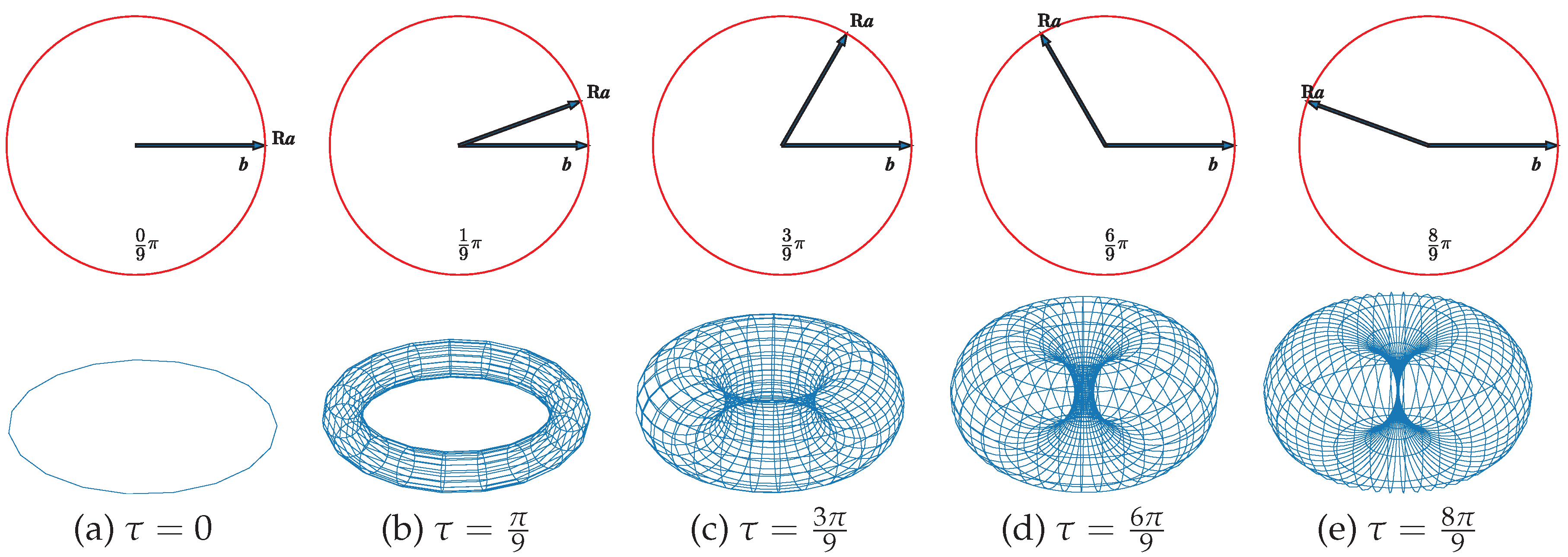
Figure 3.
The geometric relationship of one rotation constraint and its solution .
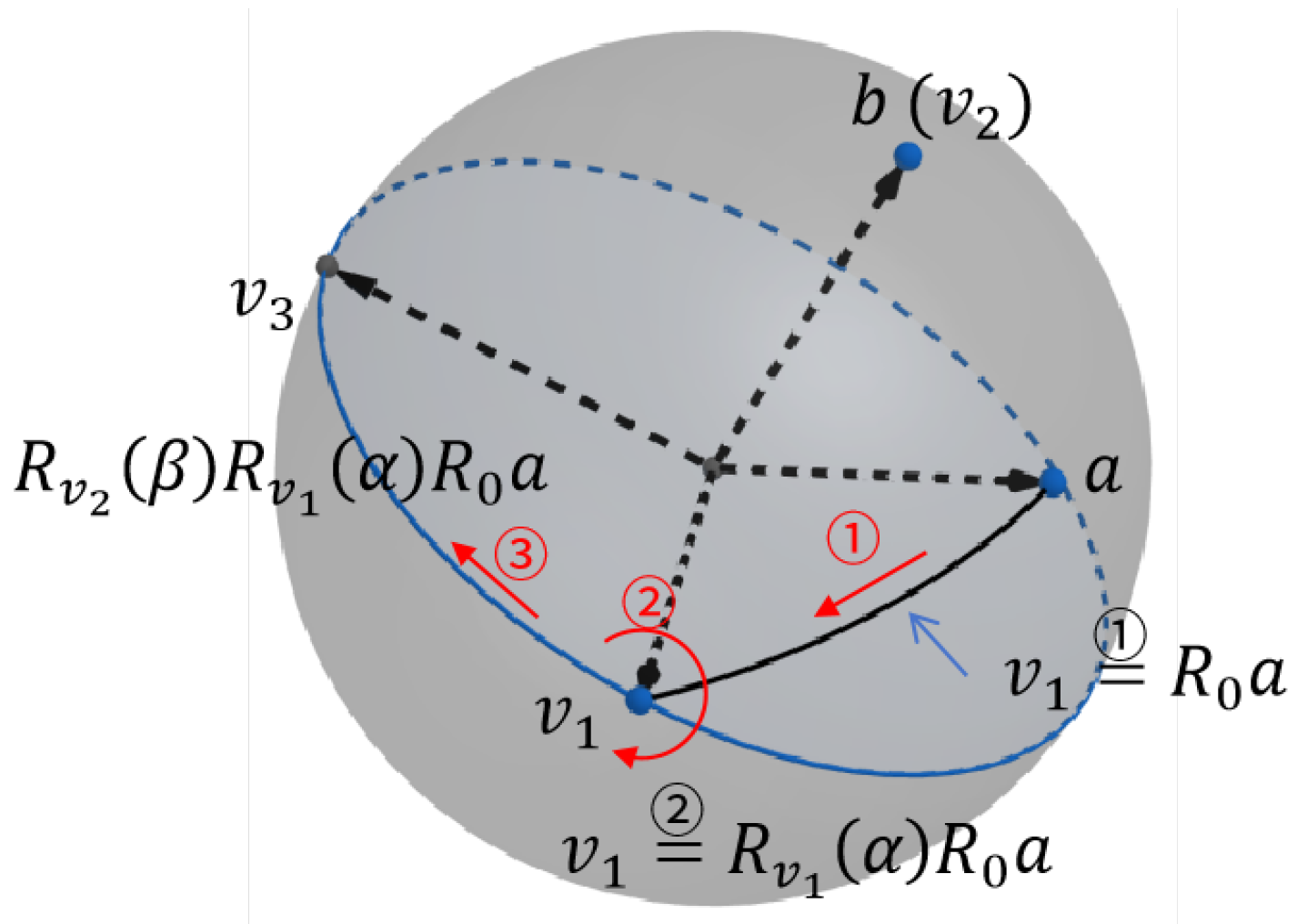
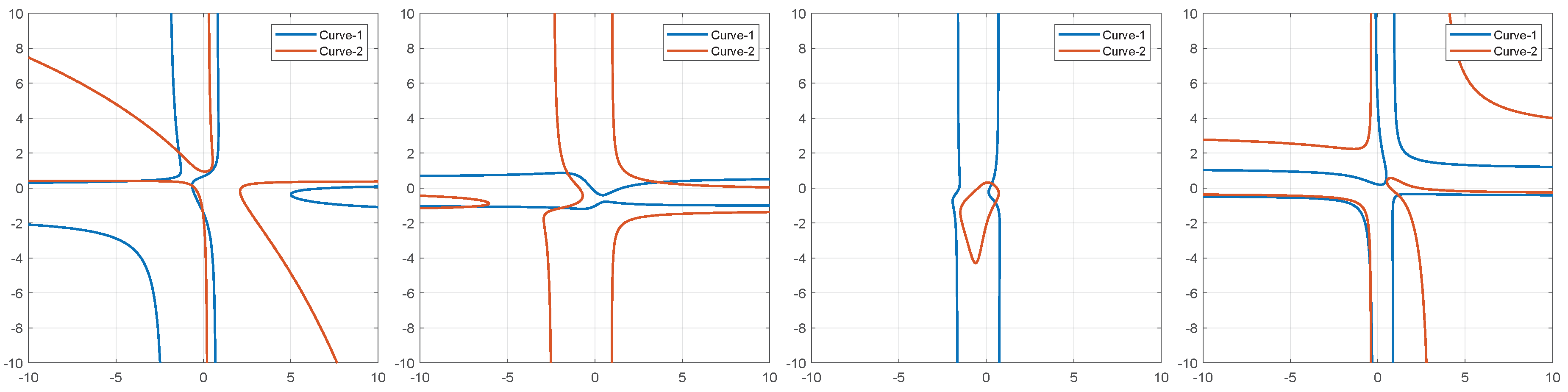
Figure 4.
The illustration for intersection curves of two Clifford tori in by stereographic projection.
Figure 4.
The illustration for intersection curves of two Clifford tori in by stereographic projection.
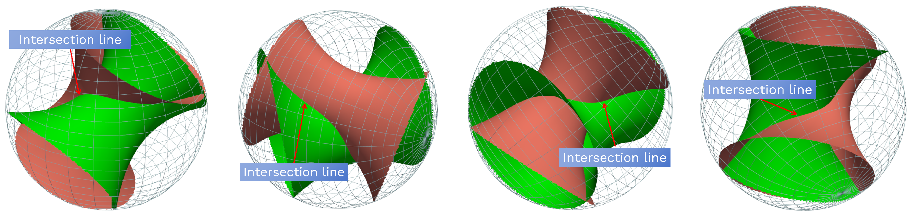
Figure 5.
The illustration for intersection curves of two Clifford tori in and space.
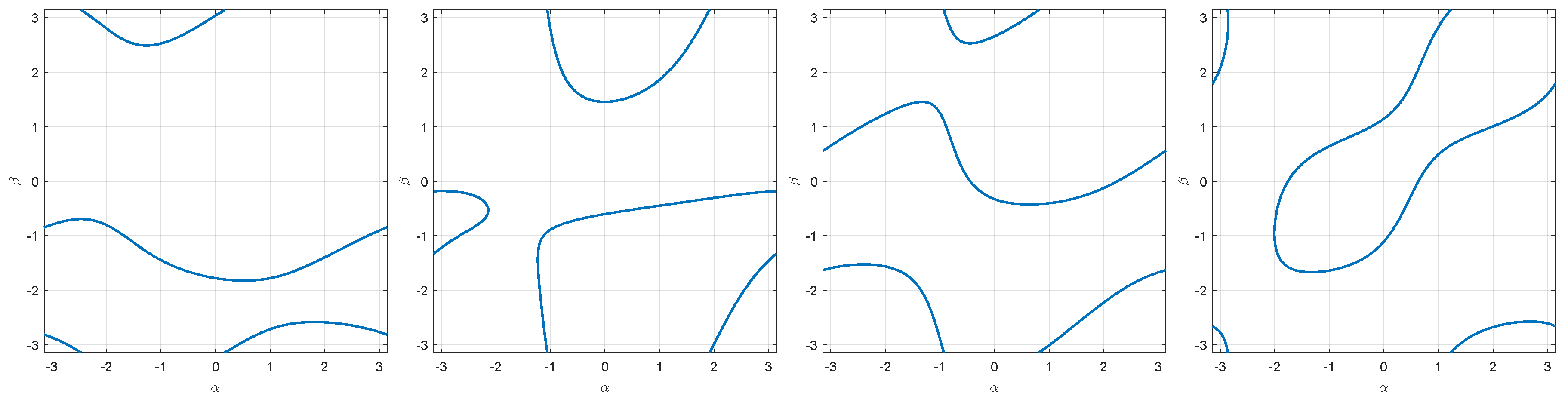
Figure 6.
The intersection of two curves that are constructed by rotation constraints in the 2D plane. Specifically, we can consider and as two surfaces in . Let , it means plane and it cuts the surfaces and . Consequently, there are two intersection lines, which can be drawn in plane.
Figure 6.
The intersection of two curves that are constructed by rotation constraints in the 2D plane. Specifically, we can consider and as two surfaces in . Let , it means plane and it cuts the surfaces and . Consequently, there are two intersection lines, which can be drawn in plane.
Disclaimer/Publisher’s Note: The statements, opinions and data contained in all publications are solely those of the individual author(s) and contributor(s) and not of MDPI and/or the editor(s). MDPI and/or the editor(s) disclaim responsibility for any injury to people or property resulting from any ideas, methods, instructions or products referred to in the content. |
© 2025 by the authors. Licensee MDPI, Basel, Switzerland. This article is an open access article distributed under the terms and conditions of the Creative Commons Attribution (CC BY) license (http://creativecommons.org/licenses/by/4.0/).
Copyright: This open access article is published under a Creative Commons CC BY 4.0 license, which permit the free download, distribution, and reuse, provided that the author and preprint are cited in any reuse.


