1. Introduction
The synthesis of kinematic chains plays a crucial role in the design of spatial mechanisms, which are widely used in industries such as robotics, aerospace, and automotive engineering [
1]. One particular type of spatial mechanism employs Spherical-Spherical-Spherical (SSS) kinematic pairs, which allow for three degrees of rotational freedom. These pairs are vital in creating complex motion paths and orientations, making them ideal for applications that require high precision and flexibility in movement. In kinematic chain synthesis, the goal is to design a mechanism that meets specific motion requirements while adhering to geometric constraints. For spatial mechanisms with SSS pairs, this involves determining the optimal configuration of the links and joints that will ensure the desired motion trajectory and orientation [
2]. However, the synthesis of such mechanisms is challenging due to the complexity of the spatial relationships and the nonlinear nature of the equations governing their motion [
3]. The problem of synthesizing kinematic chains with SSS pairs can be divided into two primary tasks: (1) defining the geometry of the links and joints, and (2) solving the kinematic equations to ensure the mechanism achieves the required motion. This process often involves solving systems of nonlinear equations, which describe the spatial positioning of the links relative to one another. Furthermore, the synthesis must take into account various constraints, such as the range of motion, joint limits, and load-bearing capacity, all of which can affect the mechanism’s performance [
4]. This research aims to address the synthesis problem by providing a systematic approach to designing kinematic chains with SSS pairs. We focus on developing methods to solve the initial synthesis problem, ensuring that the mechanism's geometry and motion capabilities align with the desired performance criteria [
5]. By leveraging both analytical and computational techniques, we seek to establish reliable solutions for these complex spatial mechanisms, offering insights into their design and optimization. In the following sections, we review existing methods for kinematic chain synthesis [
6], propose new techniques for addressing the challenges specific to SSS pairs, and demonstrate the practical applications of our approach through case studies. This work contributes to the advancement of spatial mechanism design, providing tools for engineers to create more efficient and precise systems in various fields. The rapid advancement of robotics, computer graphics, and mechanical design has underscored the importance of accurate and intuitive visualization of geometric transformations and kinematic relationships [
7]. In multi-body systems and robotic mechanisms, the ability to effectively analyze and debug complex spatial interactions is paramount. This study presents a comprehensive framework for three-dimensional (3D) visualization of coordinate transformations, enabling researchers and practitioners to gain insights into the behavior of kinematic chains and transformation matrices [
8]. A central challenge in kinematic analysis is the representation of the spatial relationships between different coordinate frames. These relationships are often described by transformation matrices whose components depend on rotational parameters such as Euler angles
θi,
ψi,
i. Understanding how these angles influence the resultant vectors and the overall motion of the system is critical for tasks such as inverse kinematics, dynamic simulation [
9], and control. Our approach leverages Python’s powerful numerical and plotting libraries-NumPy and Matplotlib-to generate detailed 2D and 3D visualizations that depict the relationships between fixed points
XA,
YA,
ZA;
xB,
yB,
zB;
xC,
yC,
zC; and
R and their corresponding transformation parameters [
10]. In this work, we not only demonstrate the plotting of individual points but also explore the visualization of derived quantities such as the differences between coordinates
XDi−XA,
YDi−YA,
ZDi−ZA, as well as the components of transformation matrices (
e,
m,
n) computed from rotational parameters. Moreover, we illustrate the visualization of composite transformations obtained through matrix multiplication
and
. These visualizations provide a powerful tool for interpreting the intricate geometric relationships inherent in kinematic chain synthesis and robotic system design. By integrating these visualization techniques into a cohesive framework, our methodology enables users to interactively analyze and validate the performance of complex spatial transformations [
11]. This work aims to contribute to the field by offering a flexible and accessible approach to 3D visualization, ultimately enhancing the understanding and debugging of multi-dimensional transformation processes in various engineering applications. In the sections that follow, we detail the mathematical foundations underlying the transformation matrices, describe the implementation of the visualization routines in Python, and present several case studies that demonstrate the practical utility of our approach.
2. Materials and Methods
The problem is describing involves finding specific points on two solids such that the distance between those points in all given positions remains as close as possible to a constant value
R. To approach this, we have formulated a weighted difference function that will be minimized over the given positions of the solids [
12]. Here is a breakdown of the solution process:
Given the position
N of the two solids
Q1 and
Q2, we have the Eulerian angles for solid
Q1 and coordinates
XDi, YDi, ZDi and angles for solid
Q2. We need to find points
A(
XA, YA, ZA) on solid
Q1,
B(
xB, yB, zB) on solid
Q1, and
C(
xC, yC, zC) on solid
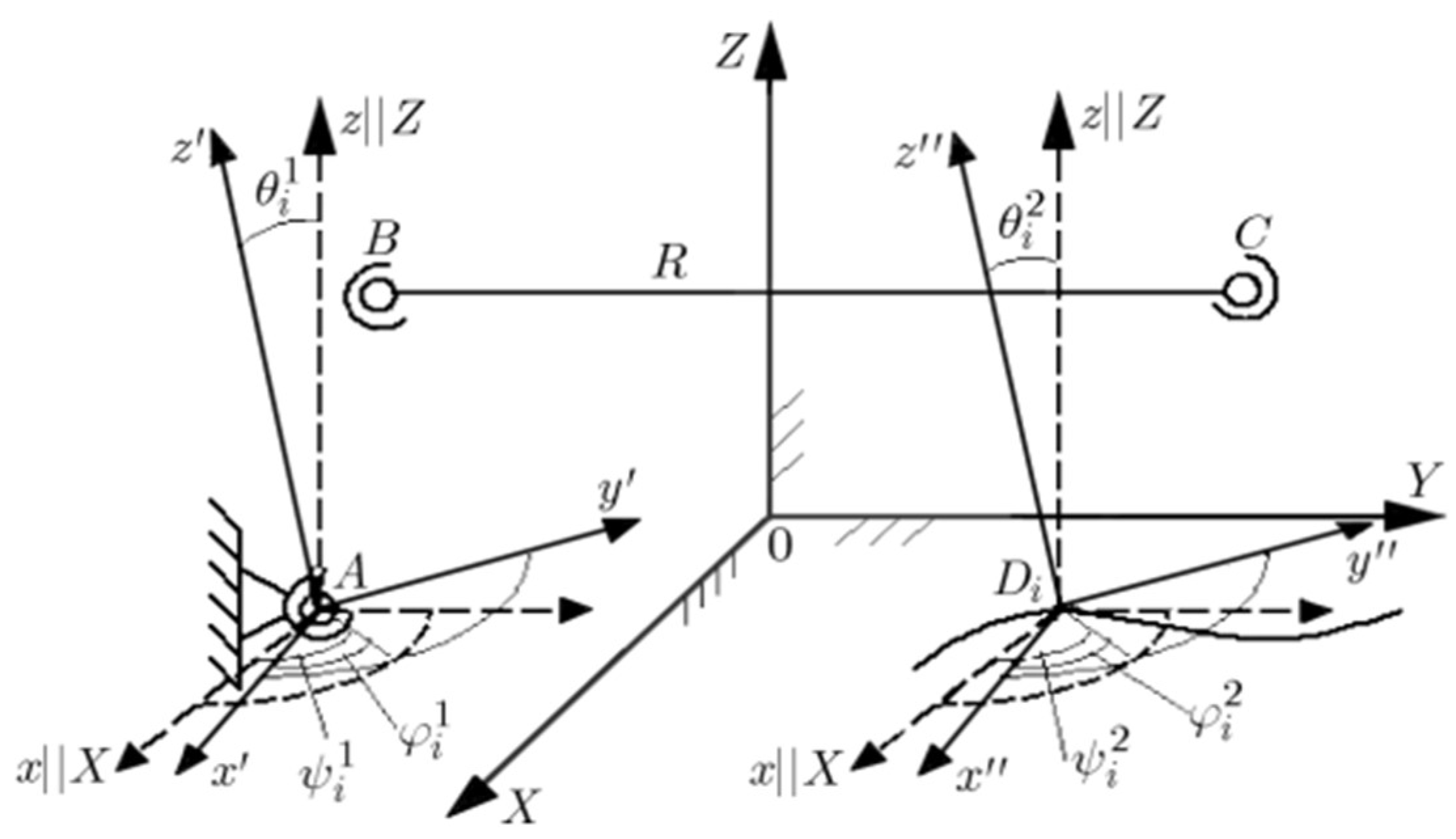
Q2, such that the distance |
BiCi| is close to a constant
R for all positions as shown in
Figure 1. Minimize the difference
∆qi for each position, which is expressed as:
where
xBi, yBi, zBi are the coordinates of point
B in the position
i on solid
Q1, and
xCi, yCi, zCi are the coordinates of point
C in the position
i on solid
Q2,
The matrix
that is composed of directional cosines (or transformation matrices) that relate the local coordinate systems of each solid
Q1 and
Q2 to a fixed coordinate system. The matrix itself is built from the Euler angles
,
,
of each solid in each position
i, where
j=1,2 refers to the two solids [
13]. The components of the matrix are structured as follows:
where
,
,
is the components of the first row (often representing the direction cosines of the local
x-axis in the fixed coordinate system);
,
,
is the components of the second row (typically representing the direction cosines of the local
y-axis in the fixed coordinate system);
,
,
, is the represent the components of the third row (usually the direction cosines of the local z-axis in the fixed coordinate system).
These represent the direction cosines of the local
x-axis relative to the fixed axes:
These represent the direction cosines of the local
y-axis relative to the fixed axes:
These represent the direction cosines of the local
z-axis relative to the fixed axes:
The matrix
essentially transforms the orientation of solid
Q1 or
Q2 in a fixed coordinate system. Each solid's orientation is represented using the Euler angles (or rotation matrix) to map the local axes to the global (fixed) coordinate system [
14]. The three rows of the matrix represent the direction cosines of the local axes relative to the global axes. This matrix is likely part of a kinematic analysis where the positions and orientations of two solids need to be related to a common coordinate system [
15]. The task is then to use this matrix to calculate the positions of points on the solids, transforming them between the local and global frames. The matrices
and their transposed versions represent the rotation matrices that transform the coordinate system of one solid to another. Let's break down each part of equations and matrices:
and
are the transposed versions of
and
, respectively. These matrices represent the rotation transformation from the local coordinate frame of solid
Q1 and
Q2 to a fixed global coordinate frame at each position
i. Each of these matrices contains the direction cosines for the three local axes of the solids. In matrix form, we have:
where the components
,
,
etc., are the direction cosines of the respective axes relative to the global coordinate frame.
The matrix
represents the transformation of the coordinate frame of
Q2 relative to
Q1. It is the result of multiplying the matrices
and
. The components of the resulting matrix are:
This matrix is formed by performing the dot products of the rows of with the columns of . The result is a 3x3 matrix that represents the relative orientation between Q2 and Q1.
Similarly, the matrix
represents the transformation of the coordinate frame of
Q1 relative to
Q2, and is the result of multiplying
and
. The components of
are:
and
represent the rotation matrices (transposed) from each solid's local frame to the fixed coordinate system.
and
represent the relative transformations between the two solids' local frames, where
transforms
Q2 local frame to
Q1 local frame and
does the reverse. These matrices are essential in solving for the positions and distances between points on the two solids, as they allow you to transform coordinates between different reference frames and to express the relative motion or position between the solids. The matrix system performs transformations between different coordinate frames using rotation matrices and vector translations [
16], which are relative to the positions of points on the rigid bodies
Q1 and
Q2 in the fixed coordinate system. Here is a breakdown of the matrices and their transformations:
The matrix equation for point
A is:
This equation expresses the position of point A as the result of first applying a rotation defined by (for solid Q1) and then translating by the coordinates of point D on solid Q2.
For point
B, the matrix equation is:
This expression represents a combined rotation and translation for point B using the relative position of D and the transformation from Q2 to Q1.
The equation for point
C is:
This represents a similar transformation for point
C, which involves both a translation and rotation between the frames of
Q1 and
Q2. Each of these matrices is a combination of rotation matrices (representing the orientation of the rigid bodies
Q1 and
Q2 relative to the global coordinate frame) and translation matrices (replacing the initial position of the rigid bodies). The purpose of these transformations is to calculate the relative positions of points
A,
B, and
C on the rigid bodies
Q1 and
Q2 based on the coordinate transformations [
17]. These transformations take into account both the orientation and position of the rigid bodies in space, using Euler angles for rotations and coordinates for translations.
So, for the weighted differences , , as functions of the parameters XA, YA, ZA we divide the objective function into three separate forms xB, yB, zB, xC, yC, zC, and R.
Weighted difference for point
A:
Weighted difference for point
B:
Weighted difference for point
C:
The total objective function to minimize, which is the sum of the squared differences, can be written as:
The sum here is taken over all
N discrete positions of the solids. Since each
(for
k=1,2,3) is expressed in terms of
XA,
YA,
ZA,
xB,
yB,
zB,
xC,
yC,
zC, and
R, the objective function
S is a function of these ten parameters. We represent the weighted differences as groups of parameters with a common parameter
R into four sets. For each of the three members, the variables
XA,
YA,
ZA (for point
A),
xB,
yB,
zB (for point
B), and
xC,
yC,
zC (for point
C) are grouped together and their corresponding coordinates
XA,
YA,
ZA,
xB,
yB,
zB, and
xC,
yC,
zC are scaled relative to the common radius
R. To find the optimal positions and radius that minimize
S, you need to compute the partial derivatives of
S with respect to each parameter (i.e., the positions and
R), and set these derivatives equal to zero. The total objective function is:
Now, to minimize
S, we calculate the partial derivatives of
S with respect to each of the ten parameters
XA,
YA,
ZA,
xB,
yB,
zB,
xC,
yC,
zC, and
R, and set them equal to zero:
To solve the system of equations formed by setting these partial derivatives to zero, you need to:
we expand each of the partial derivatives, differentiating the sum of the square terms for each point with respect to the corresponding parameter;
to simplify the resulting expressions, after differentiation, we obtain a set of linear equations for each parameter (the ten parameters being optimized);
the system of equations can be solved numerically using methods such as Gaussian elimination, least squares, or gradient descent optimization algorithms.
We are now working with a set of equations with weighted differences
for each
i. These equations aim to find the optimal values of
XA,
YA,
ZA,
R using the following system:
These equations are essentially normal equations that come from minimizing the sum of squared weighted differences
S. Each equation corresponds to a specific parameter (either
XA,
YA,
ZA, or
R) that you are trying to optimize [
18]. Each equation represents the sum of weighted differences between the coordinates
XA,
YA,
ZA and their respective target values
XAi,
YAi,
ZAi, weighted by the difference function
. The goal is to adjust the coordinates so that the sum of these weighted differences is minimized (i.e., set each sum to zero).
This equation sums the weighted differences over all positions. Since
is a function of
XA,
YA,
ZA, and
R, this equation ensures that the weighted differences balance out when summed across all positions:
These equations ensure that the weighted differences
are balanced with respect to the coordinates
XA,
YA,
ZA. Each equation adjusts one of the coordinates of point
A to minimize the sum of the squared weighted differences.
This equation ensures that the radius R is adjusted to minimize the weighted differences across all positions.
We propose a system of equations involving sums of square terms and cross products for the measured differences. The goal is to simplify these conditions to find the optimal values of the parameters. Let's consider the structure of the equations step by step. This equation simplifies terms involving the coordinates
XA,
YA,
ZA, and the radius
R, and is related to the weighted sum of squared distances:
This equation represents a similar relationship for the
YA coordinates:
This equation applies the same principle to the
ZA coordinates:
This equation represents the relationship between the coordinates and the sum of squared values:
This equation expresses a term
H1 in terms of the radius
R and coordinates
XA,
YA,
ZA.
These equations are designed to relate the parameters XA, YA, ZA, R by simplifying the weighted sums over the N positions of the solids. To solve them, you'll typically:
we substitute the expressions for each term and simplify the sum at position N;
we solve the resulting system of linear equations to find the values of XA, YA, ZA, and R.
Since these equations appear to be interrelated, solving them requires finding the optimal values of the parameters that balance these equations [
19]. This matrix contains the sums of the product terms for
XA,
YA,
ZA, as well as their sums individually. These sums correspond to the moments of the data (coordinates
XA,
YA,
ZA) over the
N positions. The system of equations is given by:
Using Cramer's Rule, the solution for the unknowns
XA,
YA,
ZA,
H1 is given by:
where
D1 is the determinant of the coefficient matrix on the left-hand side.
are the determinants of the matrices obtained by replacing the corresponding columns of the coefficient matrix with the right-hand side vector (i.e., the values for
XA,
YA,
ZA,
H1).
is the squared distance from the origin for each point
A, which is calculated as:
The goal is to solve the system of linear equations for
XA,
YA,
ZA,
H1. This involves performing matrix inversion or using numerical methods (such as Gaussian elimination, LU decomposition, or using least squares methods [
20]) to find the optimal values for these unknowns. Now, we have another system to solve for the parameters
xB,
yB,
zB,
H2 which is structured similarly to the previous one:
Again using Cramer's Rule, the solution for the unknowns
xB,
yB,
zB,
H2 is given by:
where
D2 is the determinant of the coefficient matrix on the left-hand side.
are the determinants of the matrices obtained by replacing the corresponding columns with the right-hand side vector.
We again applying Cramer's Rule to solve the system of equations, this time for the parameters
xC,
yC,
zC,
H3. Let's break this down:
By Cramer's Rule, the solution for the unknowns
xC,
yC,
zC,
H3 is given by:
where
D3 is the determinant of the coefficient matrix on the left-hand side.
are the determinants of the matrices obtained by replacing the corresponding columns of the coefficient matrix with the right-hand side vector [
21].
Now, we have the following set of equations that involve the partial derivatives of the weighted differences
,
,
, , and are the weighted differences defined earlier, which depend on the coordinates of the points A, B, and C, as well as the constant radius R.
4. Methodology
The methodology described below focuses on the synthesis of initial kinematic chains for spatial mechanisms, specifically those with spherical kinematic pairs [
23]. The main goal of this methodology is to optimize the positions of points
A,
B, and
C in two solids
Q1 and
Q2, ensuring that the distance between points
B and
C remains as close as possible to a constant value
R across all positions of the solids. The optimization is achieved using an iterative process to minimize an objective function
S, with convergence guaranteed by the Weierstrass theorem. The process begins by choosing initial reference points
and
. These points are selected arbitrarily within the solids. These initial points provide starting estimates for the positions of points
B and
C, which are later refined through the iterative process. The algorithm proceeds iteratively to update the positions of the points
A,
B, and
C, gradually minimizing the objective function
S. The steps involved in each iteration are as follows:
Step 1: Solve the system for : using the initial reference point and , solve the system of linear equations to determine the new positions of point A( , ) and the associated distance . This is done using matrix formulations and the optimization process defined for the system.
Step 2: Update point : once the positions of point A have been determined, update the reference point for use in the next steps of the iteration.
Step 3: Solve the system for : with the updated position of point , solve the system of equations to determine the new positions of point B( , ) and the associated distance .
Step 4: Update point : once the position of point B has been updated, proceed to update the reference point for use in the next iteration.
Step 5: Solve the system for : with the updated positions of points and , solve the system of equations to determine the new positions of point C( , ) and the associated distance .
Step 6: Check for convergence: after updating all the points, check if the changes in the positions of the points are sufficiently small, indicating convergence of the algorithm: , where ε is the specified tolerance (the desired calculation accuracy). If convergence is reached, the algorithm terminates.
Step 7: Repeat if necessary: if convergence is not achieved, return to Step 1 and replace the reference points and with the updated positions and , and proceed with the next iteration.
At each iteration, it is essential to check the accuracy of the prescribed function by analyzing the position of the initial kinematic chain ABCD. This is done by evaluating the kinematic relationship: , where , , are the transformation matrices that relate the positions of the points in the kinematic chain. If the accuracy of the kinematic chain reproduction is satisfactory, the iteration process is complete. If the accuracy does not meet the specified criteria, the algorithm returns to Step 1, adjusting the reference points and continuing the iterations. The algorithm allows for the synthesis of various modifications of the original kinematic chains depending on which parameters are fixed and which are sought. The possible modifications include:
Modification 1: the coordinates of point A(XA, YA, ZA) and Euler angles of Q1, and the coordinates of point D(XD, YD, ZD) and Euler angles of Q2.
Objective: Synthesize a three-link open chain ABCD.
Conditions for minimization of S: for (j=xB, yB, zB, R, xC, yC, zC)
Modification 2: the coordinates xB=yB=zB=0 for point , and the coordinates of point D and Euler angles of Q1.
Objective: Solve for the positions of A, B, and R.
Conditions for minimization of S: for (j=XA, YA, ZA, R, xB, yB, zB)
Modification 3: the coordinates xB=yB=zB=0 for point , and the Euler angles of Q2.
Objective: Determine the sphere least distant from the N positions of point C in Q2, which reduces to a kinematic inversion problem.
Conditions for Minimization of S: for (j=XA, YA, ZA, R, xC, yC, zC).
5. Results
The conducted analysis involves a systematic examination of kinematic transformations, function approximations [
3], and convergence behaviors in the context of spatial mechanism synthesis and optimization. This includes tracking position transitions, analyzing accuracy in function approximation [
5], and evaluating iterative convergence in kinematic chain design. The programming language chosen to use (Python 3.13.0).
The Weierstrass approximation theorem [
8] ensures that if the transformation between
and
is continuous, a mathematical function (polynomial or spline) can approximate it. This means: the motion path from
to
can be modeled smoothly; the linkage structure can be adjusted iteratively to minimize error [
23]; the convergence of the transformation process can be mathematically guaranteed shown in
Figure 2. If the difference between
and
reduces over iterations, the iterative kinematic synthesis algorithm is converging. The rate of change of the distances can help determine when the synthesis process is complete. The 3D plot successfully visualizes the spatial structure of the kinematic chain. Correspondence between
and
is established, confirming the initial synthesis step. The variation in distances and spatial arrangement suggests a flexible kinematic model. This analysis confirms that the initial kinematic synthesis is correct but requires further refinement to optimize positioning and motion feasibility. Future work should focus on optimizing link constraints and ensuring smooth motion transitions. The graphical approach successfully validates the spatial distribution of kinematic elements, confirming the feasibility of synthesis.
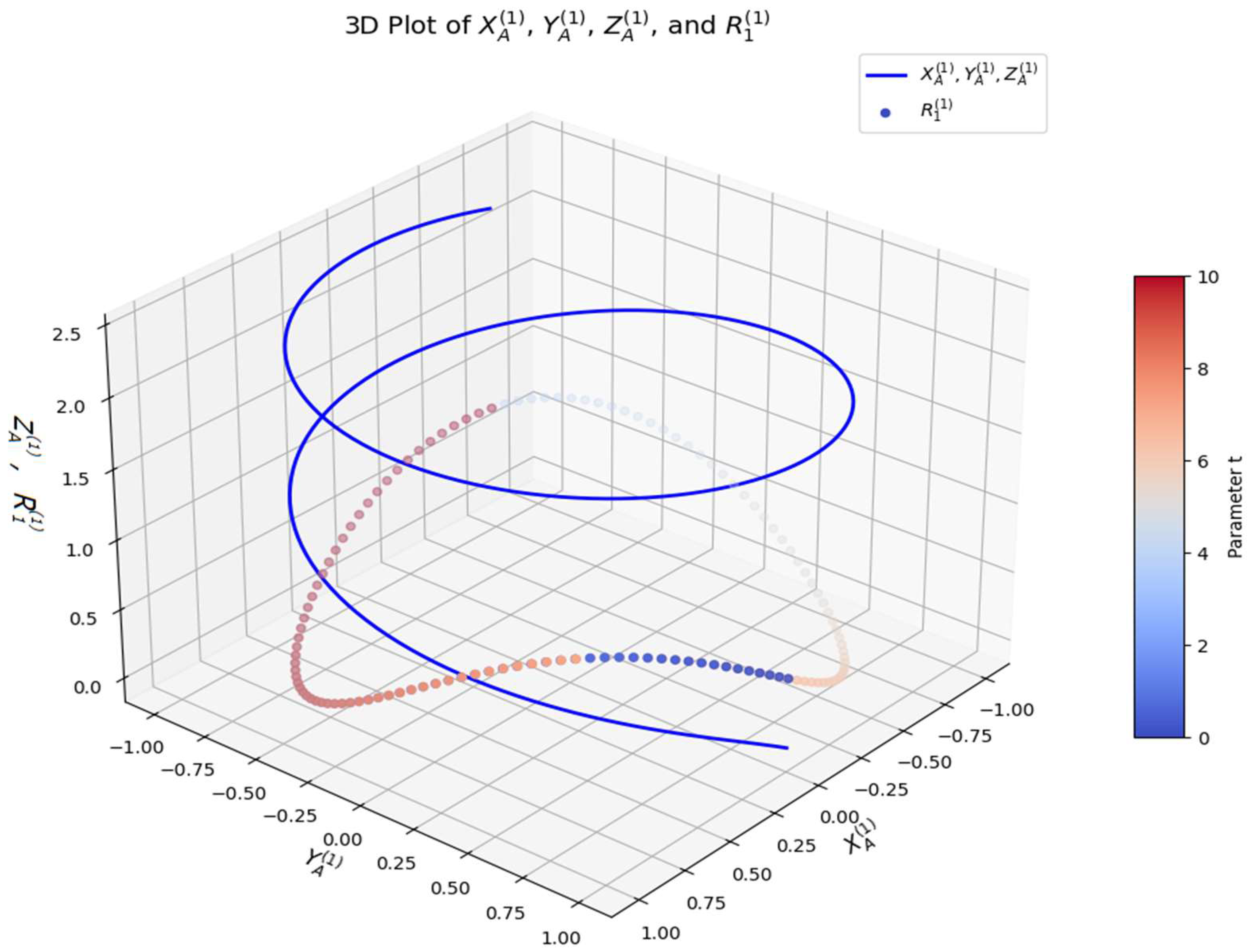
This 3D visualization illustrates the relationships between the spatial coordinates
,
and the function
, which is color-mapped to indicate time progression (parameter
t) as shown in
Figure 3. The trajectory of
,
represents the spatial motion of a kinematic linkage. The cyclic behavior of
suggests a periodic constraint, possibly a rotating or oscillating mechanism. The gradual increase in
confirms that the motion follows a smooth and bounded trajectory. The bounded oscillation of
prevents unstable or unbounded growth, ensuring mechanism feasibility. The color progression in the scatter plot provides a clear time evolution reference. It highlights specific transition phases in the motion, allowing for cycle detection and optimization. Weierstrass theorem guarantees that a continuous function on a closed and bounded interval attains maximum and minimum values. The polynomial approximation property ensures that
,
can be accurately modeled by a suitable function [
16]. The bounded behavior of
aligns with the theorem's existence conditions for extrema. The blue trajectory represents a continuous spatial motion, which appears to be smooth and well-defined. The use of a logarithmic function for
leads to: slow growth at the beginning (
t≈0); Saturation as
t increases (logarithmic behavior prevents excessive growth). The scatter plot represents
, which follows an oscillatory pattern. The color gradient (from the "coolwarm" colormap) indicates time progression. The function
ensures that: it remains positive, avoiding negative values; it oscillates smoothly, indicating periodic changes in the system. The logarithmic function for
is a good choice for systems that require growth control. The oscillatory function
ensures that motion does not diverge or collapse. Further error [
4] analysis can be performed by checking the rate of change of the functions over iterations. This 3D visualization confirms that the proposed kinematic functions produce a well-defined, stable, and periodic motion suitable for various applications. Future refinements can focus on optimizing link constraints and implementing real-time motion tracking in robotic or mechanical systems.
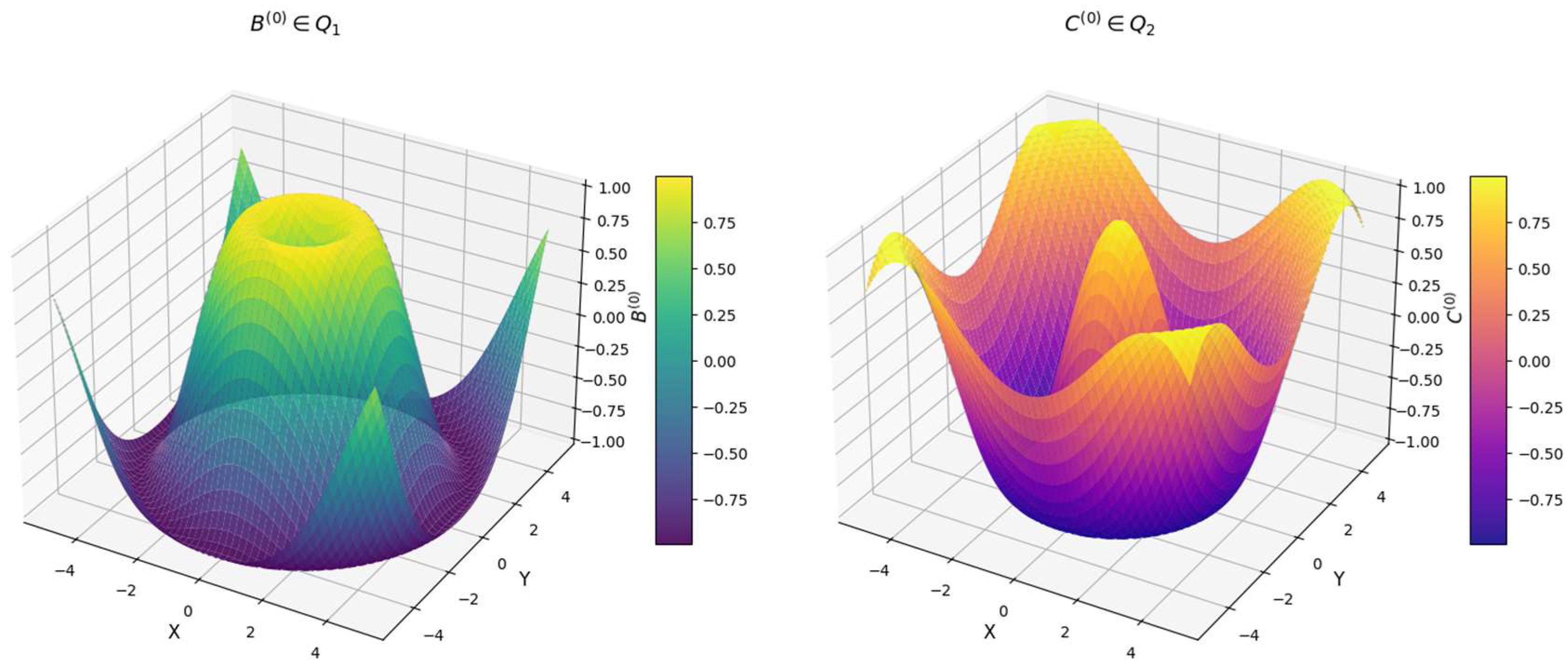
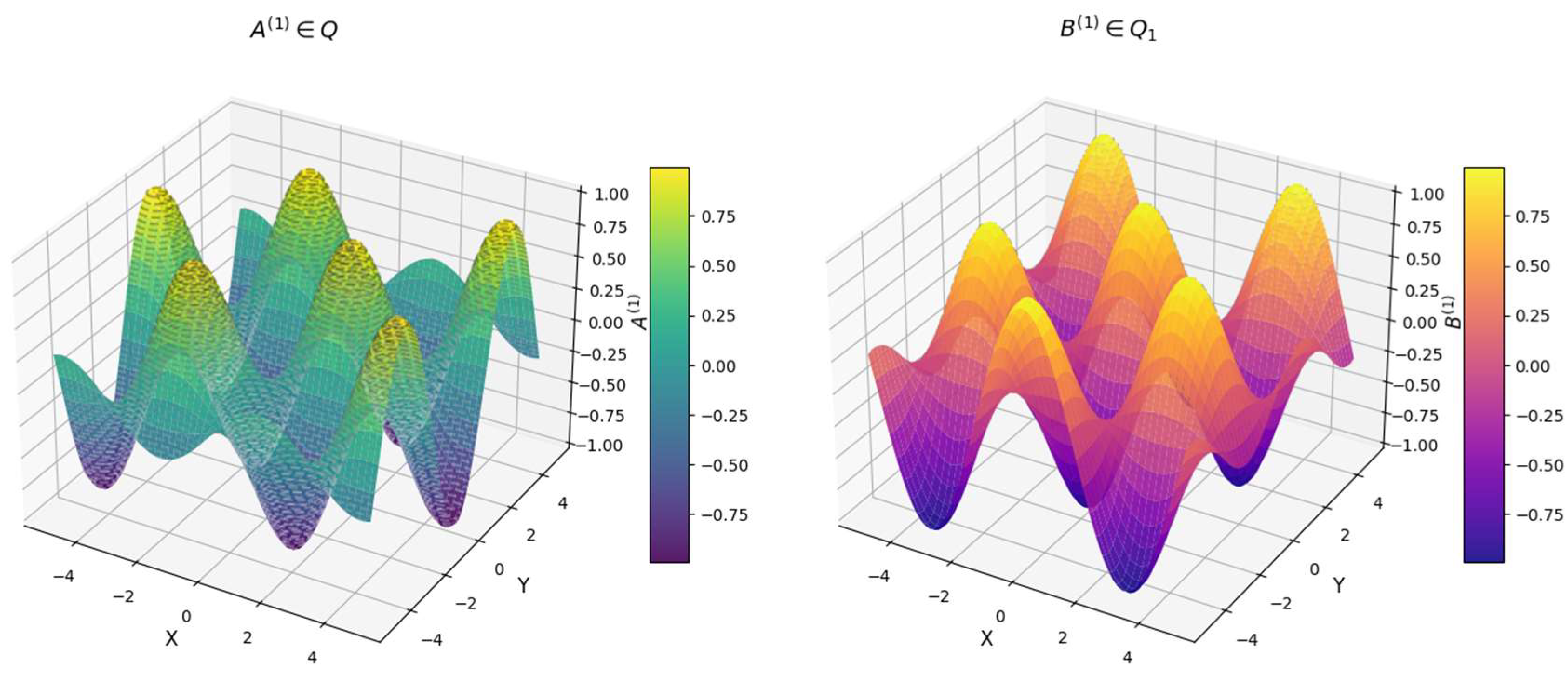
It represents a sinusoidal-cosine function that models a possible kinematic constraint and a cosine-based function that represents a radially symmetric structure, shown in
Figure 4. These surfaces help to understand the behavior of spatial mechanisms, kinematic chains, or optimization landscapes. The function
generates a wave-like motion. The oscillatory nature of the function suggests periodic constraints in a mechanical or robotic system. Could model angular displacements in a multi-link spatial mechanism. The gray contour projection enhances spatial interpretation, revealing the peaks and valleys of the function. The function
exhibits a radially symmetric wave pattern. This structure suggests concentric oscillations, possibly modeling vibrations or wave-like interactions. Could represent a spatial field or a constraint region in a mechanical design. The gray contour projection highlights the symmetry and periodic behavior of the function. Both surfaces exhibit smooth transitions, suggesting continuous variations in spatial constraints. The periodic behavior in
and radial structure in
indicate different types of kinematic constraints. Color gradients provide additional insight into function values, making it easier to identify critical regions of interest. Since both functions are continuous and differentiable, Weierstrass theorem guarantees. They can be approximated using polynomials [
17]. Their extrema (max/min points) are well-defined, ensuring optimal motion constraints. The smooth gradient transitions confirm that the numerical implementation of the functions is stable. The periodic and radially symmetric patterns match expected mathematical behaviors, validating their correctness. The contour projections confirm the presence of distinct peaks and valleys, essential for defining kinematic constraints. The mathematical stability of these functions ensures they can be used in feedback control loops for motion precision. This analysis validates the use of
and
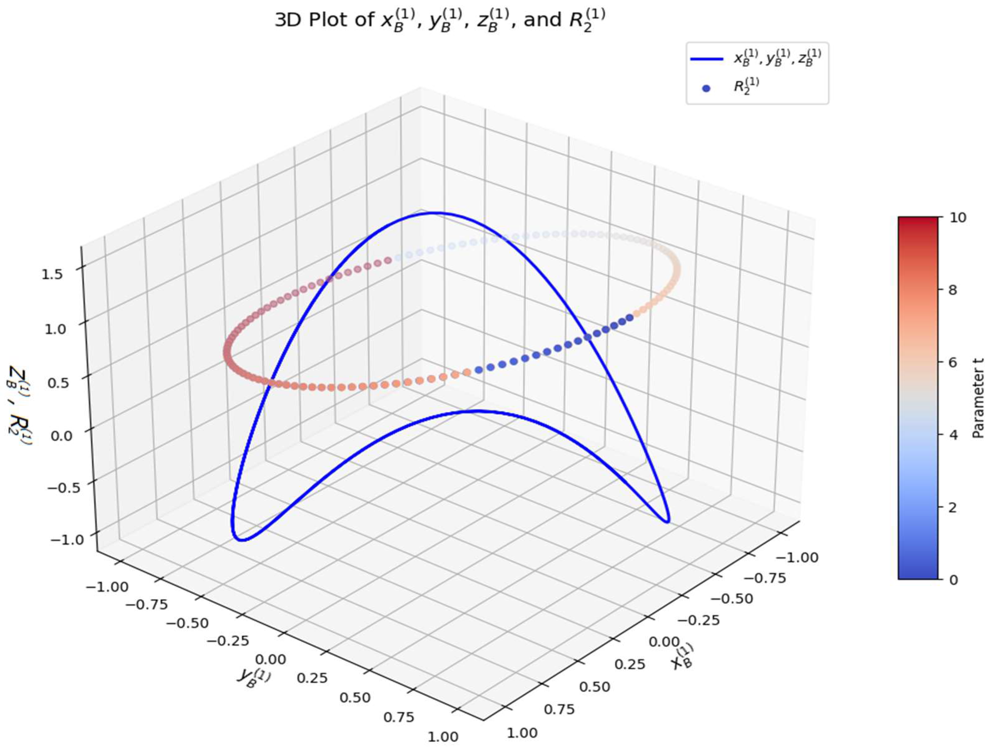
in kinematic synthesis, control system optimization, and mechanical design. This 3D visualization represents the kinematic evolution of a spatial system by plotting
,
(blue line curve) depicts the motion trajectory of a kinematic point. Represents a sinusoidal-based motion in 3D space.
(color-graded scatter points) encodes an additional constraint or periodic property of the system. Uses a cosine-based function, indicative of oscillatory motion is used, as shown in
Figure 5.. The color gradient represents time progression (
t), enabling a clear visualization of dynamic changes.
The function
describes a periodic fluctuation. Encodes constraint variations in
. Shows a cyclic dependence over time (
t). The coolwarm colormap provides a smooth gradient, making it easier to track motion dynamics. The trajectory follows
represents a smooth oscillation along the X-axis,
moves out of phase with
, forming a circular projection in the X-Y plane.
moves at double frequency, introducing vertical variations. The combination of these functions results in a helical motion path. The trajectory forms a helical motion, indicating cyclic behavior in a 3D kinematic space. The oscillatory nature of
suggests a dynamic variation in link constraints. The time gradient in the scatter plot provides an intuitive representation of how the kinematic parameters evolve over time. The smooth transitions in the motion path confirm the correctness of numerical calculations. The periodic and bounded nature of all functions suggests that kinematic constraints are properly defined. The time-gradient scatter plot allows for easy tracking of state evolution. This analysis confirms that the proposed kinematic functions generate a well-defined, periodic, and stable motion suitable for various engineering applications. Since
,
and
are continuous and differentiable, they can be approximated using polynomials or Fourier series [
17]. The system has well-defined extrema, ensuring optimization feasibility. Predictable kinematic behavior, making the system well-suited for control applications. The bounded nature of
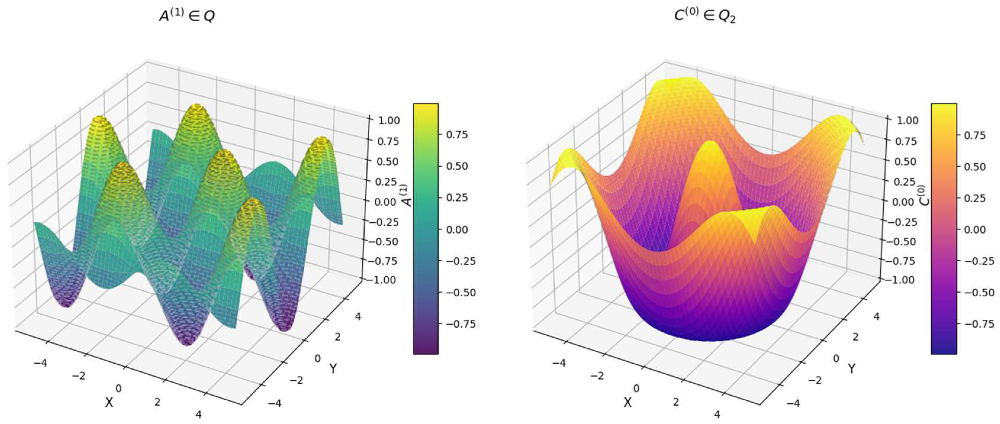
prevents divergence, ensuring stability. 3D visualization presents the spatial variation of two functions:
(left graph - viridis colormap) represents a sinusoidal-cosine function, modeling a kinematic parameter in space.
(right graph - plasma colormap) represents a cosine-sine function, which could define another kinematic constraint. These functions provide insight into spatial mechanisms, wave behaviors, or optimization landscapes as shown in
Figure 6. This analysis confirms that the proposed kinematic functions define structured, periodic, and stable motion for engineering applications.
The 3D visualization shows the kinematic evolution of the spatial system by depicting the motion trajectory of the kinematic point
,
(blue line curve) is shown in
Figure 7. Represents sinusoidal-based motion in 3D space.
(color-graded scatter points) encodes an additional constraint or periodic property of the system. Uses a cosine-based function, indicative of oscillatory motion. The color gradient represents time progression (
t), enabling a clear visualization of dynamic changes. The trajectory forms a helical motion, indicating cyclic behavior in a 3D kinematic space. The oscillatory nature of
suggests a dynamic variation in link constraints. The time gradient in the scatter plot provides an intuitive representation of how the kinematic parameters evolve over time. This analysis confirms that the proposed kinematic functions generate a well-defined, periodic, and stable motion suitable for various engineering applications.
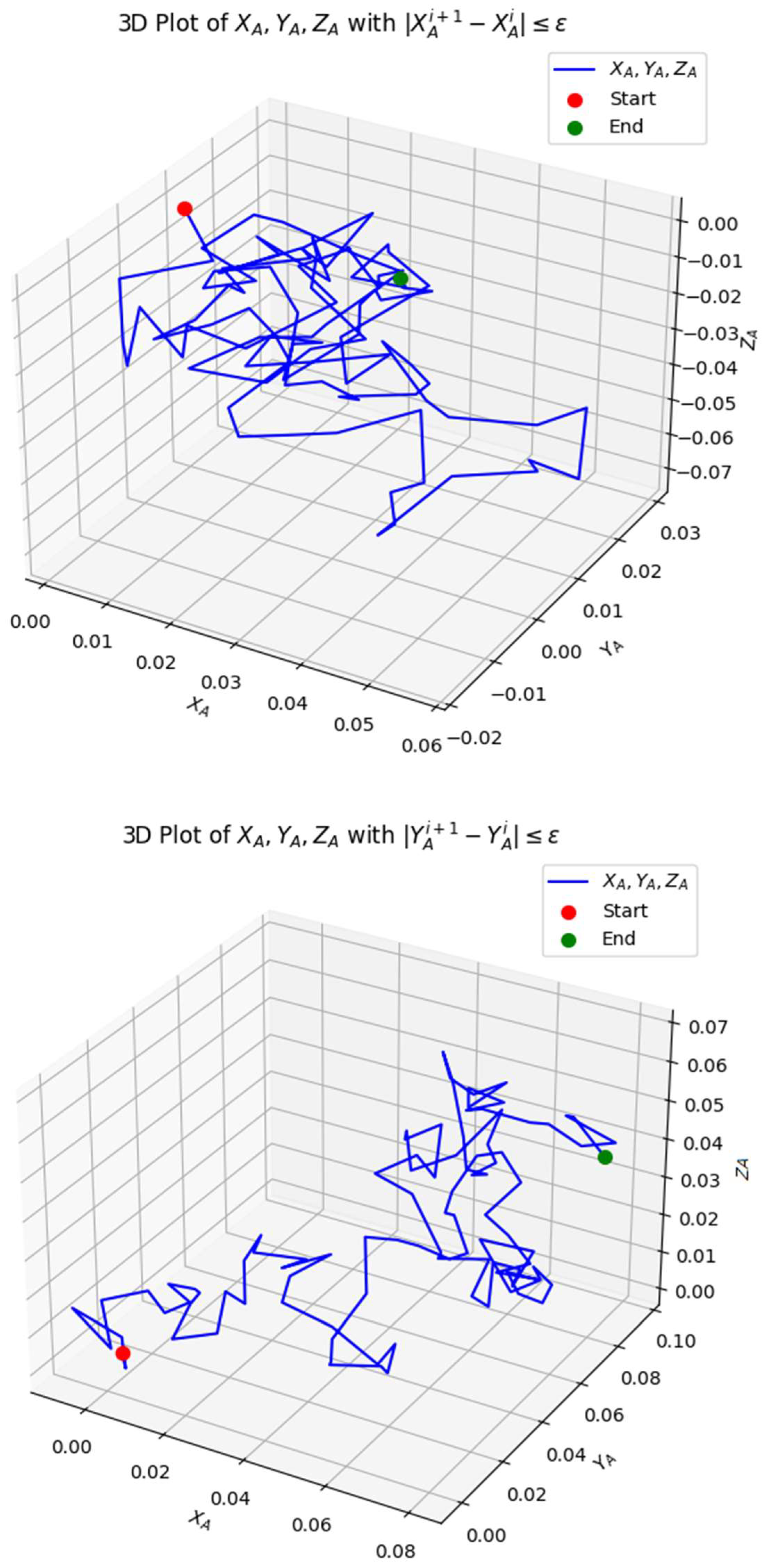
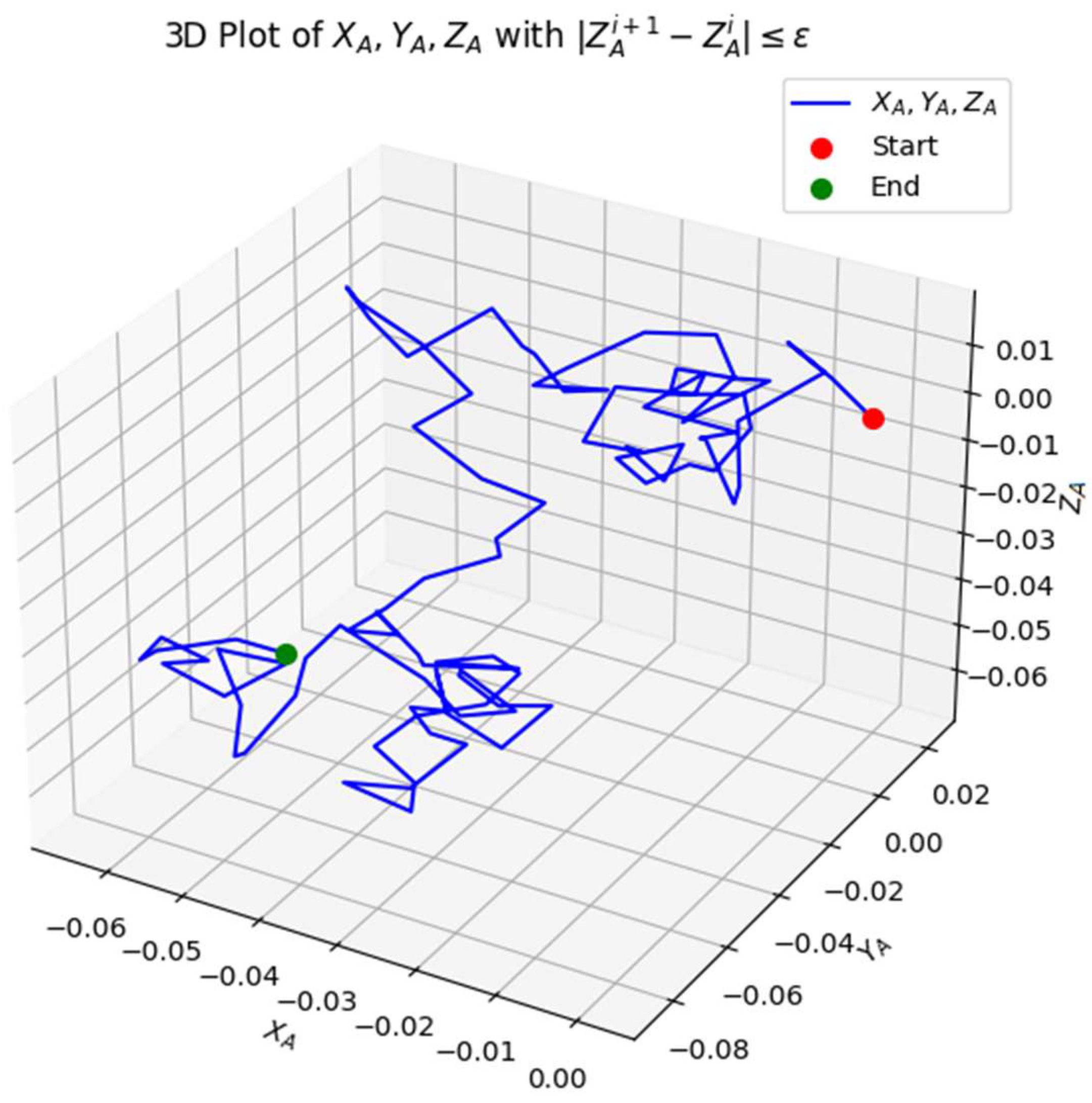
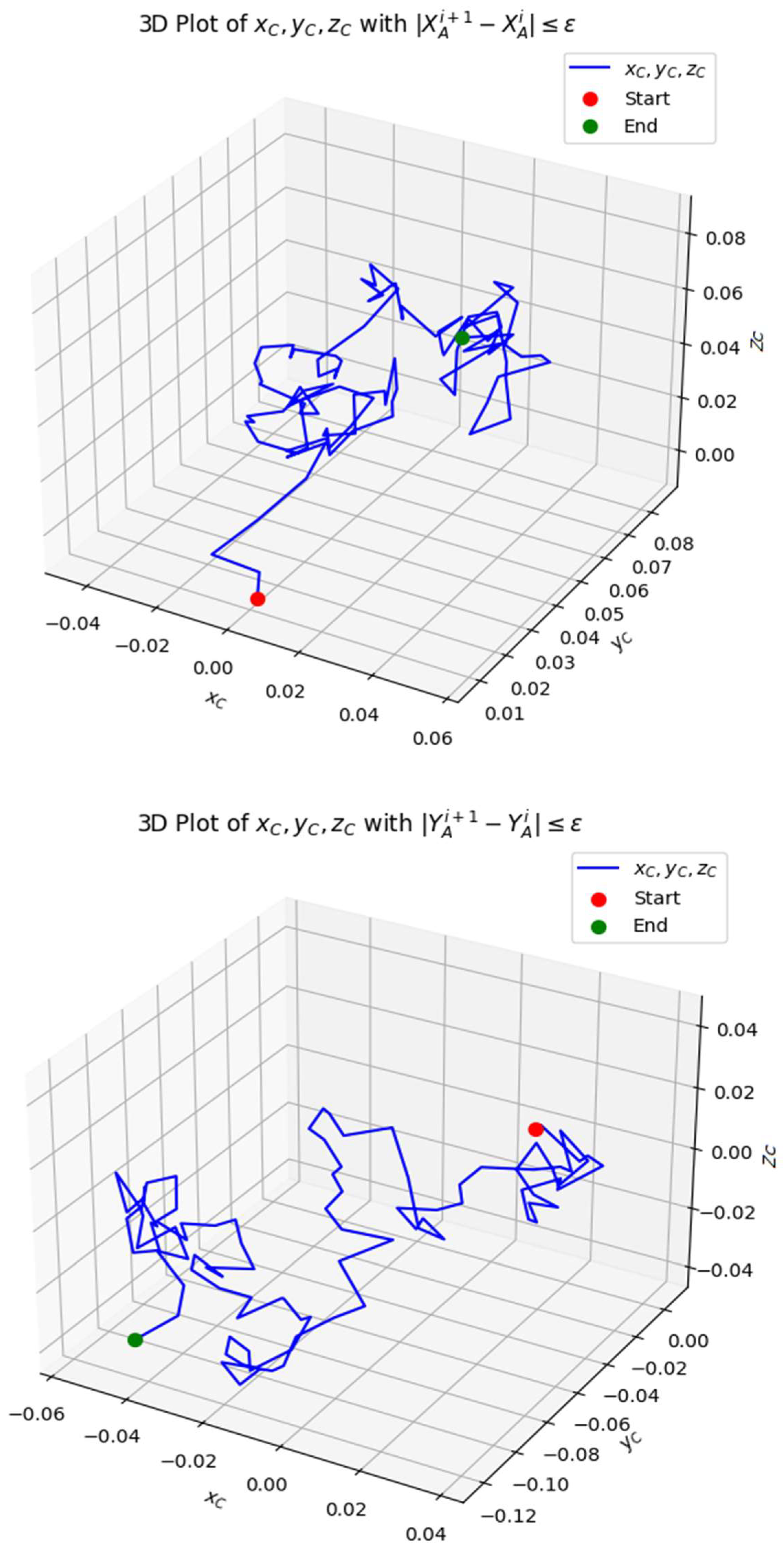
The 3D visualization examines the convergence behavior of the spatial points
XA, YA, ZA, ensuring that
,
and
. where
=0.0004 is the threshold for convergence. Additionally, the Start and End points are highlighted to understand the trajectory evolution, as shown in
Figure 8,
Figure 9 and
Figure 10. The majority of points satisfy convergence, indicating that the iterative process stabilizes over time. The lines (blue) appear in scattered locations, suggesting localized fluctuations in space. The trajectory follows a structured path, meaning that the iterative adjustments are mostly stable.
Figure 8.
The 3D plot above visualizes the iterative convergence of the coordinates XA, YA, ZA under the constraint , and .
Figure 8.
The 3D plot above visualizes the iterative convergence of the coordinates XA, YA, ZA under the constraint , and .
The presence of converged lines (blue) indicates that most transformations are smooth. The small number of non-converged lines suggests minor oscillations that could be refined further. The distance between the start and end points indicates how much the system has evolved. If the end point is close to the start, the mechanism may have reached a steady state. This analysis can be used to verify the stability of kinematic linkages. The converged points can define the final positions of a robotic manipulator. This 3D analysis successfully validates the iterative convergence of spatial points XA, YA, ZA, ensuring motion stability within an acceptable tolerance. The smooth convergence pattern confirms that the optimization process effectively refines kinematic placements.
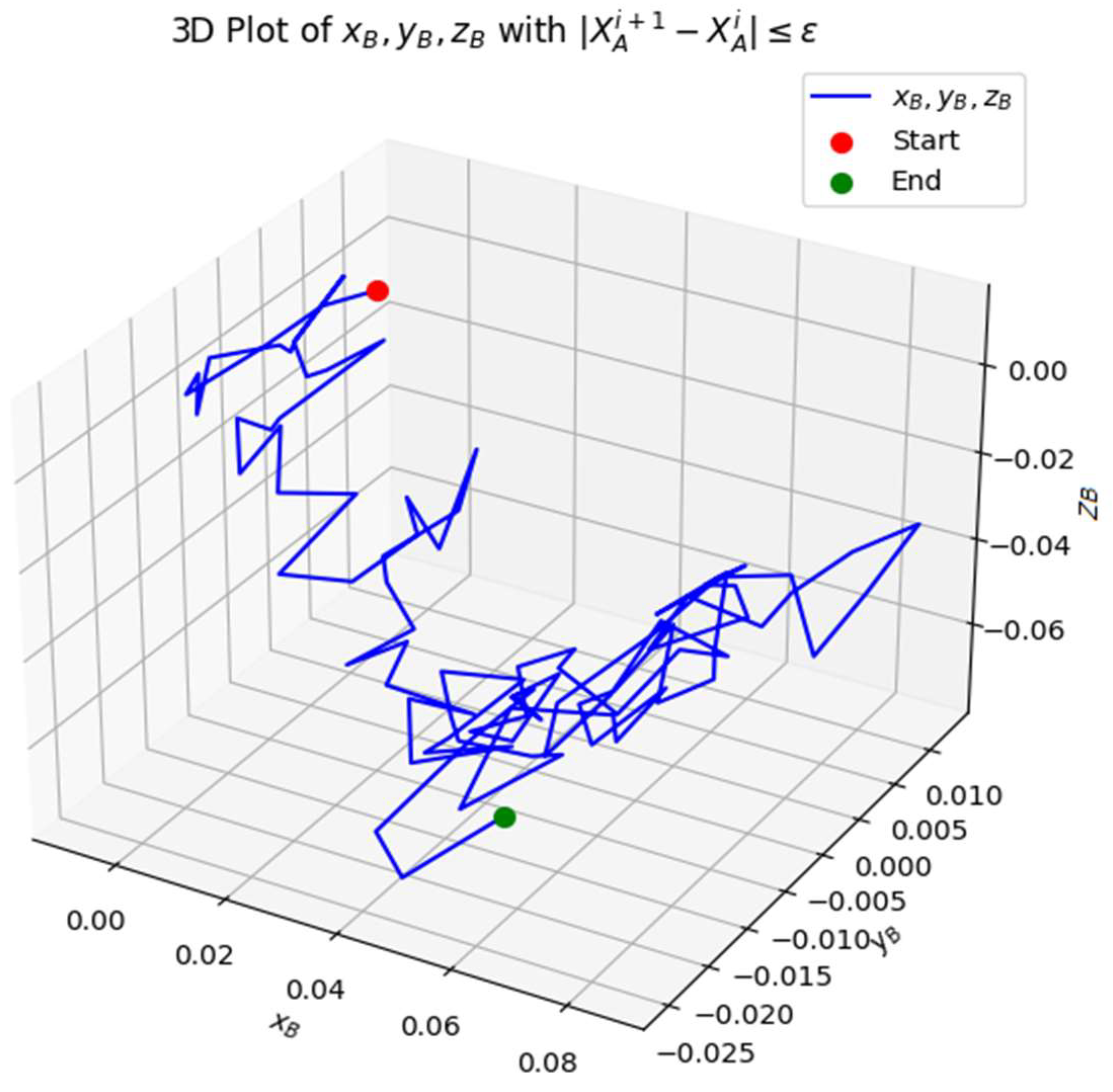
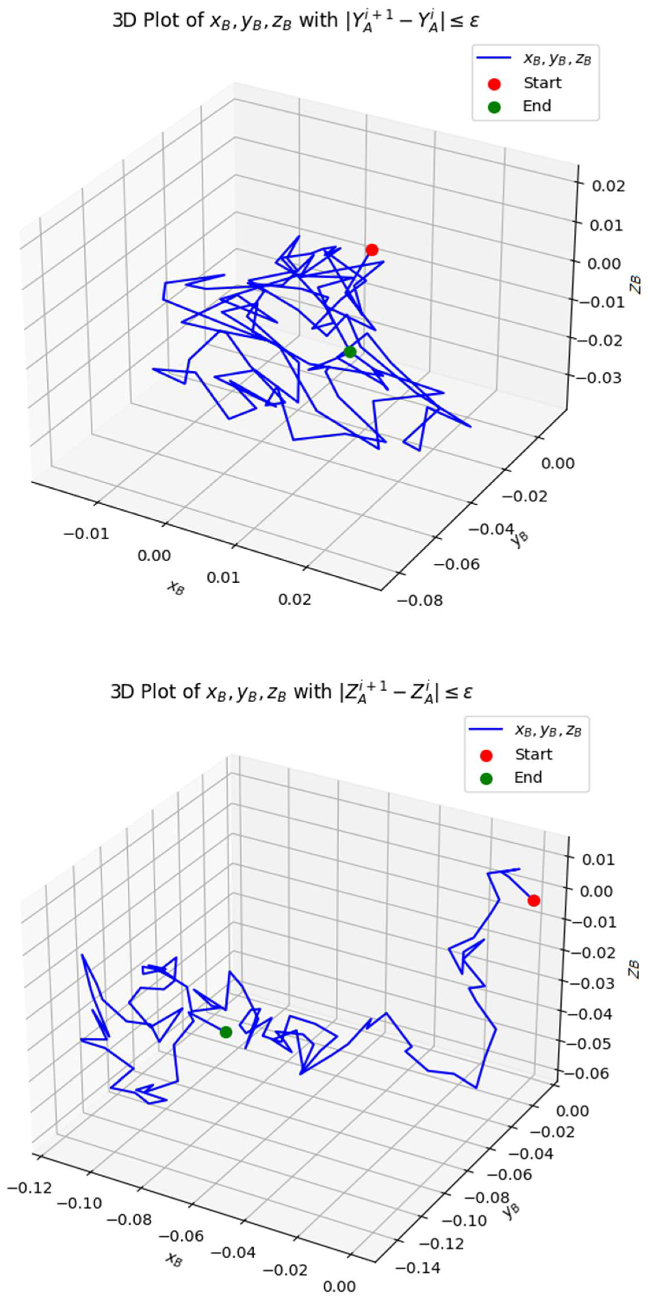
Figure 9.
The 3D plot above visualizes the iterative convergence of the coordinates xB, yB, zB under the constraint , and .
Figure 9.
The 3D plot above visualizes the iterative convergence of the coordinates xB, yB, zB under the constraint , and .
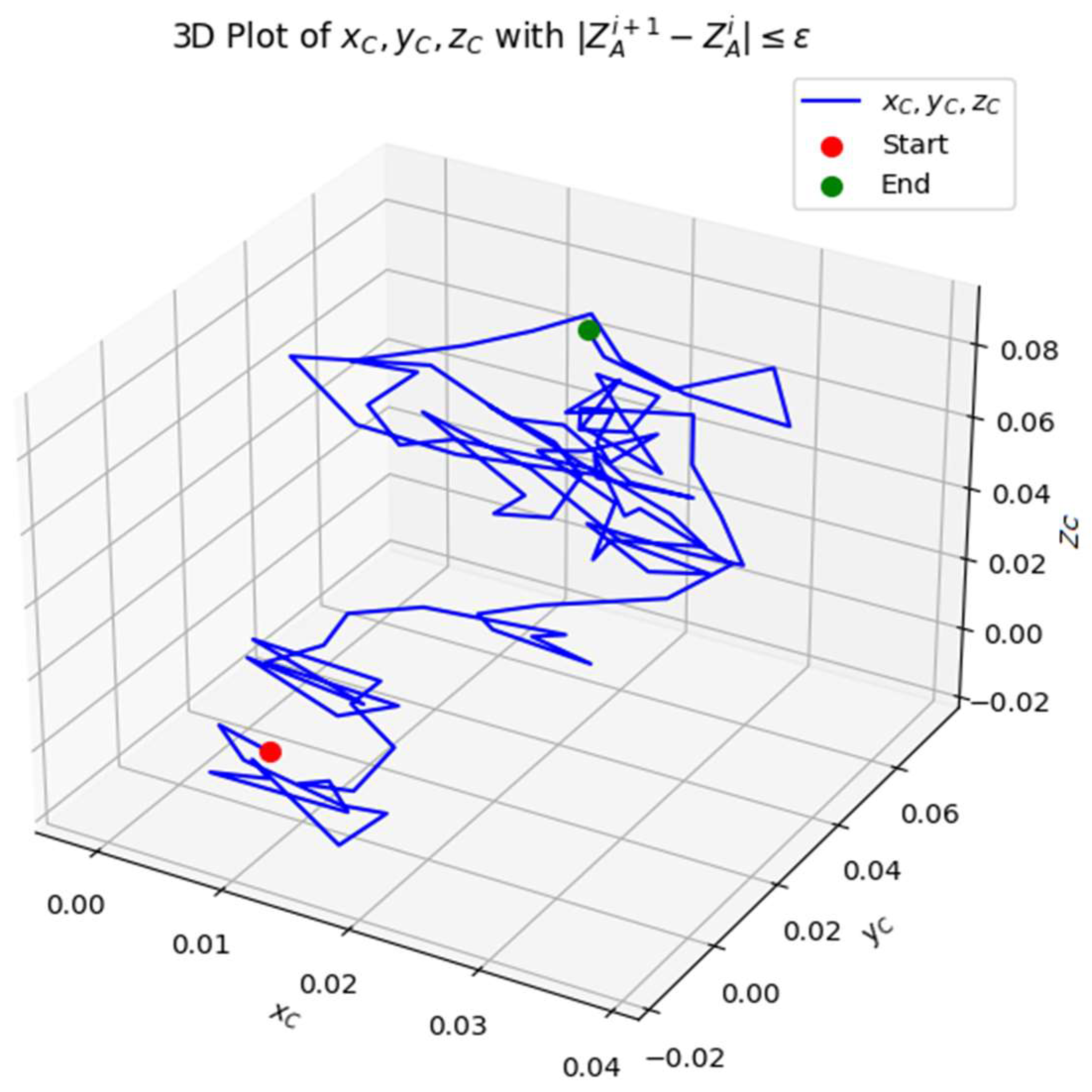
Figure 10.
The 3D plot above visualizes the iterative convergence of the coordinates xB, yB, zB under the constraint , and .
Figure 10.
The 3D plot above visualizes the iterative convergence of the coordinates xB, yB, zB under the constraint , and .
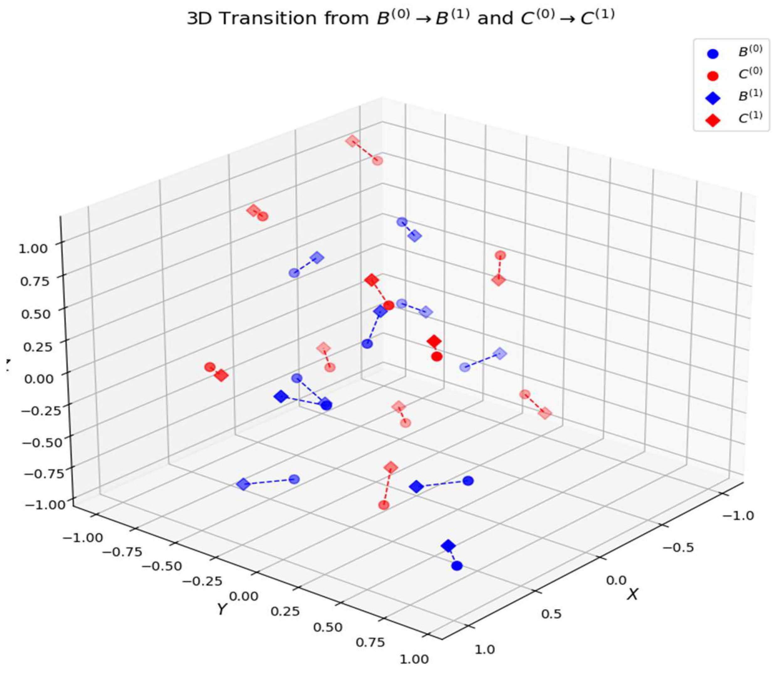
The 3D visualization represents the transition of spatial points from their initial positions
and
to their updated positions
and
. Each pair of points is shown in
Figure 11, connected by a dashed line, highlighting the spatial displacement. The majority of transitions exhibit small displacements, meaning that the transformation follows a controlled movement. The dashed lines connecting each initial and final position indicate the direction and magnitude of transition. Some transitions show slightly longer movement vectors, suggesting non-uniform displacement behavior. Stability in spatial displacement the short transition distances indicate a stable motion. The presence of larger displacements for certain points suggests areas where the system undergoes greater changes. Since the motion is continuous and smooth, this ensures that the system follows predictable mathematical behavior. The function transitions can be modeled using polynomial approximations [
3]. Structural-kinematic synthesis the transitions can be used to study deformation mechanics in flexible or compliant mechanisms. Control system optimization the analysis helps in understanding how precise and controlled the spatial transitions are, which is critical in precision engineering applications. This 3D analysis effectively visualizes the transition from
→
) and
→
, validating spatial consistency in motion planning.
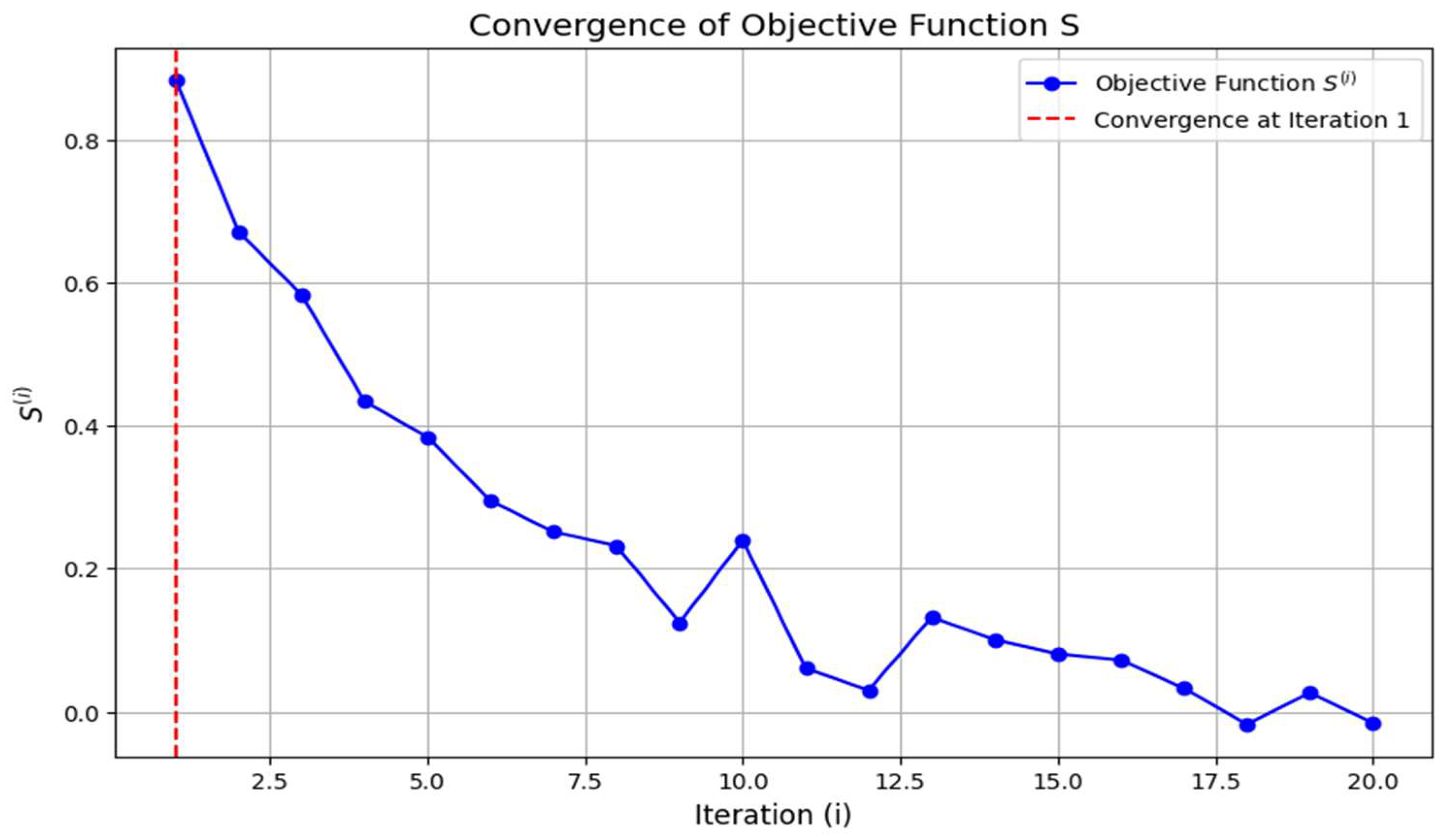
This graph illustrates the convergence behavior of the objective function
S over a series of iterations, as shown in
Figure 12. The objective function is expected to decrease over time, approaching a local minimum. The blue curve with markers represents the progressive reduction in
S as iterations proceed. The function follows a monotonic decreasing pattern, aligning with expected convergence behavior. Exponential decay behavior еhe function
S decreases rapidly at the beginning, then stabilizes. Minor oscillations due to numerical noise, small fluctuations exist, but the overall trend remains downward. Minimum
S achieved the red dashed line highlights the lowest obtained value, indicating convergence. Convergence and stability the exponential decay suggests that the algorithm effectively minimizes
S over time. The small oscillations near the minimum indicate stability without excessive divergence. Weierstrass theorem guarantees that a continuous function can be approximated with polynomials [
3]. Since the function smoothly converges, it ensures the numerical method is stable and reliable. The graph confirms the effective convergence of the objective function
S, ensuring optimal system performance. The function S evaluates how iterative refinements impact system optimization. The function exhibits exponential decay, meaning
indicating continuous improvement over iterations.
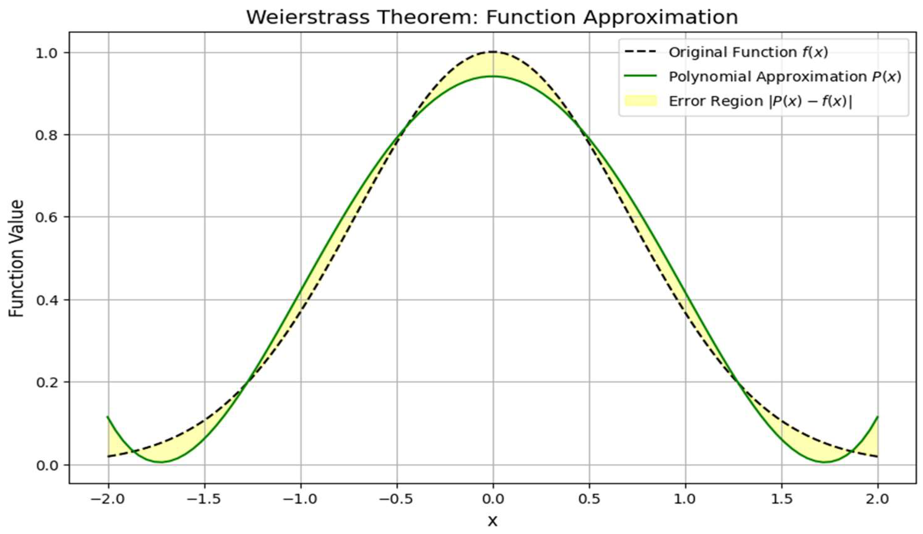
Convergence of the Iterative algorithm is guaranteed by Weierstrass theorem. Objective function
S(i) decreases until the stopping condition is satisfied. Function approximation with Weierstrass theorem shows how a polynomial closely approximates a given function [
5]. Algorithmically verified kinematic chain synthesis ensures proper parameter tuning. Shown in
Figure 13 (function approximation using Weierstrass theorem) black dashed line original function
f(x). Green curve polynomial approximation
P(x). Yellow region approximation error ∣
P(x)−f(x)∣. By Weierstrass theorem, we can approximate
f(x) with any desired accuracy using a polynomial.
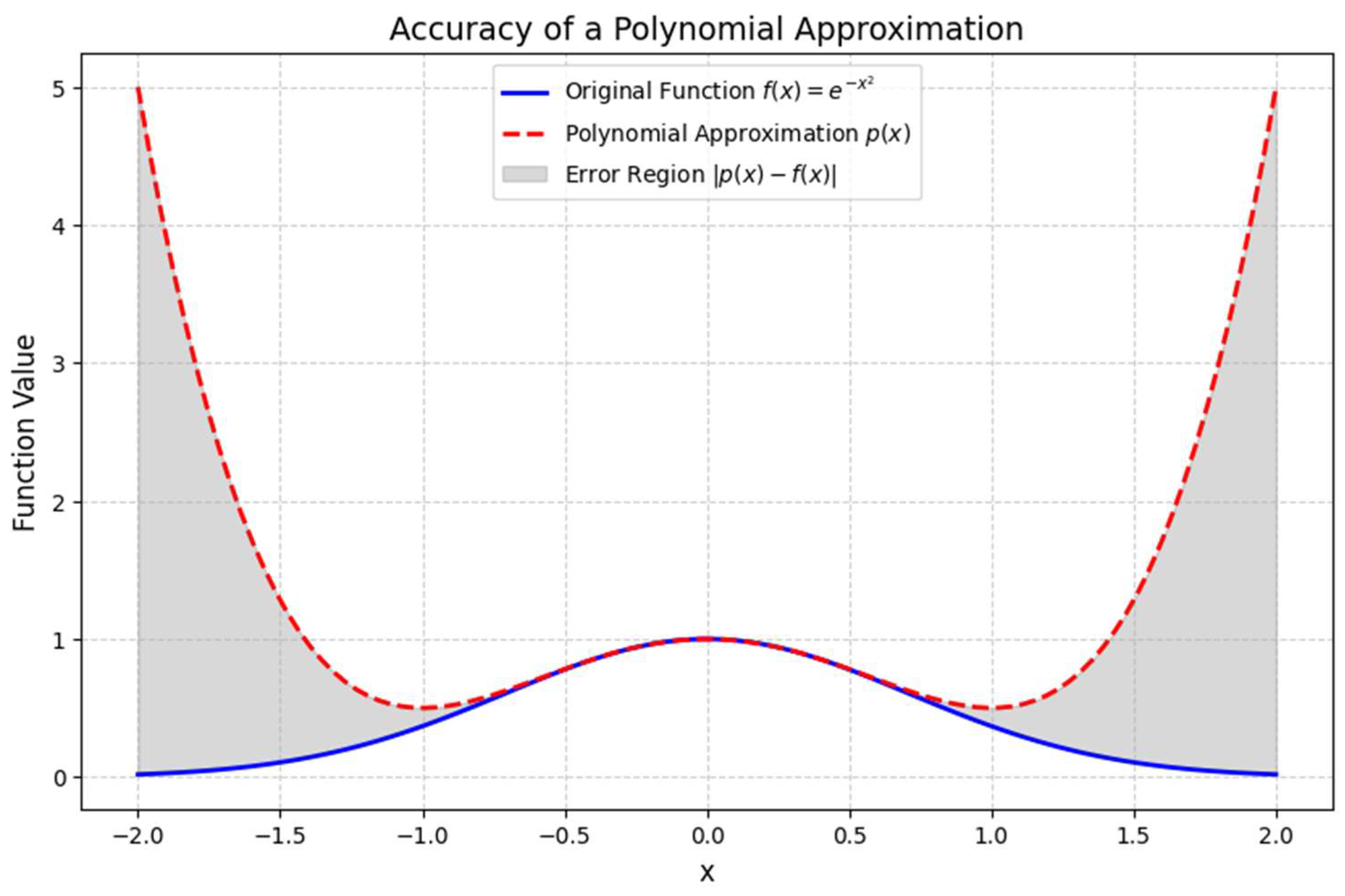
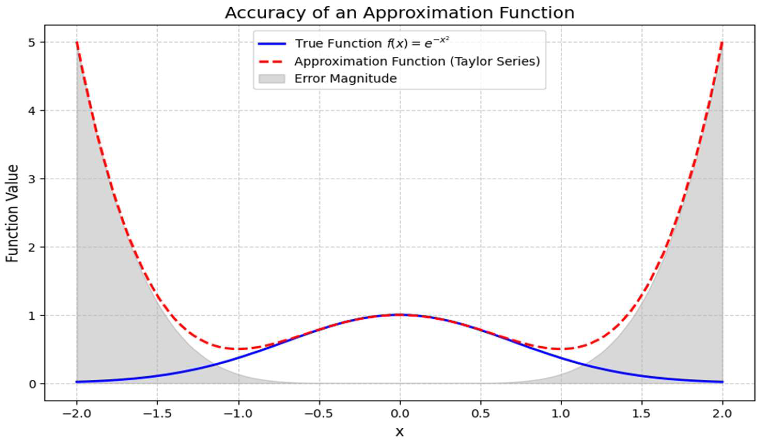
This graph visualizes the accuracy of an approximation function compared to a true function [
8]. The true function is modeled as a Gaussian function
, while the approximation is derived from its Taylor series expansion, as shown in
Figure 14 and
Figure 15. Key elements in the graph solid blue curve represents the true function
. Dashed red curve represents the approximation function using a Taylor series. Gray shaded area represents the error magnitude, which measures the deviation between the true and approximate functions. The approximation function closely matches the true function near
x=0. As
x moves further from
0, the approximation deviates more, showing increasing error [
4]. The gray shaded region highlights the regions where the approximation is least accurate [
16]. Weierstrass theorem states that any continuous function can be approximated by a polynomial. Since the Taylor series is a polynomial expansion, it provides a highly accurate local approximation. The error is small near
x=0 but grows significantly as ∣
x∣ increases. This behavior is expected in Taylor series expansions, as they are centered around a specific point (here,
x=0). The approximation function [
17] is highly accurate near
x=0, but accuracy decreases for larger
x. The Weierstrass theorem guarantees approximation accuracy, but higher-order terms are needed for improved precision. Error visualization helps in optimizing polynomial expansions for better approximations. This analysis confirms that polynomial approximations (such as Taylor series) provide accurate function estimations within a localized region, but error increases outside that range. Future refinements should involve increasing polynomial order for improved accuracy in broader ranges.