
Submitted:
03 September 2025
Posted:
04 September 2025
You are already at the latest version
Abstract
Traditionally, the determination of Denavit–Hartenberg (DH) parameters for serial robotic manipulators is a manual process that depends on manufacturer documentation or user-defined conventions, often leading to inefficiency and ambiguity. This study introduces a universal and systematic methodology for automatically deriving DH parameters directly from a robot’s zero configuration, using only the geometric relationships between consecutive joint axes. The approach was implemented in a MATLAB-based kinematics toolbox capable of computing both the classical and modified DH parameters. In addition to parameter extraction, the toolbox integrates workspace visualization, manipulability and dexterity analysis, and a novel slicing and alpha-shape algorithm for accurate workspace volume computation. Validation was conducted on multiple industrial robots by comparing the extracted parameters with the manufacturer data and the RoboDK models. Benchmark studies confirmed the accuracy of the volume estimation, yielding an absolute percentage error of less than 4%. While the current implementation relies on RoboDK models for verification and requires manual tuning of the alpha-shape parameter, the toolbox provides a reproducible and extensible framework for research, education, and robot design.
Keywords:
DH parameters
; kinematic modeling
; workspace analysis
1. Introduction
Accurate kinematic modeling of robotic manipulators is fundamental for high-precision motion control, offline programming, and overall performance optimization. This accuracy is particularly critical in tasks requiring precise absolute positioning and repeatability, where a strong correspondence between the robot’s virtual model and its real-world actions is essential.
To this end, the Denavit-Hartenberg (DH) convention, first introduced in [1], remains one of the most widely adopted standards for the analytical description of robotic geometry. By systematically assigning coordinate frames to each link, the otherwise complex forward kinematics problem of determining the end-effector pose from joint variables is simplified, making the analysis more tractable for multi-link manipulators. While foundational and widely taught using seminal texts such as [2,3,4], the classical DH framework has some notable limitations. Specifically, in configurations where consecutive joint axes are parallel or nearly parallel, the model can suffer from discontinuities and singularities, leading to numerical instability and unreliable calibration outcomes. Furthermore, the classical convention of placing each joint frame on the axis of the subsequent joint can complicate parameter assignment in certain cases.
To mitigate the limitations of the classical framework, Craig introduced the Modified Denavit-Hartenberg (MDH) convention [5], a formulation notably adopted in influential resources such as Peter Corke’s Robotics Toolbox [6]. Moreover, it has been employed in the widely recognized handbook by Siciliano et al. [7]. By altering the frame assignment, the MDH provides a more robust and often simpler formulation that reduces the numerical sensitivity in problematic axis configurations. This makes it a practical alternative for accurately modeling a broader range of manipulator geometries. Consequently, the MDH convention is often preferred for computational implementations and calibration tasks.
Despite the long-standing use of both conventions, ambiguity in the literature is common, with many publications failing to specify which framework is being applied, leaving readers uncertain regarding the underlying kinematic assumptions. While some studies have sought to alleviate this confusion by clearly delineating the differences between the conventions [8,9], they often stop short of providing algorithmic implementations for systematic parameter derivations.
The need for clear and repeatable methods has motivated several efforts to establish systematic procedures for the direct computation of the DH parameters. For instance, Corke [10] proposed an algebraic walkthrough to derive the parameters for either convention. Faria et al. [11] developed an automatic algorithm using dual vector algebra, though their use of the term "Standard" DH parameters highlights the very ambiguity mentioned earlier. Recently, Sung and Choi [12] introduced an algorithm for modeling MDH parameters using line geometry. While these contributions underscore the ongoing interest in automatic parameter computation, they pave the way for a more universal and user-friendly approach.
Beyond kinematic accuracy, a robot’s workspace is a critical, although often overlooked, metric for performance optimization. The workspace defines the set of reachable poses for the end-effector and is used to identify regions of high accessibility, as highlighted in [13]. Although established numerical methods exist for computing the workspace via random sampling [14], the precise calculation of a manipulator’s total workspace volume remains a challenge. Specifically, the authors identified a gap in the literature regarding methods that can accurately quantify the volume of complex, often non-convex workspaces with potential internal voids that are characteristic of serial manipulators.
Improving robot accuracy through kinematic calibration has been a significant area of research, with methodologies evolving from foundational parametric models to more robust techniques. Early parametric approaches, such as Hayati’s general error mapping method, introduced new parameters to address the modeling challenges of parallel joint axes [15]. Subsequent work was based on geometric principles. Abderrahim and Whittaker introduced a procedure for direct DH parameter identification [16], while others extended this using Dual Vector Algebra to extract DH parameters without requiring base frame calibration [17,18]. Efforts to improve efficiency have led to methods for optimal measurement configuration selection [19] and simplified models showing that calibrating only the home position could yield comparable results [20]. For scenarios lacking prior kinematic information, purely geometric approaches using Singular Value Decomposition and curve fitting have also been developed to determine joint axes [21,22].
Recent research has focused on the challenges of practical implementation and specialized scenarios. To address on-site measurement, Icli et al. [23] developed a novel, low-cost portable measuring device, while Boby and Klimchik [24] proposed a hybrid method effective in constrained workspaces. Further refinements include a two-step method that separates the angle and length parameter calibration [25] and a study addressing the unique challenges of calibrating robots on mobile platforms [26]. Recently, Liu et al. [27] introduced a Variable Projection method that significantly improves convergence and accuracy when no nominal values are available. Across this diverse body of work, the need for an accurate set of baseline DH parameters remains a critical starting point, as the quality of the initial model directly influences the efficiency and success of the entire identification process.
This study addresses the aforementioned challenges and gaps in the literature by presenting a comprehensive solution with the following key contributions.
- 1.
- A universal and systematic methodology for the automatic determination of DH parameters for any serial robot, using only the geometric information of the joint axes in its zero configuration without requiring prior kinematic data.
- 2.
- A novel MATLAB-based kinematics toolbox that implements this methodology, providing user-friendly tools for computing parameters using both classical and modified DH conventions.
- 3.
- Integrated performance analysis features, including the visualization of the robot’s workspace, manipulability, and dexterity, alongside a novel numerical method for accurately computing the total workspace volume.
- 4.
- Seamless integration with RoboDK, enabling the direct import, analysis, and modification of a wide range of industrial and research robot models.
The remainder of this paper is organized as follows: Section 2 details the proposed methodology, beginning with a review of the DH conventions before presenting the universal frame assignment framework, the complete algorithm for parameter determination, and the method for workspace analysis and volume computation. Section 3 presents the validation results, in which the toolbox is applied to several industrial robots to demonstrate its accuracy and robustness. Finally, Section 4 discusses the findings, and Section 5 concludes the paper.
2. Methodology
In the modeling of serial robotic manipulators, the Denavit-Hartenberg (DH) convention is a widely adopted method for systematically describing the geometric relationships between the consecutive links. The original formulation introduced by Denavit and Hartenberg is commonly referred to as the classical DH convention. A modified version, later proposed by John Craig, is known as the Modified DH (MDH) convention. Despite their widespread use, many research publications do not explicitly state which convention is employed, leading to ambiguity in the interpretation and reproducibility of the kinematic models. Therefore, it is essential to clearly distinguish between these two conventions, as even minor differences in parameter definitions can result in significant discrepancies in the derived kinematic equations and their subsequent analysis.
2.1. The Denavit-Hartenberg Conventions
In the classical DH convention, the transformation between consecutive joints and i consists of four basic transformations.
where
The link and joint parameters are denoted as , , and which are referred to as the link twist, link length, link offset, and joint angle, respectively. The joint variable is for a prismatic joint and for the revolute joint.
In the MDH convention, the order of transformations and the numbering of joints change. This leads to the transformation given in (6).
where
A visual comparison between the two methods is presented in Figure 1.
An arbitrary transformation between two frames requires six parameters. Under the following assumptions, this reduces to four parameters:
Assumption 1.
The axis is perpendicular to the axis
Assumption 2.
The axis intersects the axis
We summarize the implication of Assumptions 1–2 below and defer the proof to Appendix A.
Theorem 1
(Four-parameter MDH representation and uniqueness). Let denote the MDH transform given in (6) with rotation and position . Under Assumptions 1–2, is fully parameterized by the four scalars and these parameters are unique.
2.2. Universal Frame Assignment Methodology
To assign frames correctly, a general method is proposed based on the relationship between consecutive joints. This method is applied from joint to i and repeated until the last joint is reached. Some preliminaries are introduced; first, the assignment of the direction vector must be understood, then the assignment of a joint position must be understood, and then the consecutive joint relationships can be explained.
Each joint has a rotational or translational axis. To express a joint in Cartesian space, its direction and position must be defined with respect to a common coordinate frame. This coordinate frame is the reference for each joint and is defined as the world frame, which is denoted by the symbol .
Definition 1
(World Frame). The world frame, denoted by the symbol , is a common coordinate frame that serves as a universal reference for all objects in the workspace, including the position and direction of each joint.
The world frame is arbitrary and can be selected in any orientation. Throughout this study, the convention is as follows: the z-axis points up, the x-axis points right, and the y-axis is the cross product of the z and x axes.
Definition 2
(Direction vector of a joint). Let be a free unit vector, it is the direction vector of joint i if it is parallel to joint axis i.
The direction vector can be in either direction of the joint axis. The chosen direction determines the positive rotation or translation direction of the joint; however, it does not affect the resulting kinematic structure.
Definition 3
(Position of a joint). Let be a fixed vector with its origin at the world frame. This vector is the joint position if it lies on any point of the joint axis.
The joint position can be an arbitrary point on a joint axis because the computation of the consequent frame assignment and DH parameters will depend on the relationship between consecutive joint axes, and not the joint positions. The joint position can easily be inferred by looking at a manufacturer’s datasheet of a robot, as the translational or rotational axes exact positions are always given.
From here on in this paper, whenever a reference frame is not specifically written in vector notation, it is always w.r.t the world frame, for example, . Finally, a joint’s axis can be defined as a parametric function of the form
where t is a parametric variable and is a vector with its origin on the world frame, and its tip at a point on the joint axis. Note that when the parametric variable , the vector becomes the joint position.
An example is provided to obtain a better understanding of the definitions. Two joints are defined and shown in Figure 2, with their corresponding parametric functions as
where s and t are parametric variables, and are the positions of joint 1 and 2 respectively, and and are the direction vectors of joint 1 and 2 respectively.
The direction vector of a joint can be defined in several ways, the most intuitive of which is to define it in terms of the world frame axes. In Figure 2, the unit vector is aligned with the z axis of the world frame, thus it can be written as . The unit vector is in the x-z plane of the world frame and has an angle of 45 °w.r.t the x-axis. Thus it has equal components in both x and z directions, which can be written as .
Another method to define the direction vector of a joint is to express it with a series of rotations. For example, the vector can be expressed as the vector rotated along the axis by or as rotated along the by . This is shown in the following equation
Throughout this work, the unit vector approach will be used to define the direction vector of a joint, since the authors believe it is more intuitive. The joint position and direction vectors will now be used to compute the DH frames and DH parameters; however, before moving on, the relationships between consecutive joint axes must be explained.
Before placing the frames, the relationship between consecutive frames defined a framework for how the origin and x-axis should be placed. In 3D space, subsequent joint axes can be in four states with each other: skew, intersecting, parallel, or collinear.
To check how consecutive joint axes are related to each other, some cases are introduced.
Characterization 1
(Geometric Conditions Between Joint Axes). Let and be the direction vectors of joints i and , respectively, and let
denotes the position vector from joint i to joint , expressed in the world frame.
The following three geometric conditions were defined:
-
Condition C1 (Axis Alignment):This condition holds when the joint axes are parallel or collinear.
-
Condition C2 (Coplanarity):This condition holds true if the joint axes lie in the same plane.
-
Condition C3 (Axis Coincidence):This condition holds if the origin of joint lies along the axis of joint i.
These conditions are used throughout this study to categorize the spatial relationships between consecutive joint axes.
Now that the conditions are characterized, we can determine the state of the consecutive joints by combining these conditions. The results are presented in Table 1.
Now, the frame placement framework based on the geometric relationship between consecutive joint axes is introduced. The process of defining the MDH frames for the intersecting joint axes is illustrated in Figure 3.
After the position and direction vectors of joints i and are determined, the origin must be placed at the intersection point. This intersection point is labeled and represents the origin of the MDH frame. Then, the already determined direction vector is placed with its origin at , fixing the vector in 3D space. The unit vector is placed normal to the plane defined by the basis vectors and in either direction. Although not used in computations, the axis is defined as To mathematically write this process, we define the parametric function of the joint axes as
Where s and t are parametric variables. Substracting (16) from (15) yields the following matrix equality
Since the equality is overdetermined, a pseudo inverse can be taken that minimizes the least square error as follows
Now the parametric variables s and t are found, which can be used in either (15) or (16) to find the origin of the frame as
Since the joint axes are coplanar, the x axis is placed along the normal to this plane either positively or negatively, which fully defines the MDH frame of joint i.
The next geometric relationship is the skew axes, which are defined as axes that do not intersect and are not parallel. The process of assigning a frame to joint i is shown in Figure 4.
When the position and direction vectors of joints i and are determined, a common orthogonal line between these axes is drawn, indicated by the brown line segment in the second part of Figure 4. The origin is placed at the intersection of this common orthogonal line segment and joint axis i. The origin of the axis is fixed to and the axis is placed along the common orthogonal line.
The parametric functions of the joint axes are defined similarly to (15) and (16). The vector connecting these axes is defined as the multivariable function
To find the common orthogonal line segment, which is also the unique shortest line segment for skew axes, the minimum of (21) must be found.
Writing (21) in (22) yields the following equation
The partial derivates w.r.t s and t are written and set equal to 0 to find the parametric variables that minimize .
This yields the following matrix equation to find the parametric variables s and t.
The common orthogonal line segment is now known and the frame origin can now be obtained by substituting s into joint axis as follows
The x axis is placed along the common orthogonal line segment, which was defined as , therefore it can be written as follows
Next, the parallel axes were considered. A distinction between the parallel and collinear axes is made because both require different procedures to assign frames. The process for the parallel frames is shown in Figure 5.
The process for parallel axes is similar to that of skew axes, however, the common orthogonal line segment is non unique, leading to an infinite amount of common line segments. Therefore, one must be chosen to minimize the number of additional parameters. This is commonly chosen as the position of joint i. The next steps are similar to those of the skew axes, the vector’s origin is fixed at and the vector is placed along the common orthogonal.
The parametric functions are defined similarly to the previous steps and (15) and (16). Since the origin of the frame is chosen at the position of joint i as
the parameter s is zero and . This makes the line segment equation as follows
Since the line segment must be orthogonal to the direction vector of joint , the following equality can be written
From this equality, t can be computed by substituting (33) in (34) and is obtained as follows
This yields the following expression for the x axis
Collinear axes are the final geometric relationships and are the most obscure. These axes are defined as being aligned and coincident. The process of assigning the frame to joint i is illustrated in Figure 6.
Since the axes coincide, the origin is placed on an arbitrary point on the axes. As in the parallel axis case, the position of joint i is preferred.
The z-axis was placed along the joint axis. The axis is placed anywhere on the plane normal to the axis, which makes it impossible to determine exactly. Therefore, for collinear axes, a secondary framework must be used for logical assignment.
The framework for assigning the axis in collinear frames is divided into two parts: joint i being the first joint in the robot or joint i being any joint other than joint 1 in the robot. In the former case, is checked to determine whether it is perpendicular to any of the main axes of the world frame. If it is perpendicular to any, the is chosen as that axis. If it is not perpendicular to any of the world frame axes, the axis with the smallest angle to is chosen as the axis. If multiple
In the latter case, namely when the iteration is at a joint other than the first, the axis is chosen in the same direction as the previous axis .
The MDH frames for joints 1 through N-1 have been established, but the base frame and frame of the last joint remain undefined. To address this issue, two assumptions were introduced. The first assumption is that the base frame coincides with the MDH frame of joint 1 such that the origins and x- and z-axes are identical. The second assumption is that the final MDH frame N coincides with the position of the last joint while sharing the same x-axis orientation as the MDH frame of joint N-1.
Now that the MDH frames are obtained, the MDH parameters can be extracted using the following equations:
2.3. Algorithm for Automatic DH Parameter Determination
The first step in determining the MDH parameters is to establish a geometric relationship between consecutive joint axes. Algorithm 1 performs this classification by analyzing the orientation vectors of each pair of consecutive joints and their relative displacements. Conditions C1, C2, and C3 are used to distinguish whether the axes are intersecting, skew, parallel, or collinear. This classification is crucial because it dictates how the coordinate frames are assigned in the next stage. Without correctly identifying these relationships, the subsequent frame placements and parameter extractions would be inconsistent and error-prone.
| Algorithm 1 Axis Relation Classification |
|
Once the axis relationships are identified, Algorithm 2 systematically assigns frames according to the geometric state of each joint pair. For example, when two axes intersect, the origin of the frame is placed at their intersection, and the x-axis is oriented normal to the plane defined by the two z-axes. For the skew axes, the algorithm determines the shortest common orthogonal line segment and uses it to define both the frame origin and x-axis direction. In the case of parallel axes, the origin is fixed at the position of the preceding joint, whereas for collinear axes, additional rules ensure consistency across joints. Thus, this algorithm provides a universal and repeatable method for assigning MDH frames without relying on ad hoc or manual decisions, ensuring that the computed parameters remain valid for arbitrary serial robot geometries.
| Algorithm 2 Find MDH-Related Frames from Axis Relations |
|
After the frames have been assigned, Algorithm 3 calculates the MDH parameters directly from the frame origin, z axes, and x axes computed using Algorithm 2. Using simple vector operations and the definitions of the twist angle (), link length (a), link offset (d), and joint angle (), the algorithm iteratively computes the full MDH table. Each parameter was obtained by projecting the difference between the consecutive frame origins onto the appropriate axis or by evaluating the relative orientation between the frame axes. Importantly, this algorithm does not require any prior knowledge of the robot geometry beyond the joint axis definitions, making it generalizable to any serial manipulator. The computed parameters can then be directly used for forward kinematics and further analyses, such as workspace computation.
| Algorithm 3 Compute MDH Table from Frame Triplets |
|
Because the MDH parameters are computed, forward kinematics can be performed using (6) to determine the transformations from to .
2.4. Workspace Analysis and Volume Computation
To provide a comprehensive kinematic analysis, the toolbox integrates functionalities for evaluating a robot’s workspace, including the computation of performance indices and estimation of its total volume. The workspace is defined as the set of all reachable end-effector positions.
The analysis begins with the generation of a point-cloud representation of the workspace using the Monte Carlo method. This approach, implemented in C++, involves generating a large number of random joint configurations using a pseudorandom generator std::mt19937. For each configuration, the joint angles were sampled from a uniform distribution within their predefined limits. The forward kinematics based on the MDH are then computed to determine the resulting Cartesian position of the end-effector. This process yields a dense point cloud that effectively represents the robot’s reachable volume.
At each point in this cloud, the robot’s geometric Jacobian matrix is calculated to evaluate the local performance characteristics. The jacobian is computed column by column, where each column can be found using
where the vector is the direction vector of joint i w.r.t the base frame and can be found using the forward kinematics as the third column of the transformation matrix , the vector is the position of the end effector if it is defined. If not defined, this is taken as the position of the last frame . The vector is the origin of frame i w.r.t the base frame, and is an operator defined as follows
Using the defined Jacobian, the toolbox computes two key metrics:
-
The manipulability index (), based on Yoshikawa’s work, quantifies the robot’s ability to move its end-effector in any direction. It is calculated as the square root of the determinant of .A higher value indicates greater ease of motion, whereas a value of zero corresponds to a singularity.
-
The dexterity index, which measures the isotropy of the manipulator’s motion, is calculated as the ratio of the minimum singular value () to the maximum singular value () of the Jacobian matrix. This is equivalent to the inverse of the Jacobian condition number.A value close to 1 indicates that the end effector can move with equal ease in all directions, whereas a value close to 0 suggests that the robot is near a singularity.
These indices were visualized as a color map overlaid on the workspace point cloud, offering an intuitive understanding of the robot’s performance across different regions.
The novel contribution of this study is a numerical method for computing the workspace volume. Because the workspace of a serial manipulator is often non-convex with potential voids, a simple convex hull would yield an inaccurate overestimation. To address this, our method employs a slicing technique combined with alpha-shapes. The procedure was as follows:
- 1.
- Slicing: The 3D workspace point cloud is partitioned into a series of thin, parallel slices of a uniform thickness, , along the z-axis.
- 2.
- 2D Projection and Boundary Finding: For each slice, the points contained within it are projected onto the x-y plane. An alpha shape is then generated from the 2D point set. The alpha shape algorithm creates a tight, potentially non-convex boundary that accurately envelops the points, effectively capturing the shape of a specific cross-section, including any internal holes. The alphaRadius is a critical parameter that controls the tightness of the boundary.
- 3.
- Area and Volume Summation: The area () of the alpha shape for each slice i is calculated. The volume of the slice () is then approximated as . The total workspace volume is estimated by summing the volumes of all slices as follows:
This method provides an accurate estimation of the true workspace volume, accommodating the complex geometries characteristic of multi-link manipulators.
Using the MDH parameters obtained from Algorithm 3, the joint types for each joint and an optional joint angle or displacement parameter , forward kinematics can be performed, as presented in Algorithm 4.
| Algorithm 4 ForwardKinematics (Modified DH, cumulative) |
|
The input are the angles at the zero position. Using the obtained forward kinematics algorithm, the Jacobian can be obtained using Algorithm 5.
| Algorithm 5 Jacobian computation |
|
The sampling of the workspace is performed as defined in Algorithm 6 where the input S represents the number of sampled joint configurations.
| Algorithm 6 Workspace Sampling with MDH Kinematics |
|
The computation time for Algorithm 6 greatly depends on the number of sampled joint configurations S and the number of joints in the robot N. For the fastest computation time, Algorithms 4–6 were implemented in C++ and compiled with MinGW-w64 into MEX files for use in MATLAB. Using the obtained end-effector positions and performance indices for each joint configuration, a visualization of the workspace can be obtained. Slices can also be viewed along the xy, yz, and xz planes by indexing the positions from the algorithm at an interval of the axis normal to the sliced plane.
The algorithm for computing the workspace volume is presented in Algorithm 7.
| Algorithm 7 Workspace Volume Computation |
|
The proposed algorithms were directly implemented in the toolbox for workspace analysis and workspace volume computation.
2.5. Linking the toolbox with RoboDK
RoboDK is a widely used offline robotic programming and simulation software that provides tools for path planning, calibration, and robot programming across a broad range of industrial applications. One of its main advantages is the extensive built-in library of commercial robot models, which allows users to readily import manipulators from multiple manufacturers without requiring detailed kinematic specifications of the manipulators. This feature makes RoboDK an effective source for benchmarking and validating kinematic algorithms. Moreover, the availability of the MATLAB API enables seamless integration between RoboDK and external computational toolboxes, facilitating direct data exchange and joint analyses. In the context of the present work, this integration was leveraged to import robot models into the developed MATLAB toolbox, ensuring reproducibility, reducing manual input, and allowing parameter extraction and workspace analysis to be carried out consistently across different robotic platforms.
To import a robot from the RoboDK library, the user first opens the RoboDK environment and loads the desired robot model into their workspace. The joint configurations of the selected robot were then accessed via the RoboDK MATLAB API, which enabled direct programmatic interaction with the simulation environment. These joint poses were extracted and used within the developed toolbox to define the corresponding joint positions and direction vectors, thereby ensuring consistency between the RoboDK model and MATLAB-based kinematic representation. Importantly, all these steps can be performed using the free version of RoboDK. The licensed version additionally provides access to both classical and MDH parameters of the robot, which were used in this study to validate the results of the toolbox computations.
3. Results
The proposed methodology was verified using a library available in RoboDK. From this library, four different types of industrial robots were selected to ensure that all geometric conditions existed. The results were obtained for the frame placement and DH parameters, workspace analysis, and volume computation for each robot. Furthermore, to verify the results of the frame placement and DH parameters, the available manufacturer data were used. Where not available, the parameters in RoboDK were used for comparison. Finally, for the workspace volume, because manufacturer data were not available and no sources were found by the authors, analytically computable robots were created as a reference to compare the proposed methodology.
3.1. Overview of the Kinematics Toolbox
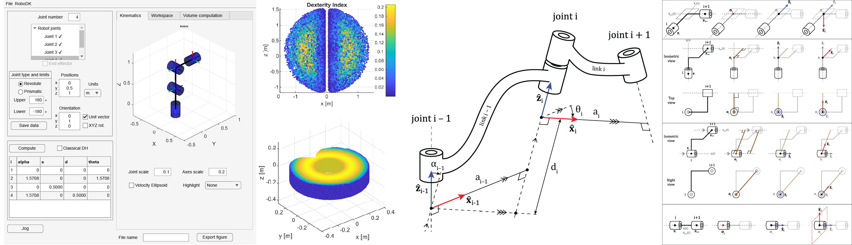
An overview of the toolbox is provided below. A detailed description of how to use the toolbox is available on the GitHub page [28]. The toolbox consists of three main sections: the joint definition, DH parameter computation, and visualization sections. The visualization section consists of three main tabs: the Kinematics tab, the Workspace tab, and the Volume Computation tab. The toolbox with the three different tabs is presented in Figure 7.
The top-left section of the interface is designated for the joint definition, where the user specifies the number of joints. Once defined, a joint can be selected from the tree selection panel, and its parameters, including the joint type, limits, position, and direction vector, are entered. After completing the input, the Save Data button stores the parameters of the selected joint, which are then visualized in the Kinematics tab of the GUI. Following the definition of all joints, the user proceeds to the DH parameter computation section at the bottom-left, where pressing the Compute button generates the DH parameters. By default, the MDH convention is displayed, but the user can toggle between the MDH and classical DH using the adjacent checkbox.
In the Kinematics tab, presented in Figure 7(a), the robot structure can be visualized with options to adjust the scales of the joints and axes. Once the DH parameters are computed, individual joints can be highlighted to examine the frame placement. An additional feature, the Jog button, opens a separate window that allows the interactive jogging of the defined robot within the plot environment.
The Workspace window in Figure 7(b) provides tools for specifying the number of randomly generated samples and slicing the workspace along the xy, yz, and xz planes. The slice positions can be adjusted using a slider, enabling the examination of different cross-sections. The user can also toggle between the manipulability and dexterity indices. A slice thickness field is available to adjust the thickness of the visualized slice, which improves the visualization quality and enables accurate volume computation.
The Workspace Computation tab includes the functionality for alpha-shape parameter adjustment, as shown in Figure 7(c). The left plot displays the center slice, while the right plot shows a movable slice controlled by a position slider, allowing the user to observe the alpha shapes across different sections. Once the desired alpha shapes are achieved, the Compute Volume button calculates and outputs the workspace volume.
Finally, the interface includes an Export Figure option in the bottom-right corner, which enables the user to export the currently displayed figure from any tab using a specified file name.
The developed toolbox is made available as executable MATLAB P-code files, allowing researchers and educators to use the software while preventing the direct modification of the source code. The toolbox is distributed under the CC BY-NC-ND 4.0 license and is accessible via the project’s GitHub repository [28]. This ensures the reproducibility of the results while reserving future development opportunities for the authors.
3.2. Frame Placement and DH Parameters
The ABB IRB 1100-4/0.58, which will be referred to as IRB 1100 from here on for simplicity, contains intersecting, parallel, skew, intersecting, and intersecting joint axes. The robot is saved in the ABB-IRB1100.mat file for verification. The results of the frame placement are presented in Figure 8. The extraction of the MDH parameters was performed using the proposed methodology, and the results are presented in Table 2.
These results show that the toolbox can successfully compute the MDH parameters. The differences between the RoboDK reference and toolbox results were due to the arbitrary direction of the z-axis. This can be inferred by looking at the last row, where the toolbox took the z-axis in the negative direction of the RoboDK result. Furthermore, the positive or negative direction of the x-axis is arbitrary, as can be seen in rows 5 and 6, where a rotation only switches the direction of the x-axis. Although the computed MDH parameters are correct, their validity is questionable because both the baseline and resulting MDH parameters, which are computed through the joint poses, are derived from RoboDK, creating a dependency on a single platform. This limitation is addressed in the subsequent robot results.
To address the previously noted limitation of relying on a single platform for comparing the results, the UR10e robot was selected. For this robot, the manufacturer provided data for the classical DH parameters, enabling verification by comparing the parameters obtained from RoboDK with the independently available manufacturer specifications. The manufacturer classical, computed classical, and MDH parameters are presented in Table 3. Manufacturer data were obtained from UR support articles [29].
The MDH frame placement results for the UR10e robot are shown in Figure 9.
3.3. Workspace Analysis
Workspace analysis for the ABB IRB 1100-4/0.58 was performed by sampling 1,000,000 random joint configurations within the joint limits and performing forward kinematics to obtain the end-effector pose. The Yoshikawa manipulability index over the full workspace is shown in Figure 10.
Because the toolbox also allows the dexterity analysis to be viewed, the EPSON T3-401S was sampled at 500,000 random joint configurations within the joint limits, and the end effector’s position was obtained by performing forward kinematics. The dexterity index over the full workspace is shown in Figure 11.
3.4. Volume Computation
To verify the results of the volume computation, some benchmark robots were introduced, whose volumes were easily analytically computable. First, a robot with a spherical workspace and an empty sphere inside is introduced. Second, a robot that draws a slot shape in a plane and can translate along the axis normal to that plane is introduced. Finally, the area of the EPSON T3-401S robot along its slice was computed using CAD software, after which it was multiplied by the distance the prismatic joint could move to obtain its volume. The MDH parameters of the defined robots are listed in Table 4. The joint limits for all revolute joints are and for prismatic joints, .
To analytically obtain the area of the slot robot, the radius r was set to 2 m and the length L to 6 m. The displacement of the prismatic joint h is 2 m so the volume can be computed as
By sampling 1 million joint configurations using a slice thickness of m and an alpha value of ∞ (which results in a convex hull), the workspace volume was computed by the proposed algorithm as . This yielded a percentage error of .
Next, a spherical robot is considered. This robot has an outer () and inner () radius of 3 m and 1 m, respectively. Thus it’s volume can be easily calculated using
By sampling 1 million joint configurations, using a slice thickness of m and an alpha value of , the workspace volume was computed by the toolbox as , which resulted in a percentage error of .
Finally, the EPSON T3-401S was considered. The area drawn by this robot is obtained by drawing a slice of the robot along the prismatic joint using Fusion and is found to be . Hence, the volume can be computed by multiplying the area by the maximum displacement of the prismatic joint, which is m. The volume is thus approximated as . The toolbox was configured to sample 500,000 joint configurations, with a slice thickness of m and an alpha value of . Running the volume computation algorithm a volume of is obtained, which has a error compared to the approximated value.
Because the benchmark robots obtained percentage errors of less than 4%, it is assumed that when the parameters are tuned correctly in the toolbox, a workspace volume with a low error is computed. Tuning these parameters requires manually examining how the alpha shape algorithm performs in computing the areas of a slice. This is easily performed using the visual slicing available in the toolbox.
The combined results of the volume computation algorithm for the benchmark and all other robots, with the corresponding parameters, are listed in Table 5.
4. Discussion
The proposed methodology and toolbox enable the automatic determination of Denavit–Hartenberg parameters directly from the zero configuration of any serial manipulator. Validation across different robot types, including industrial manipulators (ABB IRB 1100, UR10e, KUKA iiwa 7, EPSON T3-401S) and custom benchmark models, demonstrated that the approach can reliably compute both the classical and MDH parameters without manual intervention. The consistency of the computed parameters with the manufacturer data for the UR10e confirmed the correctness of the algorithm, whereas the results obtained for the ABB IRB 1100 and Epson T3-401S highlighted the general applicability of the toolbox to robots with diverse geometric configurations.
Beyond parameter extraction, the integration of the workspace and performance analysis provides additional insight into manipulator capabilities. The manipulability and dexterity indices capture regions of high and low accessibility within the workspace, which can support design evaluation and task planning. The proposed slicing-and-alpha-shape volume estimation method further extends the analysis by quantifying the workspace volume with errors below 4% for analytically verifiable benchmarks. This indicates that the approach can achieve sufficient accuracy for comparative studies of robot reachability, although parameter tuning (slice thickness, alpha radius) remains necessary for optimal performance.
Despite these strengths, several limitations exist. First, the current validation relied in part on RoboDK models, which introduced a dependency on a single simulation environment. Although this allowed for broad testing, independent experimental validation using measurement-based data would further strengthen the conclusions. Second, the accuracy of the workspace volume estimation is sensitive to the choice of alpha shape parameters, which currently require manual adjustment by the user. Automating this selection process would enhance robustness and reproducibility. Third, the methodology assumes accurate knowledge of the joint axes and positions; in practice, extracting this information from CAD models or sensor data may introduce additional sources of uncertainty that have not yet been addressed by the toolbox.
Compared to existing approaches for DH parameter identification, which often require manual frame assignment or specialized algebraic formalisms, the proposed methodology offers a more universal and user-accessible solution. By embedding the algorithms within a MATLAB graphical interface, the toolbox reduces the barrier to adoption in both research and education. This distinguishes it from earlier automatic algorithms, which remain primarily theoretical or require expert-level implementation efforts.
Several promising directions for future research have been identified. First, extending the proposed methodology to parallel and hybrid mechanisms would significantly broaden its applicability to modern robotic systems. Second, automating the selection of alpha shape parameters would reduce user intervention and improve the robustness of the workspace volume estimation. Third, integrating experimental data acquisition methods, such as vision- or sensor-based identification of joint axes, would enable the direct application of the framework to physical robots rather than being limited to simulation environments. In addition, implementing forward dynamics using iterative Newton–Euler algorithms allows the estimation of joint forces and torques, thereby facilitating dynamic analysis. Finally, coupling automatic kinematic model generation with dynamic model derivation would open pathways toward unified model-based control and simulation within the same toolbox.
In summary, the discussion highlights that although the proposed approach provides a reproducible and systematic solution for DH parameter extraction and workspace analysis, future developments are necessary to fully address experimental robustness, automation of parameter tuning, and generalization to broader classes of robotic systems.
5. Conclusions
This study presents a universal methodology and MATLAB-based toolbox for the automatic determination of Denavit–Hartenberg parameters of serial manipulators. By classifying the joint axis relationships and systematically assigning frames, the toolbox computes both classical and MDH parameters without manual intervention. Integrated features for workspace analysis, manipulability and dexterity evaluation, and volume estimation extend their utility beyond parameter extraction. Validation on industrial and benchmark robots confirmed the accuracy of the approach, with workspace volume errors below 4%. The proposed framework reduces the reliance on manufacturer data, increases reproducibility, and provides an accessible platform for research, education, and design. Future extensions will address automated parameter tuning, experimental validation, and the inclusion of parallel and hybrid mechanisms in the model.
Author Contributions
Conceptualization, H.K. and Z.B.; methodology, H.K. and Z.B.; software, H.K.; validation, H.K. and Z.B.; formal analysis, Z.B.; investigation, Z.B.; resources, H.K.; data curation, Z.B.; writing—original draft preparation, H.K.; writing—review and editing, Z.B.; visualization, H.K.; supervision, Z.B.; project administration, Z.B. All authors have read and agreed to the published version of the manuscript.
Funding
This research received no external funding.
Conflicts of Interest
The authors declare no conflicts of interest.
Appendix A Proof of Theorem 1
Assumption (2) states that the and Thus the transformation between the origins of joint and i can be written as a linear combination in terms of the axis the as follows
This demonstrates that, under the given assumption, two parameters are sufficient because (A9) is in the form of (6).
References
- Denavit, J.; Hartenberg, R.S. A Kinematic Notation for Lower-Pair Mechanisms Based on Matrices. Journal of Applied Mechanics 1955, 22, 215–221. [CrossRef]
- Paul, R.P. Robot manipulators: mathematics, programming, and control, 9. printing ed.; The MIT Press series in artificial intelligence, MIT Pr: Cambridge, Mass., 1992.
- Spong, M.W.; Vidyasagar, M. Robot dynamics and control; John Wiley & Sons, 2004.
- Siciliano, B., Ed. Robotics: modelling, planning and control; Advanced textbooks in control and signal processing, Springer: London, 2009.
- Craig, J.J. Introduction to robotics: mechanics and control, fourth edition ed.; Pearson: NY NY, 2018.
- Corke, P.I. Robotics, vision and control: fundamental algorithms in MATLAB, 2nd revised, extended and updated ed ed.; Number 118 in Springer tracts in advanced robotics, Springer: Cham, 2017.
- Siciliano, B. Springer Handbook of Robotics, 2nd ed ed.; Springer Handbooks Ser, Springer International Publishing AG: Cham, 2016.
- A Chennakesava Reddy. DIFFERENCE BETWEEN DENAVIT - HARTENBERG (D-H) CLASSICAL AND MODIFIED CONVENTIONS FOR FORWARD KINEMATICS OF ROBOTS WITH CASE STUDY. International Conference on Advanced Materials and manufacturing 2014. Publisher: Unpublished, . [CrossRef]
- Wang, H.; Qi, H.; Xu, M.; Tang, Y.; Yao, J.; Yan, X.; Li, M. Research on the Relationship between Classic Denavit-Hartenberg and Modified Denavit-Hartenberg. In Proceedings of the 2014 Seventh International Symposium on Computational Intelligence and Design, Hangzhou, China, December 2014; pp. 26–29. [CrossRef]
- Corke, P. A Simple and Systematic Approach to Assigning Denavit–Hartenberg Parameters. IEEE Transactions on Robotics 2007, 23, 590–594. [CrossRef]
- Faria, C.; Vilaca, J.L.; Monteiro, S.; Erlhagen, W.; Bicho, E. Automatic Denavit-Hartenberg Parameter Identification for Serial Manipulators. In Proceedings of the IECON 2019 - 45th Annual Conference of the IEEE Industrial Electronics Society, Lisbon, Portugal, October 2019; pp. 610–617. [CrossRef]
- Sung, M.; Choi, Y. Algorithmic Modified Denavit–Hartenberg Modeling for Robotic Manipulators Using Line Geometry. Applied Sciences 2025, 15, 4999. [CrossRef]
- Zacharias, F.; Borst, C.; Hirzinger, G. Capturing robot workspace structure: representing robot capabilities. In Proceedings of the 2007 IEEE/RSJ International Conference on Intelligent Robots and Systems, San Diego, CA, USA, October 2007; pp. 3229–3236. [CrossRef]
- Cao, Y.; Lu, K.; Li, X.; Zang, Y. Accurate Numerical Methods for Computing 2D and 3D Robot Workspace. International Journal of Advanced Robotic Systems 2011, 8, 76. [CrossRef]
- Hayati, S. Robot arm geometric link parameter estimation. In Proceedings of the The 22nd IEEE Conference on Decision and Control. IEEE, 1983, pp. 1477–1483. [CrossRef]
- Abderrahim, M.; Whittaker, A. Kinematic model identification of industrial manipulators. Robotics and Computer-Integrated Manufacturing 2000, 16, 1–8. [CrossRef]
- Chittawadigi, R.G. Geometric Model Identification of a serial Robot. In Proceedings of the IFToMM International Symposium on Robotics and Mechatronics. Research Publishing Services, 2013, pp. 730–738. [CrossRef]
- Hayat, A.A.; Chittawadigi, R.G.; Udai, A.D.; Saha, S.K. Identification of Denavit-Hartenberg Parameters of an Industrial Robot. In Proceedings of the Proceedings of Conference on Advances In Robotics, Pune India, July 2013; pp. 1–6. [CrossRef]
- Wu, Y.; Klimchik, A.; Caro, S.; Furet, B.; Pashkevich, A. Geometric calibration of industrial robots using enhanced partial pose measurements and design of experiments. Robotics and Computer-Integrated Manufacturing 2015, 35, 151–168. [CrossRef]
- Messay, T.; Ordóñez, R.; Marcil, E. Computationally efficient and robust kinematic calibration methodologies and their application to industrial robots. Robotics and Computer-Integrated Manufacturing 2016, 37, 33–48. [CrossRef]
- Hayat, A.A.; Boby, R.A.; Saha, S.K. A geometric approach for kinematic identification of an industrial robot using a monocular camera. Robotics and Computer-Integrated Manufacturing 2019, 57, 329–346. [CrossRef]
- Zhang, T.; Song, Y.; Wu, H.; Wang, Q. A novel method to identify DH parameters of the rigid serial-link robot based on a geometry model. Industrial Robot: the international journal of robotics research and application 2021, 48, 157–167. [CrossRef]
- Icli, C.; Stepanenko, O.; Bonev, I. New Method and Portable Measurement Device for the Calibration of Industrial Robots. Sensors 2020, 20, 5919. [CrossRef]
- Boby, R.A.; Klimchik, A. Combination of geometric and parametric approaches for kinematic identification of an industrial robot. Robotics and Computer-Integrated Manufacturing 2021, 71, 102142. [CrossRef]
- Miao, L.; Zhang, Y.; Song, Z.; Guo, Y.; Zhu, W.; Ke, Y. A two-step method for kinematic parameters calibration based on complete pose measurement—Verification on a heavy-duty robot. Robotics and Computer-Integrated Manufacturing 2023, 83, 102550. [CrossRef]
- Žlajpah, L.; Petrič, T. Kinematic calibration for collaborative robots on a mobile platform using motion capture system. Robotics and Computer-Integrated Manufacturing 2023, 79, 102446. [CrossRef]
- Liu, F.; Gao, G.; Na, J.; Zhang, F. A parameter separation-based method for kinematic identification of industrial robots without prior kinematic information. Robotics and Computer-Integrated Manufacturing 2025, 96, 103037. [CrossRef]
- Karhan, H. AutoMDH GitHub, 2025. 2025-09-01, https://github.com/haydarkarhan/ automdh/tree/mdpi-submission.
- UR. UR10e Kinematic Parameters, 2025. 2025-09-01, https://www.universal-robots.com/ articles/ur/application-installation/dh-parameters-for-calculations-of-kinematics-and-dynamics/.
Figure 1.
Comparison between DH conventions. (a) Classical DH convention. (b) MDH convention.
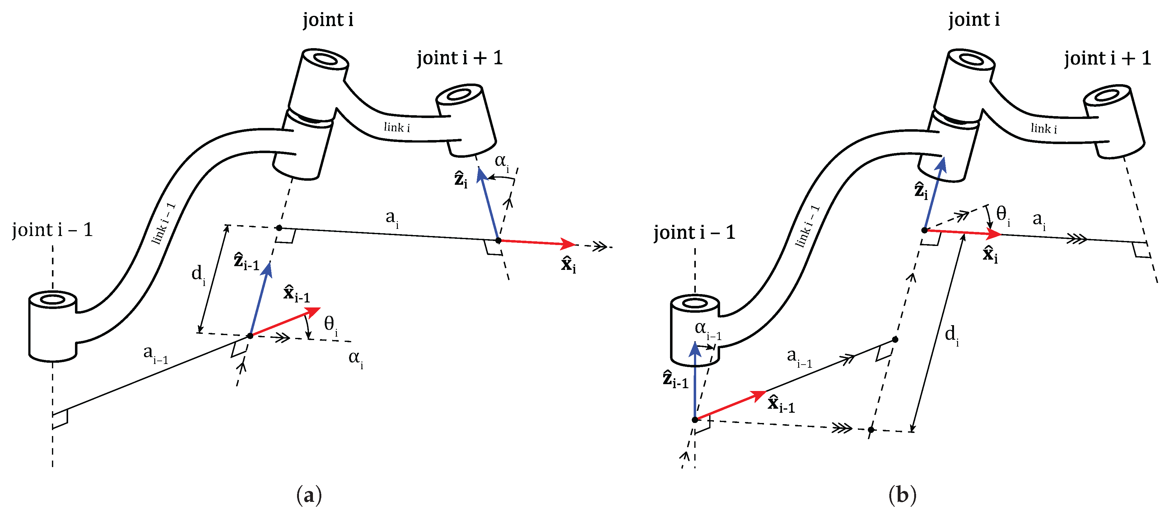
Figure 2.
Example on defining position and direction vector of a joint
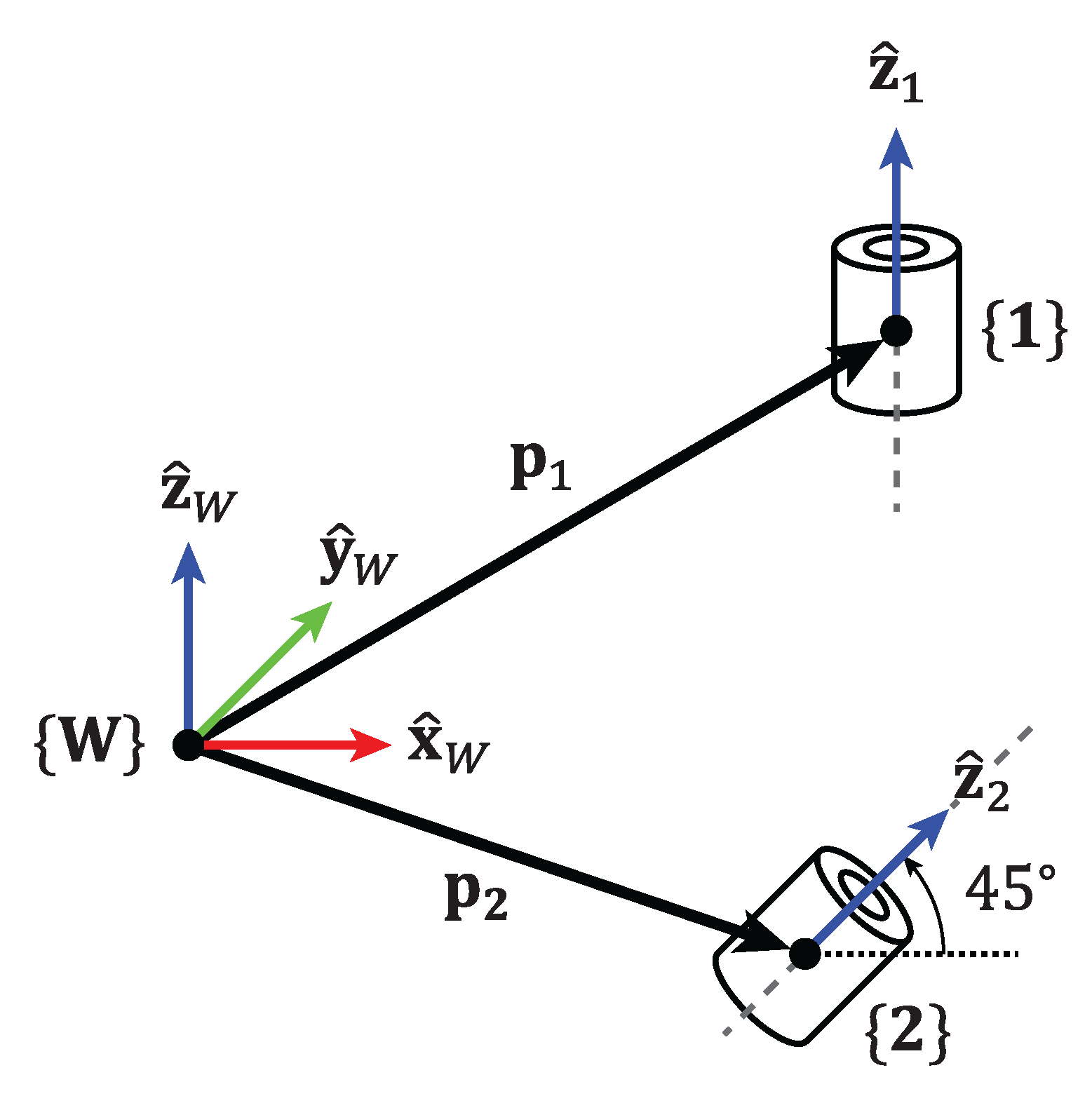
Figure 3.
Intersecting axes frame placement
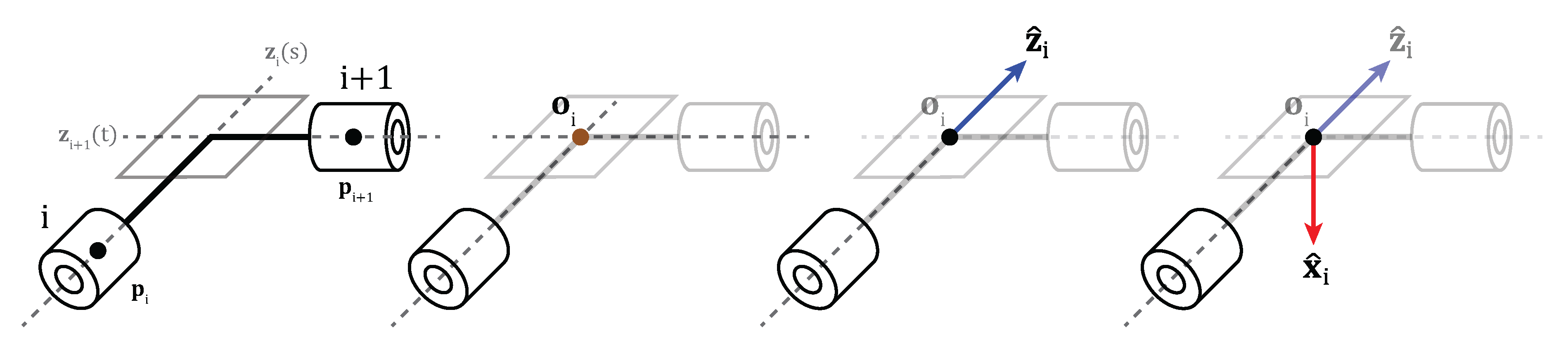
Figure 4.
Skew axes frame placement. Top: Isometric view. Bottom: Top view.
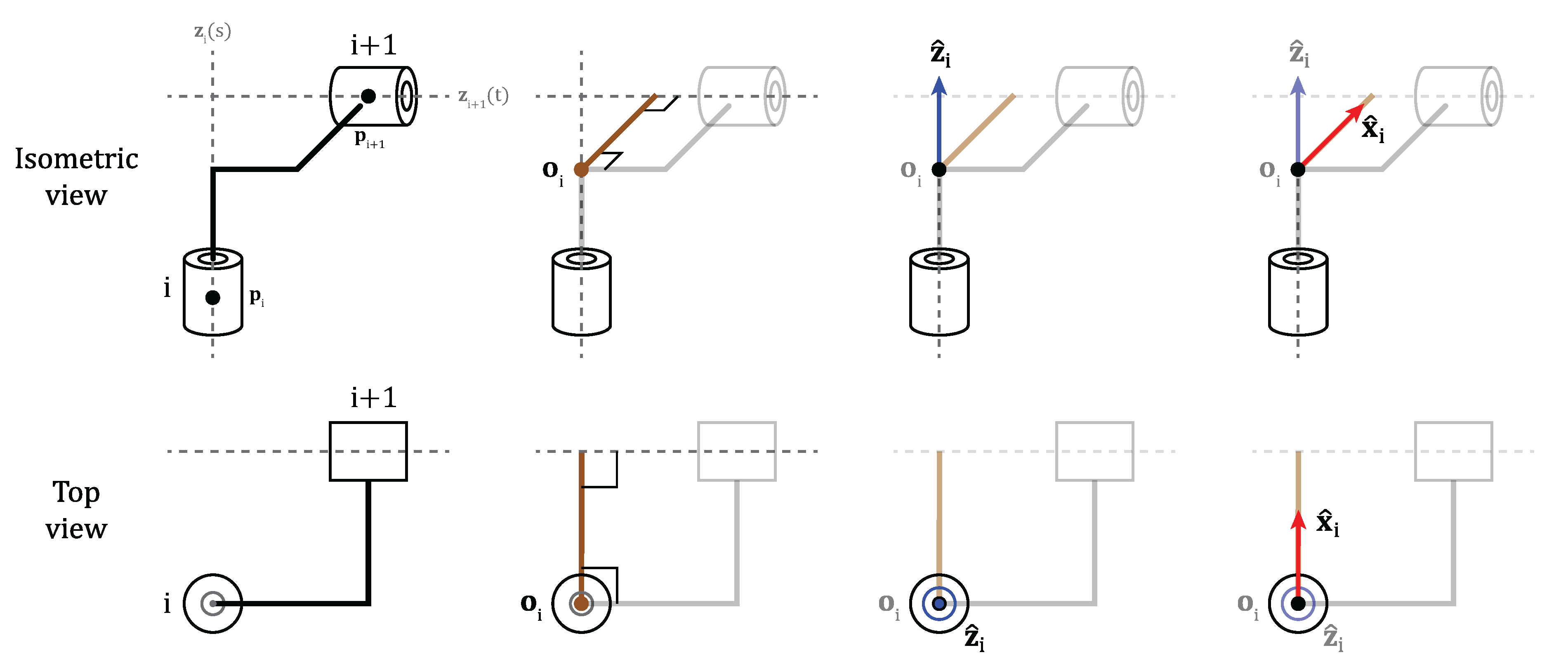
Figure 5.
Parallel axes frame placement
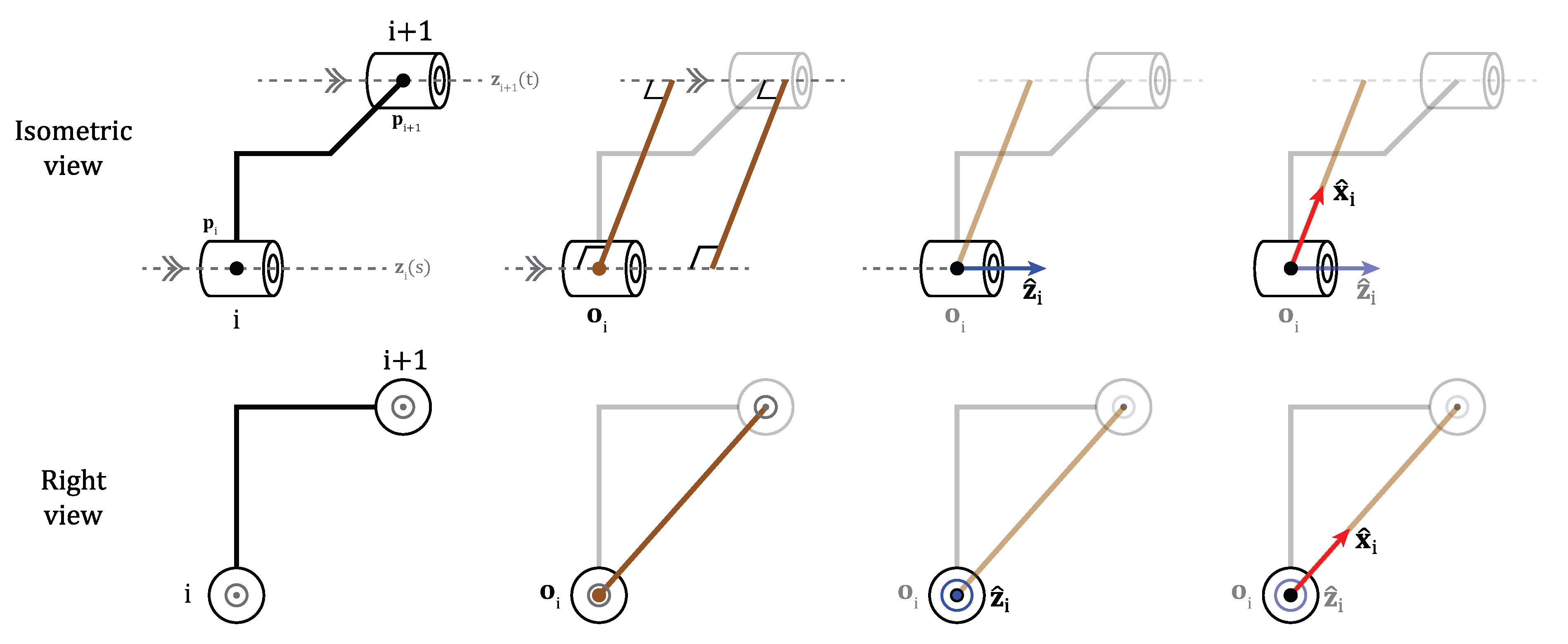
Figure 6.
Colinear axes frame placement
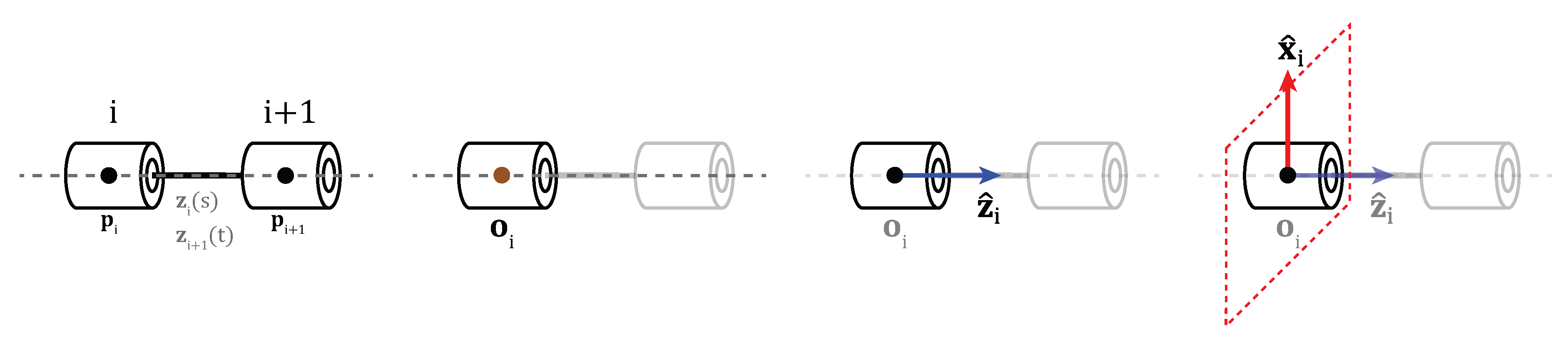
Figure 7.
Overview of the developed toolbox (a) Kinematics tab. (b) Workspace tab. (c) Volume Computation tab. (d) RoboDK Window.
Figure 7.
Overview of the developed toolbox (a) Kinematics tab. (b) Workspace tab. (c) Volume Computation tab. (d) RoboDK Window.
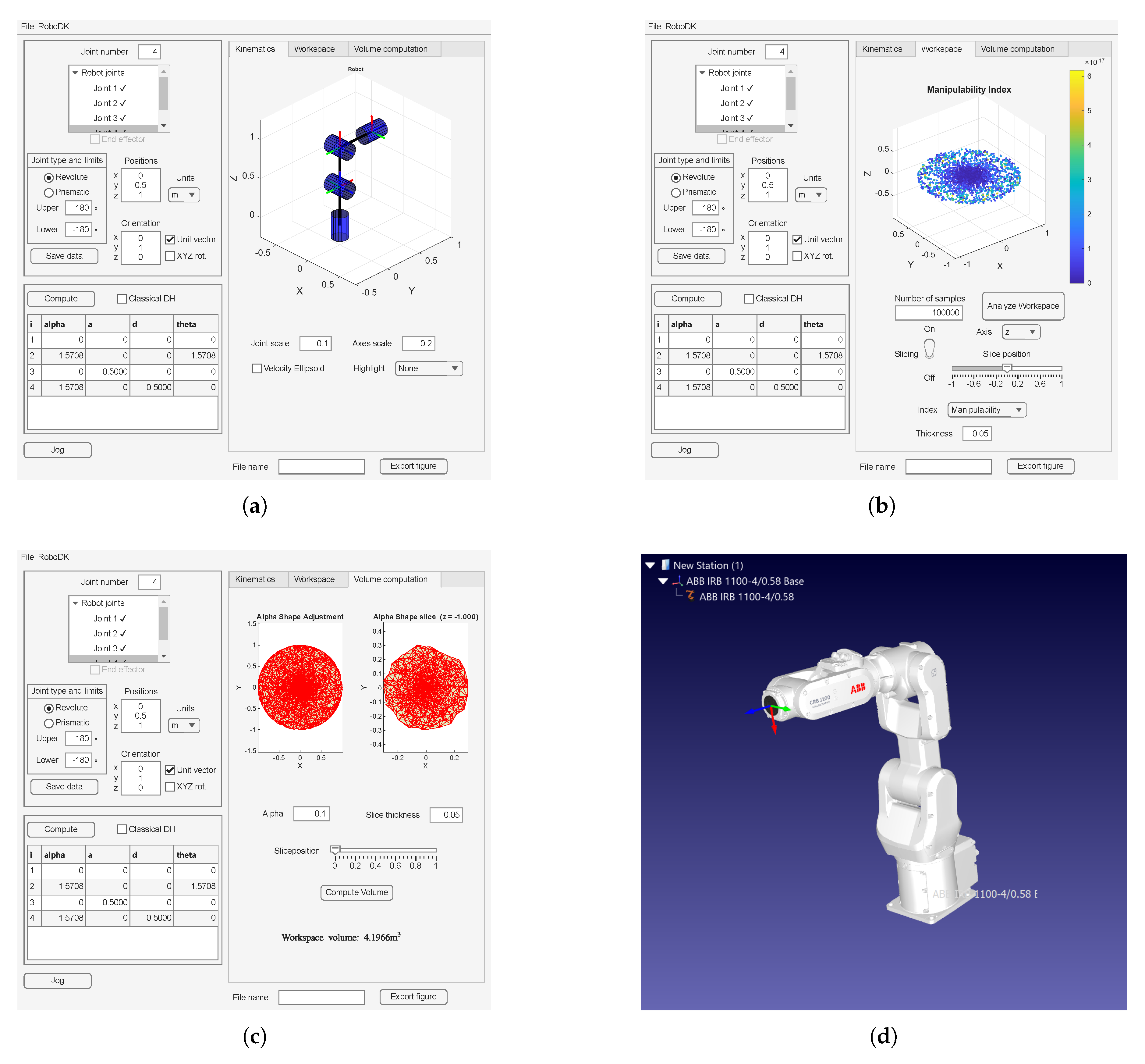
Figure 8.
MDH frame placement of the IRB 1100 (a) Full robot and frames. (b) Base and first joint frames. (c) Second joint frame. (d) Third joint frame. (e) Fourth joint frame. (f) Fifth joint frame. (g) Sixth joint frame.
Figure 8.
MDH frame placement of the IRB 1100 (a) Full robot and frames. (b) Base and first joint frames. (c) Second joint frame. (d) Third joint frame. (e) Fourth joint frame. (f) Fifth joint frame. (g) Sixth joint frame.
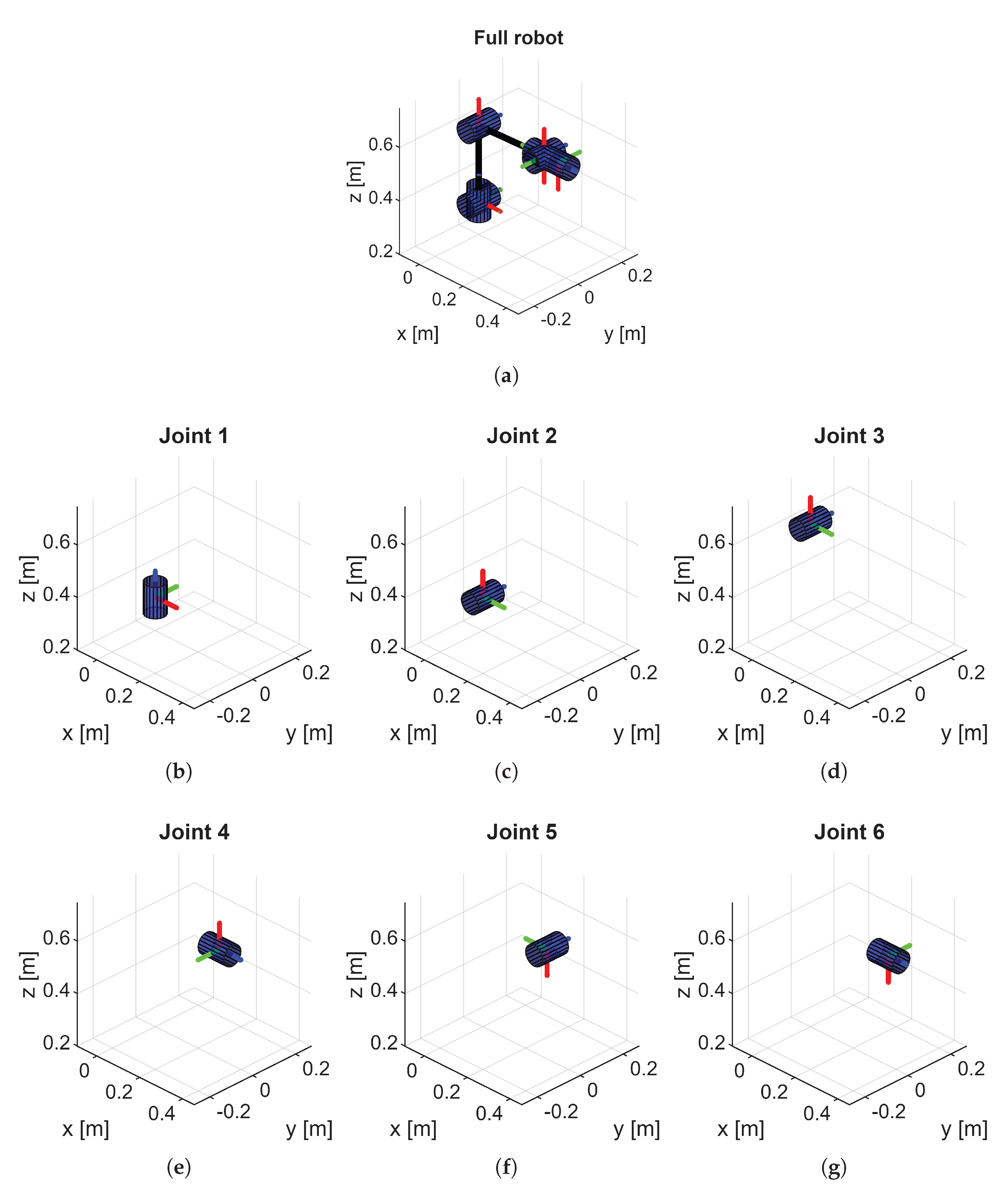
Figure 9.
MDH frame placement of the UR10e Robot (a) Complete robot and frame placements. (b) Base frame and first frame placement. (c) Second frame placement. (d) Third frame placement. (e) Fourth frame placement. (f) Fifth frame placement. (g) Sixth frame placement.
Figure 9.
MDH frame placement of the UR10e Robot (a) Complete robot and frame placements. (b) Base frame and first frame placement. (c) Second frame placement. (d) Third frame placement. (e) Fourth frame placement. (f) Fifth frame placement. (g) Sixth frame placement.
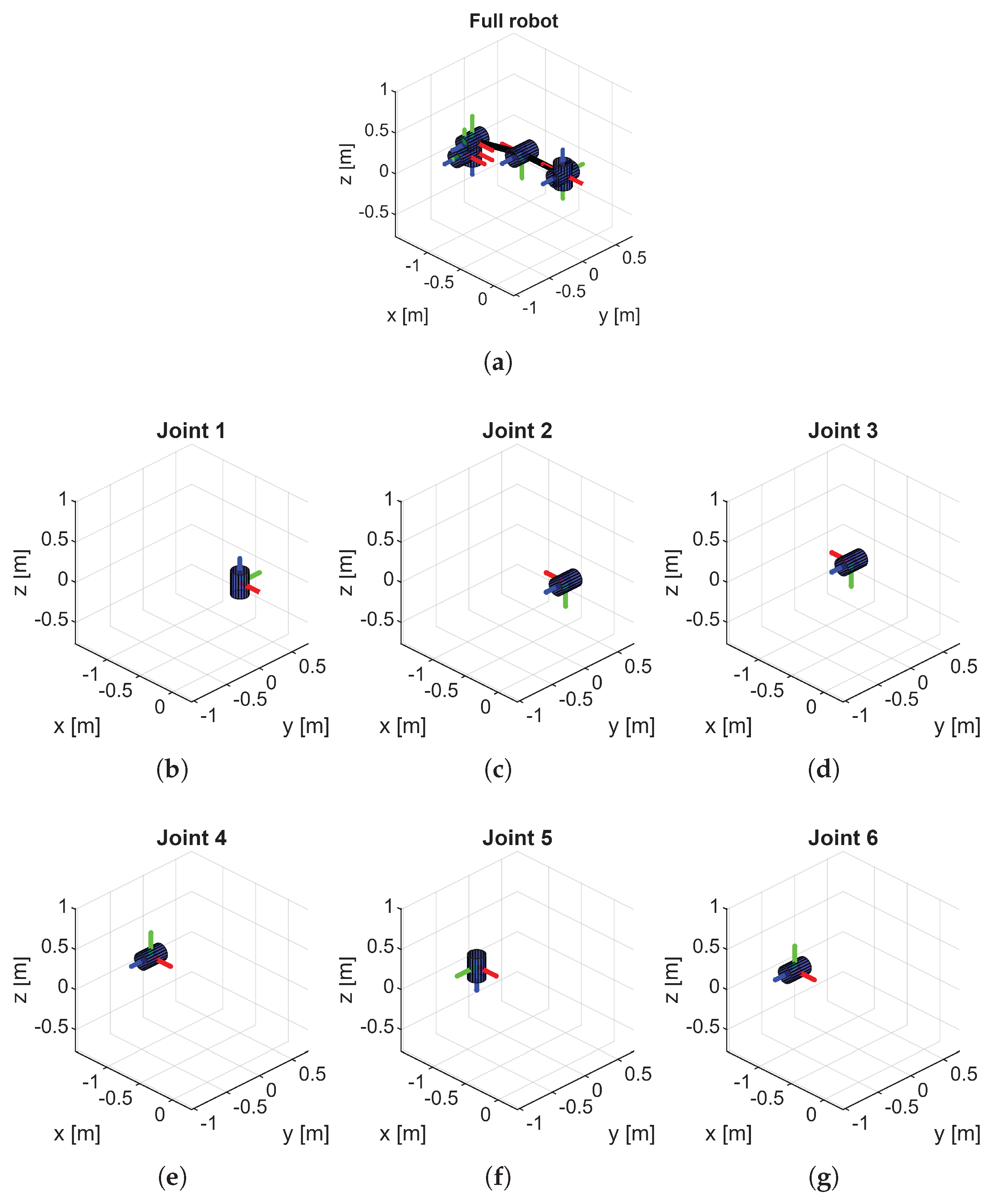
Figure 10.
Workspace analysis of the IRB 1100 (a) Slice of the xy plane. (b) Slice of the xz plane.
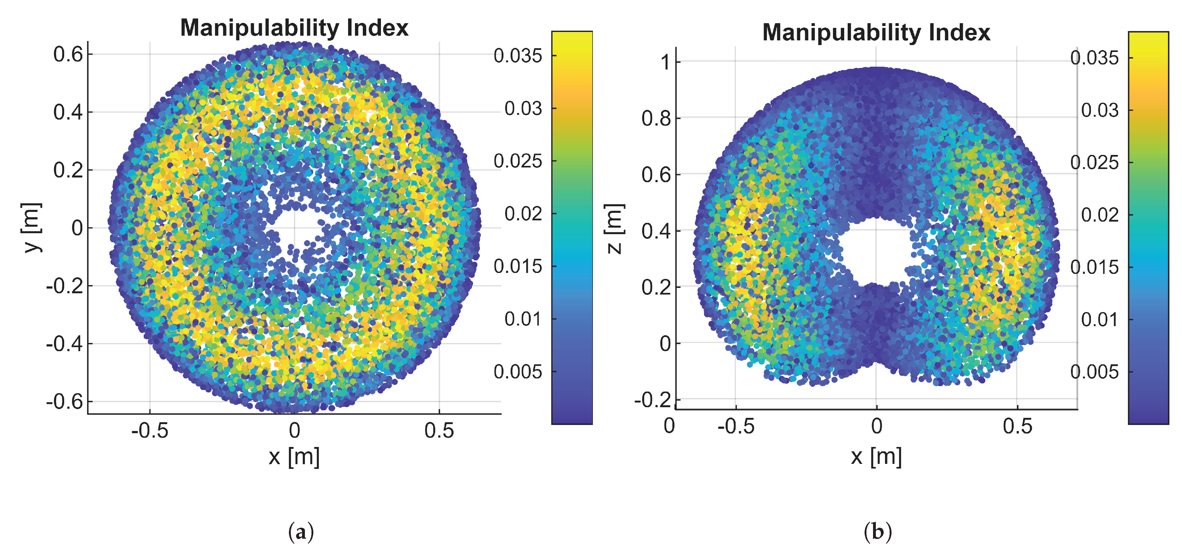
Figure 11.
Workspace dexterity analysis of the EPSON T3-401S (a) 3D overview. (b) Slice of the xz plane.
Figure 11.
Workspace dexterity analysis of the EPSON T3-401S (a) 3D overview. (b) Slice of the xz plane.
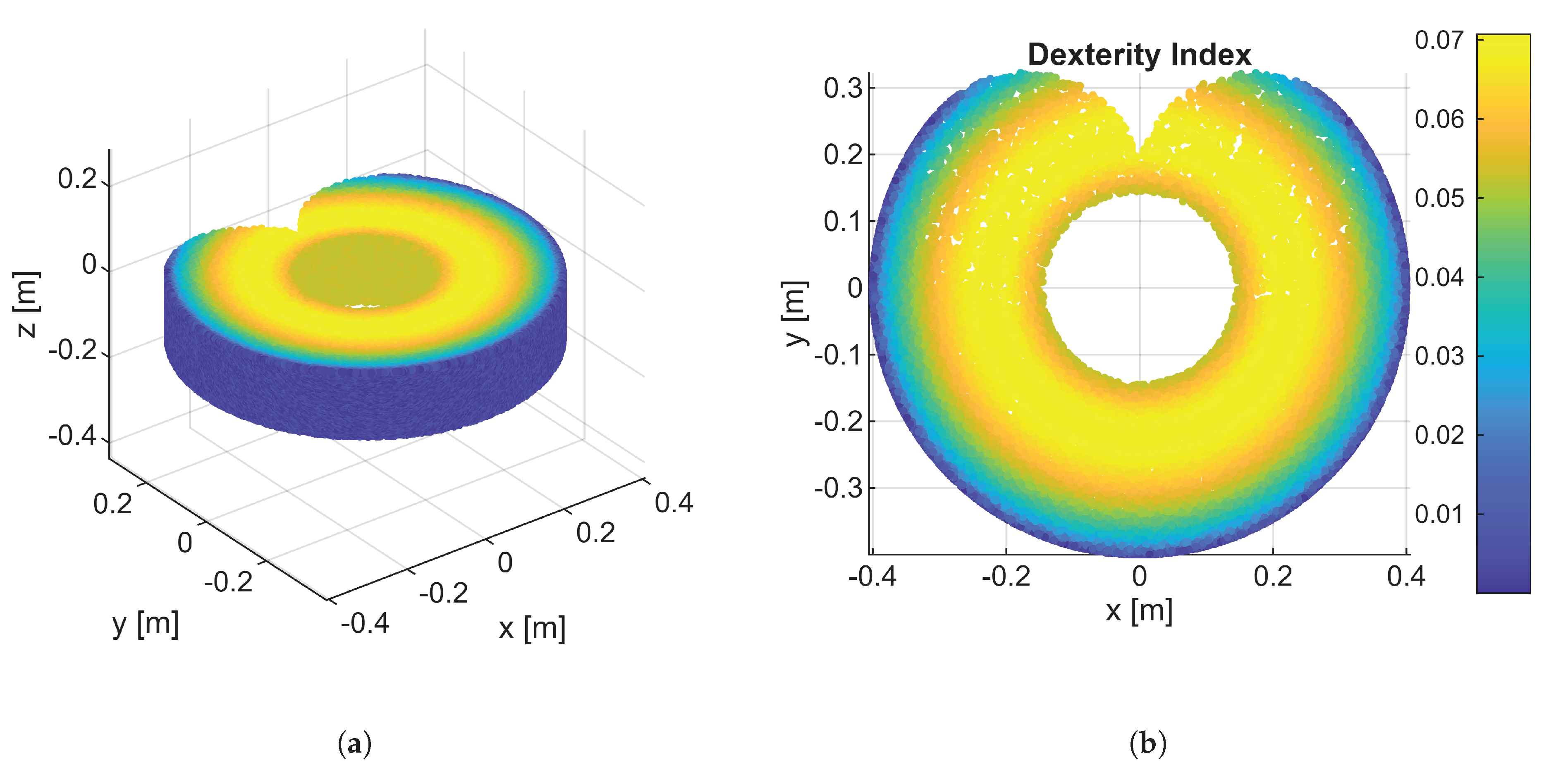

Table 1.
Classification of joint axis relationships based on Conditions C1–C3.
| Geometric Relationship | C1 | C2 | C3 |
|---|---|---|---|
| Intersecting | False | True | – |
| Skew | False | False | – |
| Parallel | True | – | False |
| Collinear | True | – | True |
Table 2.
IRB 1100 DH Parameters: RoboDK vs. Toolbox Modified
| Modified (RoboDK) | Modified (Toolbox) | |||||||
|---|---|---|---|---|---|---|---|---|
| Joint | [°] | [m] | [m] | [°] | [°] | [m] | [m] | [°] |
| 1 | 0 | 0.0000 | 0.3270 | 0 | 0 | 0 | 0.3270 | 0 |
| 2 | -90 | 0.0000 | 0.0000 | -90 | -90 | 0 | 0 | -90 |
| 3 | 0 | 0.2800 | 0.0000 | 0 | 0 | 0.2800 | 0 | 0 |
| 4 | -90 | 0.0100 | 0.3000 | 0 | -90 | 0.0100 | 0.3000 | 0 |
| 5 | 90 | 0.0000 | 0.0000 | 0 | 90 | 0 | 0 | 180 |
| 6 | -90 | 0.0000 | 0.0640 | 180 | 90 | 0 | 0.0640 | 0 |
Table 3.
UR10e DH Parameters: Manufacturer vs. Toolbox Classical and RoboDK Modified
| Classical (Manufacturer) | Classical (Toolbox) | |||||||
|---|---|---|---|---|---|---|---|---|
| Joint | [°] | [m] | [m] | [°] | [°] | [m] | [m] | [°] |
| 1 | 90 | 0.0000 | 0.1807 | 0 | 90 | 0.0000 | 0.1807 | 0 |
| 2 | 0 | -0.6127 | 0.0000 | 0 | 0 | 0.6126 | 0.0000 | 180 |
| 3 | 0 | -0.5716 | 0.0000 | 0 | 0 | 0.5713 | 0.0000 | 0 |
| 4 | 90 | 0.0000 | 0.1742 | 0 | 90 | 0.0000 | 0.1742 | -180 |
| 5 | -90 | 0.0000 | 0.1199 | 0 | -90 | 0.0000 | 0.1198 | 0 |
| 6 | 0 | 0.0000 | 0.1166 | 0 | 0 | 0.0000 | 0.1166 | 0 |
| Modified (RoboDK) | Modified (Toolbox) | |||||||
| Joint | [°] | [m] | [m] | [°] | [°] | [m] | [m] | [°] |
| 1 | 0 | 0.0000 | 0.1807 | 0 | 0 | 0.0000 | 0.1807 | 0 |
| 2 | 90 | 0.0000 | 0.0000 | 180 | 90 | 0.0000 | 0.0000 | 180 |
| 3 | 0 | 0.6126 | 0.0000 | 0 | 0 | 0.6126 | 0.0000 | 0 |
| 4 | 0 | 0.5713 | 0.1742 | 0 | 0 | 0.5713 | 0.1742 | -180 |
| 5 | -90 | 0.0000 | 0.1198 | 0 | 90 | 0.0000 | 0.1198 | 0 |
| 6 | 90 | 0.0000 | 0.1166 | 180 | -90 | 0.0000 | 0.1166 | 0 |
Table 4.
MDH Parameters: Slot Robot and Sphere Robot
| Slot Robot | Sphere Robot | |||||||
|---|---|---|---|---|---|---|---|---|
| Joint | [°] | [m] | [m] | [°] | [°] | [m] | [m] | [°] |
| 1 | 0 | 0.0000 | 0.0000 | 0 | 0 | 0.0000 | 1.0000 | 0 |
| 2 | 90 | 0.0000 | 0.0000 | 0 | 90 | 0.0000 | 0.0000 | 90 |
| 3 | 0 | 1.0000 | 0.0000 | 0 | 0 | 2.0000 | 0.0000 | 0 |
| 4 | 0 | 1.0000 | 0.0000 | 0 | 0 | 1.0000 | 0.0000 | 0 |
Table 5.
Workspace volume estimation results for different robots
| Robot Type | # Samples |
Slice Thickness [m] |
(Alpha-shape) |
Comp. Volume [m3] |
Real Volume [m3] |
Error [ % ] |
| Slot robot | 1,000k | 0.025 | ∞ | 41.1327 | 39.6795 | 3.5331 |
| Sphere robot | 1,000k | 0.020 | 0.35 | 108.3069 | 108.9085 | 0.5524 |
| Epson T3-401s | 500k | 0.004 | 0.02 | 0.058545 | 0.059873 | 2.2180 |
| ABB IRB 1400 | 1,000k | 0.0075 | 0.065 | 1.0186 | — | — |
| UR10e | 1,000k | 0.05 | 0.05 | 10.1194 | — | — |
| KUKA iiwa 7 | 5,000k | 0.01 | 0.1 | 3.0892 | — | — |
Disclaimer/Publisher’s Note: The statements, opinions and data contained in all publications are solely those of the individual author(s) and contributor(s) and not of MDPI and/or the editor(s). MDPI and/or the editor(s) disclaim responsibility for any injury to people or property resulting from any ideas, methods, instructions or products referred to in the content. |
© 2025 by the authors. Licensee MDPI, Basel, Switzerland. This article is an open access article distributed under the terms and conditions of the Creative Commons Attribution (CC BY) license (http://creativecommons.org/licenses/by/4.0/).
Copyright: This open access article is published under a Creative Commons CC BY 4.0 license, which permit the free download, distribution, and reuse, provided that the author and preprint are cited in any reuse.


