
Submitted:
23 March 2025
Posted:
24 March 2025
You are already at the latest version
Abstract
This work presents an alternative method for defining feasible joint-space boundaries and their corresponding geometric workspace in a planar robotic system. Instead of relying on traditional numerical approaches that require extensive sampling and collision detection, the proposed method constructs a continuous boundary by identifying key intersection points of boundary functions. The feasibility region is further refined through centroid-based scaling, addressing singularity issues and ensuring a structured trajectory. Comparative analyses demonstrate that the final robot pose and reachability depend on the selected traversal path, highlighting the nonlinear nature of the workspace. Additionally, an evaluation of traditional numerical methods reveals their limitations in generating continuous boundary trajectories. The proposed approach provides a structured method for defining feasible workspaces, improving trajectory planning in robotic systems.
Keywords:
planar robot
; feasible workspace
; self-collision constraints
; boundary functions
; trajectory planning
; geometric modeling
1. Introduction
The determination of feasible workspaces in robotic manipulators presents a fundamental challenge in robot design and control, requiring precise mathematical characterization of operational limits while ensuring collision-free configurations. Traditional methodologies primarily rely on numerical approaches that, although effective in estimating workspaces, often suffer from inefficiencies and lack precision when dealing with complex kinematic constraints. To address these issues, this work introduces a rigorous mathematical framework based on q-bound theorems, integrating geometric and kinematic constraints to enhance accuracy and computational efficiency in workspace determination.
Several numerical methods have been extensively studied for workspace analysis, including algorithms designed to map manipulator workspace boundaries, probabilistic numerical-analytical approaches [1], and Monte Carlo-based techniques [2]. These methodologies have been widely employed to approximate workspace limits and singularity regions, demonstrating effectiveness in various robotic configurations. For instance, the Monte Carlo method proposed enhances precision by leveraging Gaussian growth to refine workspace estimations. However, despite improving accuracy, its reliance on iterative random sampling limits its ability to produce continuous boundary trajectories. Similarly, the numerical algorithms developed by Haug et al. [3] employ a continuation method to systematically trace workspace boundaries, yet they require significant computational resources, particularly for kinematically redundant manipulators. Alternative strategies have been proposed to overcome these limitations, such as algebraic approaches for kinematic analysis [4] and probabilistic mapping methods for workspace determination [5].
Additionally, hybrid techniques have been explored to address workspace characterization. Li et al. [1] introduced a probabilistic approximation to generate boundary curves in workspaces; however, its dependency on randomization introduces potential inaccuracies, especially for manipulators with complex nonlinear constraints. Meanwhile, workspace determination methods for redundant manipulators, such as those proposed by Ginnante et al. [6], have been developed to reduce computational redundancy, but often struggle to precisely define workspace boundaries when joint configurations exceed a certain degree of redundancy.
Structural optimization techniques have also been investigated to enhance workspace determination. Cervantes-Sánchez et al. [7] formulated workspace generation as a direct kinematic problem, reducing computational complexity while maintaining accuracy in identifying singularity curves. Similarly, topology optimization methods [8] have been utilized to improve workspace efficiency, though they introduce additional complexities in parametric system optimization. Algebraic formulations [9] further support workspace evaluation, providing efficient solutions for robotic design in constrained environments.
Apart from geometric and numerical considerations, workspace feasibility is influenced by control strategies. The workspace observer method introduced by Oda et al. [10] presents a robust control strategy for redundant manipulators, focusing on real-time workspace regulation. However, such control-based approaches do not inherently define feasible workspaces and must be supplemented with mathematical workspace constraints, as examined in this study.
Alternative geometric transformations have also been proposed to tackle workspace determination challenges. The coverings transformation concept, explored by Rybak et al. [11], introduces an optimization-based method for approximating solutions to nonlinear inequalities that describe workspace constraints. Likewise, numerical approaches developed for parallel mechanisms [12] demonstrate that direct mapping techniques provide reliable workspace estimations but often involve significant computational loads. Structural synthesis methods [13] have also been introduced to systematically refine parallel robot architectures for improved workspace feasibility.
Another challenge in workspace determination involves identifying singularity curves and assembly configurations [7]. The characterization of singular configurations is essential for ensuring continuous, collision-free motion within the workspace, a concept that aligns with prior findings [3] where singular points were employed to construct precise workspace boundaries. Further studies on parasitic motion analysis [14] have provided insights into workspace constraints by leveraging constraint-embedded Jacobian formulations.
Furthermore, numerical ray-based methods, such as the one introduced by Ginnante et al. [6], offer an alternative approach for defining workspace limits in kinematically redundant manipulators. However, as noted by Ceccarelli [9], algebraic formulations provide more efficient methods for workspace evaluation and design.
To overcome the above mentioned limitations, this work proposes a mathematical formulation for defining feasible, collision-free workspaces through boundary functions that account for both geometric constraints and internal link interactions. This approach is particularly relevant for mechanisms with parallelogram structures, where geometric modeling plays a crucial role in improving workspace representation and ensuring the accurate detection of feasible regions, thereby mitigating inefficiencies associated with numerical sampling methods [15].
2. Theoretical Framework and Methodology
This section presents the theoretical framework and methodology for analyzing kinematic configurations and constraints in robotic manipulators. To ensure clarity in notation, vectors in will be represented as r, while rotation matrices in will be denoted as R. Mathematical conditions are derived to prevent internal collisions, forming the basis for defining feasible workspaces across robotic systems.
In the context of kinematic chains for robotic manipulators, each link is represented as a set of points. The principal nodes a and b define the positions of the joints that connect one link to the next. Any point on the current link can be labeled as , where n denotes the index of the point relative to the node a. Similarly, the node b connects to the subsequent link, and its points are labeled as . The purpose of this work is to establish the conditions under which a collision occurs between a point on the current link and a point on the subsequent link. An example of this kinematic configuration is illustrated in Figure 1.
In order to describe the feasible workspace, a boundary function is formulated as follows:
Here, represents the joint variables of the manipulator. The boundary function incorporates the following constraints:
- Kinematic Constraints: These ensure that joint variables respect their operational limits:
- Collision Avoidance Constraints: These prevent intersections between links by requiring a minimum separation distance between points and :
- Geometric Constraints: These define the external boundaries of the workspace based on the manipulator’s design:
Using these conditions, the boundary function serves as a mathematical tool to evaluate whether a configuration is valid and free from collisions.
The first step in ensuring that the manipulator operates safely and within a feasible workspace is to define the mathematical conditions under which collisions between links occur. These conditions are crucial for analyzing and understanding the interactions between the kinematic elements of the manipulator. The subsequent collision model generalizes these conditions, providing a foundational framework for identifying all potential collision scenarios. Finally, these generalized insights are used to construct boundary functions, which incorporate kinematic, collision avoidance, and geometric constraints to define the feasible workspace free of collisions.
To formalize the analysis, the following theorem generalizes the collision model for points within a kinematic chain.
Theorem 1.
Let the kinematic chain be defined, where 0 represents the base system, a and b are systems with variable position and orientation relative to each other, and and denote points with constant position and orientation within their respective local systems a and b.
A collision between the points and is said to occur if and only if the relative vector between these points equals a null vector:
this condition is equivalent to the norm of the relative vector being null:
under this condition, the relative position between the points is expressed as:
where is the rotation matrix that transforms coordinates from b to a, represents the relative position vector between a and b, denotes the local position of relative to a, and refers to the local position of relative to b. The condition for collision can also be expressed in terms of the boundary function , which depends on the joint variables . This boundary function is defined as:
A collision occurs if and only if:
The collision condition implies that all components of the vector are null, ensuring the positional coincidence of the points involved.
Proof of Theorem 1.
To derive the condition for a collision, we begin with the general formula for relative positions in a kinematic chain:
where is the relative vector between systems a and b, is the vector between a and , is the vector between and b, and is the rotation matrix that transforms coordinates from to a. While this relationship can be recursively extended for longer chains, we focus here on the consecutive points and for simplicity.
The relative position between and can be expressed as the difference between their global positions:
Using the transformations for global positions, we write:
Substituting these expressions into the relative position equation yields:
Simplifying this expression, we have:
Recognizing that can be rewritten as , we substitute and simplify:
Factoring out , we obtain:
The collision condition implies that the term in parentheses must also be null:
We now define the boundary function that encapsulates the condition for collision in terms of the joint variables :
Thus, a collision occurs if and only if:
This formulation ensures that the collision condition is expressed as a function of the joint variables, linking the geometry of the system to the kinematic configuration. Since the null vector ensures positional coincidence, the theorem is validated. □
Note that this approach facilitates a straightforward implementation of collision checks and the definition of boundaries, which are critical in the modeling of feasible workspaces and the optimization of manipulator trajectories. A significant simplification is achieved in the analysis of relative kinematic chains by avoiding the inherent complexity associated with homogeneous transformations and the Denavit-Hartenberg (DH) formalism. By focusing exclusively on the geometric relationships between consecutive systems, the need for complete transformation matrices is eliminated. Consequently, a more intuitive and computationally efficient model is provided, which is particularly advantageous in scenarios requiring rapid calculations and analytical clarity.
2.1. Case Study: Planar Robot
The Planar Robot is analyzed as a case study to illustrate the kinematic and collision constraints in robotic manipulators. Its structure consists of a two-degree-of-freedom mechanism, where and correspond to rotations about the y-axis. This configuration allows for a simplified representation of kinematic interactions while preserving essential characteristics for evaluating workspace feasibility and self-collision conditions. Figure 1 presents an isometric view of the robot, depicting its geometric arrangement and joint distribution.
This model is particularly useful for demonstrating the role of boundary conditions in defining feasible workspaces. The kinematic relationships between its links provide a structured approach for verifying self-collision criteria, as they depend on the relative positioning of consecutive elements in the manipulator’s chain. In this context, the feasible workspace is determined by considering the relative position vector between key reference points along the structure.
The kinematic chain of the Planar Robot, depicted in Figure 2, provides a structured representation of the positional relationships and rotational axes of its joints. The degrees of freedom are defined as follows:
- : Represents a rotational motion about the y-axis at the base.
- : Represents an additional rotation about the y-axis at the second joint, determining the final positioning of the end-effector.
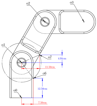
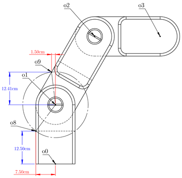
By formulating the manipulator’s motion in terms of relative position vectors and transformation matrices, it is possible to define a set of constraints that delineate the boundary of the feasible workspace. The self-collision condition is verified through a function that depends on the joint variables , ensuring that the relative displacement between reference points remains within allowable limits. The analysis of this system provides insight into the general methodology used to evaluate collision-free trajectories in robotic mechanisms. To support this analysis, Table 1 presents the geometric parameters that define the relative positioning of the robot’s joints, while Table 2 details the recursive formulation of the direct kinematics equations, describing the position and orientation of each joint in terms of preceding transformations.
3. Boundary Functions for Workspace Definition
The feasible workspace of the planar robot is determined by analyzing its geometric and kinematic constraints. To accurately characterize this workspace, boundary functions are derived to define the permissible motion range while preventing self-collisions. These functions capture the spatial relationships imposed by the robot’s structure, joint limits, and possible internal interferences. The formulation of these boundary conditions is guided by the theoretical framework established in Theorem 1, which provides the necessary conditions for detecting collisions within the kinematic chain. However, this theorem is not the sole tool employed in the analysis. Additional kinematic formulations, geometric considerations, and spatial transformations are integrated to comprehensively define the feasible workspace. The combination of these methods ensures a robust characterization of motion constraints, allowing for a detailed evaluation of collision-free configurations.
To systematically define these constraints, four tables are presented, each illustrating the computation of boundary functions along with a diagram marking critical collision points in the planar robot. These functions correspond to what are referred to as point boundary functions, where each function represents a specific constraint associated with a given collision point. In this type of boundary function, all components indexed by j must be satisfied simultaneously to confirm the occurrence of a collision. This simultaneous fulfillment is necessary because each corresponds to a different coordinate component, meaning that the collision is only valid when the spatial conditions for all coordinates hold true at the same time. By enforcing these constraints, it is possible to determine precise conditions under which the manipulator self-intersects at distinct locations in its configuration space.
In addition to these point boundary functions, a final table is included to introduce a different category of constraints known as geometric boundary functions. Unlike point boundary functions, these functions do not necessarily require all components to be satisfied simultaneously, as they do not define collisions at a discrete location but rather establish broader geometric constraints. Geometric boundary functions define spatial limits that the manipulator must respect, preventing it from exceeding predefined regions in its workspace. Since these constraints refer to entire geometric boundaries rather than discrete points, the conditions imposed by each function may be satisfied independently. This distinction highlights the difference between collision detection at specific points and the enforcement of global geometric restrictions that ensure safe operation.
The four tables presenting point boundary functions are labeled as Table 3, and Table 4. The final table, labeled as Table 5, provides the geometric boundary functions that define broader workspace constraints. Together, these boundary functions offer a structured method for computing the complete feasible workspace, ensuring that the manipulator operates within a collision-free region while supporting trajectory planning and operational reliability.
The boundary functions obtained from the previous analysis are presented as follows, encapsulating the constraints derived from the kinematic and geometric relationships of the planar robot. These functions define the conditions that must be satisfied to ensure a collision-free workspace while maintaining the feasible motion range of the manipulator.
To further characterize the motion constraints imposed by these boundary functions, the next step involves defining upper and lower bounds for each function. These bounds, denoted as , represent the k-th constraint imposed on the j-th component of the boundary function associated with the i-th collision condition. By establishing these bounds, the feasible motion range of the planar robot is precisely quantified, ensuring a structured approach to workspace determination.
Several of the boundary functions obtained in the analysis are expressed as linear combinations of cosine and sine terms. Therefore, it is necessary to establish a general method for determining the range of values that the variable q can assume while satisfying these constraints. The following theorem provides an explicit formulation for these bounds, enabling a systematic computation of the feasible joint configurations.
Theorem 2.
Given the equation of the form:
where are real numbers and q is the unknown variable to be determined, it follows that the solution for q is bounded by:
where accounts for the periodic nature of the trigonometric functions.
Proof of Theorem 2.
The given equation:
is rewritten using the trigonometric identity:
where d and are defined as:
By dividing both sides of the equation by d, it follows that:
For real solutions to exist, the term must satisfy the condition:
Taking the inverse cosine function on both sides, the expression:
is obtained. Solving for q, the result is:
Thus, it is concluded that q is bounded by:
This completes the proof. □
The upper and lower bounds for each boundary function are defined in Table 6. These bounds are established to determine the feasible range within which the functions operate, ensuring consistency in constraint evaluation. The right-bounded functions correspond to the upper limits, whereas the left-bounded functions define the lower limits, allowing for a comprehensive characterization of the solution space.
Figure 3 illustrates the graphical representation of the boundary functions. The red lines correspond to functions that are not considered in the construction of the feasible region, whereas the cyan lines represent the functions that define this region.
Although multiple feasible regions exist, reaching them from the home pose of the planar robot would require crossing or making contact with boundary functions, which would impose constraints on the motion. For this reason, the selection of the feasible region shown in the figure is justified.
As observed in Figure 3, the presence of multiple boundary functions complicates the identification of a unique solution. However, a feasible region can be constructed by identifying the intersection points of the selected boundary functions, forming a continuous boundary, as illustrated in Figure 4. This boundary is defined by six intersection points.
Nevertheless, the nonlinearities of certain functions prevent their respective constraints from being fully satisfied. This issue can be addressed through two possible approaches. The first approach involves incorporating additional tangent points along the sections of the functions where the constraints are not met. The second approach, as depicted in Figure 5, consists of computing the centroid of the feasible region and scaling it with respect to this point.
The latter approach also resolves an additional issue: while the boundary functions define the safe region, they inherently imply potential collisions. By applying a scaling factor, a safety margin is introduced between the robot and the boundary functions. This scaling coefficient acts as a safety factor, ensuring a collision-free operational space.
Figure 5 not only presents the closed and continuous boundary of the joint limits but also proposes a sequence for traversing these limits. However, Figure 6 illustrates the trajectory of these six intersection points in the geometric space, along with a simplified diagram of the planar robot in its final pose after completing the trajectory. It is important to note that although Figure 5 defines an ordered sequence for the boundary traversal, this does not inherently guarantee a structured or sequential trajectory in the geometric space.
Figure 7 presents two plots. The first illustrates a non-closed sequence of five points, while the second depicts the simplified diagram of the planar robot in its final pose after completing the trajectory. In this case, the trajectory is structured but remains open.
This phenomenon can be explained as follows: the workspace with the greatest reach is directly linked to the robot’s links when they become collinear. However, this configuration results in a joint singularity. This issue was indirectly resolved by scaling the feasible joint region with respect to its centroid, ensuring a structured path.
As a result, two distinct approaches exist for traversing the feasible geometric space along the right or the left side. This choice determines the final pose of the robot as well as its reach. Due to the limited workspace, the final link cannot transition to its mirrored pose within the same trajectory.
This second alternative is illustrated in Figure 8, which contains two plots. The first represents a joint trajectory consisting of five points, while the second shows the corresponding geometric trajectory. These paths are opposite to those presented in Figure 7.
The feasible geometric regions from Figure 7 and Figure 8 are overlaid in Figure 9. Notably, these regions do not exhibit symmetry, a result of the scaling applied relative to the centroid and the nonlinear properties inherent to the trajectory.
Figure 9 highlights the application of traditional numerical methods for solving this type of problem. Initially, a set of n random joint variables was generated. Following a conventional approach, each detected collision was marked with a red point, while non-colliding configurations were represented by blue points. These methods, however, entail a high computational cost and do not produce a continuous boundary trajectory in the joint space. Their efficiency is directly dependent on the volume of analyzed data.
Figure 9 presents two plots from this experiment: the first in the joint space and the second in the geometric space. In the latter, overlapping regions containing both collisions and non-collisions can be observed. This phenomenon is associated with the poses and trajectory patterns described in Figure 7 and Figure 8. Additionally, the lateral shapes of the geometric workspace, as seen in Figure 6, are also visible.
4. Conclusions
This study presented an alternative approach for defining feasible joint-space boundaries and their corresponding geometric workspace. Unlike traditional numerical methods, which rely on extensive sampling and collision detection, the proposed method constructs a continuous boundary by identifying and connecting critical intersection points of boundary functions.
The results demonstrate that scaling the feasible joint region with respect to its centroid resolves singularity issues and enables a structured path generation. Furthermore, the comparison of different trajectory alternatives highlights how the final pose and reachability of the robot depend on the selected traversal path.
Additionally, the overlay of feasible geometric regions confirms that symmetry is not preserved due to the nonlinearities and centroid-based scaling. The evaluation of traditional numerical methods further supports the advantages of the proposed approach, as random sampling methods result in high computational costs and fragmented boundaries.
Overall, the methodology introduced in this work provides a more efficient and structured solution for feasible workspace definition, offering improved trajectory continuity and computational efficiency in robotic motion planning.
Author Contributions
Conceptualization, J.A.L., L.F.L.-V. and H.A.G.-O.; methodology, J.A.L., E.L.-N. and M.E.M.-R.; software, D.M.N, and J.A.L.; validation, L.F.L-V., L.E.G.-J. and S.C.-T.; formal analysis, J.A.L. and R.C.-N;. investigation, D.M.N., S.C.-T. and M.E.M-R.; resources, J.A.L.; data curation and visualization, R.C.-N and J.A.L.; writing—original draft preparation, D.M.N. and J.A.L.; writing—review and editing, L.E.G.-J., L.F.L.-V. and H.A.G.-O.; visualization, D.M.N. and R.C.N; supervision, J.A.L, S.C.-T. and M.E.M.-R.; project administration, M.E.M.-R and J.A.L.; funding acquisition, J.A.-L. and E.L.-N. All authors have read and agreed to the published version of the manuscript.
Funding
The authors are thankful for the support of the Secretariat of Science, Humanities, Technology and Innovation (Secihti), through Project PCC-2022-319619 (“Project supported by Fondo Sectorial de Investigación para la Educación”).
Data Availability Statement
The data presented in this study are available on request from the corresponding author.
Conflicts of Interest
The authors declare no conflicts of interest.
References
- Li, X.J.; Cao, Y.; Yang, D.Y. A Numerical-Analytical Method for the Computation of Robot Workspace. In Proceedings of the The Proceedings of the Multiconference on "Computational Engineering in Systems Applications", 2006, Vol. 1, pp. 1082–1086. [CrossRef]
- Peidró, A.; Óscar Reinoso. ; Gil, A.; Marín, J.M.; Payá, L. An improved Monte Carlo method based on Gaussian growth to calculate the workspace of robots. Engineering Applications of Artificial Intelligence 2017, 64, 197–207. [Google Scholar] [CrossRef]
- Haug, E.J.; Luh, C.M.; Adkins, F.A.; Wang, J.Y. Numerical Algorithms for Mapping Boundaries of Manipulator Workspaces. Journal of Mechanical Design 1996, 118, 228–234, https://asmedigitalcollection.asme.org/mechanicaldesign/article-pdf/118/2/228/5920463/228_1.pdf. [Google Scholar] [CrossRef]
- Gallardo-Alvarado, J. Kinematic Analysis of Parallel Manipulators by Algebraic Screw Theory. Springer 2016. [Google Scholar]
- Kucner, T.P.; Lilienthal, A.J.; Magnusson, M.; Palmieri, L.; Swaminathan, C.S. Probabilistic Mapping of Spatial Motion Patterns for Mobile Robots. IEEE Robotics and Automation Letters 2020, 5, 1500–1507. [Google Scholar] [CrossRef]
- Ginnante, A.; Caro, S.; Simetti, E.; Leborne, F. Workspace Determination of Kinematic Redundant Manipulators Using a Ray-Based Method. Volume 8: 47th Mechanisms and Robotics Conference (MR), 2023. [Google Scholar]
- Cervantes-Sánchez, J.; Hernández-Rodríguez, J.; Rendón-Sánchez, J. On the workspace, assembly configurations and singularity curves of the RRRRR-type planar manipulator. Mechanism and Machine Theory 2000, 35, 1117–1139. [Google Scholar] [CrossRef]
- Wang, X.; Zhang, D.; Zhao, C.; Zhang, P.; Zhang, Y.; Cai, Y. Optimal design of lightweight serial robots by integrating topology optimization and parametric system optimization. Mechanism and Machine Theory 2019, 132, 48–65. [Google Scholar] [CrossRef]
- Ceccarelli, M. Workspace analysis and design of open-chain manipulators. AIP Conference Proceedings 1998, 437, 388–405, https://pubs.aip.org/aip/acp/article-pdf/437/1/388/12121917/388_1_online.pdf. [Google Scholar] [CrossRef]
- Oda, N.; Murakami, T.; Ohnishi, K. A Robust Control Strategy of Redundant Manipulator by Workspace Observer. Journal of Robotics and Mechatronics 1996, 8, 235–242. [Google Scholar] [CrossRef]
- Rybak, L.A.; Behera, L.; Averbukh, M.A.; Sapryka, A.V. A novel approach for coverings transformation to define a robot workspace. IOP Conference Series: Materials Science and Engineering 2020, 945, 012075. [Google Scholar] [CrossRef]
- Zhou, Y.; Niu, J.; Liu, Z.; Zhang, F. A novel numerical approach for workspace determination of parallel mechanisms. Journal of Mechanical Science and Technology 2017, 31, 3005–3015. [Google Scholar] [CrossRef]
- Gogu, G. Structural Synthesis of Parallel Robots, Part 1: Methodology. Springer 2008. [Google Scholar]
- Nigatu, H.; Choi, Y.H.; Kim, D. Analysis of Parasitic Motion with the Constraint Embedded Jacobian for a 3-PRS Parallel Manipulator. Mechanism and Machine Theory 2021, 157, 104181. [Google Scholar] [CrossRef]
- Merlet, J.P. Parallel Robots. Springer 2006. [Google Scholar]
Figure 1.
Illustration of a kinematic chain is presented as a simplified example of a planar robot. The nodes a and b indicate the joint positions connecting consecutive links, while the points and are identified as collision points between adjacent links.
Figure 1.
Illustration of a kinematic chain is presented as a simplified example of a planar robot. The nodes a and b indicate the joint positions connecting consecutive links, while the points and are identified as collision points between adjacent links.
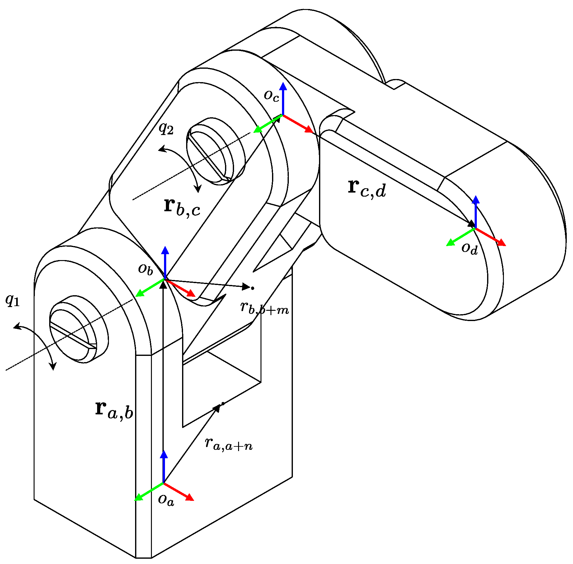
Figure 2.
Representation of the kinematic chain for MinervaBotV2.
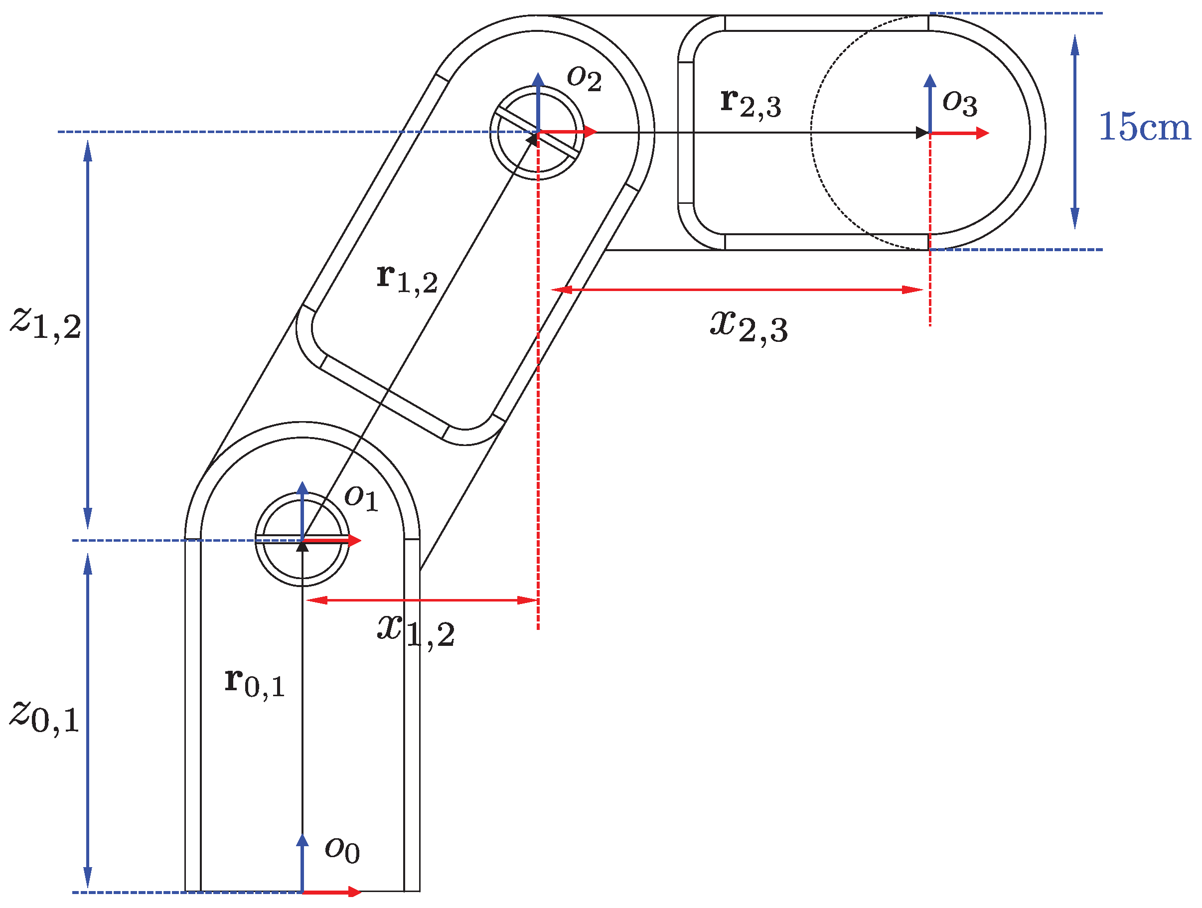
Figure 3.
Graphical representation of the boundary functions. Red lines indicate functions that are not considered in defining the feasible region, while cyan lines represent the functions used to construct it. The selected feasible region is determined by the boundary functions , , , , , and .
Figure 3.
Graphical representation of the boundary functions. Red lines indicate functions that are not considered in defining the feasible region, while cyan lines represent the functions used to construct it. The selected feasible region is determined by the boundary functions , , , , , and .
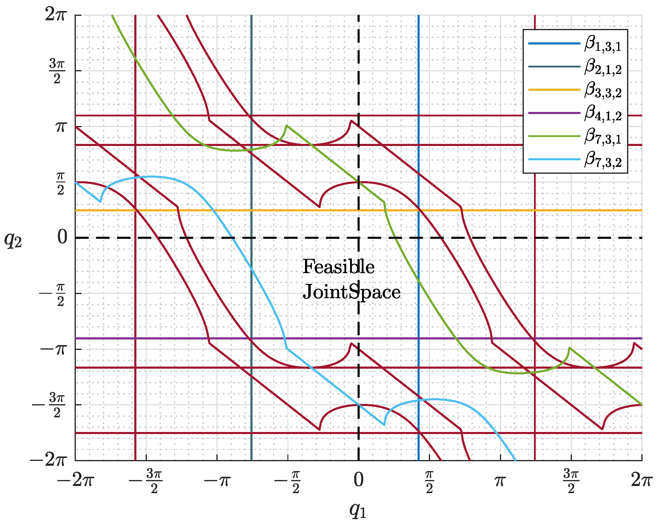
Figure 4.
Construction of the feasible region by identifying the intersection points of the selected boundary functions. The continuous boundary is formed by six intersection points, ensuring a well-defined feasible area for the robot’s motion.
Figure 4.
Construction of the feasible region by identifying the intersection points of the selected boundary functions. The continuous boundary is formed by six intersection points, ensuring a well-defined feasible area for the robot’s motion.
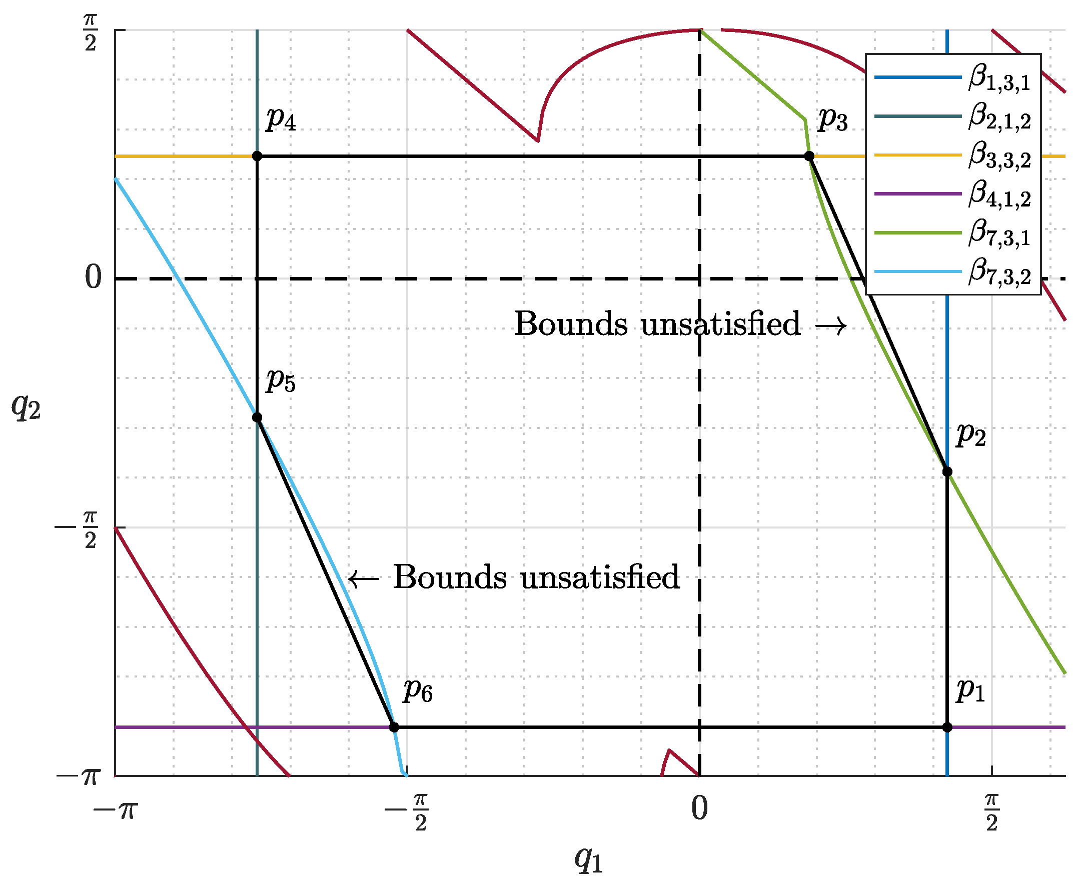
Figure 5.
Scaling of the feasible region with respect to its centroid. This approach ensures that the boundary functions do not directly imply collision while introducing a safety margin for the robot’s operation. The scaling factor acts as a safeguard to maintain a collision-free workspace.
Figure 5.
Scaling of the feasible region with respect to its centroid. This approach ensures that the boundary functions do not directly imply collision while introducing a safety margin for the robot’s operation. The scaling factor acts as a safeguard to maintain a collision-free workspace.
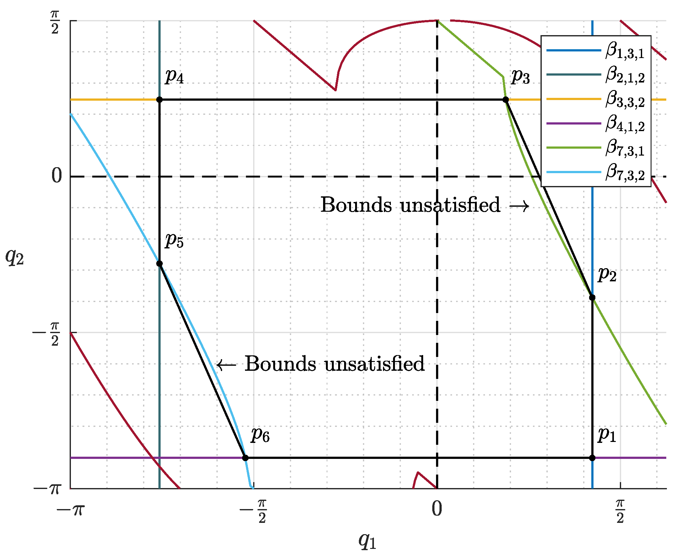
Figure 6.
Trajectory of the six intersection points in the geometric space, including the simplified diagram of the planar robot in its final pose.
Figure 6.
Trajectory of the six intersection points in the geometric space, including the simplified diagram of the planar robot in its final pose.
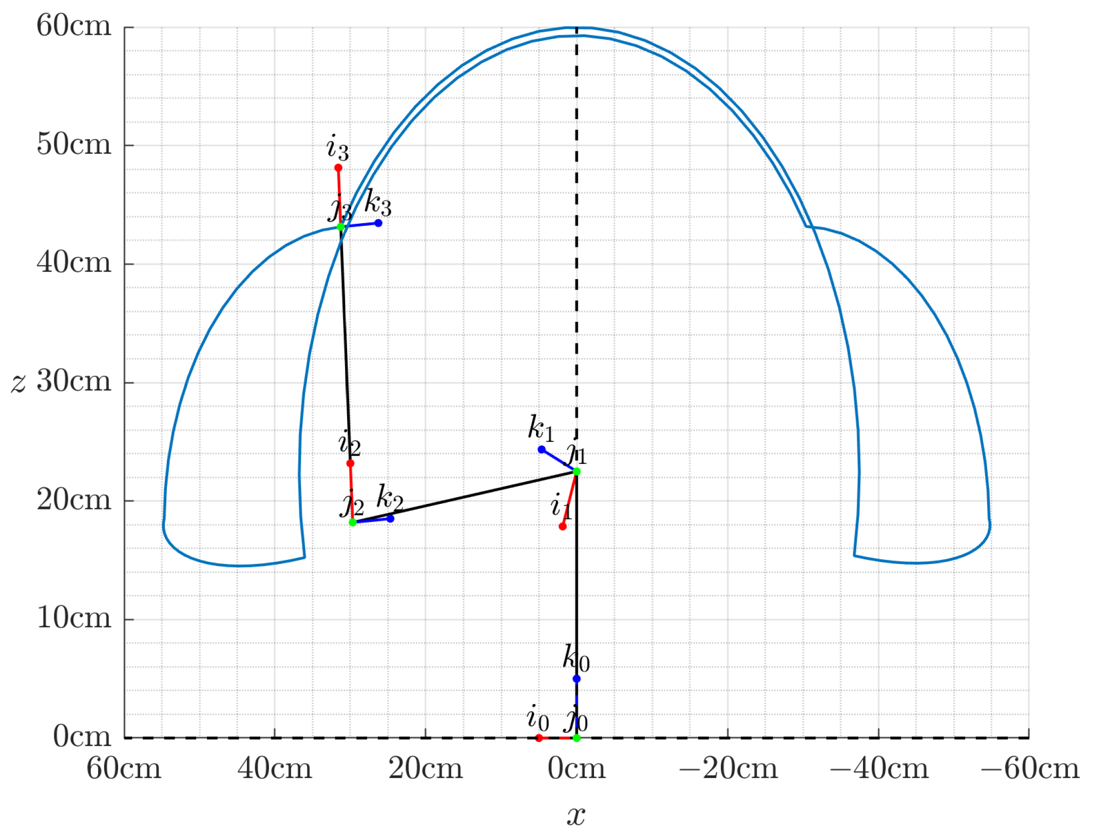
Figure 7.
Non-closed trajectory consisting of five points. The first plot represents the joint space sequence, while the second illustrates the planar robot in its final pose after completing the trajectory. Despite following an ordered sequence, the trajectory remains open.
Figure 7.
Non-closed trajectory consisting of five points. The first plot represents the joint space sequence, while the second illustrates the planar robot in its final pose after completing the trajectory. Despite following an ordered sequence, the trajectory remains open.
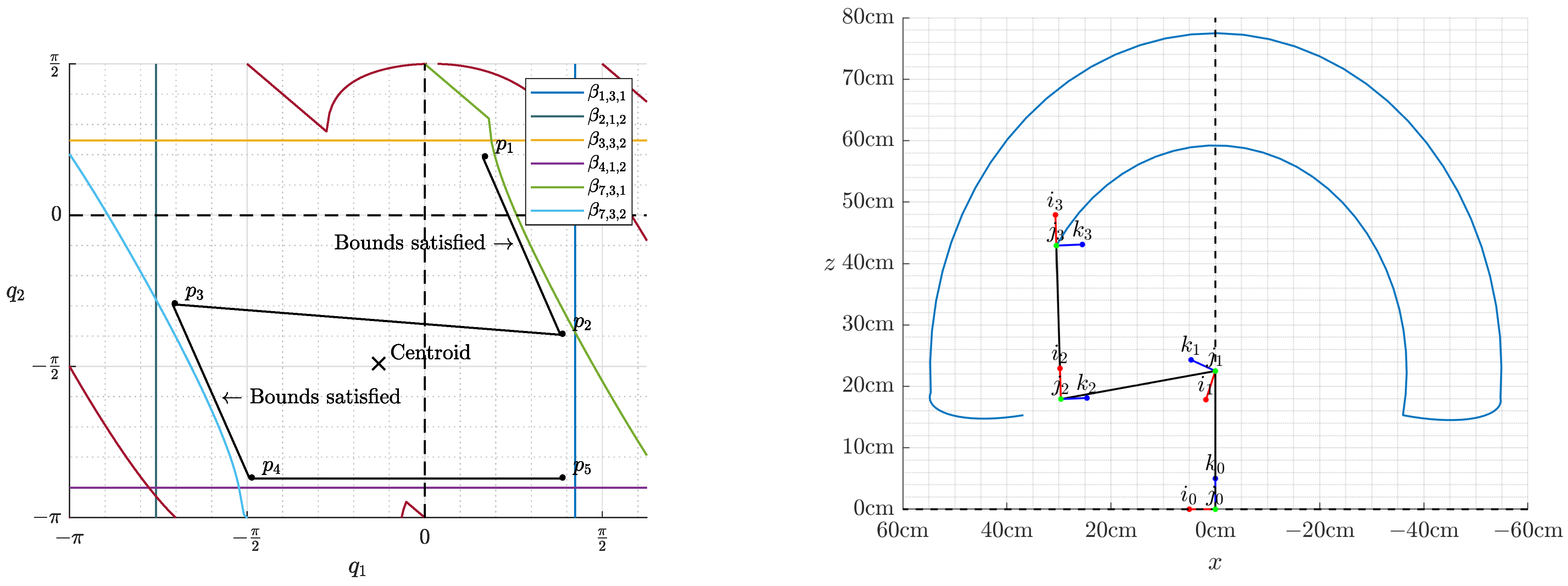
Figure 8.
Alternative feasible trajectory. The first plot depicts a five-point joint space path, while the second shows its corresponding geometric trajectory.
Figure 8.
Alternative feasible trajectory. The first plot depicts a five-point joint space path, while the second shows its corresponding geometric trajectory.
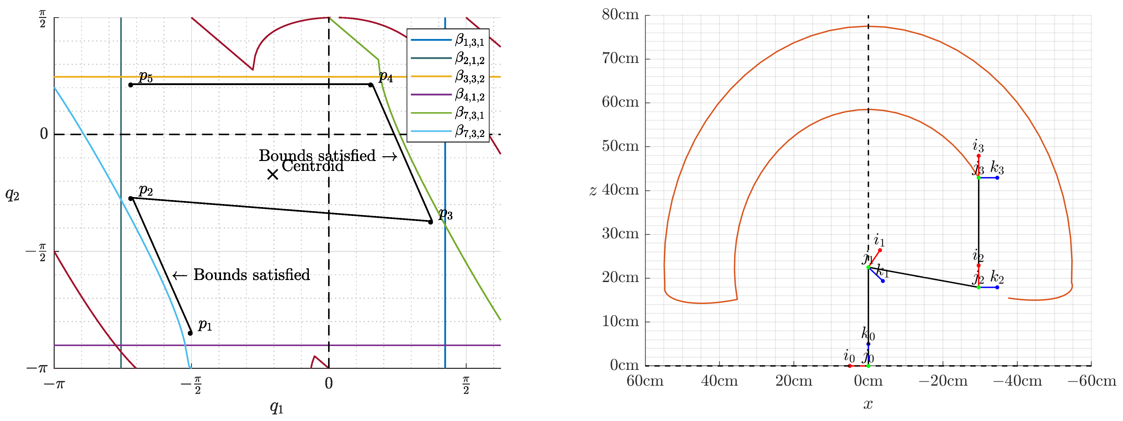
Figure 9.
Overlay of the feasible geometric regions from Figure 7 and Figure 8, highlighting their asymmetry due to centroid-based scaling and trajectory nonlinearities.
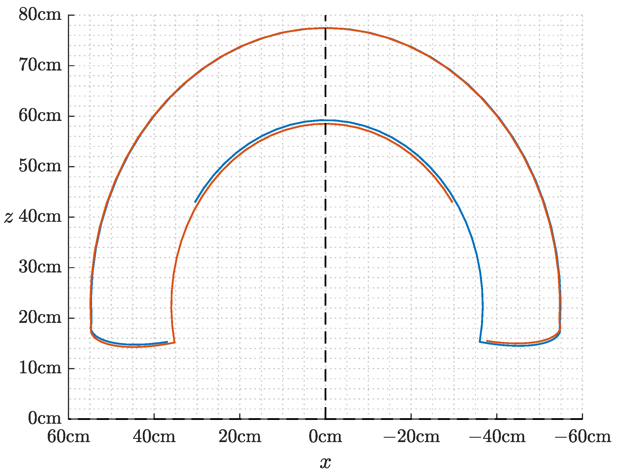
Figure 10.
Numerical collision detection results. The first plot shows joint space sampling with red points for collisions and blue points for non-collisions. The second plot illustrates the corresponding geometric space, highlighting overlapping regions and the lateral shapes of the feasible workspace.
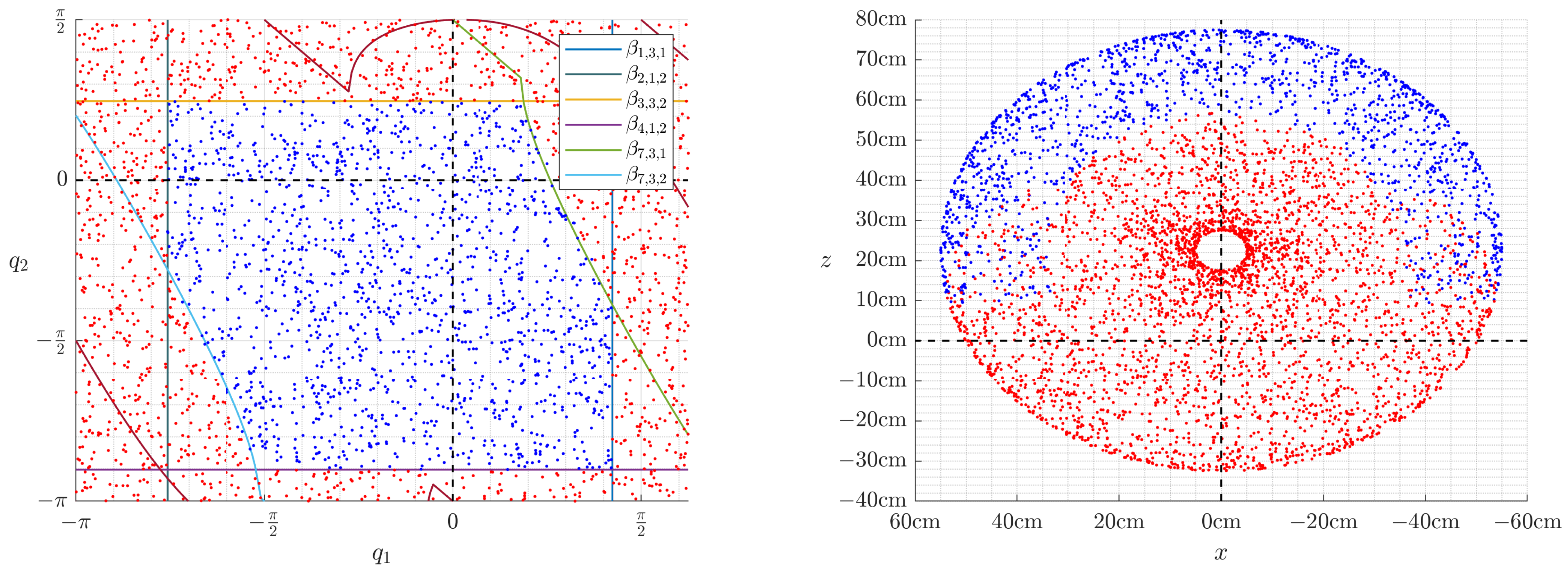

Table 1.
Geometric offsets of Planar Robot.
| frames Connected | Parameter | Symbol | Value (cm) |
| Offset z (Base to Joint 1) | 22.5 | ||
| Offset z (Joint 1 to Joint 2) | 25.98 | ||
| Offset x (Joint 1 to Joint 2) | 15 | ||
| Offset x (Joint 2 to Joint 3) | 25 |
Table 2.
Direct kinematics equations, recursive notation.
| Point | Position Vector | Matrix | Orientation |
|---|---|---|---|
| I | |||
| I | |||
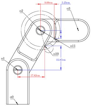
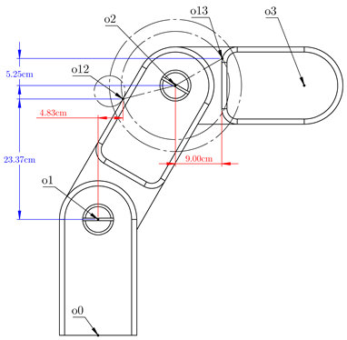
Table 3.
Point Boundary Function 1, 2 and 3.
| Graphic | Geometric offsets and Boundary functions |
|---|---|
 |
|
 |
|
 |
|
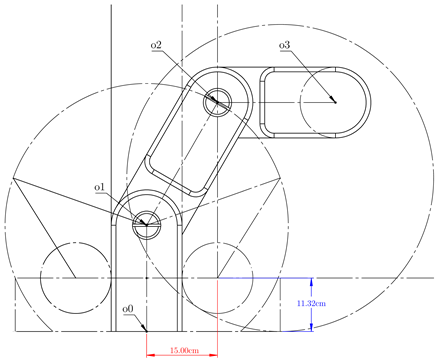
Table 4.
Point Boundary Function 4.
| Graphic | Geometric offsets and Boundary functions |
|---|---|
 |
|
Table 5.
Geometric Boundary Function 5, 6 and 7.
| Graphic | Geometric offsets and Boundary functions |
|---|---|
 |
|
Table 6.
Boundary function bounds.
| Right Bounded Function | Left Bounded Function | |
|---|---|---|
Disclaimer/Publisher’s Note: The statements, opinions and data contained in all publications are solely those of the individual author(s) and contributor(s) and not of MDPI and/or the editor(s). MDPI and/or the editor(s) disclaim responsibility for any injury to people or property resulting from any ideas, methods, instructions or products referred to in the content. |
© 2025 by the authors. Licensee MDPI, Basel, Switzerland. This article is an open access article distributed under the terms and conditions of the Creative Commons Attribution (CC BY) license (http://creativecommons.org/licenses/by/4.0/).
Copyright: This open access article is published under a Creative Commons CC BY 4.0 license, which permit the free download, distribution, and reuse, provided that the author and preprint are cited in any reuse.


