
Submitted:
17 December 2024
Posted:
18 December 2024
You are already at the latest version
Abstract
Aiming at the problems of six-degree-of-freedom robotic arm in three-dimensional multi-obstacle space, such as low sampling efficiency and path search failure, an improved fast extended random tree (RRT*) algorithm for robotic arm path planning method (abbreviated as HP-APF-RRT*) is proposed. The algorithm generates multiple candidate points per iteration, selecting a sampling point probabilistically based on heuristic values, thereby optimizing sampling efficiency and reducing unnecessary nodes. To mitigate increased search times in obstacle-dense areas, an Artificial Potential Field (APF) approach is integrated, establishing gravitational and repulsive fields to guide sampling points around obstacles toward the target. This method enhances path search in complex environments, yielding near-optimal paths. Furthermore, the path is simplified using the triangle inequality, and redundant intermediate nodes are utilized to further refine the path. Finally, the simulation experiment of the improved HP-APF-RRT* is executed on the Matlab and ROS, and the physical experiment is done on the NZ500-500 robotic arm. The effectiveness and superiority of the improved algorithm are deter-mined by comparing it with the existing algorithms.
Keywords:
six-degree-of-freedom robotic arm
; path planning
; RRT*
; APF
; triangular inequalities
1. Introduction
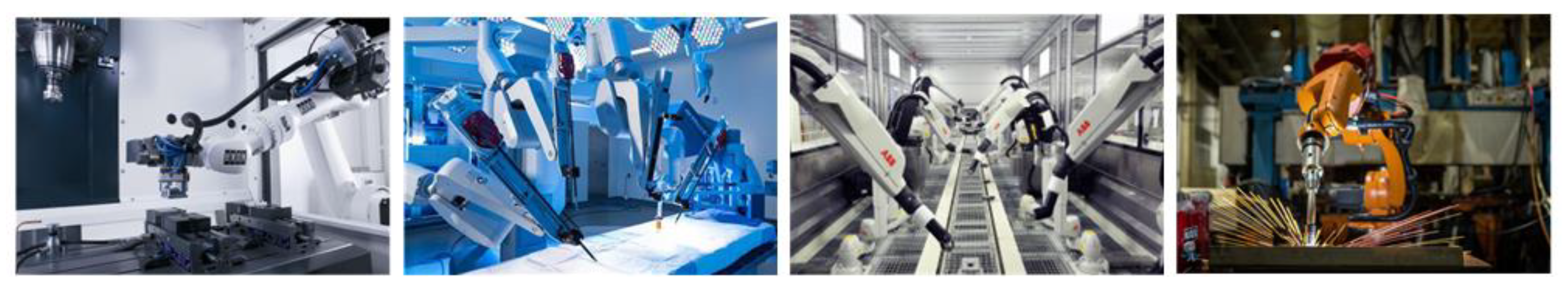
The six-degree-of-freedom manipulator plays a crucial role in modern manufacturing, healthcare, service, and logistics. With the rapid advancement of automation technology, the application scenarios for robotic arms have become increasingly complex, necessitating their ability to perform multiple tasks efficiently and safely in dynamic and uncertain environments[1]. Path planning, as the core problem of robotic arm motion control, aims to generate a feasible path for the robotic arm from the start position to the target position. Simultaneously, it is essential to ensure that the path avoids collisions with obstacles present in the environment throughout the motion[2].
Figure 1.
Industrial robot.
Path planning algorithms can be categorized into two types: search-based path planning algorithms and sampling-based path planning algorithms[3]. Search-based path planning algorithms, such as Dijkstra[4] and the A* algorithm[5], determine the optimal path from a starting point to an endpoint by exploring a discrete state space. They typically operate on a grid or grid graph, constructing a state space graph by connecting adjacent states, and executing pathfinding based on this structure.Although these algorithms demonstrate strong performance in simple environments, they frequently encounter challenges, including low computational efficiency and unsmooth paths in high-dimensional spaces and complex obstacle environments[6]. Unlike search-based algorithms, sampling-based path-planning algorithms, such as Rapidly Exploring Random Trees (RRT) [6]and Probabilistic Roadmaps (PRM)[7], generate paths by randomly sampling points within the state space. They are generally regarded as probabilistically complete. If a path exists, the algorithm can certainly identify a feasible route over time. Even if the PRM is theoretically complete, it encounters several challenges in practical applications.These challenges include low efficiency, time-consuming collision detection, a lack of consideration for the robot's kinematic model, and efficiency losses associated with the two-stage method[8,9]. In addition, the PRM offers probabilistic completeness but does not guarantee optimality. Despite the RRT is effective in navigating high-dimensional spaces, it has several drawbacks. These include significant randomness, slow search speeds in environments with complex obstacles, and the generation of non-optimal planning paths[10,11].
In order to address the issue of the large number of nodes and non-optimal paths generated by the RRT, Karaman et al. [12]proposed the RRT*. The algorithm incorporates a cost function based on RRT. It reduces the randomness of the final path by eliminating the selection of the parent node, which results in asymptotic optimality; however, this approach increases the planning time. Adiyatov et al. [13]proposed a rapid exploration algorithm known as the Randomized Tree Fixed Nodes (RRT*FN). The algorithm restricts the maximum number of nodes, and its methods for sampling, node expansion, and parent selection are consistent with those of the RRT* . Although this method prevents the infinite growth of the tree and conserves memory, it does not significantly enhance planning speed, and the convergence accuracy remains low. To address the issue of the prolonged execution time of the RRT*, Lavalle et al. [14]proposed the bidirectional extended randomized tree algorithm, Bi-RRT. The algorithm enhances pathfinding by extending it from both directions, significantly improving the efficiency of search and path planning. Zhou et al.[15] developed a novel strategy for searching nearest neighbors, known as the generalized distance method, which significantly reduces search time. Aiming at the issue of blind node sampling in the RRT* algorithm, Yi et al. [16]proposed an enhanced version known as the improved P-RRT * algorithm based on RRT * ( improved P-RRT * ). The enhanced P-RRT* employs two expansion methods for generating new nodes, thereby improving the algorithm's search efficiency. The first extension employs a target bias extension strategy. The second extension utilizes a random sampling strategy within rectangular regions. Fazhan Tao et al. [17]influenced the generation of random sampling points by introducing a variable probability target bias strategy. Combining enhanced artificial potential field methods with growing trees significantly improves the search speed and path quality of randomized trees and reduces the generation of invalid nodes. Wang et al.[18] utilized Gaussian mixed regression to identify key features in human demonstrations, thereby creating a probability density distribution of human trajectories. It is used to guide the sampling process, enabling the rapid generation of feasible paths. In light of the issue of slow search speeds in narrow regions, Wang et al. [19]proposed the NRRT*. The methodology utilizes the optimal paths derived from the A* algorithm as the training set. It guides the expansion and path search processes are enhanced by leveraging the predictive and optimization capabilities of neural networks, which facilitate a more efficient sampling process in narrow spaces. Q.C. [20]proposed the RJ-RRT. It employs a novel greedy sampling space reduction strategy along with an environmental assessment approach. The method reduces redundant nodes while accelerating the expansion of the random tree toward the target region. It can identify narrow passages and utilizes subtrees to explore these passages internally.
Although previous studies have made significant progress in enhancing the perfor-mance of the RRT* algorithm, they have not thoroughly examined its applicability in three-dimensional complex spatial environments. Therefore, this paper proposes an RRT* robotic arm path planning algorithm that integrates heuristic probabilistic sampling with the artificial potential field method. The heuristic probabilistic sampling strategy is implemented to improve sampling efficiency. The artificial potential field method is introduced to guide the sampling points in avoiding obstacles and moving toward the target point. By constructing gravitational and repulsive fields, thus solving the challenge of pathfinding in complex environments. The triangle inequality is utilized to simplify the redundant intermediate nodes and optimize the path. Ultimately, the effectiveness, reliability, and superiority of the improved algorithm are validated through simulations and physical experiments.
The main innovations of this paper are.
- Candidate Point Probability Calculation in the RRT* [21]:In three-dimensional Cartesian space, the line segment connecting the starting and ending points represents the shortest path. Define a spherical region based on the shortest path as the diameter. All candidate points will be sampled within this sphere. Calculate the distance from the candidate point to the nearest point on the shortest path and direct it towards the target point. By constructing a heuristic function, the weight of each candidate point is evaluated. Based on the weight values, the sampling probability of each candidate point is calculated to guide the algorithm in exploring the search space more efficiently;
- Obstacle Avoidance Strategy Based on the APF[22]:The search time is significantly increased because the sampled nodes may be located in areas with dense obstacles. APF is introduced to guide the sampling point to avoid obstacles and move towards the target point by constructing a gravitational field and a repulsive field. This method enhances the density of sampling points, alters the direction of node expansion, and addresses the challenge of pathfinding in complex environments;
- Optimization of Paths Based on Trigonometric Inequalities[23]:The triangle inequality principle is employed to optimize each node along the generated path. The evaluation function is designed to re-evaluate and select the parent node for each node, eliminate redundant nodes along the path, simplify the path, and enhance both the efficiency and clarity of the final path.
The remainder of this paper is organized as follows: Section 2 introduces the improved HP-APF-RRT* in this study and offers a detailed explanation of the three key improvements. Section 3 presents a comparative analysis of the proposed algorithm against traditional RRT, RRT*, P-RRT*, and the HP-RRT* through both simulation and physical experiments to validate the effectiveness of the proposed approach. Finally, Section 4 provides a summary and discusses potential avenues for future enhancements.
2. Improved RRT* with Heuristic Probability Sampling and APF
2.1. Kinematic Modeling and Solution of Robotic Arms
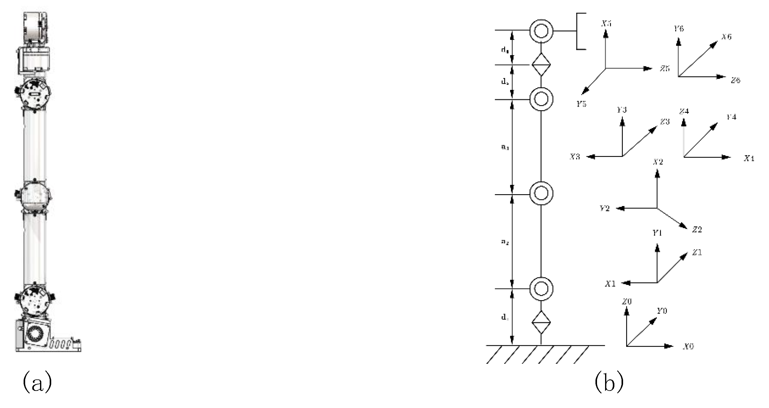
Robotic arms can only move within a defined spatial range due to the interrelated constraints and connections among their numerous joints. This limitation restricts the flexibility and diversity of motion, making it challenging for traditional path planning methods to adequately address the requirements of obstacle avoidance in manipulator path planning[24,25]. This study focuses on a six-degree-of-freedom robotic arm. The arm comprises six rotary joints of varying lengths that are connected in series, creating a modular structure. In this structure, the transformation matrix between two adjacent joints is first calculated, and the positional relationship from the base to the end effector is established through multiple matrix operations. Next, the standard Denavit-Hartenberg (D-H) model [26] is employed to establish the configuration of the coordinate system for each connecting rod. Specific D-H parameters are presented in Table 1.
As shown in Table 1, represents the linkage serial number;denotes the shortest distance between the two joint axes; indicates the clamp between the two linkages; represents the distance along the z-axis from the origin of thelinkage to the origin of the linkage; denotes the angle of rotation of the linkage, which is necessary for the linkage to align with the linkage; specifies the limit of the -joint.
Figure 2.
D-H Coordinate System of the Six-Degree-of-Freedom Manipulator: (a) 3D Model, (b) Structural Diagram of the Manipulator Arm and D-H Coordinate System.
Figure 2.
D-H Coordinate System of the Six-Degree-of-Freedom Manipulator: (a) 3D Model, (b) Structural Diagram of the Manipulator Arm and D-H Coordinate System.
Motion planning for robotic arms is a multi-body system problem that involves complex dynamics and geometry[27]. According to the algorithm proposed herein, the robotic arm can accurately navigate to a designated workspace location based on previously calculated position information of the singular value point. It can also determine the corresponding angular configurations of the joints at the singular value location, thereby enabling the robotic arm to move directly to the singular value point to perform a specific task or to avoid potential collisions. In the motion planning of a robotic arm, it involves the coordinated movement of multiple rigid structures. By applying the chi-square transformation matrix to each joint coordinate system, the position and orientation of each joint in the robotic arm are calculated. In article, the enhanced RRT* algorithm is employed to sample and plan the joint space of the manipulator. Collision detection is conducted on each of the generated joint poses to create an effective obstacle avoidance path.
2.2. Obstacle Collision Detection
In the manipulator’s workspace, there are both regular and irregular obstacles. The computational complexity of collision detection is high. To reduce computational complexity, the robot arm’s linkage can be abstracted as a cylinder. Therefore, it is essential to assess the potential collisions between each cylindrical feature of the manipulator and every obstacle in the environment. This paper employs the technique of enveloping the obstacle ball to streamline the handling of irregular obstacles. In this manner, the task of collision detection between the manipulator and the obstacle is converted into the problem of calculating the distance between a cylinder and a sphere. By equating the radius of a cylinder to the radius of a sphere, it is only necessary to calculate the distance between a straight line in space and the sphere. The schematic is presented in Figure 3. In addition, the article applies Obstacle Inflation for collision detection with standard obstacles. Consider the radius of a cylinder as the expansion dimension of a standard obstacle, also known as the safety margin. The collision detection between the manipulator and the obstacle is transformed into spatial straight-line collision detection, taking into account the expansion of the object[28]. The schematic diagram is shown in Figure 4.
2.2.1. Collision detection of irregular obstacles
In Figure 3a, represents the radius of the robotic arm linkage, denotes the radius of the obstacle envelope, and indicates the distance from the robotic arm linkage to the obstacle. In Figure 3b, the connecting rod of the manipulator is represented as a straight line in space, with its radius equal to that of the obstacle.
For the simplified obstacle collision detection model, it is necessary to calculate only the distance from the straight line to the center of the obstacle in space. The angles of each joint of the manipulator can be determined by solving the inverse kinematics for the desired end position and orientation. According to forward kinematics, the homogeneous transformation matrix for each link's coordinate system is derived. Therefore, the equivalent space linear equation of each link can be obtained. Because the base of the manipulator is fixed, only five links are required to determine whether the manipulator collides with obstacles. The distance r from the straight line to the center of the obstacle in space is calculated. If is less than or equal to the sum of the link radius and the obstacle envelope radius , a collision occurs; conversely, if is greater than this sum, no collision occurs.
2.2.2. Collision Detection of Regular Obstacles
In Figure 4a, represents the radius of the robotic arm linkage; indicates the distance from the robotic arm linkage to the obstacle. In Figure 4b, the linkage of the robotic arm is represented as a simplified spatial straight line . and are the starting and ending points of the linkage, respectively. The standard obstacle uses a cuboid as an example to expand the obstacle and create a larger boundary area, thereby simplifying collision detection. For each link segment, verify whether it intersects with the expanded area of the obstacle. If an intersection point exists, it can be concluded that the robotic arm will collide with the obstacle. If there is no intersection between the connecting rod segment and the obstacle, the minimum distance between the connecting rod segment and the line segment that forms the obstacle surface is calculated to assess the safe distance between the manipulator and the obstacle. The can be expressed as:
where is a point on the robotic arm linkage, denoted as ; is a point that represents the obstacle surface; denotes the Euclidean distance between points and .
Collision detection for square obstacles is accomplished by examining the intersection of the connecting rod with each face of the square. Each surface of the cube can be represented by a plane equation of the form: .a, b, and c are normal vectors to the plane, while is a constant term associated with the plane. The parameter for the intersection of the connecting rod with the square face can be expressed as:
If is within the range of [0, 1], the connecting rod intersects the surface and a collision occurs. Otherwise, no collision takes place.
2.3. Improved RRT* Based on Heuristic Probabilistic Sampling
2.3.1. Basics of the RRT*
The RRT* is a deterministic sampling-based path planning approach. It constructs a tree structure within the configuration space through an iterative process to identify the optimal path from the initial node to the target node . The principle of the RRT* is illustrated in Figure 5. In each iteration, the point is randomly sampled from the free space, and then the node with the minimum Euclidean distance to is selected from the tree. Based on this node, the step is extended in the direction of to generate a new node, . A tree node whose distance from is less than the sampling radius is identified from the tree to create a set . Then, the parent node is re-selected for in the set to minimize the path cost from the initial node to , and is inserted into the tree. After that, rewrite the nodes in , excluding the parent of . First, calculate the total cumulative cost of paths from to for all nodes. Then, evaluate whether designating as a parent node reduces the total cost of paths from to . If possible, update the parent of these nodes to . By means of continuous iteration, the RRT guarantees the asymptotic optimality of path cost, thereby facilitating efficient and robust path planning in complex environments.
2.3.2. Improved RRT* Based on Heuristic Probabilistic Sampling
In complex three-dimensional multi-obstacle environments, traditional RRT*encounter challenges related to inefficient search processes and excessive randomness in the selection of sampling points. So as to address the issue of reduced node sampling efficiency in three-dimensional multi-obstacle spaces, this study proposes an improved RRT* algorithm based on heuristic probabilistic sampling (HP-RRT*). The sampling process is optimized by generating a set of candidate nodes within a predefined sampling space and assessing the sampling priority of each candidate node through a specific heuristic function. By employing this method, it is possible to minimize redundant sampling nodes and enhance the efficiency of node sampling, thereby reducing the overall computation time.
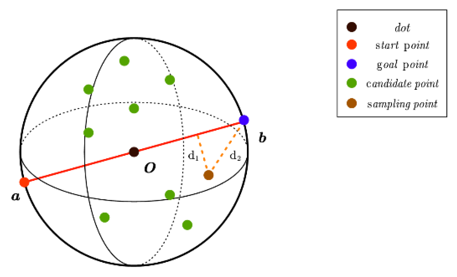
As illustrated in Figure 6, the starting point a and the endpoint b of the path are first connected. This line segment serves as the diameter to define a spherical space within which the sampling is conducted. Multiple candidate points are randomly generated in the spherical space as potential path nodes. The line segment connecting the starting point and the endpoint represents the shortest path.Give priority to the point nearest to the shortest path and the point closest to the endpoint. Design the corresponding heuristic function and calculate the weight value for each candidate point. Finally, the sampling probability for each candidate point is calculated and samples are drawn based on the corresponding weight values. The specific realization process is outlined as follows:
- Initialization phase;
Starting point: denoted by the symbol . It serves as the beginning of the search process and represents the starting position for all potential paths.
Goal Point: denoted by the symbol . It indicates the end point of the search process and serves as the destination for all paths.
Shortest path: In geometric path planning, the straight line segment connecting the start point and the end point is regarded as an approximation of the shortest path.
Sphere space: the sphere space is defined by the diameter of the line segment as the sampling region. The spherical space encompasses all possible path points, with boundaries defined by the endpoints of the line segment .
- 2.
- Candidate point generation;
Randomly generated point sets in spherical space are utilized as potential nodes in the search process for subsequent pathfinding. Points are generated based on a probability distribution, ensuring coverage of the entire search space and increasing the likelihood of discovering optimal paths.
- 3.
- Heuristic function design;
Heuristic function: provides a thorough assessment for estimating the cost of the shortest path from the current candidate point to the goal point. It considers both the distance from the candidate point to the shortest path and the distance from the candidate point to the goal point. It can be expressed as:
where denotes the candidate point; represents the distance from the candidate point to the line segment; identifies the radius of the sphere; controls the extent to which the distance from the shortest line segment influences the weight; expresses the distance from the candidate point to the goal point b; the extent to which the distance from point b affects the weight.
Figure 6.
Sampling space.
In order to more accurately capture the nonlinear relationship between weights and distance, a nonlinear function is employed instead of the traditional linear decay model, represented by the following expression.
where α and β are parameters that determine the decay rate.
To prevent numerical issues, establish a minimum value to ensure that the weights remain sufficiently large.
- 4.
- Sampling and path selection
The sampling probability for each candidate point is determined by Equation 7.
where represents the heuristic value of the candidate point, and denotes the total number of candidate points.
2.4. Improved HP-RRT* incorporating the APF
When path planning is conducted within the manipulator's workspace, it is inevitably influenced by obstacles, thereby increasing the complexity of the path planning process.
In order to solve this problem, based on the kinematic analysis of the robotic arm and employ the APF for path planning. This approach is integrated with the previously proposed highly efficient probabilistic sampling algorithm, HP-RRT*. In this algorithm, the potential field force of APF is utilized as an additional guiding force to influence the generation of sampling points and the selection of paths. This approach aims to enhance obstacle avoidance and results in a sub-optimal route that is close to the shortest path.
2.4.1. Traditional APF
The robotic arm obstacle avoidance model utilizing the APF algorithm is illustrated in Figure 7. The essence of the algorithm involves meticulously creating a virtual potential field within the workspace of the robotic arm and solving for it. The model is based on two primary potential fields: the target potential field and the obstacle potential field. The target point generates a global gravitational potential field at the end effector position of the manipulator, simulating an attractive force that encourages the manipulator to move toward the target point. On the contrary, the obstacle creates a localized repulsive potential field at the end effector position of the manipulator, simulating a repulsive force that helps the manipulator avoid collisions with the obstacle[29].
When the obstacle is outside the repulsive potential field, the end effector of the manipulator is influenced solely by the gravitational potential field and moves directly toward the target point. However, when the obstacle enters the repulsive potential field, the end of the manipulator is affected by both the repulsive potential field and the gravitational potential field. This superimposed effect of forces enables the robotic arm to dynamically plan a path for obstacle avoidance, effectively avoids obstacles and continues toward the target point.
In the spatial model of the APF, the target point is strategically identified as the lowest point in the potential field, specifically the minimum point of the potential function. By calculating the potential functions of the gravitational field and the repulsive field, and then superimposing them, one can obtain the potential function of the combined field. Under the influence of the combined potential field, the manipulator moves in the direction of the gradient descent of the potential function until it attains the target state.
The gravitational potential field is primarily associated with the distance between the end position of the robotic arm and the target point. As the distance increases, the value of the potential energy also increases; conversely, as the distance decreases, the value of the potential energy diminishes. The expression for the gravitational potential field is as follows.
where, is the gravitational potential field at the target point; is the positively proportional gain coefficient; denotes the current position of the robotic arm end-effector; indicates the desired position of the end-effector in the target configuration; vector function, the difference between the position vector of the robotic arm's end-effector, , and the ideal position of the target point, .
The corresponding gravitational force is the negative gradient of the gravitational field. It represents the fastest-changing direction of the gravitational potential field function . The expression is presented below.
The primary influence of the repulsive potential field is the distance between the robotic arm and the obstacle.The expression for the repulsive potential field is as follows:
where represents the repulsive potential field; is the positive proportionality gain coefficient; is a vector function, the difference between the position vector of the end-effector of the robotic arm, , and the obstacle, .
The repulsive potential field differs from the gravitational potential field in that the robotic arm is not always subjected to the repulsive force exerted by the barrier. When the relative distance between the manipulator and the obstacle exceeds , it is concluded that the obstacle does not affect the manipulator's operation. The smaller the relative distance between the arm and the obstacle, the greater the effect of the repulsive force and the higher the potential energy. Conversely, as the relative distance between the arm and the obstacle increases, the effect of the repulsive force diminishes, resulting in a decrease in potential energy.
The corresponding repulsive force is the negative gradient of the repulsive potential field. The expression can be represented as follows:
The magnitude of the robot's combined potential field is the sum of its repulsive and gravitational potential fields. Therefore, the expression for the total function of the combined potential field is:
The resultant force expression is :
Under the guidance of the virtual potential field, the robotic arm moves toward the direction of the steepest decrease in the combined potential field .This is typically where the final desired goal is situated.
In the application of the traditional APF, issues such as local minima and target unreachability arise[30]. Specifically, the trajectory of the robotic arm can be directed toward a region of force equilibrium, known as the Potential Well. As shown in Figure 8, the combined force acting on the robotic arm in this region approaches zero. In this state, the manipulator is prone to becoming trapped in a local minimum area, so it can not achieve the arrival of the target point. Due to the presence of a strong repulsive force field, the manipulator may display oscillatory behavior. This further hinders its ability to reach the intended target location and may ultimately result in the failure of the path planning task.
2.4.2. Improved APF
To address these issues, this paper presents an enhanced gravitational potential field function. This improved method adjusts to changes in distance between the manipulator and the target point, reduces the stagnation time of the manipulator within the potential well, and improves its ability to escape from local minima. The gravitational potential field can be expressed as:
where is the environmentally determined distance constant, and is the constant factor.
The corresponding expression for the gravitational force, , is presented in Equation 15.
The construction of the enhanced repulsive potential field is more complex than that of the attractive potential field. By adjusting the influence range and strength of the repulsive field function, the target unreachability can be mitigated, enabling the robotic arm to navigate around obstacles more effectively. The repulsive potential field can be expressed as:
where is the adjustment factor for the distance between the end actuator of the robotic arm and the target point, and represents the number of normals.
The corresponding repulsive force consists of two components: and . Their expressions are as follows:
where the first component of the repulsive force, directed from the obstacle to the end actuator position of the robotic arm; denotes the second component of the repulsive force, oriented from the end actuator position of the robotic arm toward the goal point.
2.4.3. HP-RRT* Incorporating APF
In the implementation of the HP-RRT* , this paper employs an optimized artificial potential field method to incorporate obstacle perception information. The algorithm captures real-time spatial distribution information of obstacles and calculates the potential field value for each candidate point to be integrated into the heuristic function. Selection of sampling points based on probabilistic algorithm. Although this improves the directionality of the sampling process and accelerates the convergence of the algorithm, it does not fundamentally alter the randomness of the new node generation process. In complex environments, this may cause the algorithm to become trapped in a local minimum and experience deviations due to repeated sampling, thereby reducing the efficiency of the path search. In order to solve this problem, the RRT* algorithm combining heuristic probability sampling with the APF, referred to as HP-APF-RRT* for short. It utilizes the superposition of the gravitational potential field function associated with the target point, and the repulsive potential field function related to the obstacle. This approach is applied to the neighboring nodes of the random tree algorithm . Thus, the growth of random tree nodes is influenced not only by the gravitational potential field function of the sampling point but also by the combined effects of target attraction and obstacle repulsion. Figure 9 illustrates the impact of the artificial potential field method on the expansion of random tree nodes.
The expressions for the gravitational potential field and the gravitational force calculated for the neighboring node in the tree, with respect to the sampling point, are as follows:
The total potential field value is defined as the difference between the gravitational potential field and the repulsive potential field, expressed as:
The expression for the heuristic function is denoted as:
where denotes the weighting factor used to balance the impact of on the total cost.
In the implementation process of the entire algorithm, weighted sampling in the sphere function is utilized to calculate the probability distribution, allowing for the random generation of the sampling point in the configuration space. Subsequently, FindNearestPoint function is used to identify the node that is closest to within the path planning tree. Next, the geometric angle between and 、, and the set of obstacles is computed using compute_angle function. Based on the known angle , the gravitational components and of , , and in the,and axis directions, respectively, are calculated using compute_Attract function. At the same time, the repulsive force component of each obstacle relative to the nearest point is calculated in the , , and axis directions, taking into account the compute repulsion and the angle .The combined force is determined by integrating the gravitational and repulsive components using the following expression:
The combined force determines the search direction, , according to the following expression:
The new node position, , is calculated using Equation 26.
Perform collision detection on and add it to the path planning tree if no collisions are detected. Iterate until the algorithm's termination condition is met, ultimately generating an optimal path from the starting point to the target point. The general process of the algorithm is shown in Figure 10.
2.5. Path Optimization Based on Trigonometric Inequalities
In three-dimensional space, pathfinding using the RRT* and its derivative algorithms produces a continuous line segment composed of a series of discrete points. However, this process frequently generates a significant number of redundant nodes. The presence of these nodes hinders the smooth operation of the robotic arm[31].
In this text, the triangle inequality is used to optimize each node in the path. Node cost evaluation is essential for parent node reselection, rewriting, and path optimization algorithms. Eq. 27 is used to evaluate the trade-offs associated with node expansion by integrating path cost, security cost, and stability cost.
where represents the cumulative path cost from the starting point to the current node ; signifies the security cost, is the reciprocal of the average distance between the current node c and its neighboring obstacles; is the stability cost, which reflects the path depletion from the parent node to the current node ; serve as weighting factors that correspond to the respective sub-costs within the total cost calculation.
After obtaining the initial path, it undergoes further optimization. Refer to Figure 11 for a schematic representation of the optimization process. If the grandfather node of node C is used as its parent node, the cost can be reduced without causing a collision, meaning that the triangle inequality is satisfied. The parent node of node C is updated to its grandparent node. On the contrary, if the grandparent node of node C collides with node C, it is considered that both node C and its parent node have been optimized. This process is carried out recursively until the initial node is transformed into the node to be optimized, thereby completing the entire optimization process.
3. Experiments and Analysis
This section aims to experimentally validate the performance of the HP-APF-RRT*. For this reason, this study compares and analyzes the improved HP-APF-RRT* with the existing RRT, RRT*, P-RRT*, and the HP-RRT* proposed in this paper, all within a unified three-dimensional simulation environment. The goal is to verify the superiority, validity, and reliability of the improved HP-APF-RRT* in path planning.
The simulation experiments are conducted on a Windows 10 operating system platform equipped with an Intel Core i5-12490F processor (with a base frequency of 3.0 GHz) and 16 GB of RAM. An efficient, collision-free path from the initial point to the target point is successfully planned. In addition, this study also uses the NZ500-500 model manipulator from Jizhi Technology Co., Ltd.for simulation and physical experiments to further validate the practical application potential of the algorithm.
3.1. Simulation Experiment Analysis
In order to thoroughly assess the superiority of the algorithm proposed in this paper compared to existing algorithms, this study conducts comparative experiments within a fixed and challenging 3D spatial environment. All algorithms were tested through simulations in two intricately designed 3D spatial environments.
In the experimental setup, the total area of the manipulable space for the robotic arm was established to be 1000 mm × 1000 mm. The gray areas on the map delineate the boundaries of the mobile space, and the cylinders, rectangles, and spheres within the map represent various types of static obstacles. The experimental parameters are set as follows: the general step size (step) is set to 10 mm, the number of candidate points (num_candidates) is 10, the gravitational gain coefficient of the target point (k) is set to 1.5, the gravitational gain coefficient of the sampling point (s) is set to 1, the repulsive gain coefficient of the obstacle is set to 1, the distance of obstacle influence (po) is set to 100 mm, and the maximum number of iterations (max_iterations) is set to 10,000.
In Scene 1, the coordinates of the red starting point coordinates are (100,100,100) mm and the blue target point are (900, 900, 900) mm. The results of the algorithm's planning are detailed in Figure 12. Each set of experiments was conducted 200 times to ensure the statistical significance of the results, and the mean data from the experiments are summarized in Table 2. Figure 12a–e show the path diagrams generated by various algorithms. Among them, the blue line illustrates the exploration tree structure of the algorithm, and the red solid line denotes the path planned by the corresponding algorithm. In order to reflect the boundary-extension property of the algorithm, no additional safety distances were incorporated into the actual collision judgment. As a result, the path lines appear to be very close to the surface of the obstacle.
The experimental results indicate that the average search time of the HP-APF-RRT* is the shortest, at only 1.039 seconds, which is significantly lower than that of the other algorithms. The average number of node samples generated by the algorithm is 2,290, which is significantly lower than that of other algorithms. This indicates that the HP-APF-RRT* has clear advantages in sampling efficiency. In terms of path optimization, the average path length of the HP-APF-RRT* is 1,461.463, which is the shortest among all the algorithms, demonstrating its high efficiency in path optimization. Meanwhile, the HP-APF-RRT* demonstrates a search success rate of 100% and successfully completes the planning task in all tests, highlighting its robustness in complex environments.
In contrast, the traditional RRT exhibits the longest path length and a search success rate of only 91%. Although it has a shorter average search time, this indicates deficiencies in both path optimization and robustness.
The RRT* and P-RRT*, although asymptotically optimal, do not demonstrate significant differences in average path lengths. Additionally, there are instances of planning failures, with search success rates of 93% for both algorithms.
The HP-RRT* and the HP-APF-RRT* utilize a heuristic sampling strategy, which offers significant advantages in terms of average search time, the number of sampled nodes, and path length. The HP-APF-RRT, which incorporates the APF, demonstrates increased sensitivity to obstacle perception. This enhancement effectively directs the sampling points to circumvent obstacles, thereby reducing the number of sampling points required.
In Scene 2, the narrative is more complex than in Scene 1. The basic settings remain consistent with those in Scene 1. The coordinates of the red starting point are (100, 100, 100) mm, while the coordinates of the blue target point are (900, 900, 500) mm. The results of the algorithm's planning are detailed in Figure. 13. Each set of experiments was conducted 200 times, and the average data from these experiments are summarized in Table 3. Figure 13a–e illustrate the path diagrams produced by various algorithms.
The results of this experiment are similar to scenario one. The HP-APF-RRT* excels in several key performance metrics, particularly in search time, sampling efficiency, path length, and search success rate.
Finally, after optimizing the path in accordance with the triangular inequality, the optimization results presented in Table 4 have been obtained. The optimized path is shown in Figure 14.
The optimization results indicate that the average path length has been improved from 1467.493 to 1461.463 in Scenario I and from 1286.505 to 1275.741 in Scenario II. These data show that the optimized path length is reduced, further verifies the algorithm's effectiveness in path optimization.
Through the experimental analysis of Scenario 1 and Scenario 2, the HP-APF-RRT* proposed in this paper demonstrates superior performance in complex environments with multiple obstacles.In both scenarios, despite differing complexities, the HP-APF-RRT* achieves the shortest search time and the fewest number of node samples. It also provides the optimal path length and maintains a 100% search success rate. These results confirm that the HP-APF-RRT surpasses other algorithms in search efficiency, node sampling efficiency, path optimization, and robustness, demonstrating its effectiveness and practicality in addressing complex path planning challenges.
3.2. Physical Experiment Analysis
In order to assess the effectiveness of the HP-APF-RRT* proposed in text for practical applications, an experimental environment was established within the framework of the Robot Operating System (ROS) using the NZ500-500 model robotic arm from Machine Technology Co. The initial step of the experiment was to construct a complex environmental scenario containing static obstacles, initial configuration points, and target configuration points within the Gazebo simulation software. In the ROS environment, the NZ500-500 manipulator model were loaded and visualized in three dimensions using the Gazebo tool. The HP-APF-RRT* directs the robotic arm using the MoveIt motion planning framework to facilitate obstacle avoidance. Ultimately, it successfully devises a collision-free path that satisfies the specified requirements.
As shown in Figure 15, key elements within the experimental scenarios have been designated with specific specialized symbols. The red square represents the target to be grasped, specifically the entity to be recognized and manipulated by the robotic arm. The purple columns symbolize the static obstacles in the path planning, which serve as physical barriers along the trajectory from the starting point to the endpoint. The black table represents the placement area, which is the final destination of the robotic arm's operation and signifies the completion stage of the task .
Figure 15 illustrates the four key positions of the NZ500-500 robotic arm as it executes the path planning task from the starting point to the target point: the initial position, the gripping position, the intermediate position during movement, and the target position.
Real-time control of the NZ500-500 robotic arm and its interaction with the environment are achieved through the integration of the MoveIt motion planning framework with the ROS. Under this framework, the various key poses involved in the obstacle avoidance experiment of the robotic arm—including the initial, grasping, intermediate, and target poses—are precisely synchronized and scheduled using the topics and services of ROS. These intricate motion sequences and positional transformation processes are illustrated in Figure 16.
In order to verify the feasibility and superiority of the algorithm through real experiments, Under the same obstacle conditions described above, twenty simulations were conducted for each algorithm, and the results were averaged, as shown in Table 5.
The experimental data demonstrate that the HP-APF-RRT* exhibits high efficiency in motion planning during simulation experiments. This efficiency is evident in the algorithm's optimality and completeness, specifically in its ability to determine the shortest paths and facilitate the fastest planning. The HP-APF-RRT* algorithm also performs well in physical experiments incorporating real-world application scenarios. Its performance satisfies the motion requirements of a real robotic arm, particularly in the time needed to execute the gripping action, which is shorter than that of other algorithms.
4. Conclusions
In study, a six-degree-of-freedom robotic arm is selected as the research subject. The standard D-H parameter model is employed to establish its coordinate system and to derive both its forward and inverse kinematic equations. On this basis, an improved RRT * path planning algorithm ( HP-APF-RRT*) combining heuristic probability sampling strategy with the artificial potential field method. This approach aims to address the issues of low sampling efficiency, extended computation time, non-optimal paths, and failures in pathfinding within complex environments that are encountered by the traditional RRT* in three-dimensional space path planning.The algorithm minimizes redundant sampling nodes and enhances sampling efficiency by incorporating heuristic probabilistic sampling techniques. At the same time, the artificial potential field method is introduced to construct gravitational and repulsive fields. This approach guides the sampling points to avoid obstacles and move toward the target point, enhances the gravitational effect on the sampling points, and adjusts the direction of node extension. This method effectively addresses the pathfinding problem in complex environments. In addition, redundant intermediate nodes are streamlined using triangular inequalities to further optimize the path.
The results of the experimental simulation confirm the superiority of the algorithm compared to traditional algorithms, particularly in multi-obstacle sampling environments. Physical experiments further validate the feasibility of the algorithm in practical applications. Compared to the traditional RRT* algorithm, the running speed of this algorithm has been significantly enhanced.
The work presented in this paper has significant potential for improvement. Real-time path planning for dynamic target points is a significant research challenge, particularly in the context of utilizing reinforcement learning algorithms for moving target points. In real-world applications, such as robotic arm garbage sorting, real-time target tracking, and dynamic target path planning, traditional path planning algorithms must be integrated with reinforcement learning. This combination enhances adaptability and robustness in response to dynamically changing environments.
Author Contributions
Conceptualization, X.Z.; methodology, X.Z. and P.W.; software, X.Z. and P.W.; validation, P.W.; formal analysis, Y.G. and Q.H.;investigation, K.Z. and P.W.; resources, X.Z.; data curation, P.W.;writing—original draft preparation, X.Z. and P.W.; writing—review and editing,X.Z. and P.W.; visualization, Y.G. and Q.H.; supervision, K.Z. project administration, X.Z. and P.W.; funding acquisition, X.Z. All authors have read and agreed to the published version of the manuscript.
Funding
This research was funded by the Shanxi Province Basic Research Program, grant number 202203021221160 and Intelligent Transportation Shanxi Laboratory Open Fund, grant number 2024-ITLOP-KD-01.
Institutional Review Board Statement
Not applicable.
Informed Consent Statement
Not applicable.
Data Availability Statement
The data presented in this study are available on request from the corresponding author.
Conflicts of Interest
The authors declare no conflict of interest.
References
- Husainy, A.; Mangave, S.; Patil, N. J. A. R. o. M. E., A Review on Robotics and Automation in the 21st Century: Shaping the Future of Manufacturing, Healthcare, and Service Sectors. 2023, 12 (2), 41-45. [CrossRef]
- Dong, L.; He, Z.; Song, C.; Sun, C. J. J. o. S. E.; Electronics, A review of mobile robot motion planning methods: from classical motion planning workflows to reinforcement learning-based architectures. 2023, 34 (2), 439-459. [CrossRef]
- Kang, H. I.; Lee, B.; Kim, K. In Path planning algorithm using the particle swarm optimization and the improved Dijkstra algorithm, 2008 IEEE Pacific-Asia Workshop on Computational Intelligence and Industrial Application, IEEE: 2008; pp 1002-1004.
- Han, C.; Li, B. In Mobile robot path planning based on improved A* algorithm, 2023 IEEE 11th Joint International Information Technology and Artificial Intelligence Conference (ITAIC), IEEE: 2023; pp 672-676.
- Li, B.; Chen, B. J. I. C. J. o. A. S., An adaptive rapidly-exploring random tree. 2021, 9 (2), 283-294. [CrossRef]
- Li, Q.; Xu, Y.; Bu, S.; Yang, J. J. S., Smart vehicle path planning based on modified PRM algorithm. 2022, 22 (17), 6581. [CrossRef]
- Li, Y.; Wei, W.; Gao, Y.; Wang, D.; Fan, Z. J. E. s. w. a., PQ-RRT*: An improved path planning algorithm for mobile robots. 2020, 152, 113425. [CrossRef]
- Liu, H.; Zhang, S.; Yang, X. J. R. P. o. E., Overview of Path Planning Algorithms. 2024, 18 (7), 76-89. [CrossRef]
- Liu, J.; Yap, H. J.; Khairuddin, A. S. M. J. J. o. S., Review on Motion Planning of Robotic Manipulator in Dynamic Environments. 2024, 2024 (1), 5969512. [CrossRef]
- Liu, L.; Wang, X.; Yang, X.; Liu, H.; Li, J.; Wang, P. J. E. S. w. A., Path planning techniques for mobile robots: Review and prospect. 2023, 227, 120254. [CrossRef]
- Sotirchos, G.; Ajanovic, Z. J. a. p. a., Search-based versus Sampling-based Robot Motion Planning: A Comparative Study. 2024.
- Karaman, S.; Frazzoli, E. J. T. I. J. o. R. R., Sampling-based algorithms for optimal motion planning. 2011, 30, 846 - 894.
- Qi, J.; Yuan, Q.; Wang, C.; Du, X.; Du, F.; Ren, A. J. C.; Systems, I., Path planning and collision avoidance based on the RRT* FN framework for a robotic manipulator in various scenarios. 2023, 9 (6), 7475-7494. [CrossRef]
- LaValle, S. M.; Kuffner, J. J. J. T. I. J. o. R. R., Randomized Kinodynamic Planning. 1999, 20, 378 - 400. [CrossRef]
- Zhou, Y.; Huang, N. J. S. C. I.; Systems, Airport AGV path optimization model based on ant colony algorithm to optimize Dijkstra algorithm in urban systems. 2022, 35, 100716. [CrossRef]
- Yi, J.; Yuan, Q.; Sun, R.; Bai, H. J. C.; systems, i., Path planning of a manipulator based on an improved P_RRT* algorithm. 2022, 8 (3), 2227-2245. [CrossRef]
- Tao, F.; Ding, Z.; Fu, Z.; Li, M.; Ji, B. J. S. R., Efficient path planning for autonomous vehicles based on RRT* with variable probability strategy and artificial potential field approach. 2024, 14. [CrossRef]
- Wang, J.; Li, T.; Li, B.; Meng, M. Q.-H. J. I. T. o. I. V., GMR-RRT*: Sampling-based path planning using gaussian mixture regression. 2022, 7 (3), 690-700. [CrossRef]
- Wang, J.; Chi, W.; Li, C.; Wang, C.; Meng, M. Q.-H. J. I. T. o. A. S.; Engineering, Neural RRT*: Learning-based optimal path planning. 2020, 17 (4), 1748-1758. [CrossRef]
- Chai, Q.; Wang, Y. J. A. S., RJ-RRT: improved RRT for path planning in narrow passages. 2022, 12 (23), 12033. [CrossRef]
- Luders, B.; Kothari, M.; How, J. In Chance constrained RRT for probabilistic robustness to environmental uncertainty, AIAA guidance, navigation, and control conference, 2010; p 8160.
- Zhang, W.; Xu, G.; Song, Y.; Wang, Y. J. J. o. F. R., An obstacle avoidance strategy for complex obstacles based on artificial potential field method. 2023, 40 (5), 1231-1244. [CrossRef]
- Mall, K.; Grant, M. J.; Taheri, E. J. J. o. S.; Rockets, Uniform trigonometrization method for optimal control problems with control and state constraints. 2020, 57 (5), 995-1007. [CrossRef]
- Stilman, M. J. I. T. o. R., Global manipulation planning in robot joint space with task constraints. 2010, 26 (3), 576-584. [CrossRef]
- Stilman, M. In Task constrained motion planning in robot joint space, 2007 IEEE/RSJ International Conference on Intelligent Robots and Systems, IEEE: 2007; pp 3074-3081.
- Lee, J.-W.; Park, G.-T.; Shin, J.-S.; Woo, J.-W. In Industrial robot calibration method using denavit—Hatenberg parameters, 2017 17th International Conference on Control, Automation and Systems (ICCAS), IEEE: 2017; pp 1834-1837.
- Dai, Y.; Xiang, C.; Zhang, Y.; Jiang, Y.; Qu, W.; Zhang, Q. J. A., A review of spatial robotic arm trajectory planning. 2022, 9 (7), 361. [CrossRef]
- Zhuang, M.; Li, G.; Ding, K. J. I. A., Obstacle avoidance path planning for apple picking robotic arm incorporating artificial potential field and a* algorithm. 2023.
- Cheng, X.; Zhou, J.; Zhou, Z.; Zhao, X.; Gao, J.; Qiao, T. J. J. o. I. I. I., An improved RRT-Connect path planning algorithm of robotic arm for automatic sampling of exhaust emission detection in Industry 4.0. 2023, 33, 100436. [CrossRef]
- Gao, Q.; Yuan, Q.; Sun, Y.; Xu, L. J. J. o. K. S. U.-C.; Sciences, I., Path planning algorithm of robot arm based on improved RRT* and BP neural network algorithm. 2023, 35 (8), 101650. [CrossRef]
- Agirrebeitia, J.; Avilés, R.; De Bustos, I. F.; Ajuria, G. J. M.; Theory, M., A new APF strategy for path planning in environments with obstacles. 2005, 40 (6), 645-658. [CrossRef]
Figure 3.
Collision Detection Model of a Robotic Arm with Irregular Obstacles: (a) Original Collision Model; (b) Simplified Collision Model.
Figure 3.
Collision Detection Model of a Robotic Arm with Irregular Obstacles: (a) Original Collision Model; (b) Simplified Collision Model.
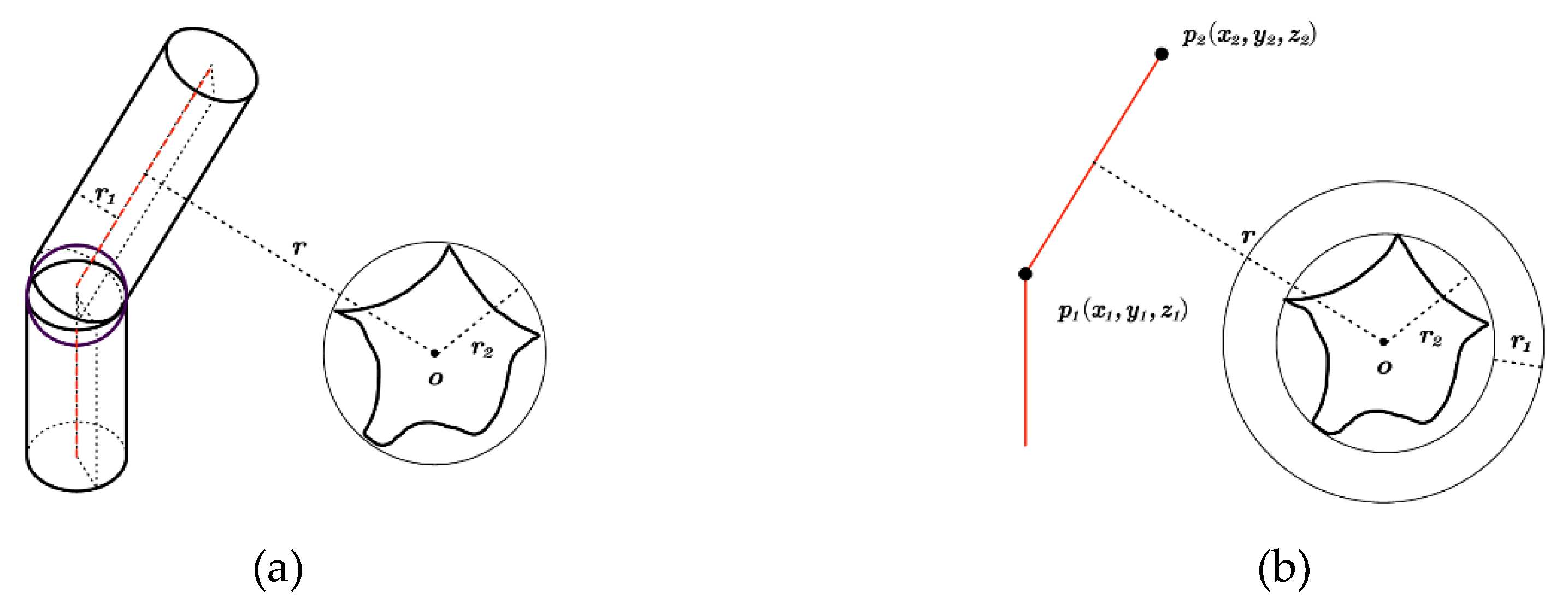
Figure 4.
Collision Detection Model of a Robotic Arm with Regular Obstacles: (a) Original Collision Model; (b) Simplified Collision Model.
Figure 4.
Collision Detection Model of a Robotic Arm with Regular Obstacles: (a) Original Collision Model; (b) Simplified Collision Model.
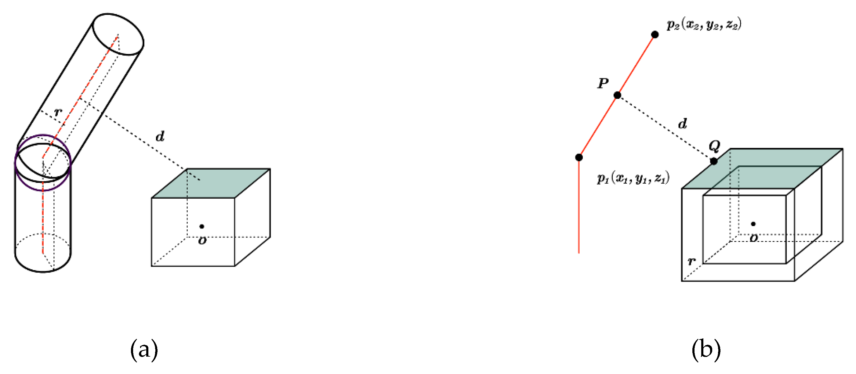
Figure 5.
RRT* algorithm flow.
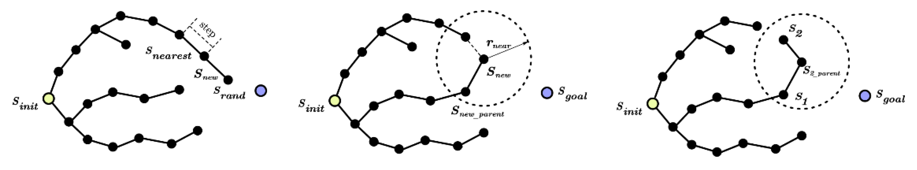
Figure 7.
Robotic arm obstacle avoidance model of APF algorithm.
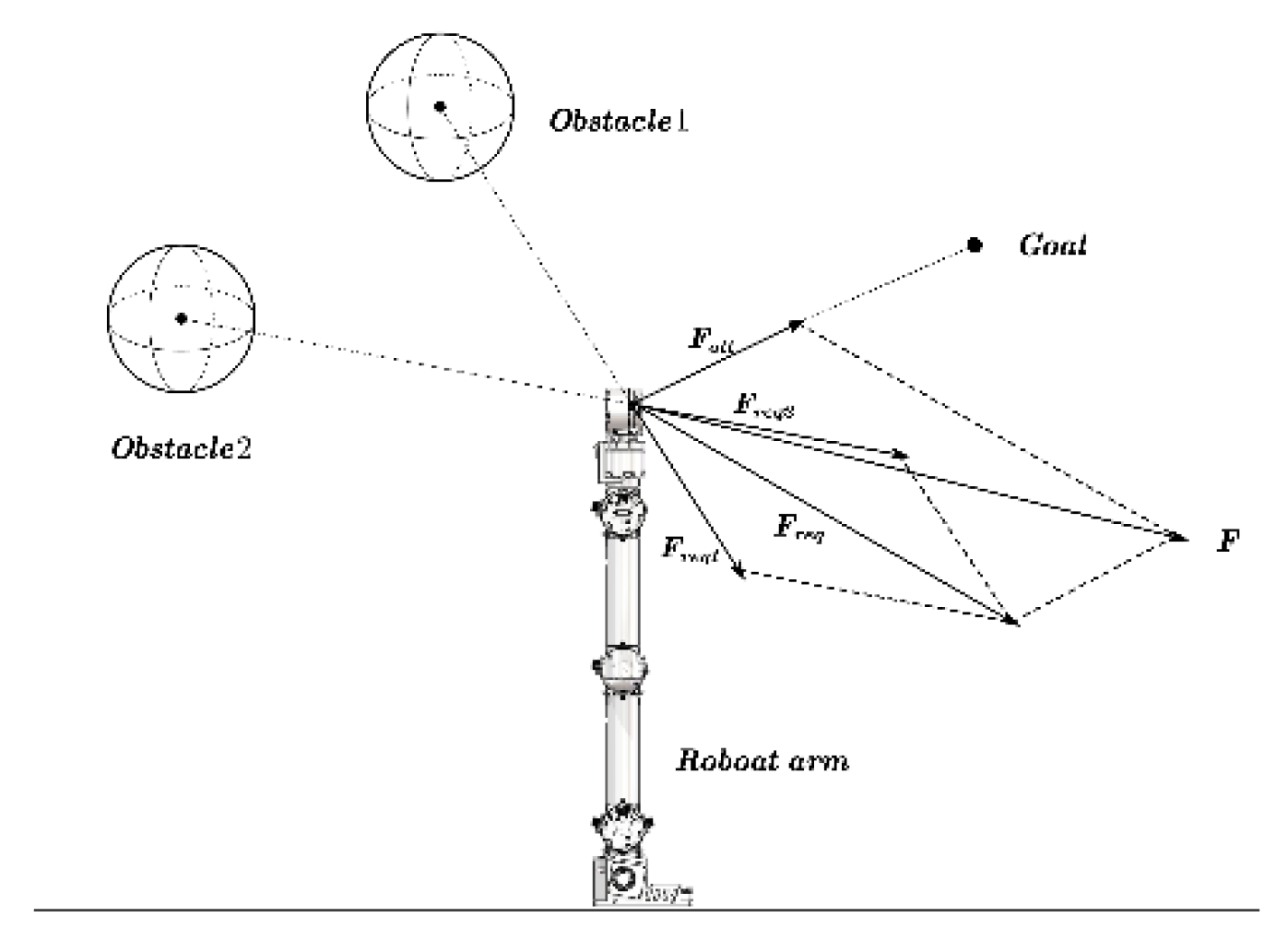
Figure 8.
Potential well problem.
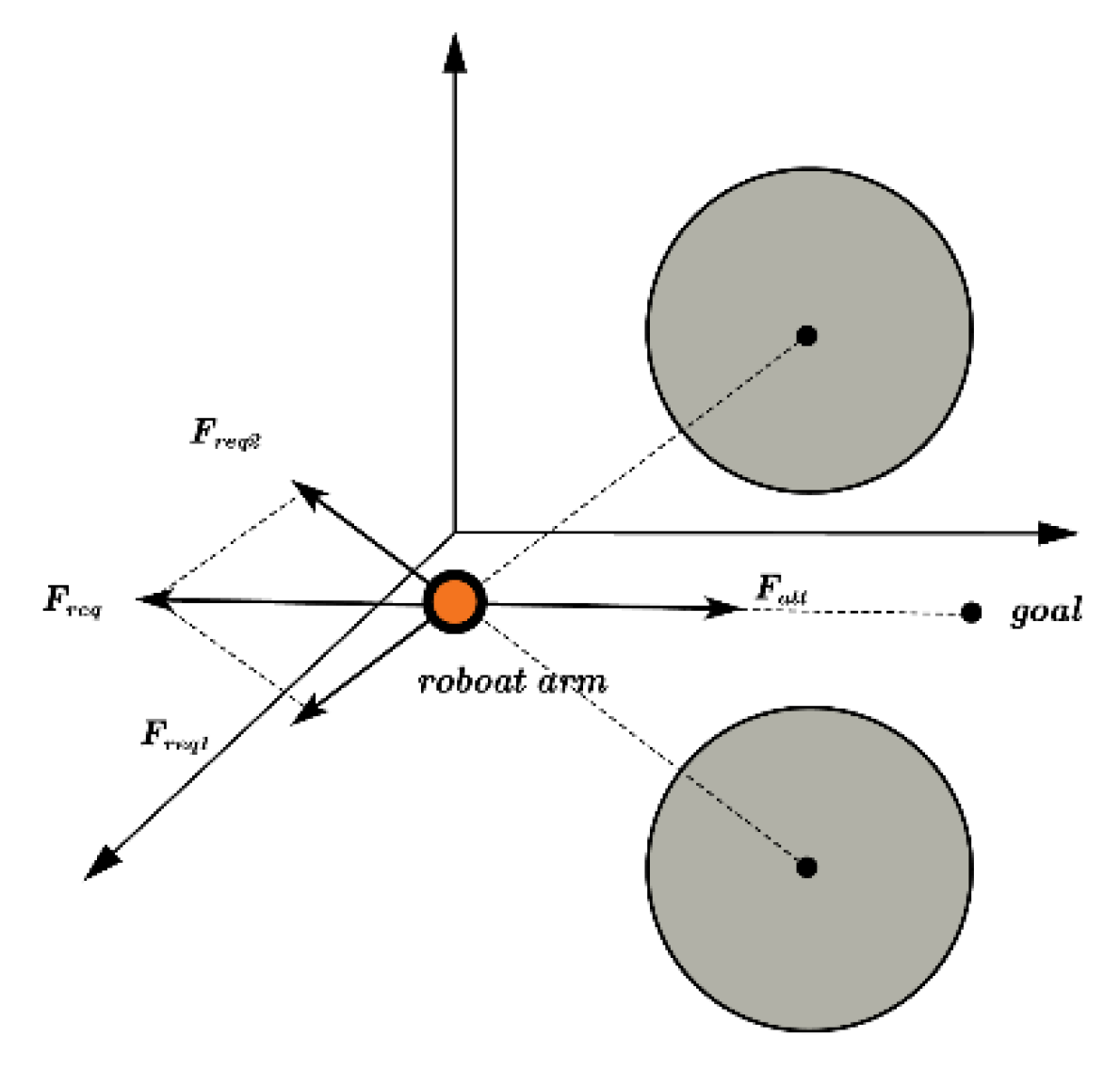
Figure 9.
Schematic diagram of the algorithm.
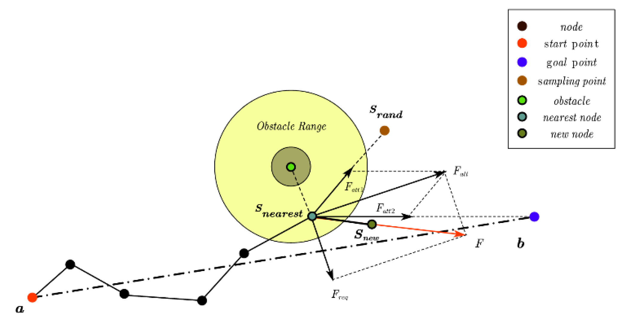
Figure 10.
Flowchart of the algorithm.
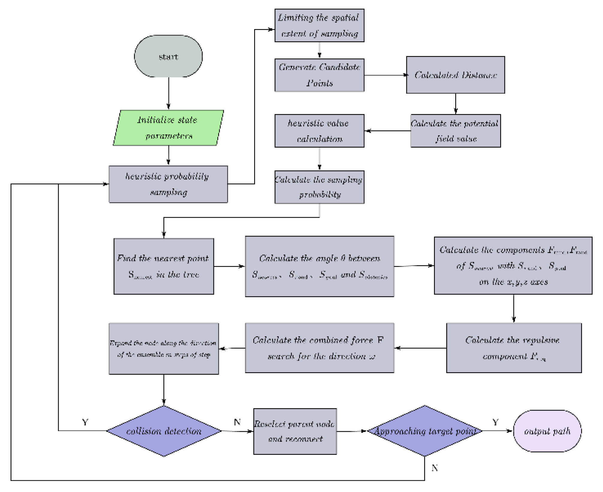
Figure 11.
Path optimization.
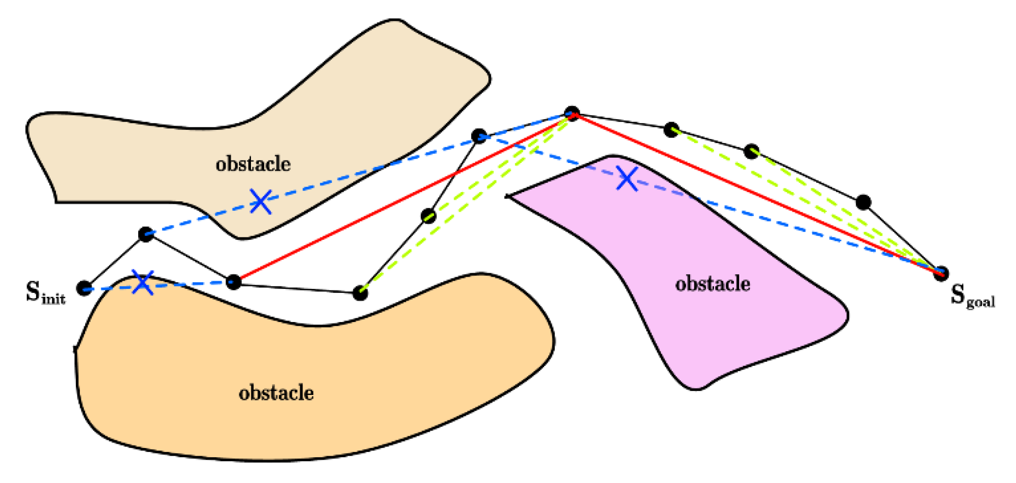
Figure 12.
Different algorithms to generate paths in scenario I: (a) RRT; (b) RRT*; (c) P-RRT*; (d) HP-RRT*; (e) HP-APF-RRT*.
Figure 12.
Different algorithms to generate paths in scenario I: (a) RRT; (b) RRT*; (c) P-RRT*; (d) HP-RRT*; (e) HP-APF-RRT*.
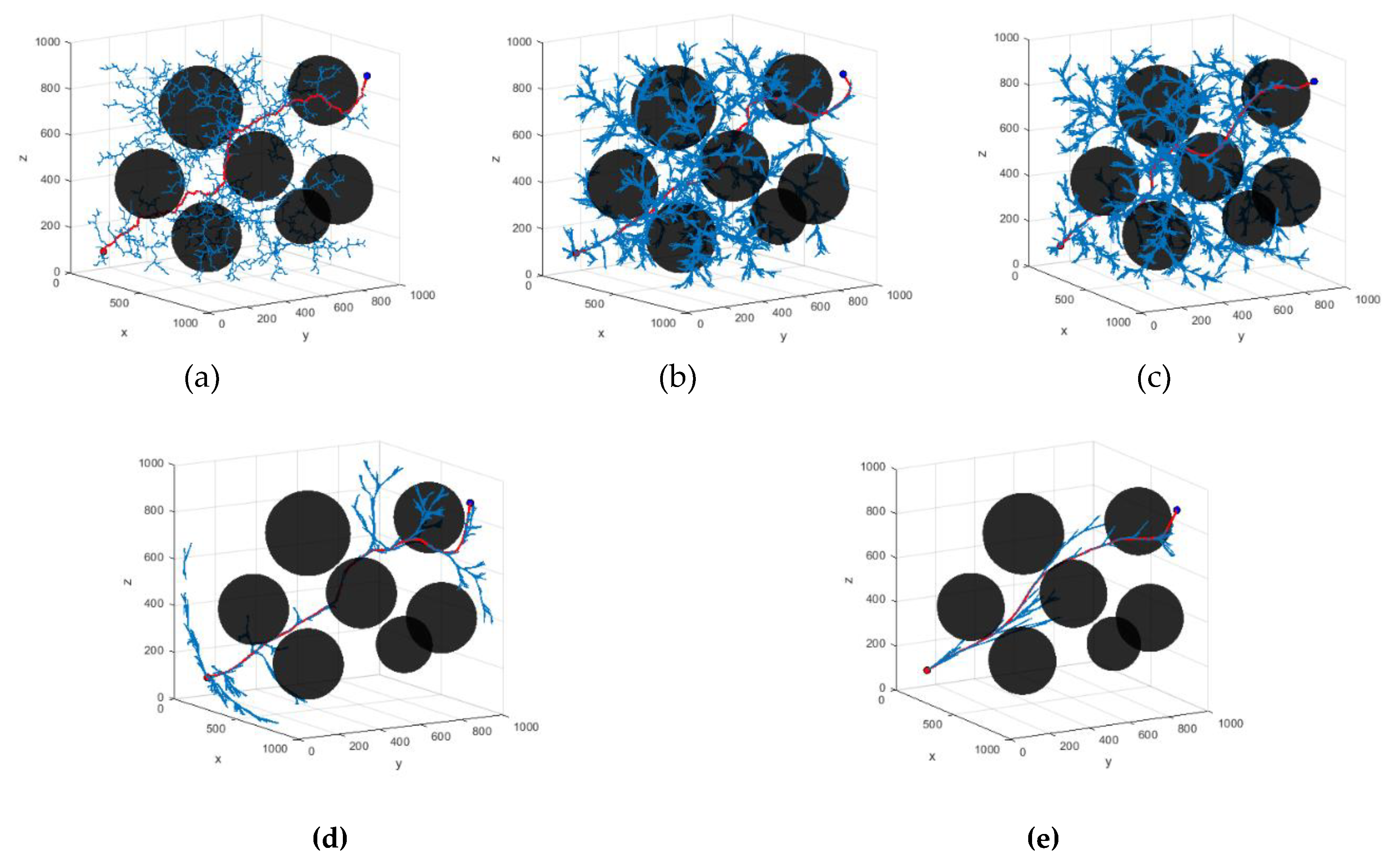
Figure 13.
Different algorithms to generate paths in scenario II: (a) RRT; (b) RRT*; (c) P-RRT*; (d) HP-RRT*; (e) HP-APF-RRT*.
Figure 13.
Different algorithms to generate paths in scenario II: (a) RRT; (b) RRT*; (c) P-RRT*; (d) HP-RRT*; (e) HP-APF-RRT*.
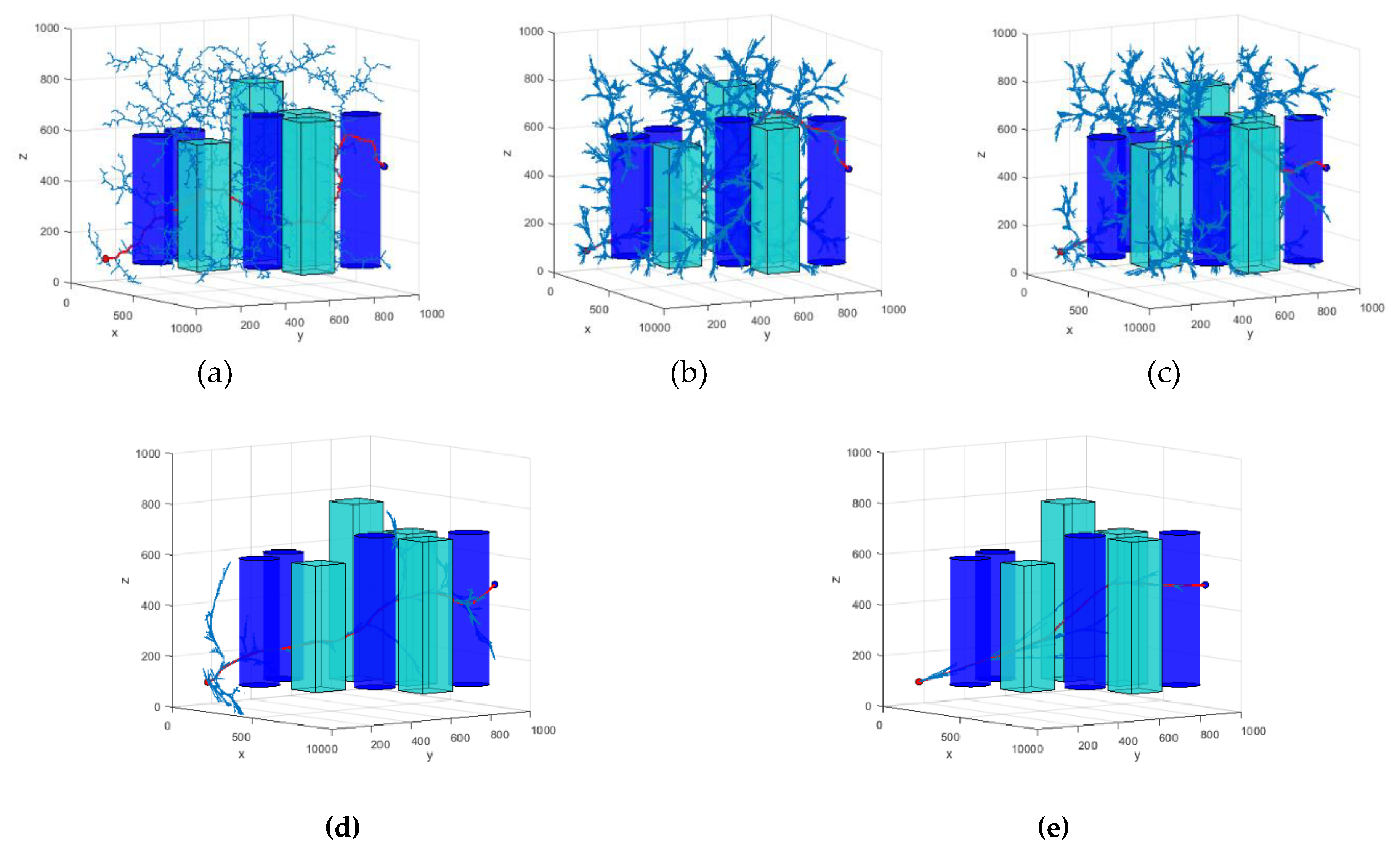
Figure 14.
Comparison of optimization algorithms: (a) Scenario 1 unoptimized path; (b) Scenario 1 optimized path; (c) Scenario 2 unoptimized path; (d) Scenario 2 optimized path.
Figure 14.
Comparison of optimization algorithms: (a) Scenario 1 unoptimized path; (b) Scenario 1 optimized path; (c) Scenario 2 unoptimized path; (d) Scenario 2 optimized path.
Figure 15.
Robotic arm poses: (a) initial pose; (b) gripping pose; (c) intermediate pose; (d) target pose.
Figure 15.
Robotic arm poses: (a) initial pose; (b) gripping pose; (c) intermediate pose; (d) target pose.
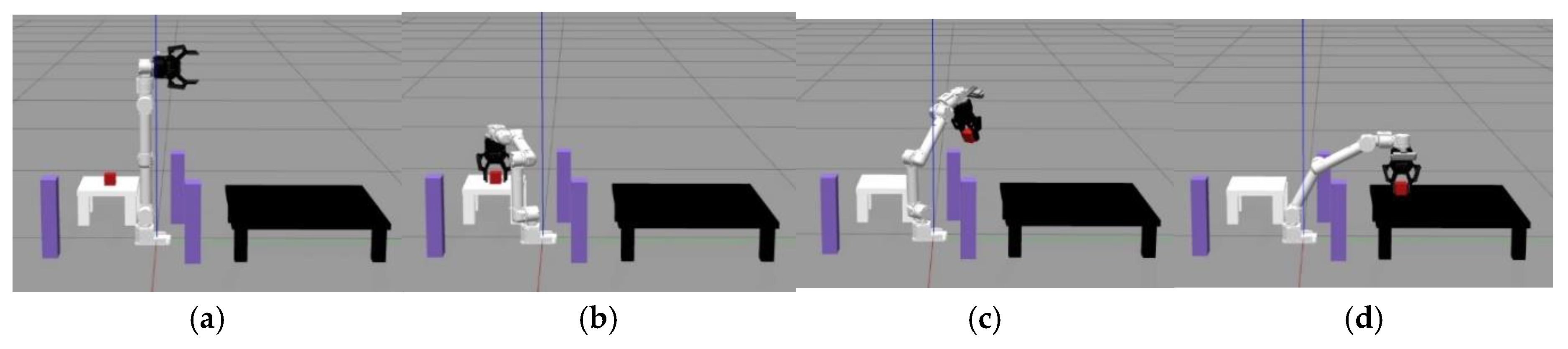
Figure 16.
Real robotic arm poses: (a) initial pose; (b) gripping pose; (c) intermediate pose; (d) target pose.
Figure 16.
Real robotic arm poses: (a) initial pose; (b) gripping pose; (c) intermediate pose; (d) target pose.
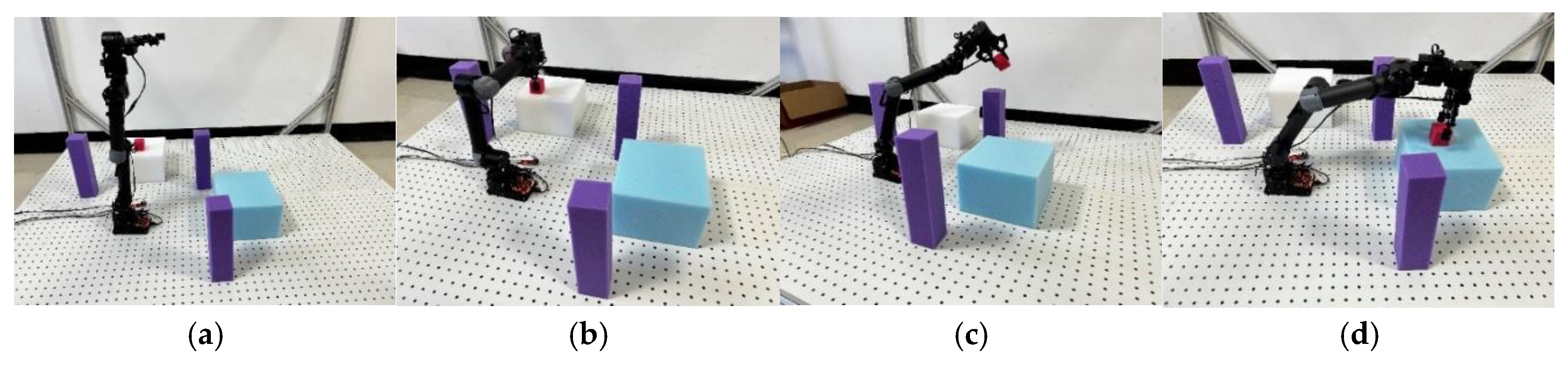

Table 1.
Standard D-H parameters of six degrees of freedom anipulator.
| Connect rod serial number(i) | /mm | /(°) | /mm | (°) | (°) |
|---|---|---|---|---|---|
| 1 | 0 | -90 | 92.5 | ± 180 | |
| 2 | 189 | 90 | 0 | ± 135 | |
| 3 | 189 | -90 | 0 | ± 150 | |
| 4 | 0 | 0 | 0 | -170~+180 | |
| 5 | 0 | -90 | 36 | ± 120 | |
| 6 | 0 | 0 | 86 | ± 360 |
Table 2.
Comparison of Scene 1 algorithms
| Algorithm name | Average search time/s | Average number of node samples | Average path length | Search Success Rate |
|---|---|---|---|---|
| RRT | 4.203 | 5703 | 2112.441 | 91% |
| RRT* | 7.262 | 5513 | 1686.495 | 93% |
| P-RRT* | 7.768 | 5539 | 1690.284 | 93% |
| HP-RRT* | 3.015 | 2544 | 1713.812 | 100% |
| HP-APF-RRT* | 1.039 | 2290 | 1467.493 | 100% |
Table 3.
Comparison of Scene 2 algorithms
| Algorithm name | Average search time/s | Average number of node samples | Average path length | Search Success Rate |
|---|---|---|---|---|
| RRT | 4.625 | 6304 | 1935.640 | 73% |
| RRT* | 10.415 | 6297 | 1530.290 | 61% |
| P-RRT* | 11.925 | 6488 | 1549.293 | 67% |
| HP-RRT* | 2.237 | 1978 | 1445.297 | 100% |
| HP-APF-RRT* | 0.889 | 1576 | 1286.505 | 100% |
Table 4.
Comparison of optimization algorithms.
| Algorithm name | Average path length | Average optimized path length |
|---|---|---|
| scenario one | 1467.493 | 1461.463 |
| scenario two | 1286.505 | 1275.741 |
Table 5.
Comparison of algorithms.
| Algorithm name | Average grasp time/s | Average search time/s | Search Success Rate |
| RRT | 49.65 | 24.75 | 85% |
| RRT* | 58.74 | 36.71 | 80% |
| P-RRT* | 53.61 | 32.95 | 85% |
| HP-RRT* | 24.85 | 7.56 | 100% |
| HP-APF-RRT* | 19.79 | 5.62 | 100% |
Disclaimer/Publisher’s Note: The statements, opinions and data contained in all publications are solely those of the individual author(s) and contributor(s) and not of MDPI and/or the editor(s). MDPI and/or the editor(s) disclaim responsibility for any injury to people or property resulting from any ideas, methods, instructions or products referred to in the content. |
© 2024 by the authors. Licensee MDPI, Basel, Switzerland. This article is an open access article distributed under the terms and conditions of the Creative Commons Attribution (CC BY) license (http://creativecommons.org/licenses/by/4.0/).
Copyright: This open access article is published under a Creative Commons CC BY 4.0 license, which permit the free download, distribution, and reuse, provided that the author and preprint are cited in any reuse.


