
Submitted:
11 March 2025
Posted:
13 March 2025
You are already at the latest version
Abstract
This study presents the kinematic synthesis of planar mechanisms using precision point analysis for three, four, and five target positions. The research explores the application of graphical synthesis techniques to design mechanisms that accurately follow prescribed motion paths. Various configurations are examined, comparing their synthesized motion with theoretical precision points to evaluate the accuracy and feasibility of the proposed designs. Additionally, numerical optimization methods are considered to refine the results and improve motion fidelity. The study also extends the discussion to higher-order synthesis, incorporating additional precision points for improved accuracy in motion generation. The graphical results highlight the effectiveness of the synthesis approach, demonstrating its applicability to practical mechanism design. The findings contribute to the understanding of planar mechanism synthesis and provide insights into enhancing design methodologies for motion control applications. This paper presents GIM software, an educational and research software designed to facilitate the kinematic analysis of planar mechanisms. The software was developed to address the challenges students face in understanding kinematic theory and mechanism synthesis, providing an interactive and user-friendly platform for modeling and analyzing n-degree-of-freedom linkages.
Keywords:
mechanism
; GIM software
; connecting coupler curves
; function generation
; four-bar linkages
; crank-rocker
1. Introduction
The synthesis of planar mechanisms is a fundamental topic in kinematic analysis and mechanical system design [1]. The ability to design linkages that accurately follow prescribed motion paths is critical in various engineering applications, including robotics, automation, and mechanical actuators. Precision point synthesis provides a systematic approach to achieving desired motion by ensuring that a mechanism passes through specific target positions. This method is particularly useful for motion control applications, where accuracy and repeatability are essential. The synthesis of connecting coupler curves in four-bar planar mechanisms is a fundamental problem in mechanical design [2], particularly in precision motion systems, robotics, and mechanical automation [3]. The trajectory traced by a coupler point in a four-link articulated mechanism can be analytically characterized as a sixth-order curve [4], making it an essential tool for designing dwell mechanisms, function generators, and path-following systems. In this study, we focus on the analytical method for synthesizing sixth-order coupler curves in four-bar linkages [5], considering precision points (3, 4, and 5 positions). The study is based on the geometric and algebraic properties of the coupler motion, using Roberts' theorem, which states that a given coupler curve can be generated by three different four-bar mechanisms with similar coupler triangles. This study explores the application of precision point synthesis in the design of planar mechanisms with three, four, and five target positions. By analyzing different configurations, we aim to evaluate the effectiveness of graphical synthesis methods in achieving the desired motion characteristics. The graphical approach provides an intuitive visualization of the kinematic performance of the mechanism, making it an essential tool for both researchers and practitioners in mechanism design [6]. The focal circle , which passes through the three focal centers , , , is examined to determine the double points of the coupler curve [7]. These double points play a crucial role in understanding the stability and repeatability of the motion in practical applications. A comprehensive mathematical framework is developed using complex number representations, displacement equations [8], and sixth-order curve formulations to determine precision points that meet position, velocity, and acceleration constraints. Computational simulations illustrate various mechanism configurations with three, four, and five precision points, demonstrating their applicability in high-speed automation, robotics, and aerospace mechanisms [9]. This paper aims to provide:
- -
- A systematic approach to precision point selection for coupler-curve synthesis.
- -
- An analytical framework for identifying double points using the focal circle .
- -
- A numerical and graphical validation of synthesized linkages using computed plots.
- -
- Applications of synthesized mechanisms in precision manufacturing, cam-follower systems, and robotic arms.
The provided plots illustrate the synthesized linkage mechanisms with different configurations using three, four, and five precision points. The purpose of these graphs is to analyze the effectiveness of the linkage synthesis process in generating the desired coupler curve [10] that passes through specific precision points. The synthesis mode employed follows numerical techniques for optimizing linkage configurations to meet desired motion constraints.
By integrating geometric constraints with algebraic formulations, this study advances the precision synthesis of planar four-bar linkages [11], enabling the design of high-performance motion systems with controlled kinematics. In addition to graphical synthesis, numerical optimization techniques are considered to further refine the mechanism’s motion and improve its precision. Higher-order synthesis is also explored, extending the methodology to incorporate additional precision points, thereby increasing motion accuracy. The results obtained from different configurations provide insights into the strengths and limitations of graphical synthesis methods [12] and highlight potential areas for improvement through numerical refinement. This study contributes to the ongoing development of kinematic synthesis methodologies by integrating precision point analysis, numerical optimization, and higher-order synthesis [13]. The findings serve as a foundation for advancing mechanism design techniques and improving their practical applications in engineering.
2. Materials and Methods
2.1. Different Types of Crank Mechanisms. Connecting Coupler Curve
In the following sections, by the term crank mechanisms we shall mean only those mechanisms that can be derived from the mechanisms of articulated four-link mechanisms and their special cases [14]. As the cases considered so far have shown, connecting coupler curves, i.e. trajectories described by a connecting coupler point, are of particular importance to the designer. Therefore, it is necessary to study the properties of these curves in more detail and use the corresponding regularities for the requirements of practice. In the mathematical sense, connecting coupler curves [15] are curves described by points of a rigid system, two points of which and move in circles α and β, and these circles can also degenerate into straight lines. Figure 1 shows an articulated four-link mechanism , , , , which can also be called a crank-rocker mechanism [16]. The dimensions of the four-link mechanism under consideration satisfy the Grashof condition () [17]. Circles and with centers at and and with radii and intersect circle β at points and and, respectively, at в and , which correspond to the centers of crank pins and and, respectively, and .
The movement of the connecting coupler plane , rigidly connected , along the circles α, β can be carried out, thus, with the help of both crank-rocker mechanisms [18] and ; in this case we see that the connecting coupler curve consists of two parts and (). If the shortest link is made a rack, then according to Figure 1 we will obtain a two-crank mechanism [19], shown in Figure 2, the connecting coupler curve of which again consists of two parts , .
The two-rocker mechanism Figure 3 with the rack с, i.e. placed on the link opposite to the smallest, has for each of the mechanisms and (under the conditions of the Grashof theorem) [17]. These 8 dead positions are constructed using the circles , , , ; in this case the connecting coupler curve [20] also consists of two parts. In Figure 4 the hinged four-link mechanism Figure 1 is placed on link , and while maintaining the dimensions , and it is modified so that . Circles and с with centers and and with radii and touch the guide circles α and β at points and , corresponding to the external dead position.
The motion processes in this limit mechanism [21] can be of two kinds. If the crank rotates clockwise from the point , and passes through into , then passes into onto . If the connecting coupler at the point is stopped by a stop mounted on the stand, then will move further, and the rocker arm pin will return from through into . If there is no such stop at the point then the rocker arm c can move in an oscillatory motion between and (forward and reverse stroke), when the crank (if is taken as the starting point) makes two complete revolutions. It follows that in this case the connecting coupler passes through all its possible positions in a continuous motion. Thus, the connecting coupler curve for the point С consists of one branch. Since the arc , described by the rocker journal faces the center of rotation of the crank with its convex side, this mechanism according to Burmester is called a convex limit crank-rocker mechanism. At The transition through the indefinite positions of such mechanisms can be realized by installing the corresponding gear engagements, and the centroids in the relative motion of links and are used. If, while maintaining the dimensions , , link becomes smaller than the size shown in Figure 4, then we obtain a two-rocker mechanism [22] (Figure 5), for which , i.e. the Grashof condition is not satisfied [17].
This two-rocker mechanism differs significantly from the mechanism in Figure 3, since it has only four dead positions, and the connecting coupler passes through all its positions in a continuous motion. In this case, the connecting coupler curve of point С consists of one branch. Based on all of the above, the following theorem is true.
Theorem 1. Connecting coupler curves consisting of two branches can be obtained if and only if the sum of the smallest and largest lengths of the links is less than the sum of the lengths of the other two links; in all other cases we obtain connecting coupler curves in the form of a single closed contour.
2.2. Formation of a Crank Curve by Three Different Four-Link Joints. Roberts' Theorem
Before proceeding to further studies of the connecting coupler curves [23] of flat four-link mechanisms, let us dwell on an important theorem obtained by Soni A.H.; and Harrisberger, L.; and having great significance for the synthesis of crank mechanisms. If we draw straight lines parallel to the sides of a triangle (Figure 6) through an arbitrary point С in its plane, we obtain three similar triangles and three parallelograms , , . The resulting figure can be called a hinge mechanism, which consists of hinge parallelograms and triangles articulated with each other by hinges at С, where С is a double hinge. The mechanism obtained in this way has two degrees of freedom, which means that when one link is fixed, it can be set in motion by means of links and and thus gives a new mechanism, shown in Figure 7, which is the basis for Roberts' theorem [23].
If we consider the points , and as fixed hinges, we obtain a mechanism with links and hinges, and the hinges , , and С must be considered double, i.e. we obtain a mechanism with the number of degrees of freedom . The kinematic chain should therefore be a rigid body; but it is not such due to the existing geometric relationships, and belongs to mechanisms with passive connections [24].
Proof of Theorem 1. The proof of Roberts' theorem is based mainly on the following: the mechanism under consideration consists of a movable hinged parallelogram , articulated by a hinge with a stand and supplemented by similar triangles and ; then, if, for example, a point moves along an arbitrary curve relative to the stand, then the point describes a similar curve . Further, in the transition from Figure 6 to Figure 7 we have similarity of triangles . If we disconnect the joint at point С, we will see that the mechanism in Figure 7 breaks down into the following mechanisms: crank mechanism with connecting rod triangle ; crank mechanism with connecting coupler triangle ; crank mechanism with connecting coupler triangle , and the connecting coupler point С of each of these mechanisms describes the same connecting coupler curve . Thus, the following important theorem on the formation of the connecting coupler curve by three different four-link joints is true.
Theorem 2. The trajectory of point С can be obtained as the connecting coupler curve of three articulated four-link chains , , with posts , , , and their connecting coupler triangles , , and are similar to each other and similar to triangle .
Proof of Theorem 2. There are a number of proofs of Roberts' theorem [23], for example by Soni A.H.; and Harrisberger, L. If the mechanism , shown in Figure 7, is a limiting crank mechanism [25], then the other two mechanisms will be the same. The importance of Roberts' theorem for the synthesis of mechanisms can be explained by the following example: if for some problem, for example, for constructing a connecting coupler mechanism with stops, a hinged four-link mechanism , is found, then, using Roberts' theorem [23], two other four-link mechanisms can be found with the help of which the same connecting coupler curve can be constructed [26]. This circumstance is especially important in those cases when in the found hinged four-link mechanism we have, for example, unfavorable values of the transmission angles or if any difficulties arise in its drive and the possibility of changing the position of the hinges and , should be taken into account, and this change may prove expedient.
Example. The working machine includes a crank-rocker mechanism , and the connecting coupler curve of point С of the connecting coupler triangle is used for some specific purpose, for example, to obtain a dwell. When reconstructing the machine, it is desirable to change the drive without changing the shape of the connecting coupler curve (Figure 8).
Solution. Let's consider a four-link articulated link with a connecting rod triangle and bring the links , , to the positions , , , going along the same straight line with the rack (Figure 8, b). The lines passing through and parallel to and , intersect at and intersect the lines and at points and . The line passing through point parallel to , intersects at , and at . Next, on Figure 8, a we construct and thus find the point .
The lines passing through and parallel to and , yield a point . at their intersection. Constructing triangle (Figure 8, b), on side (Figure 8, a) we obtain point ; from here we find the crank and thus obtain the desired crank mechanism, which is shown again in (Figure 8, c). Similarly, the lines drawn through and parallel to and , intersect at point ; constructing triangle on side we obtain , from here we find the crank ; thus, we find the crank mechanism this mechanism is also shown in (Figure 8, e). In other words, it follows from all of the above that it is necessary to articulate the three-link chains , , and , , (Figure 8, b) with points and and, accordingly, with and Figure 8, a. It is necessary to take into account that these chains must be installed on the proper side of the rack (the connecting coupler curves must consist of two branches). (Figure 8, c), d, e together with the congruent connecting coupler curves plotted on them clearly illustrate Roberts' theorem [23], according to which one can find (Figure 8, e) another crank-rocker mechanism; the two-rocker mechanism in (Figure 8, c) is unsuitable for our purposes due to the difficulties arising in implementing its drive.
2.3. Transformed Crank Mechanisms
Let us consider a crank-rocker mechanism (Figure 9) with a connecting coupler triangle and with dimensions , , , , , , , , , let the vectors , , , , , correspond to complex numbers , , , of the complex plane , where , , . Choosing as the real axis, we obtain the following equations:
Each of these equations, which is derived using the displacement law from the equation Eq. (1), corresponds to a certain crank mechanism [27]. From the crank mechanisms thus transformed, as shown by A. H. Soni, it is possible to obtain the mechanisms , , in close connection with the Roberts theorem [23]. Using the indicated notation method and introducing the complex number , corresponding to the vector , we obtain the equation of the connecting coupler curve in complex form:
Moreover, corresponds to the vector and , , . Consequently, after rotation around by the angle becomes parallel to . Further, the complex number corresponds to the unit vector in the complex plane , which is parallel to ; it can be represented as follows: .
If we further set:
then the equation of the connecting coupler curve in complex form is:
where is a constant complex value for the entire process of motion (with modulus and with argument ).
Application of the equation to the crank mechanisms and gives an elegant proof of Roberts' theorem [23]. Without dwelling on this in detail, we note that this is easily seen from (Figure 8, d) which, in addition to the articulated four-link mechanism , also shows the transformed four-link mechanisms (bacd) and (bcad) in accordance with Eq. (3) and Eq. (2). If we reduce the first four-link mechanism (bacd) in the ratio , and the second (bcad) in the ratio , then we obtain as a result, after the corresponding rotations, the articulated four-link mechanisms (Figure 8, c) and (Figure 8, e). From this it becomes clear that both crank mechanisms constructed according to Roberts' theorem are similar to articulated four-link mechanisms transformed from the original one; in addition, the connecting coupler curves of the transformed crank mechanisms and are similar to the connecting coupler curves of the original mechanism [28]. In order to obtain similar connecting coupler curves in a crank mechanism, the crank and the slider can be interchanged (Figure 5); in this regard, we refer to the recently published work of Schmid.
2.4. Analytical Study of the Connecting Coupler Curve
For a four-link articulated link (Figure 1) with dimensions , , , it is necessary to derive the equation of the connecting coupler curve of point С in rectangular coordinates x, y. Using the auxiliary angle , we find the following expressions for the coordinates of points and :
next we have:
excluding the coordinates of points А and В, we obtain:
From here, excluding , we find the equation of the connecting coupler curve in the following form:
where we put:
The equation of the connecting coupler curve can also be written in this expanded form:
Since the coupler curve is a sixth-order curve, it has six intersection points when intersected by a straight line. If we assume the line:
then substituting into the coupler curve equation results in a sixth-degree equation in x:
which confirms that the coupler curve can have up to six intersections with a given line.
Then for the coordinate x we obtain an equation of the 6th degree, i.e. we will have six intersection points. If, in particular, when , then according to the equation Eq. (24) we obtain:
where , we obtain another form of the sixth-degree equation. This implies that the connecting coupler curve is a highly nonlinear trajectory that can exhibit loops, inflection points, and multiple branches [29]. Then in the equation Eq. (23) the terms from the 6th to the 4th degree vanish; of the six roots of the equation, three become infinitely large. The imaginary cyclic points at infinity I and of the crank curve are triple points. In other words, it is a tricircular curve of the sixth order. The line at infinity has only two imaginary cyclic points in common with the crank curve [30].
The connecting coupler curve has at each imaginary cyclic point three asymptotes which intersect the asymptotes corresponding to another cyclic point at three real points, at three focal centers (or foci) , and . Thus, for example, for the lines connecting the origin with I and . (due to the fact that ), the equations have the form , т.е. . For the intersection points of the lines and in equation Eq. (23) the third-degree term with respect to x; vanishes; the lines and are thus tangent to the curve at the points I and , which proves that is a focal center of the connecting coupler curve [31]. The same is true for the points and , and according to Roberts' theorem [23] is similar to and has the same direction of traverse. There is an extensive literature devoted to the study of connecting coupler curves. If a connecting coupler point С lies on the line АВ between А and В, then we must set , and . We should pay attention to the special case when С is the midpoint of the segment АВ and at the same time . We then obtain a lemniscate, i.e. a curve similar to a lemniscate; this curve is often used in practice and is also called the Watt curve. If point С lies on the line АВ, but outside the segment АВ, then we must set and . The equation of the connecting coupler curve in this case will have the following form:
moreover:
For the case when С lies between А and В, it is necessary to change the sign in front of а in the equation Eq. (28) and Eq. (29).
2.5. Double Points of the Crank Curve
If the crank curve at a given position of the mechanism (Figure 10) with the crank triangle has a double point in С, then the moving point passes through this position С twice; thus, the point С must correspond to two positions of the crank ( and A’B’), Then , where , lie on the crank circle α, and , on the crank circle β. In this case, the crank point С is the pole corresponding to two adjacent positions of the crank and A’B’. From the equality it follows . If we connect С with and , we find that the lines and are the bisectors of the angles and ; then follows .
Thus, the double point С lies on the circle , and the segment is a chord, and the angle is an inscribed angle based on this chord. The circle also passes through a third point , considered as the support hinge of two other crank mechanisms, which, according to Roberts' theorem, describe the same connecting coupler curve [32]. Thus, the theorem is valid.
Theorem 3. Double points of the crank curve lie on the circle, described around the triangle formed by the three focal centers. Conversely, each point of intersection of the crank curve with the circleis a double point of the crank curve.
Since the connecting coupler curve is a curve of the 6th order and has imaginary cyclic points I and as triple points, it can have six more intersection points with each circle in its plane, in addition to the points I and . Thus, each intersection points of the curve with the circle is a double point, which should be considered as two intersection points. The theorem follows from this.
Theorem 4. The connecting coupler curve has three double points on the circle, passing through the three focal centers,,. Of the three double points, two may be complex conjugate; they may also coincide at the point of self-contact of the connecting coupler curve.
Each real double point is either a double point in the proper sense of the word, i.e. a nodal point, such as the points , , (Figure 10), or a cusp point in those cases where it coincides with the instantaneous pole, or an isolated point to which no real positions of the crank can correspond. For points С, lying on the crank line , the crank curve is symmetrical about the midline of the column . In this case, the third focal center and the three double points lie on the lines passing through and . On double points in limit mechanisms, see Müller. The equation of the circle , passing through the three focal centers , , , has the following form:
Assuming that , , , and taking into account the equation Eq. (22), we obtain:
Thus, an analytical study of the crank curve shows that the equations , , , each of which, in accordance with the equation Eq. (19), is a consequence of the other two, give double points of the crank curve.
3. Methodology
The methodology for the sixth-order connecting coupler-curve [33] synthesis of planar four-bar linkages is based on a combination of analytical modeling, geometric analysis, and computational validation. This approach ensures precise determination of precision points (3, 4, and 5 positions) for achieving optimal motion trajectories. The synthesis process involves the following key steps:
Geometric and analytical modeling of the coupler curve
The four-bar linkage is modeled with known link dimensions:
The coupler triangle is analyzed to determine the path traced by point C. The equation of the sixth-order coupler curve is derived using the complex number method:
where is a constant complex value related to the angular displacement .
Identification of double points using the focal circle According to Roberts theorem [23], the same coupler curve can be generated by three different four-bar linkages with similar coupler triangles. The focal circle is constructed, passing through the three focal centers , , . The double points on the coupler curve are determined by solving:
These double points indicate repeated positions of the coupler point, which are essential for dwell mechanisms and controlled motion paths.
Precision point synthesis
Three different cases are considered based on the number of required precision points: 3 precision points – basic path generation ensuring the coupler passes through three defined positions. 4 precision points – includes velocity constraints, ensuring smooth motion transitions. 5 precision points – adds acceleration constraints, optimizing the linkage for high-speed motion control. The required linkage parameters for these configurations are obtained by solving the system:
where , , are derived from the coupler point displacement equation.
Application of the synthesized mechanisms
The synthesized four-bar linkages are evaluated in practical applications [21], including:
- -
- Robotic arm motion optimization;
- -
- Automated machinery for manufacturing;
- -
- Dwell mechanisms in cam-follower systems;
- -
- Aerospace linkages requiring precise motion paths.
This methodology integrates geometric, algebraic, and computational techniques to design and analyze four-bar linkages with specific precision points. By incorporating Roberts' theorem, the focal circle , and numerical simulations, the study achieves a systematic synthesis of crank mechanisms with controlled coupler motion [34].
4. Results and Discussion
The synthesis of planar linkages for specified precision points was performed using graphical and computational methods. The generated results show the movement trajectories of the synthesized mechanisms, demonstrating their capability to pass through defined positions while maintaining structural integrity. The presented configurations include solutions with three, four, and five precision points, allowing a comparison of the effectiveness of different synthesis approaches [35]. The results for different configurations of precision points (three, four, and five points) indicate a progressive improvement in trajectory accuracy with the increase in precision points. However, increasing the number of points introduces complexity in the linkage design, leading to possible deviations from ideal paths and increasing the difficulty in maintaining feasible linkage dimensions.
Three-point synthesis:
- -
- The simplest configuration, showing a reasonable approximation of the desired path [5];
- -
- Suitable for applications where moderate accuracy is acceptable;
- -
- Exhibits minor deviations at extreme positions.
Four-point synthesis:
- -
- Provides improved trajectory following, with reduced deviation from target points;
- -
- A better balance between design complexity and accuracy;
- -
- The linkage remains structurally feasible while meeting the desired motion.
Five-point synthesis:
- -
- Achieves a high degree of precision but introduces potential structural complexity;
- -
- Certain positions exhibit larger mechanical stress, potentially affecting stability;
- -
- The linkage dimensions become more constrained, limiting practical implementation.
The graphical results demonstrate the effectiveness of the synthesized linkages [8], with key observations:
The motion paths closely follow the specified precision points, validating the synthesis process [4]. Differences in path deviation between configurations suggest that additional refinements may be necessary for optimal performance. The synthesis approach provides a systematic methodology for designing planar mechanisms [13], applicable in various engineering domains.
Extending the synthesis to higher-order precision (beyond five points) presents additional challenges:
The number of linkages required may increase significantly, leading to impractical mechanical complexity. Computationally intensive approaches become necessary to maintain accuracy.
A direct comparison with numerical optimization techniques highlights the benefits of integrating computational methods with graphical synthesis:
Numerical methods, such as genetic algorithms and least-squares optimization, offer enhanced precision by iterating towards an optimal solution. The graphical method, while effective for visualization and educational purposes, may require further fine-tuning when applied in high-precision applications. Hybrid approaches combining analytical kinematic synthesis and numerical refinement could yield the best results [8].
Figure 11.
Computed plot of synthesis mode: precision points (3 points).
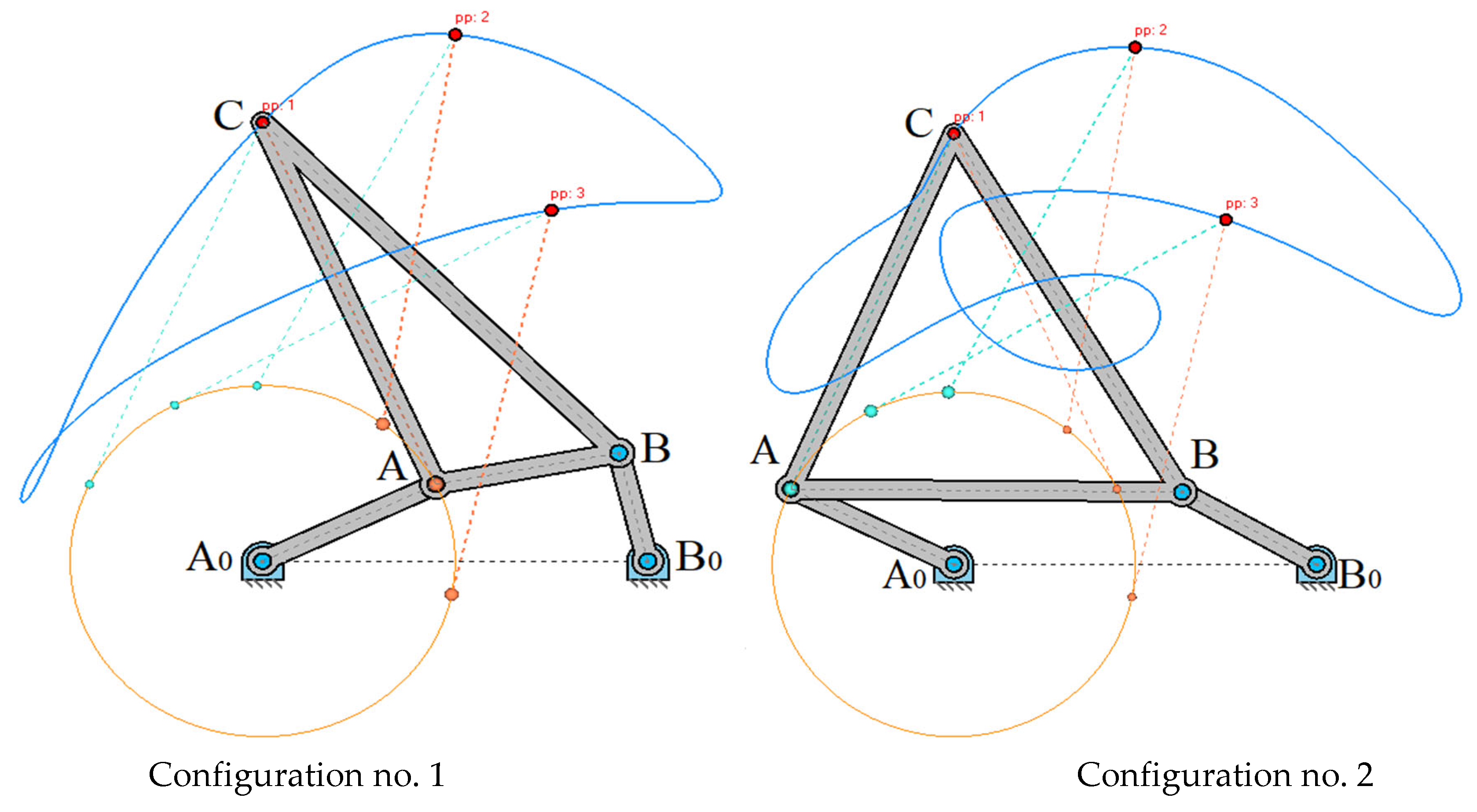
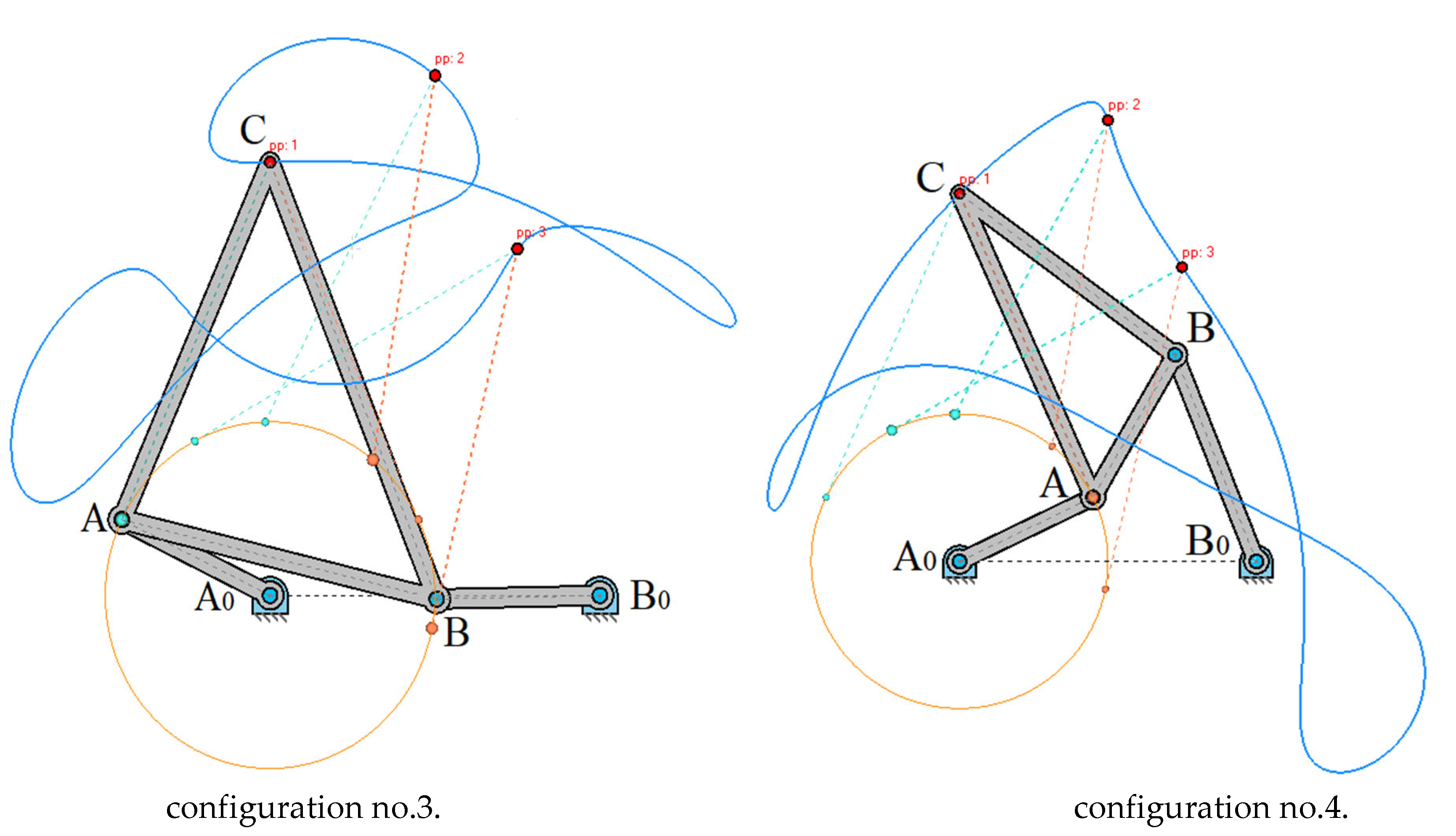
The provided plots illustrate the synthesis mode for a four-bar linkage mechanism, focusing on precision point generation for coupler curve design [36]. The synthesis aims to position the coupler point C, at three specified locations (marked as pp:1, pp:2, and pp:3) along a desired trajectory. The blue curve represents the coupler point’s trajectory, showing how point C moves through the three prescribed precision points. The variations in the trajectory across different plots indicate different configurations and link lengths that satisfy the kinematic synthesis constraints. The mechanism undergoes reconfiguration as it attempts to pass through all three precision points. Some configurations show looping and additional crossings, which suggest alternative kinematic behaviors. The placement of the ground pivots (, ) and the link lengths significantly affect the shape of the coupler curve. In some plots, self-intersecting curves appear, which can indicate higher-order solutions or the presence of unintended dead positions. The ability to match three precision points ensures that the synthesized mechanism [4] can achieve specific motion characteristics with minimal deviation. The similarity between the obtained coupler curves and classical Roberts-type solutions suggests that alternative four-bar mechanisms may generate similar paths. This allows for design flexibility where multiple linkage configurations can be explored.
A more constrained coupler path is generated, ensuring better adherence to the prescribed trajectory, as shown in Figure 12. The additional precision point refines the shape of the coupler curve, making it more predictable and accurate. This configuration improves upon the three-point synthesis by reducing the error between specified positions. The trade-off in complexity and flexibility becomes evident, as more precision points introduce constraints on the linkage design.
The five-point synthesis significantly increases the accuracy of the coupler curve, as shown in Figure 13, ensuring that it passes through all designated precision points with minimal deviation. The computed path exhibits a high level of fidelity to the intended motion. However, the increased number of precision points reduces the flexibility in choosing link dimensions, potentially leading to extreme link ratios or impractical designs. The computational complexity also increases, requiring more sophisticated numerical optimization techniques.
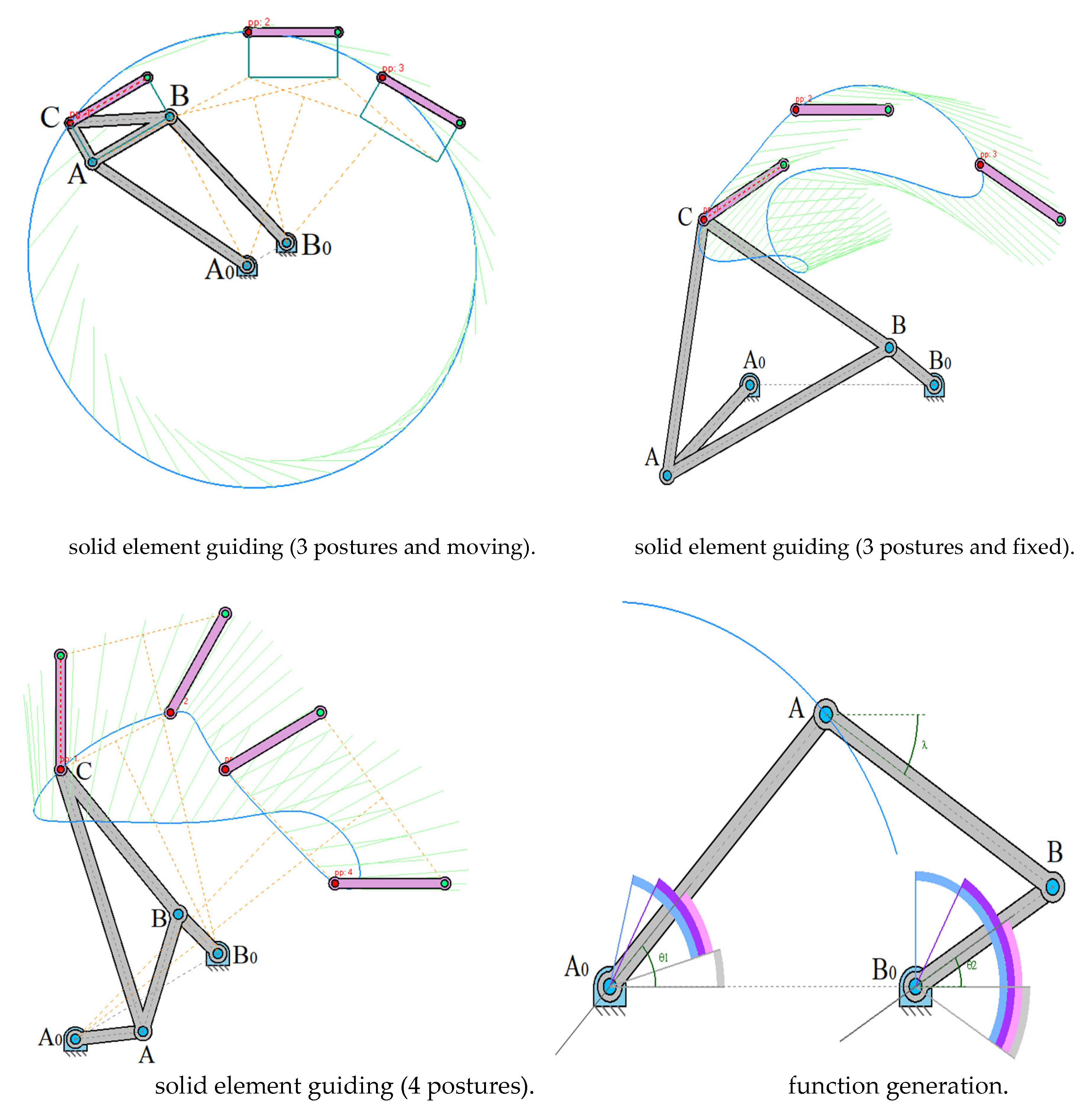
The latest set of computed plots provides further insights into the precision point analysis and function generation of the four-bar linkage:
Shown in Figure 14 (3 postures and moving) three key positions of the coupler. The linkage follows a specific trajectory, hitting the predefined precision points. This setup is suitable for path synthesis [13], where the coupler must pass through three known positions. Illustrates a fixed coupler configuration shown in Figure 14 (3 postures and fixed). Useful for analyzing static configurations where the precision points remain unchanged. Ensures that the linkage remains geometrically constrained during motion. Includes four precision points along the coupler curve shown in Figure 14 (4 postures). This configuration satisfies both position and velocity constraints. Ensures better path control, making it ideal for dwell mechanisms. Displays angular relationships between input and output links shown in Figure 14 (function generation). The angles and define the function generation capability. This analysis is essential for designing linkages that transform motion in a specific manner.
The presented graphs illustrate the kinematic synthesis of mechanisms for different configurations using three, four, and five precision points. These configurations represent attempts to design mechanisms that pass through predefined precision points while maintaining smooth motion characteristics. The synthesized mechanism follows a trajectory passing through three prescribed precision points. The blue curves represent the generated coupler paths, ensuring that the coupler point aligns with the precision points. The selected link dimensions and pivot placements contribute to achieving this motion, with minor deviations due to approximations in the synthesis process [5]. These configurations provide a basic level of control over the motion but may not be sufficient for more complex paths. The addition of a fourth precision point improves the accuracy of the path approximation [30]. The coupler curve exhibits increased fidelity to the desired motion trajectory. Some configurations demonstrate more significant changes in link arrangements to satisfy the additional precision requirement. The increased complexity in synthesis leads to more pronounced deviations in certain positions, highlighting the challenges in maintaining a balance between mechanical feasibility and path accuracy. The five-point synthesis aims to generate a more refined trajectory by enforcing additional geometric constraints. The coupler path aligns more closely with the precision points, indicating better control over the motion. Some configurations show distinct changes in the link lengths and pivot placements, ensuring the mechanism satisfies all five points. This synthesis approach introduces greater sensitivity to minor changes in linkage dimensions, requiring precise design adjustments.
5. Conclusions
This study presents GIM software (Graphical Interface for Mechanisms), an educational and research software designed to simplify kinematic analysis and synthesis of planar mechanisms. The software addresses the challenges students face in understanding kinematics by providing an interactive visualization and computational tool for modeling n-degree-of-freedom (n-DOF) linkages.
a). Educational tool for kinematic analysis:
Supports velocity and acceleration analysis, instant center determination, and coupler curve generation. Enhances student learning by bridging theory and practical application. Integrated into engineering curricula to improve understanding of mechanism design.
b). Advanced computational capabilities:
Allows for real-time modeling, simulation, and motion analysis. Uses complex number representations and matrix-based formulations for accurate calculations. Provides interactive features for exploring mechanism configurations dynamically.
c). Validation and research applications:
Verified against analytical kinematic models and benchmark coupler curves. Used for design optimization, dwell mechanism studies, and function generation. Enables researchers to explore novel mechanism synthesis methods. By integrating geometric modeling, numerical computation, and visualization, GIM enhances both engineering education and kinematic research. It serves as a powerful platform for students and researchers to analyze, synthesize, and optimize mechanical linkages, making it a valuable contribution to mechanism and machine science. The analysis of these computed plots highlights the trade-offs between accuracy, complexity, and feasibility in linkage synthesis. While three precision points provide a basic approximation, four and five-point synthesis improve motion accuracy. Future work should consider integrating numerical optimization techniques and extending the discussion to higher-order synthesis to achieve better results without compromising mechanical feasibility.
Author Contributions
Conceptualization, A.Z.; methodology, A.Z.; software, A.Z.; validation, K.A.; formal analysis, A.A. and Y.K.; investigation, A.Z.; resources, Z.A. and Y.K.; data curation, A.O.; writing—original draft preparation, A.Z., Y.K., and K.A.; writing—review and editing, A.A., Z.A., and A.O.; visualization, A.Z. and A.O.; supervision, A.Z.; project administration, A.Z.; Y.K. and A.A.; funding acquisition, K.A., Z.A., and A.O. All authors have read and agreed to the published version of the manuscript.
Funding
This research was funded by Almaty University of Power Engineering and Telecommunications named after Gumarbek Daukeyev, grant number AP19677356.
Institutional Review Board Statement
The study did not require ethical approval.
Informed Consent Statement
Not applicable.
Data Availability Statement
Data are contained within the article.
Acknowledgments
This work has been supported financially by the research project (AP19677356—To develop systems for controlling the orientation of nanosatellites with flywheels as executive bodies based on linearization methods) of the Ministry of Education and Science of the Republic of Kazakhstan and was performed at Research Institute of Communications and Aerospace Engineering in Almaty University of Power Engineering and Telecommunications named after Gumarbek Daukeyev, which is gratefully acknowledged by the authors.
Conflicts of Interest
The authors declare no conflicts of interest.
References
- Soriano-Heras, E.; Pérez-Carrera, C.; Rubio, H. Mathematical dimensional synthesis of four-bar linkages based on cognate mechanisms. Mathematics 2025, 13, 11. [CrossRef]
- Zhauyt, A.; Alipov, K.; Sakenova, A.; Zhankeldi, A.; Abdirova, R.; Abilkaiyr, Zh. The synthesis of four-bar mechanism. Vibroengineering Procedia 2016, 10, 486-491.
- Kim, J-W.; Seo, T.W.; Kim, J.W. A new design methodology for four-bar linkage mechanisms based on derivations of coupler curve. Mech. Mach. Theory 2016, 100, 138-154. [CrossRef]
- Torres-Moreno, J.L.; Cruz, N.C.; Álvarez, J.D.; Redondo, J.L.; Giménez-Fernandez, A. An open-source tool for path synthesis of four-bar mechanisms. Mech. Mach. Theory 2022,169, 104604. [CrossRef]
- Baskar, A.; Plecnik, M.; Hauenstein, J.D. Finding straight line generators through the approximate synthesis of symmetric four-bar coupler curves. Mech. Mach. Theory 2023, 188, 105310. [CrossRef]
- Liu, W.R.; Si, H.T.; Wang, C.; Jianwei Sun, J.W.; Qin, T. Dimensional synthesis of motion generation in a spherical four-bar mechanism. Trans. Canada. Soci. Mech. Eng. 2024, 48, 1, 94-106. [CrossRef]
- Wang, B.; Du, X.; Ding, J.; Dong, Y.; Wang, C.; Liu, X. The synthesis of planar four-bar linkage for mixed motion and function generation. Sensors 2021, 21, 3504. [CrossRef]
- Wampler, C.W.; Morgan, A.P.; Sommese, A.J. Complete solution of the nine-point path synthesis problem for four-bar linkages. ASME J. Mech. Des. 1992, 114, 153–159.
- Brake, D.A.; Hauenstein, J.D.; Murray, A.P.; Myszka, D.H.; Wampler, C.W. The Complete Solution of Alt–Burmester Synthesis Problems for Four-Bar Linkages. ASME J. Mech. Robot. 2016, 8, 142–149.
- Suh, C.H.; Radcliffe, C.W. Kinematics and Mechanism Design; John Wiley and Sons, Inc.: New York, NY, USA, 1978.
- Ekart, A.; and Markus, A. Using genetic programming and decision trees for generating structural descriptions of four bar mechanisms. AI EDAM 2003, 17, 3, 205 - 220. [CrossRef]
- Kumar, A. Construction of straight-line walking beam eight bar transport mechanism. Inter. J. Sci. Eng. Rese. 2013, 4, 7, 2135-2141.
- Baskar, A., Plecnik, M. Higher order path synthesis of four-bar mechanisms using polynomial continuation. Proc. Adv. Robo. 2021, 15. Springer. [CrossRef]
- Pickard, J.K.; Carretero, J.A.; Merlet, J-P. Towards the appropriate synthesis of the four-bar linkage. Trans. Canada. Soci. Mech. Eng. 2018, 42, 1, 1-9. [CrossRef]
- Bai, S.; and Angeles, J. Coupler-curve synthesis of four-bar linkages via a novel formulation. Mech. Mach. Theory 2015, 94, 177–187.
- Bulatović, R.; and Dordević, S. On the optimum synthesis of a four-bar linkage using differential evolution and method of variable controlled deviations. Mech. Mach. Theory 2009, 44, 1, 235–246.
- Chang, W-T.; Lin, C-C.; Wu, L-I. A note on Grashof's theorem. J. Marin. Sci. Tech. 2005, 13, 4, 239-248.
- Chase, T.; and Mirth, J. Circuits and branches of single-degree-of-freedom planar linkages. J. Mech. Des. 1993, 115, 2, 223–230.
- Lee, W.-T.; Russell, K. Developments in quantitative dimensional synthesis (1970–present): Four-bar path and function generation. Inverse Probl. Sci. Eng. 2018, 26, 1280–1304.
- Sherman, S.N.; Hauenstein, J.D.; Wampler, C.W. Advances in the theory of planar curve cognates. J. Mech. Robot. 2022, 14, 031005.
- Roth, B.; Freudenstein, F. Synthesis of path-generating mechanisms by numerical methods. J. Eng. Ind. 1963, 85, 298–304.
- Hartenberg, R.; Danavit, J. Kinematic Synthesis of Linkages; McGraw-Hill: New York, NY, USA, 1964.
- Soni, A.H.; Harrisberger, L. Roberts’ cognates of space four-bar mechanisms with two general constraints. J. Eng. Ind. 1969, 91, 123–127.
- Jin, S.; Kim, J.; Bae, J.; Seo, T.; Kim, J. Design, modeling and optimization of an underwater manipulator with four-bar mechanism and compliant linkage. J. Mech. Sci. Technol. 2016, 30, 4337–4343.
- Sandor, G.N.; Erdman, A.G. Advanced mechanism design: analysis and synthesis; Prentice-Hall Book Company: Englewood Cliffs, NJ, USA, 1984; Volume 2.
- Jensen, P.W. Synthesis of four-bar linkages with a coupler point passing through 12 points. Mech. Mach. Theory 1984, 19, 149–156.
- Tsai, L.W.; Lu, J.J. Coupler-point-curve synthesis using homotopy methods. ASME J. Mech. Des. 1990, 112, 384–389.
- Subbian, T.; Flugrad, D.R., Jr. Four-bar path generation synthesis by a continuation method. ASME J. Mech. Des. 1991, 113, 63–69.
- Bakthavachalam, N.; Kimbrell, J.T. Optimum synthesis of path-generating four-bar mechanisms. ASME J. Eng. Ind. 1975, 97, 314–321.
- Diab, N.; Smaili, A. Optimum exact/approximated point synthesis of planar mechanisms. Mech. Mach. Theory 2008, 43, 1610–1624.
- Kang, Y.H.; Lee, C.T. The synthesis of four-bar linkages for path generation using hybrid particle swarm optimization. In Proceedings of the First IFToMM Asian Conference on Mechanism and Machine Science, Taipei, Taiwan, 21–25 October 2010; pp. 1–8.
- Zhou, H.; Cheung, E.H.M. Optimal synthesis of crank-rocker linkages for path generation using the orientation structural error of the fixed link. Mech. Mach. Theory 2001, 36, 973–982.
- Shiakolas, P.S.; Koladiya, D.; Keberle, J. On the optimum synthesis of four-bar linkage using differential evolution and the geometric centroid of precision positions. Inv. Probl. Eng. 2002, 10, 485–502.
- Nariman-Zadeh, N.; Felezi, M.; Jamali, A.; Ganji, M. Pareto optimal synthesis of four-bar mechanisms for path generation. Mech. Mach. Theory 2009, 44, 180–191.
- Badduri, J.; Srivatsan, R.A.; Kumar, G.S.; Bandyopadhyay, S. Coupler-curve synthesis of a planar four-bar mechanism using NSGA-II. In Simulated Evolution and Learning; Lecture Notes on Computer Science; Springer: Berlin/Heidelberg, Germany, 2012; Volume 7673, pp. 460–469.
- Romero, N.N.; Campos, A.; Martins, D.; Vieira, R.S. A new approach for the optimal synthesis of four-bar path generator linkages. SN Appl. Sci. 2019, 1, 1504.
Figure 1.
Connecting coupler curve , of the crank-rocker mechanism, consisting of two parts.
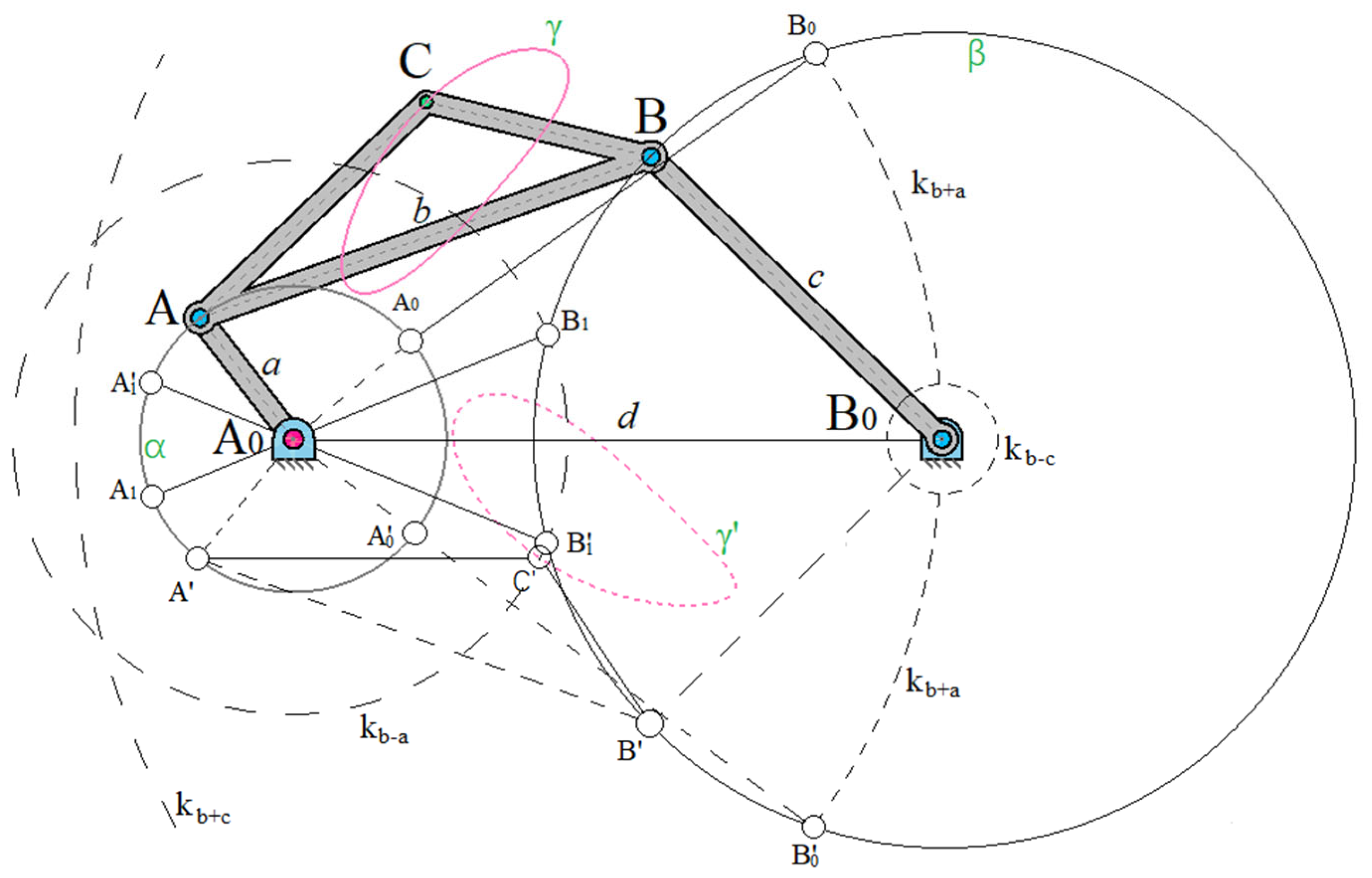
Figure 2.
Connecting coupler curve , of a two-crank mechanism consisting of two parts.
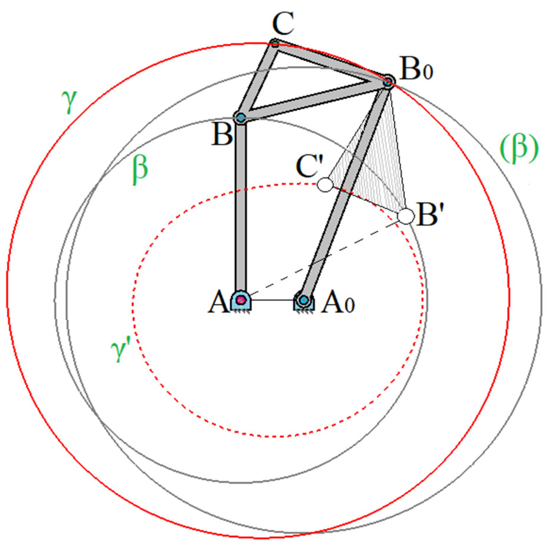
Figure 3.
Dead positions of the double-rocker mechanism.
Figure 4.
Limit crank-rocker mechanism. The connecting coupler curve consists of one part and has double points.
Figure 4.
Limit crank-rocker mechanism. The connecting coupler curve consists of one part and has double points.
Figure 5.
A double-rocker mechanism that does not satisfy the Grashof condition [17]; the connecting coupler curve consists of one part.
Figure 5.
A double-rocker mechanism that does not satisfy the Grashof condition [17]; the connecting coupler curve consists of one part.
Figure 6.
Hinged mechanism for constructing three crank mechanisms according to Roberts' theorem.
Figure 7.
Construction of a connecting coupler curve using three crank mechanisms (solid lines, dotted line, dotted line with dots).
Figure 7.
Construction of a connecting coupler curve using three crank mechanisms (solid lines, dotted line, dotted line with dots).
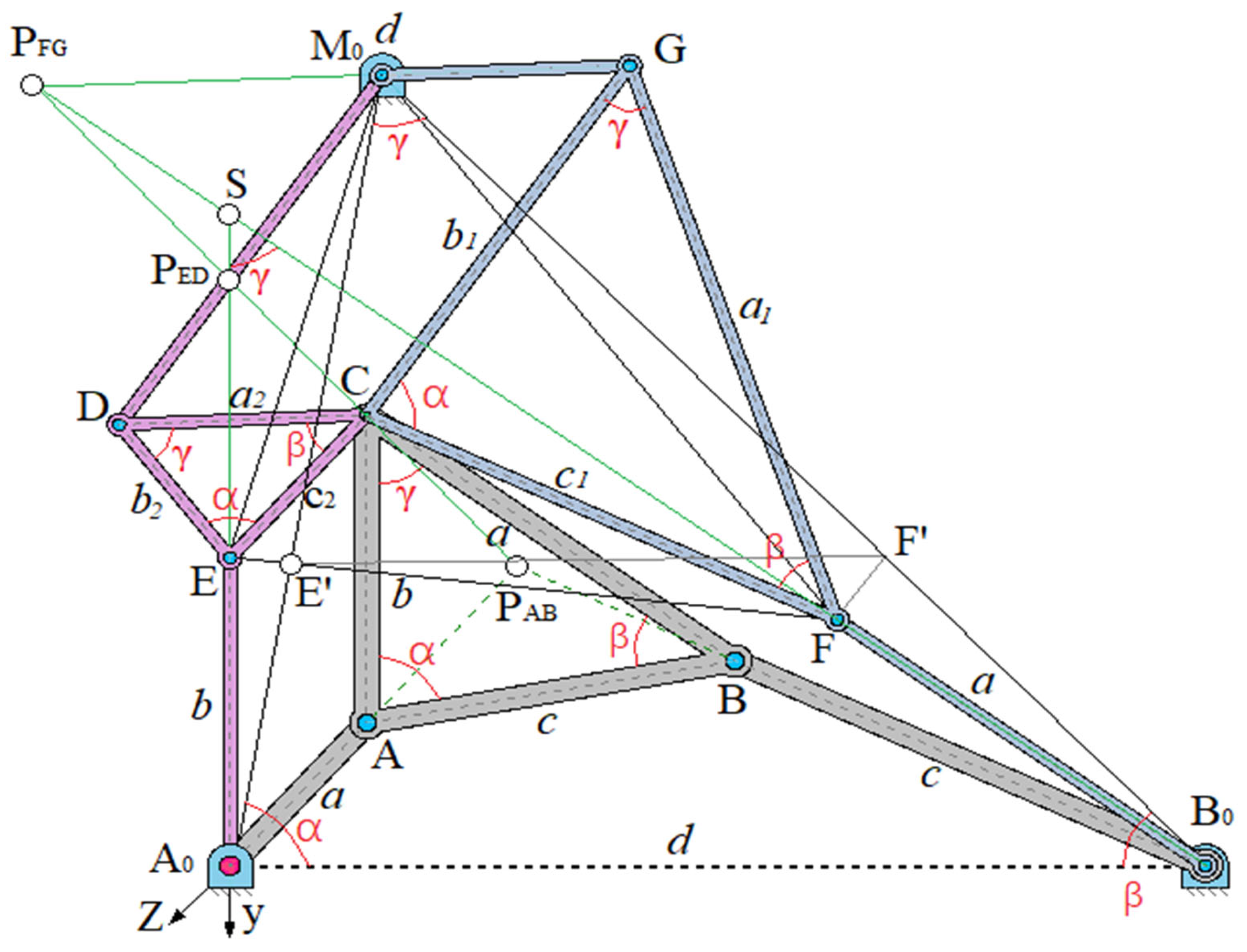
Figure 8.
Three crank mechanisms (top left in one Figure 8, ) are highlighted and arranged side by side.
Figure 8.
Three crank mechanisms (top left in one Figure 8, ) are highlighted and arranged side by side.
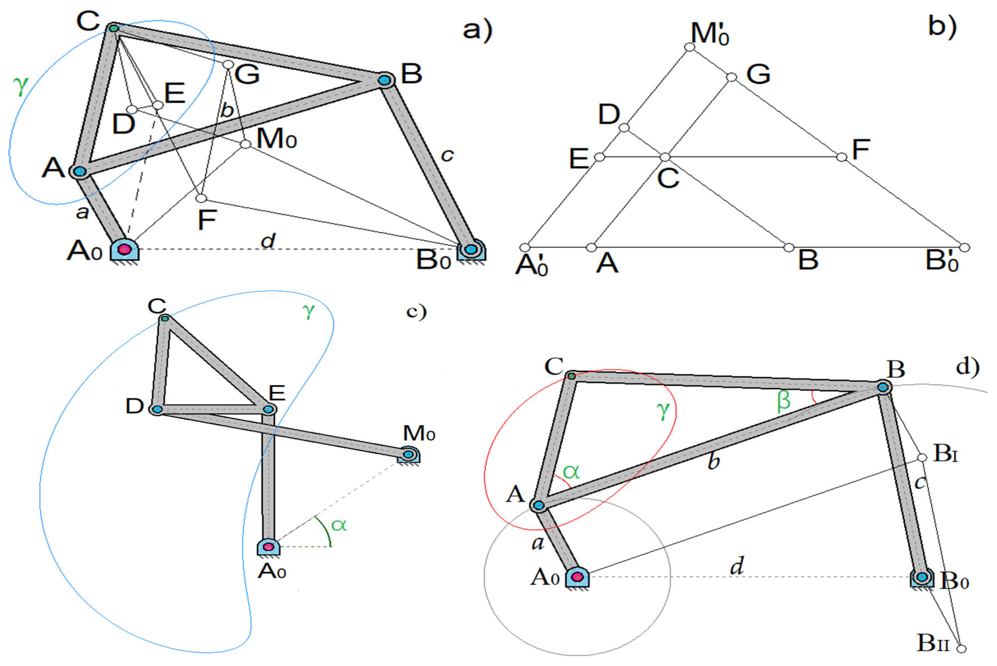
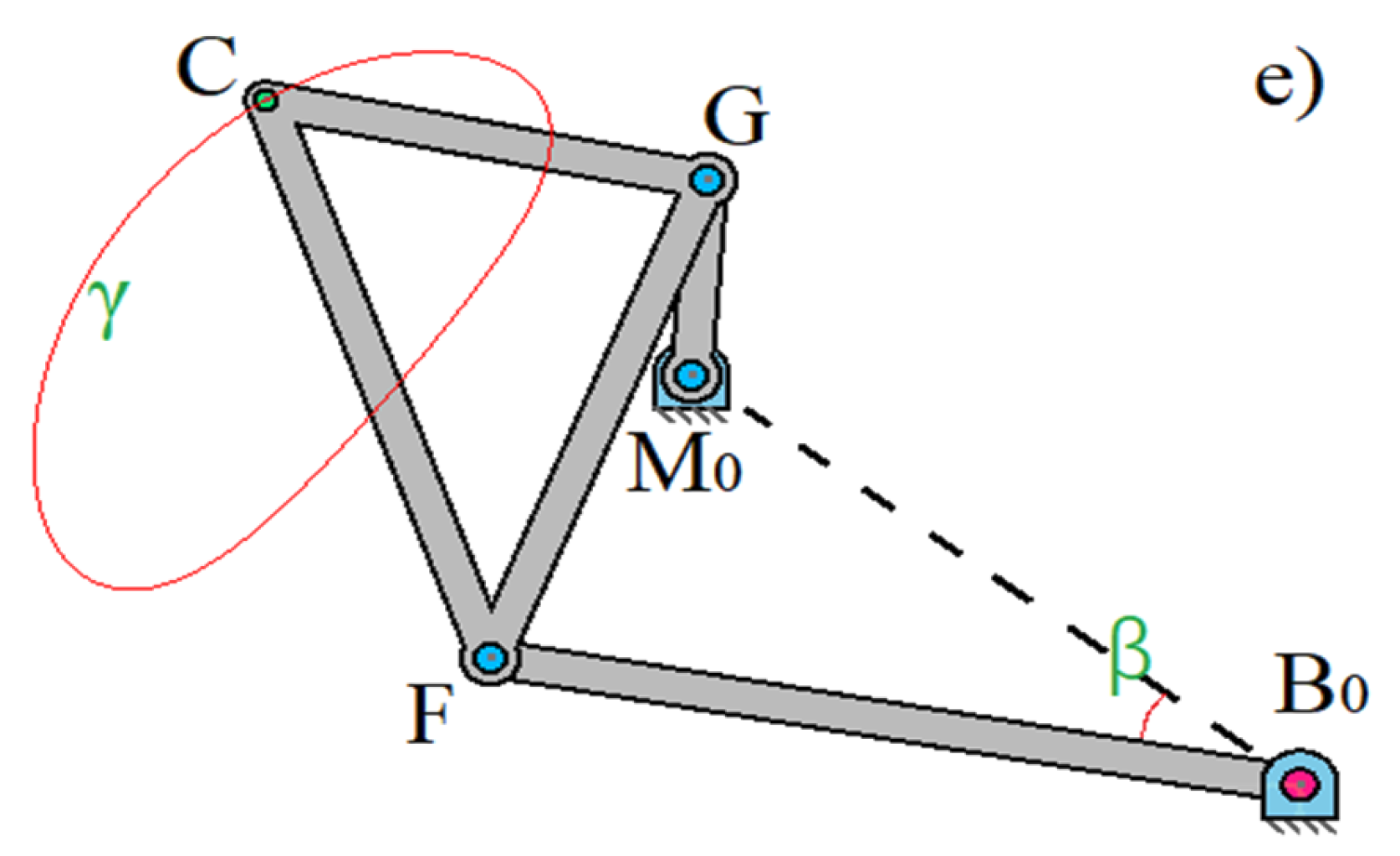
Figure 9.
Parameters for finding the equation of the connecting coupler curve in rectangular coordinates and in complex representation.
Figure 9.
Parameters for finding the equation of the connecting coupler curve in rectangular coordinates and in complex representation.
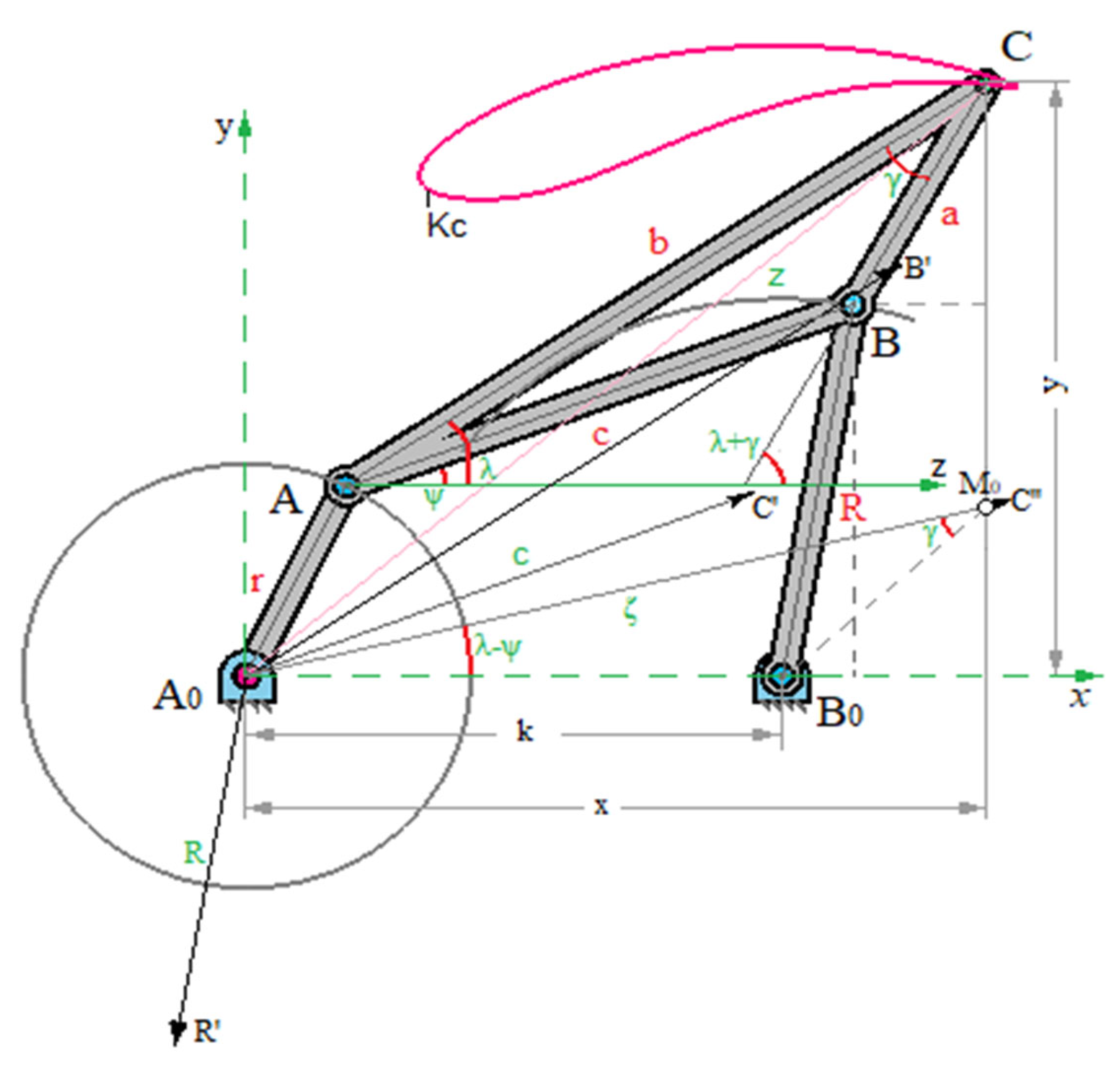
Figure 10.
Double points of the connecting coupler curve on the circle , described around the focal triangle , similar to the connecting rod triangle .
Figure 10.
Double points of the connecting coupler curve on the circle , described around the focal triangle , similar to the connecting rod triangle .
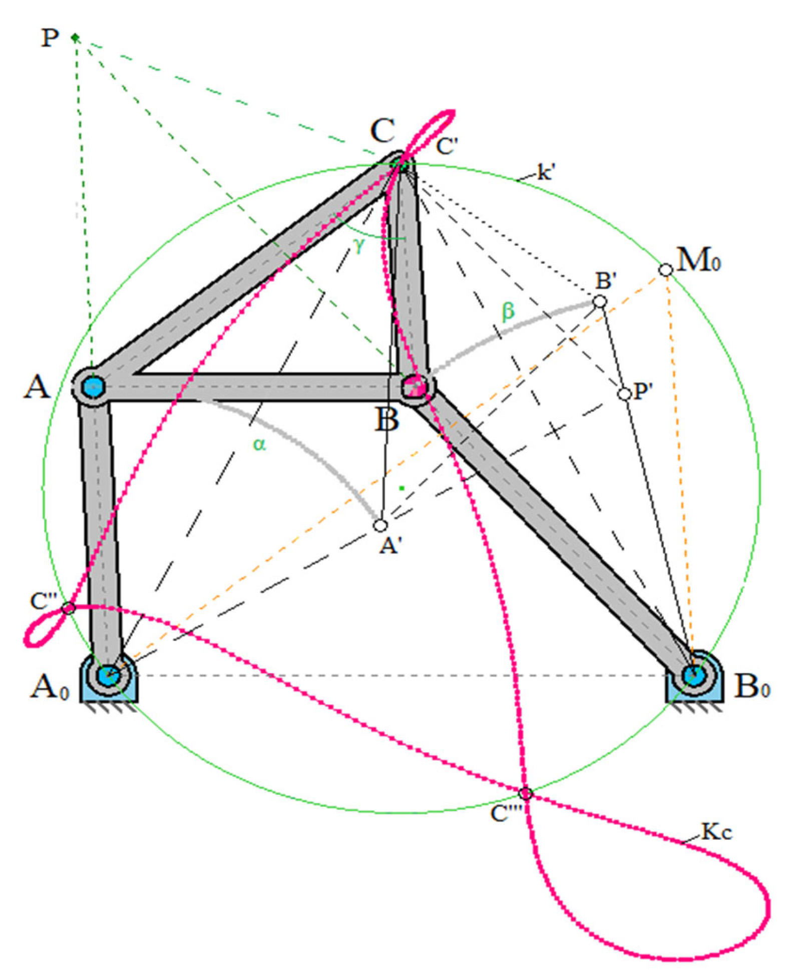
Figure 12.
Computed plot of synthesis mode: precision points (4 points).
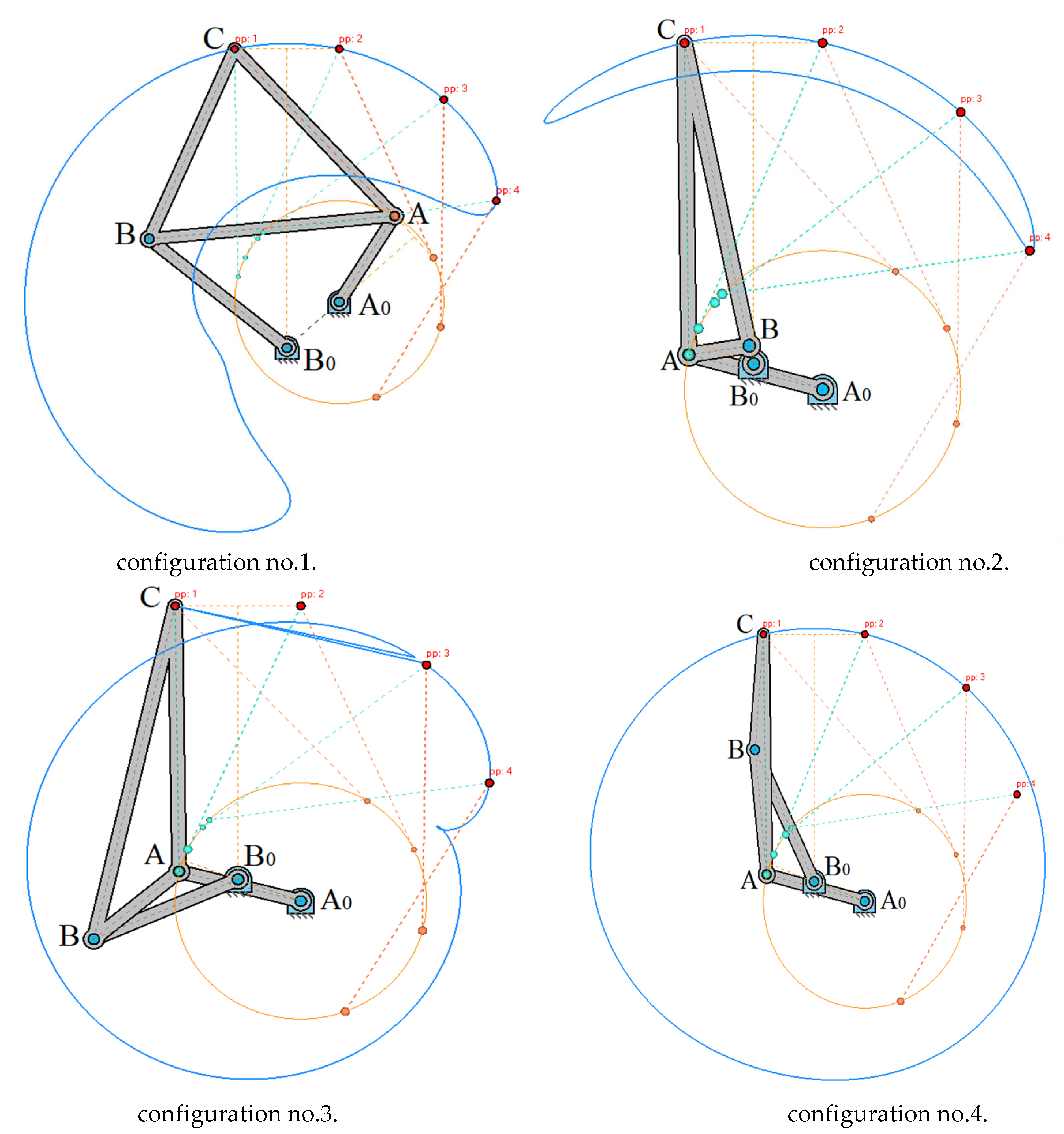
Figure 13.
Computed plot of synthesis mode: precision points (5 points).
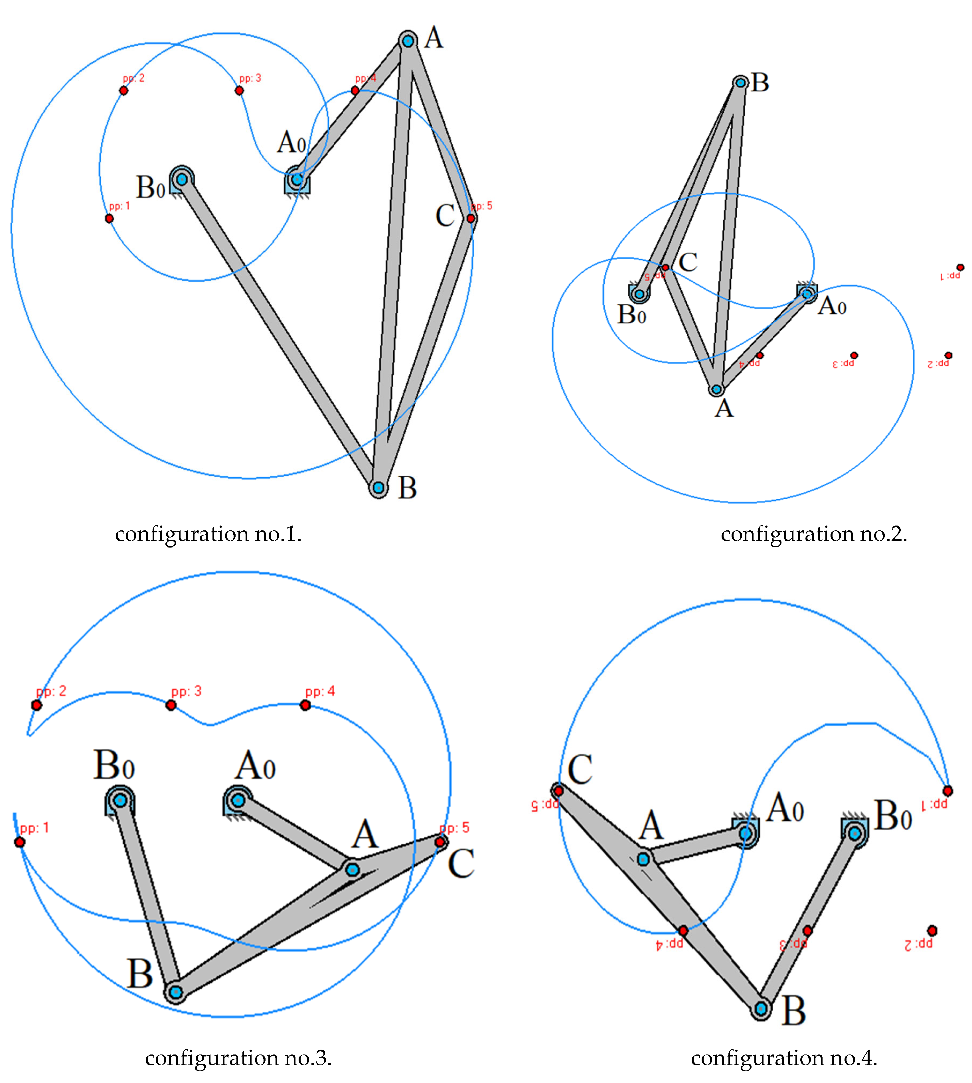
Figure 14.
Computed plot of synthesis mode.
Disclaimer/Publisher’s Note: The statements, opinions and data contained in all publications are solely those of the individual author(s) and contributor(s) and not of MDPI and/or the editor(s). MDPI and/or the editor(s) disclaim responsibility for any injury to people or property resulting from any ideas, methods, instructions or products referred to in the content. |
© 2025 by the authors. Licensee MDPI, Basel, Switzerland. This article is an open access article distributed under the terms and conditions of the Creative Commons Attribution (CC BY) license (http://creativecommons.org/licenses/by/4.0/).
Copyright: This open access article is published under a Creative Commons CC BY 4.0 license, which permit the free download, distribution, and reuse, provided that the author and preprint are cited in any reuse.


