
Submitted:
31 March 2025
Posted:
01 April 2025
You are already at the latest version
Abstract
We explore the post-Newtonian formalism in cosmology, using a system of constituent equations that includes a modified first Friedmann equation—incorporating its homogeneous counterpart—alongside the classical Poisson equation. Furthermore, we include the dynamical equations arising from stress-energy tensor conservation. Within this framework, we examine stellar equilibrium under spherical symmetry. By specifying the equation of state, we derive the corresponding equilibrium configurations. Finally, we investigate gravitational collapse in this context.
Keywords:
First Friedmann equation
; Newtonian mechanics
; conformastat metric
; Stellar equilibrium
1. Introduction
The study of cosmological dynamics has long been rooted in two foundational frameworks: Newtonian mechanics and General Relativity (GR), see the classical books [1,2,3]. While Newtonian theory provides an intuitive and mathematically tractable description of gravitational interactions, particularly in weak-field regimes, GR offers a comprehensive and relativistic description of gravity, essential for understanding phenomena on cosmic scales and in strong-field environments. Bridging these two frameworks has been a central challenge in theoretical cosmology, as it enables a deeper understanding of the interplay between local gravitational interactions and the large-scale structure of the universe.
In this work, we present a metric approach to cosmology based on a previously proposed metric within the class of metric theories of gravity. This framework unifies key aspects of Newtonian mechanics and GR into a coherent formulation. By incorporating the conservation of the stress-energy tensor and a modified non-homogeneous Friedmann equation, our approach seamlessly integrates the classical Poisson equation with the relativistic Hamiltonian constraint. This formulation not only reproduces the standard homogeneous Friedmann equations but also aligns with GR to first order in perturbations, ensuring consistency with observational tests such as the precession of Mercury’s perihelion and the deflection of light (for a detailed discussion, see [4]).
We further explore the implications of this framework in both static and dynamic scenarios. In the static case, our approach yields a conformastatic metric that reduces to the Newtonian potential at large distances while remaining consistent with relativistic predictions. In dynamic settings, we apply the framework to study equilibrium configurations of spherically symmetric stars and the gravitational collapse of pressureless spherical objects. By relating the collapse to the homogeneous Friedmann equations [5,6], we demonstrate the versatility of our approach in describing both local and cosmological phenomena.
Overall, this study establishes a robust and consistent bridge between Newtonian and relativistic descriptions of gravitational interactions, offering an intermediate perspective between Newtonian gravity and GR in the context of cosmological dynamics. By attempting to reconcile these two theoretical frameworks, our approach provides a unified description that captures essential aspects of both classical and relativistic gravity. This formulation not only enhances our understanding of gravitational phenomena across different scales but also offers a framework that remains analytically tractable while preserving key relativistic features.
Furthermore, by integrating elements of Newtonian mechanics with the fundamental principles of GR, our approach sheds light on the transition between weak-field and strong-field regimes, which is crucial for studying astrophysical systems such as galaxies, compact objects, and large-scale cosmic structures. The ability to recover the standard homogeneous Friedmann equations, while also accommodating perturbations consistent with GR, ensures that the model remains compatible with observational constraints, including planetary motion, gravitational lensing, and large-scale structure formation.
The work is structured as follows: In Section 2, we derive the homogeneous Friedmann equations using the principles of Newtonian mechanics. A key element in this derivation is the application of the shell theorem, which allows us to simplify the gravitational interactions in a homogeneous universe and obtain the well-known Friedmann equations. This section highlights the remarkable consistency between Newtonian mechanics and cosmological dynamics in the appropriate regime. In Section 3, we present the post-Newtonian dynamical equations within our proposed framework. These equations extend the Newtonian description by incorporating relativistic corrections, providing a more accurate representation of gravitational interactions in regimes where relativistic effects become significant. This section lays the foundation for bridging the gap between Newtonian and relativistic descriptions of cosmological dynamics. In Section 4, we calculate the metric generated by a point mass particle and demonstrate that our framework, like GR, successfully passes the classical tests of gravity, such as the precession of the perihelion of Mercury and the deflection of light. Section 5 focuses on the application of our approach to a conformastat metric. We explore equilibrium configurations for spherically symmetric systems, showcasing the versatility of our approach in describing static gravitational fields. In Section 6, we investigate gravitational collapse within both Newtonian and post-Newtonian gravity. We analyze the collapse of a pressureless spherical star, establishing a connection between this process and the homogeneous Friedmann equations. Furthermore, we extend this analysis to our post-Newtonian framework, examining how relativistic corrections influence the dynamics of collapse. This section underscores the applicability of our approach to both static and dynamic scenarios, providing a comprehensive understanding of gravitational phenomena across different regimes. We close this work in Section 7 with a brief summary of the entire work.
2. Newtonian Derivation of Friedmann Equations: A Review
As highlighted in several seminal works [7,8], Newtonian mechanics is entirely adequate for describing the dynamics of a homogeneous expanding universe. These studies argue that Newtonian theory correctly predicts the expansion dynamics in regimes where both GR and Newtonian mechanics are equally applicable.
In this section, we review the straightforward and intuitive derivation of the homogeneous Friedmann equations presented in [9] using solely the principles of Newtonian mechanics, in particular, the well-known shell theorem [10]. Therefore, following [9], we consider, in co-moving coordinates, a homogeneous large ball with a radius of in Euclidean space (we can also consider , but for finite radius, the total mass within the ball is finite , where is the mass density). We assume that the ball expands radially. This means that if O is the center of the ball, a point P within the ball at transforms into point at time t, and the distance from O to is given by , where denotes the expansion scale factor of the Friedmann-Lemaître-Robertson-Walker (FLRW) universe given by (here k corresponds to the spatial geometry of the universe).1 Furthermore, at time , we consider the triangle , which transforms into the equivalent triangle at time t. As and , using Thales’ theorem we find that for any points P and Q within the ball, . The relation shows that any ball, at , centered at a point P, expands radially at the same rate as the original large ball. Additionally, the relative velocity between and follows the Hubble-Lemaître law:
The equation of motion for the scale factor in Newtonian mechanics is derived by incorporating the shell theorem [10]. This theorem states that the gravitational field inside a hollow sphere, produced by a homogeneous mass distribution, vanishes. Consequently, in a homogeneous universe, the gravitational force acting on a test particle can be determined by considering only a homogeneous solid sphere centered at the origin 0, where the test particle is located on its boundary. This simplification arises because the gravitational contributions from mass distributions outside this sphere cancel out, allowing the problem to be reduced to the dynamics of the sphere itself.
Then the radial force acting in the test particle is , where is the mass density and is the co-moving vector from the origin to the test particle. Therefore, the acceleration experienced by a probe particle of mass m at the point Q due to the ball is determined by the second Newton’s law as:
which after the elimination of the mass m, leads to the second Friedmann equation for a homogeneous dust field :
This equation can be derived from the Lagrangian:
where represents the mass inside the ball. Indeed, employing the Euler-Lagrange equation yields:
where we have utilized mass conservation:
We observe that the radius R of the chosen ball does not affect the dynamical equations. Thus, we set . To derive the second Friedmann equation for a general fluid field, we must account for the energy associated with the microscopic motion of the particles that constitute the fluid, as well as the interactions between them. Thus, we substitute the mass density with the energy density, namely , in the Newtonian Lagrangian (4) with , resulting in [11]:
Using the Euler-Lagrange equation and the first law of thermodynamics as described in [9,12], one derives the second Friedmann equation . Now, following the techniques as described in Refs. [9,12], one obtains the following
the solution of which is given by [9,12]
where is the constant of integration. Setting to be equal to , one obtains the first Friedmann equation. Finally, considering that the energy of a homogeneous ball of radius a is , the Newtonian Lagrangian appears as , where is the kinetic energy per unit mass and is the gravitational potential generated by the ball with rest mass E.
3. Dynamical Equations in the Post Newtonian Approach
In this section, we present a framework for testing GR under specific assumptions. It is important to emphasize that Einstein’s field equations are fundamentally rooted in the Principle of Equivalence [13,14]. Notably, when this principle was applied to a freely falling observer in a homogeneous gravitational field, it led Einstein to recognize that gravity enters the theory through the metric [15]. However, as highlighted in the literature, the derivation of these equations involved a considerable degree of intuition and heuristic reasoning [4,16,17]. With this in mind, we assess the validity of GR through a modified approach: while retaining the conventional laws governing particle and photon motion within a given metric, we permit deviations in the metric itself from the one predicted by Einstein’s equations—which rely on general covariance and underpin the relativistic theory of gravity.
More specifically, we postulate the conservation of the stress-energy tensor, which is equivalent to the relativistic conservation laws and the Euler equations. Additionally, we consider extensions of the homogeneous first Friedmann equation. These extensions must not only incorporate the classical Poisson equation but also align, at the first order of perturbations, with the well-established Hamiltonian constraint in GR.
The resulting constitutive equations derived within this framework represent an extension of the classical equations of motion. Although these equations are simpler than the full set of Einstein’s field equations—notably lacking general covariance—they retain key insights from GR and satisfy classical tests, as we will demonstrate. This approach enables us to examine the implications of modified metrics while preserving essential physical principles, offering a valuable perspective on the interplay between classical and relativistic descriptions of gravity.
To proceed, we adopt harmonic coordinates [18] and begin with the following line element in the weak-field approximation for a static gravitational field: [1,3],
Here, denotes the physical coordinate. Now, including the expansion of the universe characterized by the scale factor, and the variability of the Newtonian potential, the line element (10), in co-moving coordinates in which , assumes the form below
which is the linear approximation, for a more general metric, namely , of:
where is the perturbed scale factor, which at the first order of perturbations takes the form and plays a crucial role in the understanding of the dynamics of the universe.
The following two important remarks are in order:
- As we will see, our approach falls within the framework of so-called metric theories of gravity [19,20,21]. In this context, we choose a "prior metric" (12), for which the spatial slices are conformally flat, and the conservation of the stress-energy tensor is imposed. Consequently, in addition to the vanishing divergence of the stress-energy tensor, we require an equation to determine . As we will shortly demonstrate, this equation will generalize the first Friedmann equation.
-
To have an intuitive idea about the choice of the metric (12), we apply the the Principle of Equivalence to a uniform gravitational field, namely , and we seek a metric that reproduces Newton’s second law:being the inertial force and the gravitational one, where denotes the acceleration of the body, and we have used the equality of the inertial and gravitational mass.To achieve this, we consider the static line element:and from the minimization of the action , we find:To obtain the Newtonian equation, we must require that the velocity on the right-hand side vanishes. This condition is satisfied when: , being C a constant, which be taken equal to 1 rescaling the co-ordinates. Therefore, we have:and comparing with (13) we find thatwhere b is a constant which must be equal to 1 in order to recover the Minkowski metric when the acceleration vanishes.The conclusion is that, in the case of a homogeneous gravitational field, , the dynamics of a freely falling mass is governed by the Newton’s second law when the acceleration corresponds to the proper acceleration of the free-falling particle. Furthermore, we can assert that the mass does not experience its weight because the proper inertial force precisely compensates for the Newtonian gravitational force.
3.1. First Friedmann Equation
Writing the energy density and the pressure as , , ( indicates the mild variation of the respective quantity) and express the classical Poisson equation as,
which using the co-moving coordinates can be written as:
To reconcile both the equations, we consider the time and the line element becomes . The normal time-like vector is , and with the use of this vector, and taking into account that in the first order of perturbations, , the first Friedman equation, which coincides with the firsts order field equations of GR, can be written as [12]:
where we have introduced the Hubble rate in cosmic time . This equation can be written in a more geometric from considering the gradient of the scale factor :
where we have introduced the Hubble vector with representing the three dimensional gradient. Then, with this notation, in our framework the first Friedmann equation (20) becomes:
where is the square modulus of the Hubble vector and is the Euclidean divergence of the Hubble vector. Note that this equation contains the first homogeneous Friedmann equation and coincides, at the first order of perturbations, with the field equations of GR
Finally, we wish to emphasize that there exist several extensions of the first Friedmann equation, for example: . These extensions incorporate both the homogeneous first Friedmann equation and the classical Poisson equation, and they align, to first order in perturbation theory, with the Hamiltonian constraint in GR. From our perspective, the simplest such extension is:
3.2. Conservation Laws
Introducing the four-velocity where is the space-like velocity, and its dual form, namely , which in a more geometric form can be written in terms of the "flat" operator as where for a given four-vector , one has , we can write the stress tensor as:
The conservation equation is
which leads to the relativistic conservation and Euler equations:
where we have introduced the covariant derivative of a vector , for an scalar , the gradient of a function , and the divergence of a vector . A simple calculation shows that:
- where is the scalar product of the vectors and .
Therefore, the conservation equation becomes:
The Euler equation, which we will obtain from , is:
Summing up, in this approach and disregarding quadratic terms in the velocity , the constituent equations are (here we use as a first Friedmann equation the eq. (24)):
which at first order of perturbations become:
and, are equivalent to the perturbed equations of GR using the Newtonian Gauge (see for example, equations (7.47)-(7.49) of [22]). Effectively, the first equation of (35) coincides with the equation (7.47) of [22]. Next, the third equation of (35) tells us that is a gradient, and thus, performing the temporal derivative of the first equation of (35) and comparing with the second one we find the perturbed version of the so-called diffeomorphism constraint , which is the equation (7.48) of [22] and also , which coincides with the equation (7.49) of [22]. Note also that, inserting the diffeomorphism constraint into the third equation of (35) is another way to find the equation (7.49) of [22].
Finally, we want to stress that the equation (32) coming from the conservation of the stress tensor can be obtained from the first principle of thermodynamics [12]. Effectively, to do it we use the following result:
where is the flow of the fluid, that is, being the identity. Applying this result to the first principle of thermodynamics
where is an infinitesimal volume and the element of volume for our metric is . Applying the previous result, and taking into account that and , we find the equation:
Next, recalling that
because the flow follows geodesics, i.e., , we also have
and thus, obtaining the conservation equation (32).
4. Conformastat Metric: Classical Tests
4.1. Dynamical Equation of Test Particles
We want to find the dynamics of a test particle in the case of a static universe for the conformastat metric (see [23] for details and properties of this metric). The action for a test particle is , with
where we have used the notation and . Performing the calculations we have
and the Euler-Lagrange equation, after introducing the orthogonal rejection of onto , namely , or in terms of the Euclidean inner product , becomes:
which for movements parallels to , i.e., parallels to , leads to the simple dynamical equation . Recalling that in the weak approximation , and the exact result obtained for an homogeneous potential (see eq. (17)), we can define the “exact” Newtonian potential, namely , as , and thus, since we are dealing with an static universe () and potential, the first Friedmann equation (20), which in the static case is the generalization of the classical Poisson equation, and the geodesic equation become:
where is the orthogonal rejection of onto . Using, once again, the Euclidean inner product, we find
which leads to the conservation equation
Finally, for small velocities we disregard the quadratic terms in (43), obtaining:
where we have used that . Taking into account that , and in the week field approximation , we can disregard the quadratic terms on the potential, we find the Newton’s law .
4.2. Metric Produced by a Point Mass Particle
We consider, in a static universe (, the first Friedmann equation (24) looking for the stationary spherical symmetric solution produced by a point particle of mass M situated at the origin of -coordinates. Then we have to solve:
where is the Dirac’s delta function. The well-known solution is this equation, which aligns with the Minkowski metric when is:
where is the Euclidean modulus of . Then, from our definition of the “exact” Newtonian potential:
Finally, to find the relationship with the spherical coordinates, that is between q and the Euclidean distance r, we see that our metric is
with . Since, as was pointed out by Hilbert in [24], the angular term in spherical coordinates is (see also eq. (8.3.4) of [4]), one has:
and, in spherical coordinates, the metric becomes:
which is only singular at ( at ), not like GR, where in spherical coordinates, the metric is singular at the Schwarzschild radius . Note also that, the last approximation of (53) coincides with the post-Newtonian approximation obtained in formula (9.4.25) of [4]. Note that, the geodesic of a radially free falling particle is (43):
which is the Newtonian law for our potential (50). On the other hand, in the approximation , the metric becomes:
which, in this approximation, that is, when , coincides with the Schwarzschild metric:
Two important remarks are in order:
Remark 1.
It is worth noting that the metric (56), commonly referred to as the Schwarzschild metric, was independently derived by Droste [25] and Hilbert [24]. Droste obtained this solution from Einstein’s 1914 “Entwurf” equations [26] without any prior knowledge of Schwarzschild’s work. Hilbert later derived the same result a few months after Droste, approximately one year after Schwarzschild first discovered his family of spherically symmetric solutions to Einstein’s field equations. These solutions describe the gravitational field produced by a point mass located at the origin of the coordinate system.
Among these solutions, Schwarzschild selected the metric that exhibits a singularity solely at the origin. However, through an appropriate coordinate transformation, specifically, using spherical coordinates, this metric reduces to the well-known Schwarzschild form [27].
Remark 2.
The Hilbert-Droste metric can be written in isotropic coordinates as follows [28]:
where . Disregarding quadratic terms on we find:
At this point, it is important to recognize that R is not the radius in spherical coordinates, although it is sometimes identified as such. If one makes this identification, as in [28], it becomes impossible to obtain the correct precession of Mercury’s perihelion. However, by considering the relation between r and R, and disregarding the quadratic terms, one has . Using the correct polar coordinates, we recover the metric (55), which, as we will soon demonstrate, successfully passes the classical test. This observation underscores the fact that it is the physics that guides the accurate interpretation of the coordinates. In other words, the coordinates do not possess an independent meaning separate from the metric solution. Each solution of the metric carries its own physical interpretation of the local coordinates, as exemplified by the Schwarzschild metric (for a more detailed discussion, see [29]).
4.2.1. Precession of the Perihelion
We consider the movement in the plane . Then, in spherical coordinates, the Lagrangian, using the metric (55), will be:
Since the Lagrangian is independent on t and , we have two conserved quantities:
together with the condition , leads to:
That is
and performing the change of variable , we find:
where
Note that taking the derivative with respect , we obtain:
which disregarding the quadratic term on u, is the well-known equation in Newtonian theory, whose solution is the ellipse:
where is the semi latus rectum and e the eccentricity of the ellipse. Next, we introduce the perihelion distance and the aphelion distance. Defining , we see that they are roots of the three-degree polynomial P, because the trajectory reaches its maximum and minimum at . Then, denoting by the other root and following the fundamental theorem of algebra, we have:
where expanding it and comparing with the quadratic term of (64) we find , that is . And we can write:
Therefore, we have the key differential equation:
which coincides with the one obtained using the Schwarzschild solution [30]. To count the angles starting at the perihelion we have to calculate the integral:
To obtain the angle during a revolution we integrate with respect from 0 to , obtaining:
and thus, the precession of the perihelion per revolution is:
where we have used the following relation between the semi latus rectum and .
Remark 3.
In the same way one can calculate the deflection of a beam of light, obtaining the well known result:
where is the distance of closed approach to the origin.
5. Conformastat Metric: Stellar Equilibrium
We will apply our framework to the static case, where the constituent equations become:
where we have used the first Friedmann equation (20), although the same results are obtained using (24). Assuming spherical symmetry, we have:
Integrating the first equation we have
which after another integration and imposing that at infinity, leads to
where is the radius of the star and it mass is . Therefore, the exact Newtonian potential is:
And, for a fixed energy density, the solution of the equation , which can be written as , with initial condition is:
For example, for a constant energy density , one has
and thus, the exact Newtonian potential is:
and the pressure is:
5.1. Linear Equation of State
5.1.1. Exact Solution
We consider the linear EoS (w denotes the barotropic EoS), given the energy density at the boundary, namely , we have
Inserting it into the first equation of (77), we find:
with boundary conditions and , where and .
The mass of the star is:
where
which relates the energy density at the boundary with the mass, that is, given M and , one has:
On the other hand,
which fixes the value of at the boundary. Effectively, defining one has , and thus, the Descartes’ rule of signs combined with Bolzano’s theorem, tells us that this equation only has a positive solution, which fixes . That is, choosing the value of and the mass of the star M, and solving the equation (86) one finds , and thus, solving the equation (90), one obtains and also . Figure 1 presents the numerical solutions of the differential equation (86) considering and taking several values of .
5.1.2. Analytic Solutions
Taking into account that , the first equation of (77) becomes the Lane-Emden equation:
with and .
-
. The Lane-Emden equation becomeswhose solution is , where taking into account the boundary condition , one has:In terms of the q-coordinate:which, of course, coincides with the case of a constant energy density, because implies .
-
. The Lane-Emden equation becomeswhose solution is for , where is the radius of the star in the -coordinate.The mass acquires the form:and the relation at the boundary , leads to:Combining both expressions, we find:whose solution is:provided that, . Therefore, fixing one finds the parameter , and sincewe conclude that, fixing and the mass M, one finds the value of the parameters A, and the radius of the star .
5.1.3. Weak Field Approximation
Considering the EoS, , and taking into account that, in the linear approximation, , the equation , becomes:
and taking the derivative of this equation one gets:
Introducing the dimensionless variables and , the differential equation becomes:
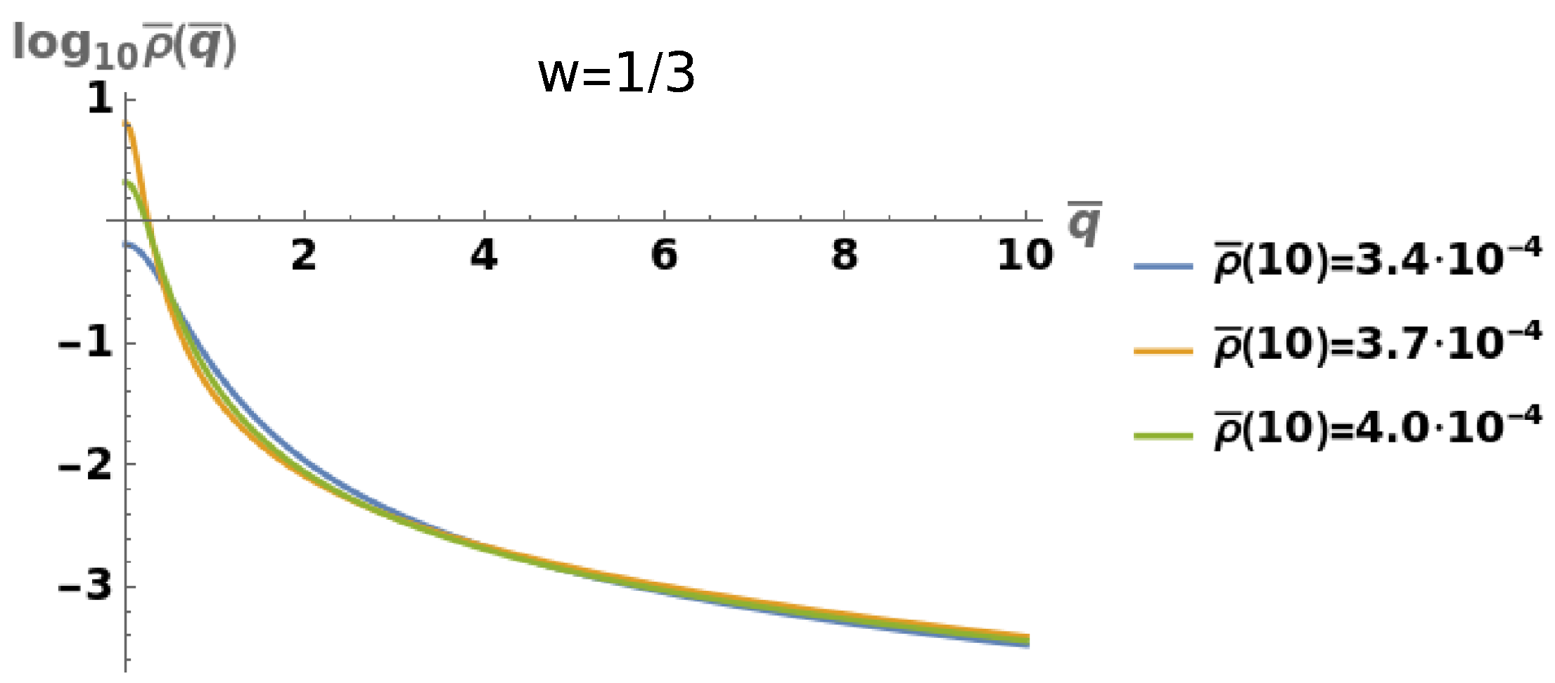
where now the derivative is with respect the dimensionless variable . We have to look for solutions satisfying and fixing the values of and . Then, giving and , we find the energy density and the Newtonian potential in the interior of the star. In Figure 2 we have shown some solutions of the energy density for a fixed value of .
6. Newtonian Gravitational Collapse
In this section we will deal with the gravitational collapse of an homogeneous pressure-less fluid with spherical symmetry in the framework of Newtonian gravity, showing its connection with the homogeneous Friedmann equations.
The Newtonian equations for a pressure-less fluid are:
We look for spherical symmetric solutions. Then, the Newtonian potential has the form:
where is the mass inside the solid sphere of radius q. Due to the spherical symmetry, we write the velocity as , and the conservation equation becomes:
And the Euler’s equation, becomes:
Considering the flux, namely, , with , we can perform the change of coordinates:
where . And, taking into account that , and defining , we have:
We also define , we obtain the equations:
And the Euler equation becomes:
which is the Newton’s law. The boundary condition is , and the initial condition for the energy density is , for a fixed function , satisfying . For the flux , the initial conditions are and , for a given function . Dealing with the mass , we have:
We deal with homogeneous energy densities of the form:
that is:
Then, considering, the evolution as in an expanding or contracting homogeneous universe, the mass acquires the form:
and the Euler equation (113) becomes:
which is the homogeneous second Friedmann equation for a pressure-less fluid. The conservation equation (112) becomes the usual conservation equation in a FLRW universe, that is:
Combining both equations we also obtain the homogeneous first Friedmann equation:
The well-known solution is:
where we have to choose , because , and to have contraction. That is, we have:
We see that the star collapses at the origin at time , and we also have:
and thus, the energy density is:
We also have and
Finally, the Newtonian potential is given by:
and imposing at the boundary , we find:
In terms of the total mass , we have:
6.1. Gravitational Collapse in a Conformastat Metric
We consider a spherical collapse, and we look, in our framework (see [31] for a discussion in the context of GR) for the geodesical evolution of the radius, which in this subsection we will denote by Q in q-coordinate, of the star. The exterior metric is given by
where . Since the boundary moves radially, the Lagrangian is given by:
Since the exterior metric is static we have the conservation law:
where E is a dimensionless constant. To simplify the calculations we take , obtaining . Using the constraint , we find:
and the solution, as a function of the proper time, is given by:
And thus, we can solve , obtaining:
where
Note that the metric becomes singular when
This stands in stark contrast to the Newtonian case, where, from the perspective of an external observer, the singularity is reached within a finite time. Finally, it is important to note that when , analogous results can be derived, albeit with more complex analytical expressions. The underlying methodology remains consistent, but the increased complexity in the mathematical formulations necessitates a more intricate analysis. Effectively, when , the equation (134) becomes:
where we have performed the change of variable . Tanking into account that,
one finds an implicit expression of the form:
where it is impossible to analytically isolate as a function of the proper time.
7. Conclusions
In the present work, we have presented some metric theories of gravitation leading to a post-Newtonian approach to cosmology. This approach is based on a system of equations comprising the conservation of the stress-energy tensor and a non-homogeneous first Friedmann equation. This modified Friedmann equation incorporates both the standard homogeneous Friedmann equation and the classical Poisson equation. Furthermore, it aligns, to first order in perturbations, with the Hamiltonian constraint derived from the field equations in GR.
In the static case, our framework yields a conformastat metric. For a point mass particle located at the origin of the coordinate system, this metric exhibits a singularity solely at the origin and reduces to the Newtonian potential at large distances from the origin. Moreover, this metric reproduces the same predictions for the precession of the perihelion of Mercury and the deflection of light as those derived from GR. Thus, the framework maintains consistency with both Newtonian gravity in the weak-field limit and key observational tests of GR.
We have also applied our framework to investigate equilibrium configurations of spherically symmetric stars. Additionally, we have examined the gravitational collapse of a pressure-less spherical star within the context of Newtonian theory, establishing a connection between this collapse and the homogeneous Friedmann equations. Furthermore, we have analyzed the collapse within our proposed approach, extending the analysis beyond the Newtonian framework to explore its implications in a more general setting.
In essence, we have demonstrated that our framework establishes a consistent and rigorous bridge between Newtonian and relativistic descriptions of cosmological dynamics. By unifying the key elements of Newtonian mechanics, such as, the Poisson equation, with the relativistic framework of GR, our approach captures the essential features of both theories. This is evident by its ability to reproduce the homogeneous Friedmann equations, aligned with the Hamiltonian constraint of GR to first order in perturbations, and correctly predict phenomena such as the precession of the perihelion of Mercury and the deflection of light. Furthermore, the framework’s applicability to both static and dynamic scenarios, including the analysis of equilibrium stellar configurations and gravitational collapse, underscores its versatility and robustness. Thus, our work provides a comprehensive and coherent methodology for transitioning between Newtonian and relativistic regimes, offering valuable insights into the interplay between these two foundational descriptions of gravitational physics.
Acknowledgments
We would like to thank Llibert Aresté-Saló for helping in performing the numerical calculations. JdH is supported by the Spanish grant PID2021-123903NB-I00 funded by MCIN/AEI/10.13039/501100011033 and by “ERDF A way of making Europe”. SP has been supported by the Department of Science and Technology (DST), Govt. of India under the Scheme “Fund for Improvement of S&T Infrastructure (FIST)” (File No. SR/FST/MS-I/2019/41).
References
- Einstein, A. The Meaning of Relativity; Princeton University Press: Princeton, 1953. [Google Scholar]
- Pauli, W. Theory of Relativity; Dover Books on Physics, Pergamon Press, 1981.
- Landau, L.D.; Lifschits, E.M. The Classical Theory of Fields; Vol. Volume 2, Course of Theoretical Physics, Pergamon Press: Oxford, 1975. [Google Scholar]
- Weinberg, S. Gravitation and Cosmology: Principles and Applications of the General Theory of Relativity; John Wiley and Sons: New York, 1972. [Google Scholar]
- Friedman, A. On the Curvature of space. Z. Phys. 1922, 10, 377–386. [Google Scholar] [CrossRef]
- Friedmann, A. On the Possibility of a world with constant negative curvature of space. Z. Phys. 1924, 21, 326–332. [Google Scholar] [CrossRef]
- McCREA, W.H.; MILNE, E.A. NEWTONIAN UNIVERSES AND THE CURVATURE OF SPACE. The Quarterly Journal of Mathematics, /: 73–80, [https, 4481; -5. [Google Scholar] [CrossRef]
- Callan, C.; Dicke, R.H.; Peebles, P.J.E. Cosmology and Newtonian Mechanics. American Journal of Physics 1965, 33, 105–108. [Google Scholar] [CrossRef]
- de Haro, J. Relations between Newtonian and Relativistic Cosmology. Universe 2024, arXiv:gr-qc/2406.11936]10, 263. [Google Scholar] [CrossRef]
- Newton, I. Philosophiae Naturalis Principia Mathematica.; 1687. [CrossRef]
- Minazzoli, O.; Harko, T. New derivation of the Lagrangian of a perfect fluid with a barotropic equation of state. Phys. Rev. D 2012, arXiv:gr-qc/1209.2754]86, 087502. [Google Scholar] [CrossRef]
- de Haro, J.; Elizalde, E.; Pan, S. On the Perturbed Friedmann Equations in Newtonian Gauge. Universe 2025, arXiv:gr-qc/2412.15139]11, 64. [Google Scholar] [CrossRef]
- Einstein, Albert. How I created the theory of relativity, lecture given in Kyoto on 1922. 14 December.
- Norton, J. What was Einstein’s principle of equivalence? Stud. Hist. Philos. Sci. A 1985, 16, 203–246. [Google Scholar] [CrossRef]
- Schwartz, H.M. Einstein’s comprehensive 1907 essay on relativity, part III. American Journal of Physics 1977, 45, 899–902. [Google Scholar] [CrossRef]
- Wilczek, F. Total Relativity: Mach 2004, 2004. [CrossRef]
- Elizalde, E. Einstein, Barcelona, Symmetry & Cosmology: The Birth of an Equation for the Universe. Symmetry 2023, 15, 1470. [Google Scholar] [CrossRef]
- Fock, V. The Theory of Space, Time and Gravitation; Pergamon, 2015.
- Thorne, K.S.; Will, C.M. Theoretical Frameworks for Testing Relativistic Gravity. I. Foundations. Astrophys. J 1971, 163, 595. [Google Scholar] [CrossRef]
- Will, C.M. Theoretical Frameworks for Testing Relativistic Gravity. II. Parametrized Post-Newtonian Hydrodynamics, and the Nordtvedt Effect. Astrophys. J. 1971, 163, 611. [Google Scholar] [CrossRef]
- Ni, W.T. Theoretical Frameworks for Testing Relativistic Gravity.IV. a Compendium of Metric Theories of Gravity and Their POST Newtonian Limits. Astrophys. J. 1972, 176, 769. [Google Scholar] [CrossRef]
- Mukhanov, V. Physical Foundations of Cosmology; Cambridge University Press: Oxford, 2005. [Google Scholar] [CrossRef]
- Synge, J. Relativity: The General Theory; Number v. 1 in North-Holland series in physics, North-Holland Publishing Company, 1960.
- Hilbert, D. The Foundations of Physics. Nachr. Ges. Wiss. Göttingen, 1917, pp. 53–76.
- Droste, J. The field of a single centre in Einstein’s theory of gravitation, and the motion of a particle in that field. Proc. K. Ned. Akad. Wet., Ser. A 1917, 19, 197–215. [Google Scholar] [CrossRef]
- Einstein, A.; Grassmann, M. Outline of a Generalised Theory of Relativity and of a Theory of Gravitation. Zeitschrift Fur Mathematik and Physik 1913, 62, 225–261. [Google Scholar]
- Schwarzschild, K. On the gravitational field of a mass point according to Einstein’s theory. Sitzungsber. Preuss. Akad. Wiss. Berlin (Math. Phys.) 1916, 1916, 189–196. [Google Scholar]
- Eddington, A.S. The Mathematical Theory of Relativity; The University Press: Cambridge [Eng.], 1930. [Google Scholar]
- Johns, O.D. Validity of the Einstein hole argument. Studies in the History and Philosophy of Modern Physics 2019, arXiv:physics.hist-ph/1907.01614]68, 62–70. [Google Scholar] [CrossRef]
- Magnan, C. Complete calculations of the perihelion precession of Mercury and the deflection of light by the Sun in general relativity 2007. arXiv:gr-qc/0712.3709].
- Balakrishna, J.; Bondarescu, R.; Moran, C.C. Self-gravitating stellar collapse: explicit geodesics and path integration. Front. Astron. Space Sci. 2016, arXiv:gr-qc/1501.04250]3, 29. [Google Scholar] [CrossRef]
| 1 | Without any loss of generality we assume that the present day value of the scale factor is unity, i.e., with . |
Figure 1.
Different solutions of Equation (86) for several values of the parameter .
Figure 1.
Different solutions of Equation (86) for several values of the parameter .
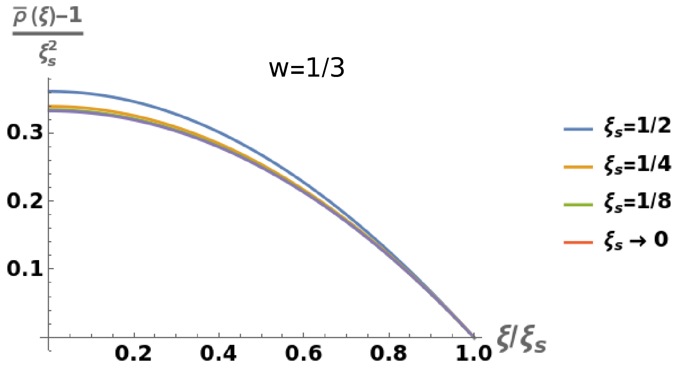
Figure 2.
Different values of the energy density in logarithmic scale for fixed values of the energy density at .
Figure 2.
Different values of the energy density in logarithmic scale for fixed values of the energy density at .
Disclaimer/Publisher’s Note: The statements, opinions and data contained in all publications are solely those of the individual author(s) and contributor(s) and not of MDPI and/or the editor(s). MDPI and/or the editor(s) disclaim responsibility for any injury to people or property resulting from any ideas, methods, instructions or products referred to in the content. |
© 2025 by the authors. Licensee MDPI, Basel, Switzerland. This article is an open access article distributed under the terms and conditions of the Creative Commons Attribution (CC BY) license (http://creativecommons.org/licenses/by/4.0/).
Copyright: This open access article is published under a Creative Commons CC BY 4.0 license, which permit the free download, distribution, and reuse, provided that the author and preprint are cited in any reuse.


