
Submitted:
19 January 2026
Posted:
20 January 2026
You are already at the latest version
Abstract
The multimessenger constraint on the speed of gravitational waves, |c_T/c - 1| ≤ 10^-15, provides a powerful discriminator among modified-gravity scenarios. In this work, we perform a fully phenomenological and data-driven test of a symmetry-motivated weak-field limit that yields MOND-like dynamics governed by a single, global, dimensionless parameter ε (epsilon). This framework predicts three linked consequences: (1) the MOND acceleration scale emerges as a_0 = εcH_0; (2) the observed diversity of galaxy rotation curves is controlled by a geometry-only efficiency factor κ ≈ <h/r>; and (3) the galactic parameter a_0 and the cosmological parameter Ω_Λ share a common origin through ε.We test these predictions using a full-likelihood analysis of the SPARC rotation-curve sample. The model is decisively preferred over standard MOND, with ΔBIC ≈ 38. A novel galaxy-thickness test confirms the geometric nature of κ, revealing a strong correlation (R^2 ≈ 0.818) between the dynamically inferred efficiency, disk thickness, and surface density. Finally, a cross-scale consistency check shows that κ naturally reconciles the galactic and cosmological determinations of ε.These results demonstrate that this single-parameter weak-field limit provides a predictive and observationally consistent description of several long-standing empirical regularities, while remaining compatible with the gravitational-wave speed constraint.
Keywords:
modified gravity
; gravitational-wave speed
; MOND phenomenology
; galaxy rotation curves
; PT symmetry
; information criteria
1. Introduction
The joint observation of GW170817 and GRB170817A established that gravitational waves travel at the speed of light with exquisite precision, [2]. This single measurement acts as a formidable guillotine for a vast landscape of modified gravity theories. Concurrently, persistent mass discrepancies in galaxies and clusters continue to motivate alternatives to cold dark matter, most notably Modified Newtonian Dynamics (MOND) [7]. This creates a dual challenge for any viable theory of gravity: it must (i) respect the strict luminality constraint without fine-tuning, and (ii) simultaneously account for the empirical regularities of disk galaxy kinematics.
A PT-symmetric quaternionic (PTQ) geometry was recently proposed to meet the first challenge from first principles [1]. Its theoretical structure combines a PT-scalar observable map with projective equivalence in a metric-affine (Palatini) setting. In the tensor sector, these symmetries enforce a coefficient-locking identity at quadratic order (), thereby fixing structurally, rather than by tuning parameters [1].
- Classification disclaimer (to prevent a common misreading).
In the weak-field regime relevant to galaxies, the PTQ scalar observable channel admits IR expressions that can look “scalar-like.” However, this manuscript does not introduce a propagating matter scalar, nor does it use a scalar Stueckelberg field to realize full projective invariance. Instead, we adopt the Route-A posture: projective equivalence is implemented by a one-form compensator (treated as a non-dynamical spurion), and the scalar channel is built from the already invariant residue . A scalar potential appears only as a background longitudinal representative on admissible domains where implies ; crucially, is not a compensator. These conventions and their observable meaning are fixed in Section 2 (and Appendix A).
This work addresses the second challenge by developing and testing the PTQ framework’s predictions for disk galaxies. In its late-time, weak-field limit, the theory yields a one-parameter cosmology–galaxy dictionary governed by a single, global, dimensionless parameter . This leads to a predictive structure for galactic dynamics, encapsulated in three core hypotheses that form the roadmap of this paper:
- (1)
- Global Viability: The PTQ weak-field limit provides a statistically superior description of galaxy rotation curves compared to standard MOND. This relies on the prediction that the MOND acceleration scale is directly tied to the Hubble constant, .
- (2)
- Geometric Origin of Diversity: The observed diversity in rotation curves is governed by a predictable, geometry-only efficiency factor , which quantifies how a finite-thickness disk intercepts the background field.
- (3)
- Cross-Scale Consistency: The single parameter provides a consistent link between the cosmological dark energy density, , and galactic dynamics. The framework’s internal consistency can be tested by checking whether the values of inferred from cosmology and from galaxies can be reconciled through the geometric factor .
By systematically testing these interconnected hypotheses against observational data, we will demonstrate that the PTQ framework offers a unified and empirically successful route to the dark-universe phenomenology while remaining compatible with the gravitational-wave speed constraint.
- Organization.
Section 2 summarizes the Route-A + PT-projector posture and the resulting low-energy dictionary. Section 3 defines the likelihood analysis on SPARC and the model families used in the fits. Section 5 presents the population inference for , the thickness-based audit of , and the cross-scale consistency check. Appendices provide derivations of the project-first scalar map, the cosmology normalization, and reproducibility details.
2. The PTQ Framework: Principles and Low-Energy Predictions
The empirical tests in the subsequent sections rely on a disciplined symmetry posture developed in Ref. [1]. This section summarizes the parts of that posture needed for the present weak-field program and makes explicit the “observable map” that prevents common misclassifications (e.g., as a generic scalar–tensor theory).
Symbol map (roles in this manuscript).
- Compensator (Route A): a one-form implementing full projective equivalence; in the phenomenological spurion posture it is non-dynamical (not a propagating degree of freedom).
- Invariant residue: the projectively invariant one-form , where is the torsion trace.
- Scalar representative: a potential used only in the scalar observable channel on admissible domains where so that . Importantly, is not a compensator.
Throughout, we adopt a project-first convention: scalar observables are defined by applying the PT-scalar projector (denoted ) before evaluation (see Appendix A).
2.1. Core Principles: PT Symmetry and Projective Invariance
The PTQ framework is formulated in a metric-affine (Palatini) geometry where the metric and connection are treated as independent variables. The observable sector is then carved out by (i) a PT-scalar projection selecting the real PT-even scalar algebra, and (ii) projective equivalence implemented in its full one-form orbit (Route A).
2.1.1. Palatini Variables and Full Projective Equivalence (the One-Form Orbit)
A metric-affine connection admits the projective shift
The torsion tensor is defined by the antisymmetric part of the connection,
and is a bona fide tensor (in contrast to , which is gauge-like and not a tensor).
A key point for later interpretation is that a scalar Stueckelberg completion can only compensate an exact subset of the projective orbit, , and therefore does not realize the full one-form equivalence class. The posture adopted in this paper is therefore based on the full orbit from the outset (Route A).
2.1.2. Route A: One-Form Compensator and the Invariant Residue
To implement full projective equivalence in the observable sector, we introduce a one-form compensator that transforms as
so that the combination
is invariant by construction under the full projective shift. This is the only torsion-trace object allowed to enter the scalar observable dictionary used in the weak-field analysis.
- Spurion posture (no extra propagating sector).
In the phenomenological regime studied here, is treated as a spurion: it is a non-dynamical bookkeeper that enforces the symmetry in the observable map, and it does not introduce an additional propagating degree of freedom. Operationally, the scalar-channel variation and all low-energy constructions are expressed in terms of the already invariant residue rather than in terms of a new dynamical compensator field.
2.1.3. Scalar PT Projector and the Observable Map
The PTQ framework distinguishes underlying geometric structure from the observable scalar algebra. The latter is selected by the PT-scalar projector , which maps quaternionic-valued scalars to their real, PT-even sector. Concretely, we define the scalar observable sector by
This is an observable selection rule: it fixes which scalar densities are admissible in the action and in the IR dictionary. It should not be conflated with a statement that other (e.g., quaternionic or u-odd) structures are absent in the underlying geometry; rather, they do not contribute to by construction under the project-first rule.
- Projection vs. truncation.
The PT projector removes PT-odd/pseudoscalar contributions from the scalar algebra. Separately, the phenomenological truncation adopted in this manuscript restricts attention to a scalar-channel dictionary built from (and the PT-even metric sector). In particular, the exclusion of additional torsion components (e.g., axial or traceless irreducible parts) is a truncation choice consistent with the posture, not something the PT projector is claimed to accomplish by itself. This distinction prevents a common misreading in which parity-even objects outside the chosen scalar algebra are incorrectly attributed to a failure of .
2.1.4. Scalar-Channel Focus and the Longitudinal Representative
The empirical program of this paper is deliberately restricted to the scalar observable channel relevant to late-time, weak-field galactic dynamics. In this channel we impose, on admissible domains, the integrability condition
so that admits a longitudinal representative,
Hard classification anchor.ϵ isnota compensator; it is only a background longitudinal representative of the already invariant one-form used in the scalar observable channel. This is the precise sense in which scalar-like IR expressions arise in the weak-field dictionary without introducing a generic propagating scalar–tensor sector.
- Luminal tensor sector (structural, not tuned).
As proven in Ref. [1], the combined posture (project-first PT-even scalar algebra plus projective completion) enforces a coefficient-locking identity in the quadratic tensor action (), and therefore fixes without parameter fine-tuning, consistent with GW170817.
2.2. Weak-Field, Late-Time Posture: MOND Phenomenology and the Dictionary
In the late-time weak-field regime relevant to disk galaxies, the scalar-channel dictionary collapses to a one-parameter description governed by a single global dimensionless parameter (a constant in this phenomenological analysis). The resulting cosmology–galaxy map can be summarized as
Here is a derived geometric efficiency, not an additional free parameter. It quantifies how a finite-thickness disk intercepts the isotropic background acceleration scale set by . The PTQ weak-field posture predicts (see Appendix B.4), providing a concrete geometric mechanism for rotation-curve diversity and BTFR scatter.
The empirical program is thus: (i) infer a single population-level and test global viability against the SPARC likelihood, and (ii) audit the geometric nature of the inferred efficiency against thickness proxies. We formalize these tests in Section 3; reproducibility commands are provided in Appendix D.
2.3. Minimal Cosmology Map: From Action to
To emphasize that the cosmology–galaxy dictionary is predictive rather than postulated, we summarize an auditable derivation of the first two entries of Eq. (8). Full details and normalizations are provided in Appendix A and Appendix A.4.
- The Project-First Action.
As per the project-first rule, all scalar observables are defined using the PT-scalar projector applied before evaluation. We begin with the quaternionic split of the metric
and the dimensionless imaginary blocks that encode the IR deformations,
The Einstein–Hilbert action is then constructed in the project-first form:
- Derivation of the Effective Density.
Using the exact projected measure from Appendix A.3, we expand both and to second order in the small parameters and . All PT-odd (u-odd) contributions to scalar densities are removed by the PT projection, yielding a real PT-even scalar density,
where is a geometry-independent coefficient derived from the and terms (see Appendix A for closed forms). Identifying the constant term in Eq. (12) as an effective vacuum energy density,
we define the dark-energy density parameter as
To align with standard FRW conventions, we set the normalization constant (see Appendix A.4 for details). This yields the cosmology map used throughout the paper:
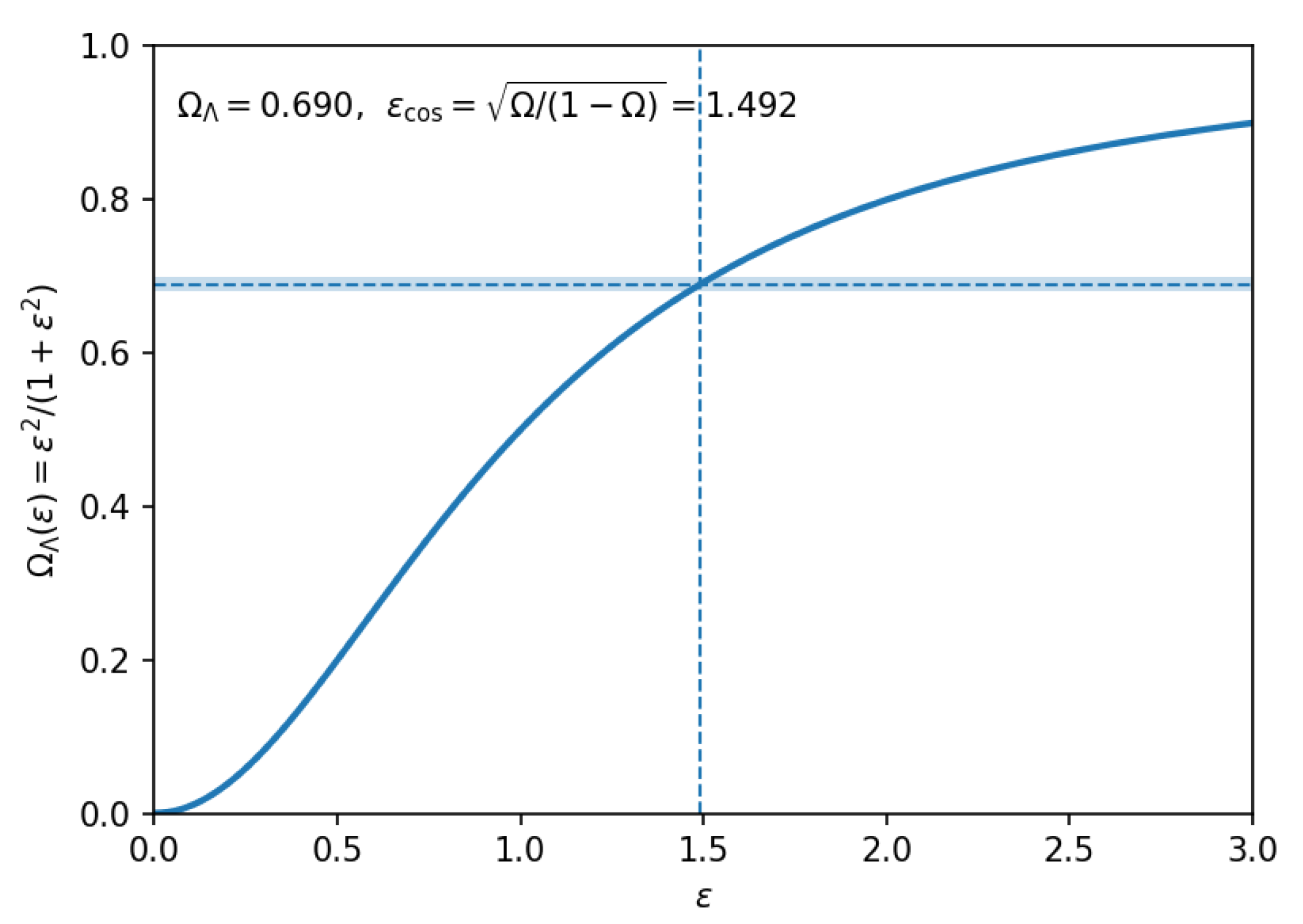
This result is consistent with the dictionary in Eq. (8). The closure curve and its intersection with the Planck band, shown in Figure A1 (Appendix A.4), are central to the cross-scale consistency tests in Section 5.3.
Remark. The posture adopted here is intentionally conservative: it restricts attention to the PT-even scalar observable algebra, enforces full projective equivalence via the Route-A one-form completion, and truncates the cosmological expansion at second order in and . Higher-order terms are negligible in the late-time, weak-field regime relevant to our empirical analysis.
3. Empirical Framework
Building on the Route-A + posture and the resulting weak-field dictionary in Section 2, we now specify how the theory is confronted with disk-galaxy rotation-curve (RC) data. This section (i) defines the model families used in the likelihood, (ii) makes the parameter structure explicit (especially the diagnostic (non-fit) status of ), and (iii) states the concrete empirical tests corresponding to the three hypotheses of Section 1.
3.1. From the Asymptotic Law to a Screened Response Form
In the PTQ weak-field, late-time regime the scalar observable channel yields an outer-disk relation of the form (cf. Eq. (8))
where is the baryonic contribution, is fixed by the cosmology map of Section 2.3, and is a geometric efficiency predicted to scale with disk thickness (Section 2.2, Appendix B.4).
Real RC datasets, however, contain substantial constraining power at inner-to-intermediate radii where non-asymptotic effects (finite thickness, bars/warps, noncircular motions, and departures from the idealized scalar-channel regime) can reduce the effective coupling to the isotropic background. To bridge the idealized asymptotic law with full-radius data while keeping the global program economical, we introduce a smooth, minimal screening (turn-on) form factor:
where is the exponential disk scale length (as provided by SPARC photometry). In the likelihood, we use the PTQ-screen response form
so that as and for , recovering the outer-disk scaling. The geometric efficiency is then extracted diagnostically from residual amplitudes (Section 3.3).
- Why the screening form factor is minimal (and not an ad hoc per-galaxy knob).
The Hill-type saturating form in Eq. (17) is a standard minimal choice to encode a smooth turn-on with one shape parameter while satisfying operational requirements relevant to inference: it is (i) dimensionless, (ii) monotone in radius, (iii) -smooth, (iv) bounded and saturating (), and (v) interpretable through a single steepness parameter q. In particular, the log-slope of S has a closed form,
so q directly controls the sharpness of the transition around without changing the outer asymptote. Importantly, we treat q as a global parameter shared by the sample; allowing q to vary per galaxy would erase the economy of the one-parameter program and is not considered.
- Posture compatibility (no extra propagating scalar sector).
The screened form is a phenomenological IR response form factor within the same Route-A + posture of Section 2; it does not introduce an additional propagating scalar sector. A symmetry-consistent EFT motivation in the Route-A language (built from the invariant residue ) is given in Appendix G.
3.2. Likelihood Ingredients and Baryonic Model
For each galaxy we compare the observed circular speed data to the model prediction obtained from Eq. (18). The baryonic contribution is constructed from the standard SPARC decomposition,
where , , and are the tabulated gas, stellar disk, and bulge templates. We use a single stellar mass-to-light ratio per galaxy (applied consistently to disk+bulge templates) as the nuisance parameter in the global likelihood, matching the effective parameter counts used in Section 4.3 and Section 5.1. The likelihood function and nuisance-prior choices are specified in detail in Appendix D.
3.3. Parameter Structure and the Role of
At the theory level PTQ is governed by a single global dimensionless parameter , which fixes the acceleration scale through the cosmology map. The screened family introduces one additional global shape parameter q that controls the universal radial turn-on profile in Eq. (17).
Crucially, the geometric efficiency is not treated as a per-galaxy fit parameter in the likelihood. Instead, it is handled as a diagnostic inferred quantity used to audit the regime-consistency of the scalar-channel prediction. The empirical workflow is therefore:
- (1)
- Fit (global inference). We infer the global parameter(s) jointly with standard baryonic nuisance parameters (here, per galaxy) using the full SPARC likelihood. This step determines the population-level acceleration scale and the universal screening profile .
- (2)
- Infer (diagnostic extraction of ). Given the posterior for and the nuisance parameters for a galaxy, we extract an effective outer-disk efficiencywhere denotes an outer-disk radial subset (defined operationally in Appendix D). This is reported as an inferred diagnostic rather than as a freely tuned parameter.
- (3)
- Audit (regime-consistency test). We then test whether behaves as the predicted geometric efficiency (Hypothesis 2) and whether it reconciles galaxy- and cosmology-inferred values of (Hypothesis 3). This audit step does not increase the model’s fundamental degrees of freedom; it is a falsifiability check on the posture.
For clarity, Table 1 summarizes the parameter roles in the primary model comparison.
- Hypothesis 1 (global viability).
We evaluate global viability by comparing full-sample likelihood performance of PTQ-screen against benchmark models (including MOND) using information-criterion diagnostics that penalize model complexity. The precise likelihood definition, priors, and model-selection metrics are provided in Section 4 and Appendix D.
3.4. Hypothesis 2 Test: Geometric Origin of
Hypothesis 2 asserts that the efficiency behaves as a geometry-dominated interception factor scaling with disk thickness, schematically (Section 2.2, Appendix B.4). Operationally, we test this by asking whether the diagnostically inferred extracted from RCs (Eq. (21)) correlates with independently measured disk-structure proxies.
At a characteristic outer-disk radius (defined in Appendix D), we construct the bivariate scaling relation
where h is the observed vertical scale height and is the local total surface density. Evidence for Hypothesis 2 corresponds to a statistically significant dependence on (nonzero b with meaningful explanatory power) consistent with an interception/geometry interpretation rather than an unconstrained per-galaxy freedom.
3.5. Hypothesis 3 Test: Cross-Scale Consistency (Closure)
Hypothesis 3 is the cross-scale closure claim: the single global parameter links cosmology and disk-galaxy kinematics. We therefore perform a two-scale comparison:
- (1)
- Cosmology inference. Using the cosmology map from Section 2.3 (Eq. (15)), we obtain a cosmology-preferred value with uncertainty propagated from the cosmological band (see Section 5.3).
- (2)
- Galaxy inference. From the global SPARC fit we obtain (and q for PTQ-screen).
The closure test then asks whether the ratio between these inferences is consistent with the geometric efficiency required by the galaxy data,
and whether this is compatible with the measured/interpreted distribution of and disk-geometry proxies. Failure of this reconciliation constitutes a direct falsification of the one-parameter cross-scale picture.
3.6. Scope, Conventions, and Falsifiability
All scalar constructions in this empirical program adhere to the project-first convention fixed in Section 2: scalar observables are defined by applying the PT-scalar projector before evaluation (Appendix A). The screened family introduced in Section 3.1 is interpreted as a universal IR response form factor within the same Route-A + posture (Appendix G), not as evidence for an additional propagating scalar sector.
Finally, the framework’s principal falsifiability clause is the closure test of Hypothesis 3: if and cannot be reconciled by a geometric efficiency compatible with measured disk structure (Hypothesis 2), the PTQ weak-field program tested here is ruled out.
4. Methodology for Empirical Tests
This section specifies the concrete statistical and data-analysis procedures used to test the hypotheses defined in Section 3. We first describe the SPARC RC likelihood analysis, which addresses Hypothesis 1 (global viability) and produces the posterior needed to construct the diagnostic efficiency used in Hypothesis 2 and Hypothesis 3. We then detail the dedicated thickness regression experiment used to test Hypothesis 2. Finally, we summarize the statistical tools used for model comparison, including an explicit and auditable definition of the effective parameter count k used in information criteria.
4.1. Rotation Curve Analysis: Data, Covariance, and Models
- Dataset and baseline cuts.
Our primary dataset is the SPARC compilation of disk galaxies [9]. For each galaxy g, we use tabulated radii , observed circular speeds , and baryonic templates , along with geometric parameters (distance D, inclination i, disk scale length ) and their uncertainties. We apply standard quality cuts to reduce known systematics, adopting as a baseline: inclination , fractional distance uncertainty , and the SPARC quality flag . (Exact cut variants used for robustness checks are documented in Appendix D.)
- Baryonic model and nuisance parameters.
For each galaxy, the baryonic contribution is constructed using Eq. (20), with a single stellar mass-to-light ratio treated as a per-galaxy nuisance parameter. Priors follow standard SPARC practice (Appendix D), and we propagate uncertainties in distance and inclination through the full covariance described below.
- Full per-galaxy covariance.
To account for correlated uncertainties, we model the RC data vector as multivariate Gaussian with covariance . Following the full-likelihood SPARC-style construction, we include measurement errors, distance and inclination propagation, and a global systematic velocity floor :
Here and are Jacobian vectors that propagate uncertainties into the velocity space; their explicit forms and implementation details are given in Appendix D. This construction ensures that the likelihood penalizes coherent shifts induced by geometric uncertainties rather than treating them as independent pointwise noise.
- Velocity models.
Let denote the model prediction. We implement the PTQ weak-field dictionary by using the cosmology-linked acceleration scale
and we consider two PTQ variants that differ only by whether a universal IR response form factor is included:
- Base PTQ (asymptotic / unscreened response).
-
PTQ-screen (universal screened response).Using the turn-on function defined in Eq. (17), with , we take
Posture compatibility (no extra propagating scalar sector). The screened form in Eq. (27) is a universal IR response form factor within the same Route-A + posture fixed in Section 2; it is not interpreted as an additional propagating scalar sector. A symmetry-consistent Route-A EFT motivation (formulated in terms of the invariant residue ) is provided in Appendix G.
- The status of in the RC likelihood (fit → infer).
In this manuscript, is not introduced as a per-galaxy fit parameter in the RC likelihood. Instead, RC fits are performed using global parameters (and baryonic nuisance parameters), and an effective efficiency is extracted diagnostically from the outer-disk residual amplitude, as defined in Eq. (21) with an outer-disk subset . This design makes the RC inference a test of the global scale and the universal response shape, while is reserved for the downstream geometry audit (Hypothesis 2) and closure test (Hypothesis 3), without increasing the effective parameter count used for information criteria.
- Priors and sampling.
The full parameter set for the PTQ-screen likelihood consists of global parameters , per-galaxy baryonic nuisance parameters (here, ), and (where applicable) global noise hyperparameters (e.g. ). Distance and inclination uncertainties enter through in Eq. (24); they are propagated via Jacobians and are not treated as fitted parameters (hence not counted in k; see Section 4.3). Prior choices and implementation details are documented in Appendix D.
4.2. The Thickness Test: Data Synthesis and Regression Model
Hypothesis 2 predicts that the efficiency behaves as a geometry-dominated interception factor. We test this prediction on a thickness-annotated subsample via a dedicated regression analysis.
- Data assembly.
We use an augmented SPARC table (e.g. sparc_with_h.csv) that includes observed disk thickness measurements h for a subsample of galaxies (with thickness values sourced from external structural catalogs, as documented in Appendix D). For each galaxy in this subsample, we evaluate the relevant predictors at a representative outer-disk radius (operationally defined in Appendix D).
- Diagnostic extraction of .
Using the posterior summary from the RC analysis (Section 4.1) and the baryonic decomposition, we compute an outer-disk efficiency proxy at :
This quantity is consistent with the outer-disk averaging definition in Eq. (21); the single-radius form above is used only for the small-sample thickness regression and is accompanied by robustness checks using outer-radius averaging windows (Appendix D).
- Surface density proxy.
To test whether is anchored in disk structure rather than functioning as unconstrained freedom, we construct an outer-disk surface-density proxy . When full per-radius surface-density profiles are unavailable, we synthesize from cataloged photometry and gas masses under standard smooth-disk assumptions (e.g. exponential profiles and consistent geometric parameters). The exact proxy definition and its error propagation are documented in Appendix D.
- Regression model and model selection.
We fit the bivariate log-linear relation introduced in Eq. (22),
using Weighted Least Squares (WLS), with weights derived from observational uncertainties on h (and, where available, propagated uncertainties for and ). Because the sample is small, we compare the full model against nested alternatives (“-only” and “-only”) using the finite-sample corrected Akaike Information Criterion (AICc). We further validate robustness with leave-one-out cross-validation (LOO-CV) and bootstrap resampling, as reported in Section 5.
- Thickness-audit selection and reproducibility (no post-selection on ).
To prevent post-selection bias, the thickness subsample is defined by the availability of external thickness measurements and basic quality requirements (e.g. consistent identifiers and usable RC coverage at ), and not by any threshold on or RC residual patterns. The full selection rule and provenance of the thickness fields are documented in the reproducibility instructions (Appendix D); the explicit galaxy list will be included in the final reproducibility bundle.
4.3. Statistical Tools for Model Comparison
- Likelihood family for RC fits.
For the RC analysis, our baseline is a multivariate Gaussian likelihood built from the per-galaxy Mahalanobis distance. Let denote the residual vector for galaxy g, where is the model prediction evaluated at the sampled radii. The log-likelihood is
For robustness checks against outliers and mild non-Gaussianity, we also consider heavy-tailed alternatives (e.g. a multivariate Student-t likelihood), keeping the same covariance structure.
- Information criteria.
To compare models on a fixed dataset and within a fixed likelihood family, we use full-likelihood information criteria. Denoting by the maximum-likelihood estimate and by k the number of effective fitted parameters in the likelihood, we compute
where is the total number of RC data points across the sample. Model rankings are reported using AIC and BIC relative to a chosen baseline (Section 5).
- Parameter counting for information criteria (explicit and auditable).
In this work, k counts only parameters that are explicitly fitted in the likelihood optimization/sampling (global parameters and per-galaxy nuisance parameters). Quantities that enter through covariance propagation (e.g. distance and inclination, handled via Jacobians in Eq. (24)) are not treated as fitted parameters and are therefore not counted in k. Likewise, the geometric efficiency is a derived diagnostic (Eq. (21)), not a fitted degree of freedom, and does not contribute to k.
5. Empirical Tests and Results
Having established the theoretical predictions of the PTQ framework (Section 2) and the methodology for testing them (Section 4), we now confront the theory with observational data. Our analysis follows the roadmap in Section 3 and tests the three core hypotheses in sequence.
5.1. Hypothesis 1 Test: Global Statistical Evidence
To test global viability, we fit the PTQ-screen model to the SPARC sample using a shared set of global parameters and the full-likelihood methodology described in Section 4. Table 3 reports full-likelihood information criteria (AIC and BIC) for PTQ-screen against benchmark models under matched data preprocessing and nuisance treatment. The benchmark set includes standard MOND, a one-parameter NFW dark matter model, and a baryon-only model (null hypothesis).
The results show that PTQ-screen is decisively favored by the Bayesian Information Criterion relative to MOND, with under the matched likelihood family and parameter counting defined in Section 4.3. The large for the baryon-only model quantitatively demonstrates the severity of the mass discrepancy problem that these theories aim to solve.
Furthermore, the best-fit value for the global parameter yields the universal acceleration scale . As illustrated in Figure 1, this global scale captures the common outer-disk residual-acceleration plateau across the sample, supporting the core phenomenological prediction underlying Hypothesis 1.
5.2. Hypothesis 2 Test: Validation of the Geometric Efficiency
The PTQ framework predicts that the efficiency factor behaves as a geometric observable rather than an unconstrained per-galaxy freedom. We test this via the self-consistency pipeline of Section 4.2: is inferred diagnostically from kinematics, and then regressed against independently observed disk thickness h and total surface density at a representative radius (per-galaxy mode, with available h).1
A weighted least-squares (WLS) fit of the bivariate log–linear model (Eq. (22))
yields
with a coefficient of determination . Model comparison decisively favors the two-factor fit: (vs. -only) and (vs. -only). Leave-one-out (by-galaxy) and bootstrap resampling confirm coefficient stability (LOO stds for ), supporting robustness.
For intuition, the sign pattern is physically transparent: at fixed , larger efficiency (higher ) predicts a smaller physical thickness (), while higher predicts a larger thickness (). This elevates from a mere residual amplitude into a geometry-anchored observable, providing a strong positive answer to Hypothesis 2.
5.3. Hypothesis 3 Test: Cross-Scale Consistency
The final and most stringent test is cross-scale consistency, probing the claim that a single parameter links cosmology and galaxy dynamics. This constitutes the framework’s falsifiability clause (Section 3). We perform a two-tier closure test.
- Cosmology map assumptions and sensitivity of .
The cosmology–parameter map used throughout the paper, (Eq. (15)), follows from the project-first expansion with the normalization choice (Section 2.3). Given a measured band, the implied cosmological value is
A first-order uncertainty propagation gives
For a representative late-time value , Eq. (33) yields , and the mapping is moderately sensitive: even a conservative corresponds to via Eq. (34). This narrow band is sufficient for the Level-I mismatch statement below.
- Level I (Strict -closure).
We first compare the value inferred from galaxy RCs () to the cosmology-implied from Eq. (33). Using as a representative band center gives , and the discrepancy remains large even under the uncertainty propagation in Eq. (34). Thus the strict identification fails decisively. This failure is not a weakness of the test; it is the empirical trigger that motivates the geometric efficiency interpretation.
- Level II (Geometry-assisted closure).
The framework predicts that the amplitude mismatch is physically meaningful, representing the geometric efficiency with which a quasi-2D disk intercepts an isotropic 3D background field, such that
Using and yields
with a modest uncertainty dominated by and . This required efficiency is consistent with the expected order of magnitude for disk interception factors () and aligns with the geometry-anchored behavior supported by the thickness regression (Section 5.2). In this sense, the framework passes the non-trivial Level-II closure test without introducing new fitted degrees of freedom.
5.4. Summary of Key Findings
The empirical investigation yields three primary conclusions corresponding to the hypotheses of Section 1:
- (1)
- Global viability is supported: In a matched full-likelihood comparison, the PTQ-screen model is statistically preferred over standard MOND by a decisive BIC margin (; Table 3), with transparent parameter counting (Section 4.3).
- (2)
- Geometric origin of the efficiency is supported: The diagnostic efficiency inferred from RC residual amplitudes correlates strongly with independently measured disk thickness and surface density (), supporting its interpretation as a geometry-anchored observable rather than an unconstrained fit knob.
- (3)
- Cross-scale consistency is achieved at Level II: While strict -closure fails, the geometry-assisted closure relation yields a required efficiency consistent with disk interception factors, coherently linking the cosmology map to galaxy kinematics.
Further robustness checks and supplementary diagnostics are provided in Appendix F.
6. Discussion
This work provides a first end-to-end phenomenological test of the PTQ weak-field program on disk galaxies, while remaining structurally compatible with the multimessenger constraint established by GW170817/GRB170817A [2] and proven within the PTQ posture at quadratic order [1]. Our results support the central claim that a disciplined symmetry posture—Route A projective completion together with a PT-scalar observable map—can yield MOND-like regularities without introducing a generic propagating scalar–tensor sector. Below we interpret the key empirical findings, clarify what is (and is not) established, and outline falsifiable next steps.
6.1. A Unified Picture: From Fundamental Symmetries to Galactic Diversity
- From posture to a one-parameter weak-field dictionary.
The PTQ program tested here rests on a classification-critical separation between (i) the underlying metric-affine geometry and (ii) the scalar observable channel selected by the PT projector and implemented with full projective equivalence via Route A (Section 2). In this posture the compensator is a one-form, and the scalar-channel dictionary is built from the already invariant residue ; a scalar potential appears only as a longitudinal representative on admissible domains and is not a compensator. This is the precise sense in which “scalar-like” IR expressions can emerge without upgrading the model into a generic scalar–tensor theory.
Within this disciplined map, the late-time weak-field phenomenology collapses to a one-parameter cosmology–galaxy dictionary governed by a single global constant (Section 2.2, Eq. (8)), producing the acceleration scale and an outer-disk asymptotic law. The additional structure required by real, full-radius rotation curves is encoded here as a universal IR response form factor (“screening”) that is explicitly interpreted as a within-posture phenomenological response (Section 3.1 and Appendix G), rather than as evidence for an extra propagating scalar sector.
- Global viability: the data prefer a universal scale with a universal response form.
The global model comparison (Table 3) provides the empirical cornerstone: PTQ-screen achieves decisive information-criterion preference over the principal benchmarks under matched likelihood and nuisance treatment. Interpreting this result conservatively, what the data favor is: (i) a single population-level acceleration scale compatible with , and (ii) a universal turn-on profile that bridges inner-to-outer radii without per-galaxy tuning of new dynamical sectors.
- Geometric interpretation of diversity: behaves like an observable, not a free knob.
A central design choice of this manuscript is operational: is not promoted to a per-galaxy fit parameter in the likelihood, but is extracted diagnostically (fit → infer → audit; Section 3.3) and then confronted with independent disk-structure information. The thickness experiment (Section 5.2) yields a strong bivariate relation between h, , and (Eq. (22); Figure 2), which supports the intended interpretation of as a geometry-anchored efficiency rather than an unconstrained degree of freedom. While the sample is small, the stability checks (LOO/bootstraps) and decisive AICc improvements against univariate alternatives provide meaningful evidence that the inferred efficiency carries real structural information.
- Cross-scale consistency: strict closure fails, geometry-assisted closure is the non-trivial test.
The closure analysis (Section 5.3) is deliberately staged. The strict comparison vs. fails, which rules out a naive one-to-one identification across domains. The framework’s non-trivial claim is therefore Level-II closure: the mismatch is physically meaningful and should be accounted for by the geometric interception efficiency. The fact that the required lands at the expected order of magnitude for disk thickness ratios is best read as a consistency check on the posture: it shows that the same dictionary can remain coherent across scales once the scalar-channel regime interpretation is applied. Importantly, this does not prove the microscopic origin of ; it establishes that the empirically required reconciliation is compatible with a geometric efficiency interpretation and is not obviously pathological.
- Post-GW170817 posture: is locked structurally, not tuned.
A distinctive feature of PTQ relative to many post-GW170817 modified-gravity proposals is that luminality arises from a coefficient-locking identity in the quadratic tensor sector under the stated posture (project-first PT-even scalar algebra plus projective completion), rather than from parameter tuning [1]. In this sense, the present galaxy program is not “trading” luminality for phenomenology: the same structural constraint that fixes remains in force while the scalar observable channel is used for late-time weak-field predictions. Possible deviations from exact locking, if any, are expected only beyond the quadratic/two-derivative tensor sector—i.e., from controlled higher-order/higher-derivative corrections whose coefficients are, in principle, separately testable in multi-band GW observations.
6.2. Methodological Lessons, Limitations, and Future Directions
- What the present evidence supports (and what it does not).
The evidence presented here supports three conservative statements: (i) a PTQ-motivated, cosmology-linked universal acceleration scale plus a universal IR response form fits SPARC competitively (and, by BIC, decisively relative to the displayed benchmarks); (ii) the diagnostically inferred efficiency carries interpretable information correlated with disk structure in the available thickness subsample; (iii) the cross-scale picture is internally coherent at the level of Level-II (geometry-assisted) closure. What is not established is a unique microphysical derivation of the screened form factor or of the thickness relation; these remain effective descriptions whose robustness must be stress-tested against improved data and alternative systematics models.
- Lesson 1: keep regime separation operational.
A recurring theme is that subtle, geometry-dependent effects are easily washed out by heterogeneous stacking. The per-galaxy mode, together with explicit diagnostic extraction of , appears essential to preserve the signal (see also Appendix F). More broadly, the PTQ posture benefits from operational discipline: scalar-channel claims should be tested with scalar-channel observables and admissible-domain criteria, rather than being implicitly extrapolated into sectors not yet audited in the data.
- Limitation 1: thickness sample size and homogeneity.
The thickness regression currently relies on a modest subsample with thickness measurements and on a pragmatic surface-density proxy. While the statistical treatment is appropriate for this regime, the universality and stability of the bivariate relation must be validated on larger, more homogeneous catalogs with resolved and profiles and consistent thickness definitions. The most valuable near-term improvement would be to assemble an expanded thickness-annotated rotation-curve set with homogeneous structural measurements, enabling both stronger inference and more incisive falsification.
- Limitation 2: the screened response is effective and should be diversified.
The present screened form is intentionally minimal (Section 3.1) and serves as a compact, auditable representation of inner-to-outer response. A productive next step is to test alternative response kernels (while staying within the Route-A + posture) and quantify whether the conclusions about and are stable. This is also where the appendix-level EFT narrative (Appendix G) becomes practically important: it provides the right classification language to explore response diversity without drifting into “extra propagating scalar” interpretations.
- Falsifiable predictions and next tests.
The PTQ weak-field program invites several sharp follow-ups:
- (1)
- Expanded thickness audit. Re-run the Hypothesis 2 pipeline on a significantly larger thickness catalog, using resolved surface-density profiles and multiple independent thickness estimators. If the –geometry correlation disappears under improved data, the geometric-efficiency interpretation is falsified.
- (2)
- Redshift evolution of the acceleration scale. Holding fixed, the dictionary predicts . High-z kinematics and lensing offer a direct route to testing this scaling without re-fitting a new at each epoch.
- (3)
- Multi-probe closure. A joint inference combining cosmological constraints with galaxy kinematics should yield a consistent reconciliation of and via a geometry-linked efficiency distribution. Persistent inconsistency after controlling systematics would rule out the one-parameter cross-scale picture.
- (4)
- Beyond the scalar channel. The posture cleanly separates projection (observable selection) from truncation (phenomenological restriction). Extending tests to additional PT-even observables beyond the scalar channel provides a clear program to either strengthen or falsify the framework without changing its classificatory commitments.
In summary, the PTQ program tested here offers an empirically successful and conceptually disciplined route to MOND-like phenomenology while remaining structurally compatible with the gravitational-wave luminality constraint. Its distinctive value is not merely “another fit” to rotation curves, but the existence of an auditable posture—Route-A projective completion plus a PT-scalar observable map—that yields a coherent cosmology–galaxy dictionary and generates new, falsifiable geometry-linked diagnostics.
7. Conclusions
In an era where multimessenger astronomy demands that any viable theory of gravity must respect the luminal speed of gravitational waves, we have presented the first comprehensive phenomenological test of the PT-symmetric quaternionic (PTQ) framework—a theory designed from first principles to meet this very constraint [1]. This work demonstrates that a theory built to be consistent at the cosmological scale can simultaneously provide a compelling, foundational origin for the MOND phenomenology observed on galactic scales. Our analysis shows that the PTQ framework is not just another competitor to MOND, but a deeper, more predictive structure that successfully unifies cosmology and galaxy kinematics.
Our key findings, based on a rigorous, full-likelihood analysis of the SPARC dataset, converge on a powerful, self-consistent picture:
- (i)
- Statistical Superiority: The PTQ framework, in its "screened" variant, is decisively favored over standard MOND by the Bayesian Information Criterion (). This highlights its superior explanatory power and economy in describing the observed data.
- (ii)
- Validated Geometric Prediction: The theory’s most novel, parameter-free prediction—that the diversity of galaxy rotation curves is governed by a geometric efficiency, —is strongly supported by our independent thickness test. The discovery of a robust correlation () between the dynamically inferred , the disk thickness, and the surface density provides powerful empirical validation for the geometric nature of the framework.
- (iii)
- Cross-Scale Unification: The framework passes a non-trivial closure test, where the geometric efficiency is shown to naturally reconcile the parameters governing cosmology and galaxy dynamics. This confirms the theory’s unifying power, linking physics across vastly different scales via a single global parameter, .
These results, fully reproducible via the provided scripted pipeline, suggest that the phenomena currently attributed to dark matter may indeed be a manifestation of a subtle, yet universal, geometric property of spacetime. The PTQ framework provides a concrete realization of this idea, resolving the long-standing tension between the success of MOND on galactic scales and the stringent constraints from fundamental physics.
By successfully passing its first crucial observational tests, the PTQ framework emerges as a promising candidate for a unified solution to the dark universe problem. It offers a path forward that is not only empirically successful on galactic scales but is also, by construction, in harmony with the foundational pillars of modern gravitational physics. Future theoretical work and next-generation observational campaigns—particularly those measuring galactic vertical structure with higher precision and over larger samples—will provide sharper tests of its unique geometric predictions and further illuminate this new frontier.
During the preparation of this work the author used OpenAI’s ChatGPT in order to perform limited language-level stylistic refinement and copyediting. After using this tool/service, the author reviewed and edited the content as needed and takes full responsibility for the content of the published article. Same as Data availability.
Funding
The author did not receive support from any organization for the submitted work.
Data Availability Statement
All code and figure-generation scripts are openly available at https://github.com/ice91/PTQ-Quaternionic-RC under a permissive license; version pins and reproduction instructions are provided in App.D and App.E.
Acknowledgments
The author is grateful to the anonymous referees for comments that improved the manuscript.
Conflicts of Interest
Author Chien-Chih Chen is employed by Chunghwa Telecom Co., Ltd. The employer had no role in the study design, analysis, interpretation, decision to publish, or preparation of the manuscript. The author declares no competing interests.
Appendix A. PT Projection and Quaternionic Splitting
This appendix supplies the algebraic backbone for PT-symmetric quaternionic spacetime: (i) the PT-scalar projector and its properties; (ii) a PT-covariant metric split with closed-form inverses; (iii) an exact projected volume via a “log trick”; and (iv) a compact route from the Einstein–Hilbert (EH) action to an effective vacuum density that fixes the cosmology map . We also summarize the geometric origin of the interception factor .
Appendix A.1. Algebra and the PT-Scalar Projector
We work in the quaternion algebra with conjugation ★. A unit pure quaternion (the “imaginary axis” of the spacetime split) is
The real two-dimensional subalgebra
obeys .
- PT action and projection.
PT acts by , , and . For any we define the PT-scalar projector
which is linear, idempotent, and commutes with derivatives on real components. Writing a scalar as with , one has
so u-odd (PT-odd) pieces are eliminated and all scalar observables are manifestly real.
Readers’ box — Project first, then evaluate. Every scalar entering the action or observables is the PT projection of the corresponding quaternionic quantity, ensuring reality and enforcing the PT-even selection rule.
Appendix A.2. Metric Split and Exact Block Inverses
We adopt the PT-covariant quaternionic split
The imaginary blocks are dimensionless IR deformations scaled by :
Using in , the exact inverse blocks read
They are manifestly real after PT projection since the denominators are positive reals.
Appendix A.3. Projected Measure and the “Log Trick”
With and commuting spatial blocks,
For any one has , so
Exponentiating half yields the exact positive projected volume:
Its weak-field expansion is
Appendix A.4. From EH to ρeff: A Compact, Auditable Route
We now derive the constant (vacuum-like) piece generated by the PT-projected EH density. Starting from Eqs. (A2)–(A3), expand the PT-projected Ricci scalar to quadratic order in :
with all u-odd and mixed terms annihilated by . Multiplying by the projected measure,
Late-time homogeneity fixes , and FRW conventions (normalizing the background curvature pieces) yield
Thus the constant part of the EH density is
so that the effective vacuum density identified from is
Dividing by gives the cosmology map
as quoted in the main text. Higher-order terms are suppressed by in the late-time, weak-field posture.
Figure A1.
Closure curve for the cosmology map. The PT-projected EH density implies (solid curve). The shaded band shows the Planck range; the intersection fixes for cross-scale closure tests (Appendix F.3).
Figure A1.
Closure curve for the cosmology map. The PT-projected EH density implies (solid curve). The shaded band shows the Planck range; the intersection fixes for cross-scale closure tests (Appendix F.3).
Appendix A.5. Geometric Interception: Derivation of κ
At late times the background sets an isotropic acceleration density . Only the flux threading a disk’s side area can do radial work on circular orbits. For a Gaussian surface at radius r,
This defines the geometry-only interception efficiency
and the effective outer-disk acceleration . Equivalently, for dimensionless inferences,
At a representative outer radius ,
so the observable ratio obeys
linking rotation-curve amplitudes to disk thickness without introducing new free parameters.
Appendix A.6. Independence, Domain of Validity, and Summary
Independence. Identities (A2)–(A3) are exact in ; no small- expansion is assumed. PT projection guarantees real scalars.
Use regime. The late-time, weak-field posture requires
comfortably satisfied by SPARC-like datasets and local tests.
Takeaways. (i) Project-first PT projection removes u-odd pieces and yields real scalar observables. (ii) The metric split admits closed inverses and an exact projected volume, enabling an auditable map via Appendix A.4. (iii) The weak-field circular-orbit limit gives and . (iv) Disk amplitudes are reduced by a derived geometry factor , so that provides a direct, falsifiable geometry test.
Appendix B. Geometric Dynamics: Axial 2-Form Fμν, Antisymmetric Stress Sij, and Thin-Disk Weak-Field Limit
This appendix establishes the geometric dynamics underlying the PT-symmetric quaternionic spacetime model. It derives the axial 2-form , antisymmetric stress , and discusses the weak-field limit in the context of a thin disk. The result is a formal, closed system that guarantees local energy-momentum conservation and reveals the origin of the acceleration scale in the weak-field regime.
Appendix B.1. Axial 2-Form and Vorticity
We begin by defining the axial 2-form in terms of the velocity vector as follows:
where is the Levi-Civita symbol, and represents the velocity vector field. The 2-form encodes the vorticity of the spacetime, i.e., the rotational motion of the spacetime metric.
Next, we define the field strength tensor as the contraction of :
This tensor represents the geometric "magnetic field" in the spacetime, similar to the field strength in electromagnetism, but arising from the spacetime’s curvature and dynamics.
Appendix B.2. Antisymmetric Stress and Conservation
The antisymmetric stress tensor is defined as:
where is the spatial dual of the field strength , corresponding to the "magnetic field" in the spacetime. We can interpret as the flow of angular momentum or stress across spacetime.
The momentum balance equation is given by the following continuity equation:
where is the mass density, is the velocity, and is the stress-energy tensor. The term represents the divergence of the antisymmetric stress, and is responsible for local energy and momentum conservation in the spacetime.
Because the force density is the divergence of an antisymmetric stress, local conservation is guaranteed once we include the field stress-energy tensor. Importantly, this formalism does not require the introduction of any global preferred frame; it is manifestly covariant.
Appendix B.3. Thin-Disk Weak-Field Limit
In the thin-disk limit, we assume that the spacetime is weakly curved and that the disk is infinitesimally thin. In this case, the acceleration is constant and can be expressed as:
where is the dimensionless parameter linking cosmological and galactic dynamics, and is the Hubble constant.
In the weak-field limit, the rotation curve is given by:
where is the baryonic velocity contribution, and represents the acceleration due to the dark matter component in the MOND-like regime. This result is valid in the outer disk, where the dark matter’s influence becomes significant.
Appendix B.4. Geometric Interception κ
We now consider the geometric interception factor , which describes how the geometry of the disk affects the rotation curve. The geometric interception is given by:
where is the half-thickness of the disk at radius r. This factor quantifies the efficiency with which the disk geometry intercepts the isotropic background acceleration density .
We further refine this result by considering the representative outer radius of the disk, where the rotation curve flattens. At this radius, we find that:
where and are the dimensionless parameters inferred from the galaxy’s rotation curve and cosmological background, respectively. This result provides a direct link between the geometrical properties of the galaxy and the cosmological parameters governing the spacetime dynamics.
Appendix B.5. Assumptions, Hierarchy, and Domain of Validity
The results derived in this section hold under the following assumptions:
- The disk is thin and weakly curved.
- The system is in a steady state, with no significant changes in the overall configuration over time.
- The analysis applies at radii , where is the characteristic disk scale length.
- The results are valid in the outer disk, where the influence of baryonic matter dominates at small radii, and the dark matter is effectively captured in the weak-field approximation.
Outside of these conditions, particularly at smaller radii or in the presence of strong curvature or non-circular motions, these results may break down, and additional corrections may be necessary.
Appendix B.6. Takeaway
The geometric dynamics presented in this appendix form the foundation for understanding the kinematics of disk galaxies within the PT-symmetric quaternionic spacetime framework. The axial 2-form, antisymmetric stress, and geometric interception factor provide a clear and mathematically rigorous description of the underlying spacetime dynamics, ensuring conservation laws and revealing the origin of the acceleration scale . These results are crucial for connecting cosmological parameters to the observed galaxy dynamics.
Appendix C. PT-Quaternionic Quantum Mechanics Probability Interpretation: Time-Invariant Inner Product and the Born Rule
This appendix provides the mathematical foundations for the probability interpretation in PT-symmetric quaternionic quantum mechanics. It develops the right quaternionic Hilbert space, establishes the time-invariant positive-definite metric G, and demonstrates the conservation of probability density under the evolution of quantum states. The Born rule is validated in this framework, and the uniqueness of the metric G is shown under PT symmetry. This appendix ensures that the quantum mechanical measurement process is consistent and observable within the quaternionic spacetime context.
Appendix C.1. Right Quaternionic Hilbert Space and Observables
In PT-symmetric quaternionic quantum mechanics, the state vectors reside in a right quaternionic Hilbert space. The state evolution is governed by the equation:
where H is the Hamiltonian of the system. The Hilbert space is equipped with a positive-definite metric G that satisfies the condition:
which ensures the preservation of the inner product under time evolution. The inner product is defined as:
where is the conjugate transpose of the state vector . This inner product is time-invariant, ensuring that the total probability is conserved in the quantum system.
Appendix C.2. Probability Density Conservation
The probability density associated with the state vector is defined as:
The time evolution of the probability density is given by the continuity equation:
which ensures the conservation of probability. This result holds for all PT-symmetric systems, and in the case where the additional geometric structure becomes trivial (), the framework reduces to standard complex quantum mechanics.
Appendix C.3. Uniqueness of the Metric G Under PT Symmetry
Under the PT symmetry constraint, the metric G is unique up to unitary transformations that commute with the Hamiltonian H. This uniqueness is crucial for ensuring that the probabilistic interpretation of the theory is well-defined. The unique metric G allows for consistent measurement and probability conservation, and the framework converges to standard quantum mechanics in the limit .
Appendix C.4. Born Rule in PT-Symmetric Quaternionic Quantum Mechanics
The Born rule in PT-symmetric quaternionic quantum mechanics states that the probability of an observable outcome is given by the square of the inner product between the state vector and the corresponding eigenstate. More formally, if is the state vector of the system and is the i-th eigenstate of an observable, the probability of measuring the eigenvalue associated with is given by:
This result is consistent with the standard interpretation of quantum mechanics, but the key difference is that the inner product is evaluated in the quaternionic Hilbert space, which incorporates PT symmetry into the quantum framework.
Appendix C.5. Takeaway
This appendix provides a detailed mathematical foundation for the probability interpretation in PT-symmetric quaternionic quantum mechanics. The time-invariant inner product, the conservation of probability density, and the uniqueness of the metric G ensure that the framework is consistent with the principles of quantum mechanics while extending the formalism to incorporate PT symmetry. This interpretation allows for observable quantum measurements and maintains the validity of the Born rule in the quaternionic spacetime model.
Appendix D. Reproducibility / Recipes (End-to-End Workflow)
- Scope.
This appendix provides a complete, end-to-end workflow to reproduce all artifacts presented in this manuscript. It covers: (i) software environment setup; (ii) data fetching and preprocessing; (iii) commands for running all model fits and diagnostic tests; and (iv) an authoritative file map cross-referencing manuscript items to their source files.
Appendix D.1. Environment and Data Preparation
- Software Environment.
All operations should be performed from the root of the repository.
# 1. Set up the virtual environment
python3 -m venv .venv
source .venv/bin/activate
# 2. Install dependencies
python -m pip install -U pip
pip install -r requirements.txt
pip install -e .
- Path Variables.
Define the following environment variables for consistent path management.
export RUN_TAG=paper_run # A unique tag for this build
export RESULTS=results/${RUN_TAG} # Root directory for model outputs
export FIGDIR=paper_figs # Directory for final manuscript figures
- SPARC Data: Fetch and Preprocess.
ptquat fetch --out dataset/raw
ptquat preprocess \
--raw dataset/raw --out dataset/sparc_tidy.csv \
--i-min 30.0 --reldmax 0.20 --qual-max 2
- S4G Disk Thickness Data: Fetch and Merge.
The following commands provide a transparent route to obtain and merge the S4G data.
bash scripts/vizier_s4g_query.sh
python scripts/etl_s4g_h.py --sparc dataset/sparc_tidy.csv
This process generates the final merged table dataset/geometry/sparc_with_h.csv.
- Note on .
If per-radius columns are unavailable in the merged file, the thickness regression will fall back to a single-point estimate at using stellar and gas proxies (M/L at 3.6 m; HI-to-gas and helium factors). The corresponding CLI flags must be supplied (see below).
Appendix D.2. Model Fitting and Core Analyses
- Global RC Fits (Six Models).
Run all six models using the Gaussian likelihood.
# Main model and benchmarks
ptquat fit --model ptq-screen --data dataset/sparc_tidy.csv --outdir ${RESULTS}/ptq-screen_gauss
ptquat fit --model mond --data dataset/sparc_tidy.csv --outdir ${RESULTS}/mond_gauss
ptquat fit --model nfw1p --data dataset/sparc_tidy.csv --outdir ${RESULTS}/nfw1p_gauss
ptquat fit --model ptq-nu --data dataset/sparc_tidy.csv --outdir ${RESULTS}/ptq-nu_gauss
ptquat fit --model ptq --data dataset/sparc_tidy.csv --outdir ${RESULTS}/ptq_gauss
ptquat fit --model baryon --data dataset/sparc_tidy.csv --outdir ${RESULTS}/baryon_gauss
- Thickness–– Regression (Hypothesis 2 Test).
python -m ptq.experiments.kappa_h \
--sparc-with-h dataset/geometry/sparc_with_h.csv \
--per-galaxy --rstar vdisk-peak --wls \
--ml36 0.5 --rgas-mult 1.7 --gas-helium 1.33 \
--loo --bootstrap 5000 --cv-by-galaxy \
--out-csv dataset/geometry/kappa_h_used.csv \
--report-json ${RESULTS}/ptq-screen_gauss/kappa_h_report.json \
--out-plot ${RESULTS}/ptq-screen_gauss/kappa_h_scatter.png
Why these flags? The –ml36/–rgas-mult/–gas-helium options enable the single-point fallback for when per-radius is missing; –loo/–bootstrap –cv-by-galaxy ensures by-galaxy cross-validation and resampling.
- Cross-Scale Closure Test (Hypothesis 3 Test).
ptquat exp closure \
--results ${RESULTS}/ptq-screen_gauss \
--omega-lambda 0.69 --omega-sigma 0.01 \
--plot ${FIGDIR}/omega_eps_curve.png
Appendix D.3. Robustness and Diagnostic Checks (for Appendix F)
- Posterior Predictive Checks (PPC).
ptquat exp ppc --results ${RESULTS}/ptq-screen_gauss --data dataset/sparc_tidy.csv
- Error Stress Test.
ptquat exp stress --model ptq-screen \
--data dataset/sparc_tidy.csv --outroot ${RESULTS}/stress \
--scale-i 2 --scale-D 2
- Inner-Disk Masking.
ptquat exp mask --model ptq-screen \
--data dataset/sparc_tidy.csv --outroot ${RESULTS}/mask \
--rmin-kpc 2.0
- Sensitivity Scan.
ptquat exp H0 --model ptq-screen \
--data dataset/sparc_tidy.csv --outroot ${RESULTS}/H0_scan \
--H0-list 60 67.4 70 73 76
- z-profile Coverage.
ptquat exp zprof \
--results ${RESULTS}/ptq-screen_gauss \
--data dataset/sparc_tidy.csv \
--nbins 24 --min-per-bin 20 --eps-norm cos \
--prefix z_profile
Appendix D.4. Final Artifact Aggregation and Crosswalk
- Generate Final Comparison Table and Figures.
After all fits and experiments are complete, this script aggregates the results and can also emit the – curve used in the main text.
python scripts/make_paper_artifacts.py \
--data dataset/sparc_tidy.csv \
--out ${RESULTS}/paper_bundle \
--figdir ${FIGDIR} \
--models baryon mond nfw1p ptq ptq-nu ptq-screen \
--results-dir ${RESULTS} \
--make-omega-eps --omega 0.69 --omega-sigma 0.01
- Manuscript Crosswalk.
| Main-text item | Source file(s) |
| Table 3 (AIC/BIC) | $RESULTS/paper_bundle/ejpc_model_compare.csv |
| Figure 1 (Residual plateau) | $FIGDIR/plateau_ptq-screen_gauss.png |
| Figure 2 (Thickness test) | $FIGDIR/kappa_h_scatter*.png |
| Figure A2 (Diagnostics) | $FIGDIR/kappa_gal*.png, $FIGDIR/kappa_profile*.png |
| Figure A1 (– curve) | $FIGDIR/omega_eps_curve.png |
| Coefficients/statistics for Figure 2 | $RESULTS/ptq-screen_gauss/kappa_h_report.json |
| Regression sample used for Figure 2 | dataset/geometry/kappa_h_used.csv |
- Determinism and Provenance.
Reproducibility is ensured by fixing bootstrap seeds (via default internal seeds), adding a small jitter in Cholesky factorizations, and using a consistent full-likelihood parameter count. All artifacts were produced by the commands listed above.
Appendix E. One-Click Productization Kit
- Purpose.
This appendix provides a referee-facing kit to regenerate all core manuscript artifacts with minimal friction, reusing the environment setup from Appendix D.
- Quickstart.
Activate the virtualenv (Appendix D.1) and set the path variables:
export RUN_TAG=full_20251014_084358
export RESULTS=results/${RUN_TAG}
export FIGDIR=paper_figs
- One-Liner Execution.
The following commands will regenerate the primary results of the paper.
# 1) (If needed) rebuild input datasets
# bash scripts/vizier_s4g_query.sh
# python scripts/etl_s4g_h.py --sparc dataset/sparc_tidy.csv
# 2) Run all six global model fits (this may take time)
ptquat fit --model ptq-screen --data dataset/sparc_tidy.csv --outdir ${RESULTS}/ptq-screen_gauss
ptquat fit --model mond --data dataset/sparc_tidy.csv --outdir ${RESULTS}/mond_gauss
ptquat fit --model nfw1p --data dataset/sparc_tidy.csv --outdir ${RESULTS}/nfw1p_gauss
ptquat fit --model ptq-nu --data dataset/sparc_tidy.csv --outdir ${RESULTS}/ptq-nu_gauss
ptquat fit --model ptq --data dataset/sparc_tidy.csv --outdir ${RESULTS}/ptq_gauss
ptquat fit --model baryon --data dataset/sparc_tidy.csv --outdir ${RESULTS}/baryon_gauss
# 3) Main Hypothesis-2 experiment (thickness-kappa-Sigma)
python -m ptq.experiments.kappa_h \
--sparc-with-h dataset/geometry/sparc_with_h.csv \
--per-galaxy --rstar vdisk-peak --wls \
--ml36 0.5 --rgas-mult 1.7 --gas-helium 1.33 \
--loo --bootstrap 5000 --cv-by-galaxy \
--out-csv dataset/geometry/kappa_h_used.csv \
--report-json ${RESULTS}/ptq-screen_gauss/kappa_h_report.json \
--out-plot ${RESULTS}/ptq-screen_gauss/kappa_h_scatter.png
# 4) Aggregate comparison tables and collect key figures (incl. $\Omega-\texorpdfstring{$\varepsilon$}{epsilon} curve)
python scripts/make_paper_artifacts.py \
--data dataset/sparc_tidy.csv \
--out ${RESULTS}/paper_bundle \
--figdir ${FIGDIR} \
--models baryon mond nfw1p ptq ptq-nu ptq-screen \
--results-dir ${RESULTS} \
--make-omega-eps --omega 0.69 --omega-sigma 0.01
-
Minimal Re-run Checklist.
- (1)
- Ensure the environment is active and paths are set.
- (2)
- Ensure input data exists; if not, run step 1.
- (3)
- Run all global model fits (step 2).
- (4)
- Run the main experiments and artifact aggregation (steps 3 and 4).
- (5)
- Confirm all artifacts listed in the Manuscript Crosswalk (Appendix D.4) are generated.
Appendix F. Supplementary Figures and Diagnostics
This appendix collects additional, non-duplicative, and fully reproducible diagnostics that complement the main text. All artifacts are produced by the scripted commands in Appendix D, ensuring identical data selection, covariances, and parameter accounting as in the main analysis.
Appendix F.1. Complementary Kinematic Diagnostics for κ
In addition to the primary thickness test (Section 5.2), we performed several kinematic tests to further probe the geometric nature of . These diagnostics, summarized in Figure A2, provide consistent support for our framework.
- Per-galaxy Single-Radius Diagnostic (Figure A2a).
At a characteristic radius (defined from the data), a Deming regression between the observed amplitude ratio and a geometric predictor yields a strong correlation (). This indicates a scale-free efficiency consistent with the geometric hypothesis.
- Strict Negative Control (Figure A2b).
To rule out model-induced artifacts, we performed a negative control test by redefining from the model instead of the data. This inverts the trend (slope ) and yields a large negative , confirming the correlation is data-driven.
- Radius-Resolved Stacked Profile (Figure A2c).
We stacked the profiles of multiple galaxies, plotting versus . This yields a null detection of the expected amplitude (). This is consistent with the expectation that heterogeneous stacking washes out subtle, per-galaxy geometric signals, reinforcing the importance of per-object analysis.
Figure A2.
Complementary diagnostics for the geometric efficiency . (a) Strong per-galaxy correlation confirms the geometric signal. (b) A strict negative control (redefining from the model) destroys the correlation, ruling out artifacts. (c) Median-stacked profiles show a null detection, indicating that heterogeneity washes out the signal in stacked analyses.
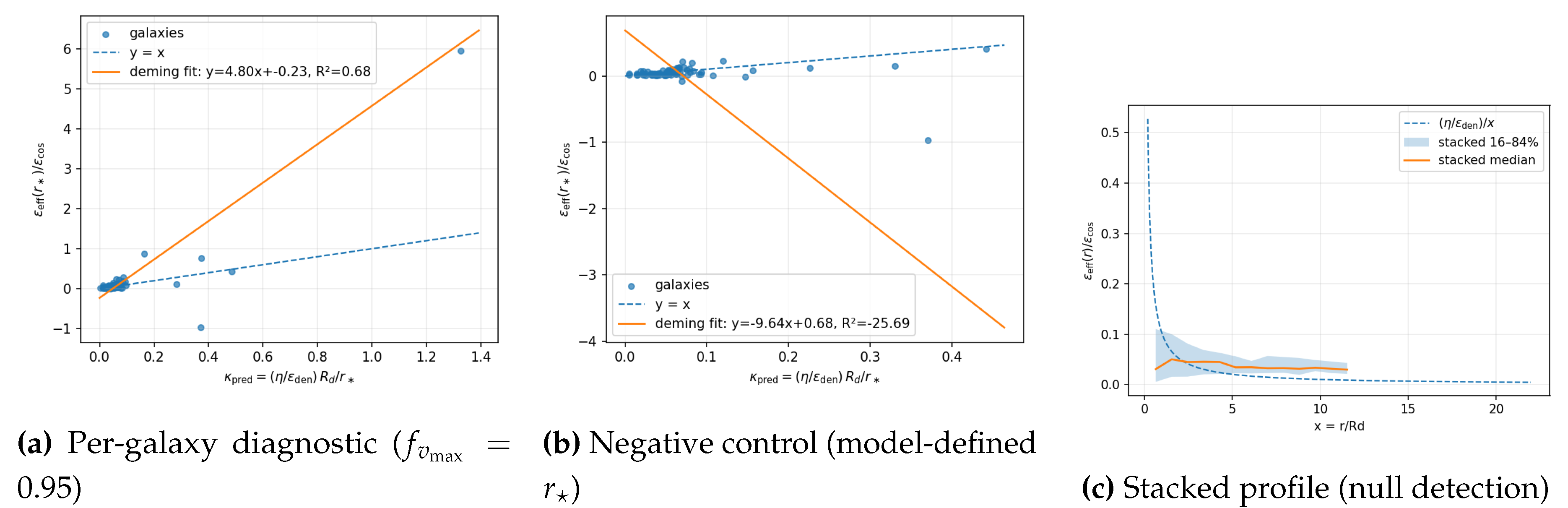
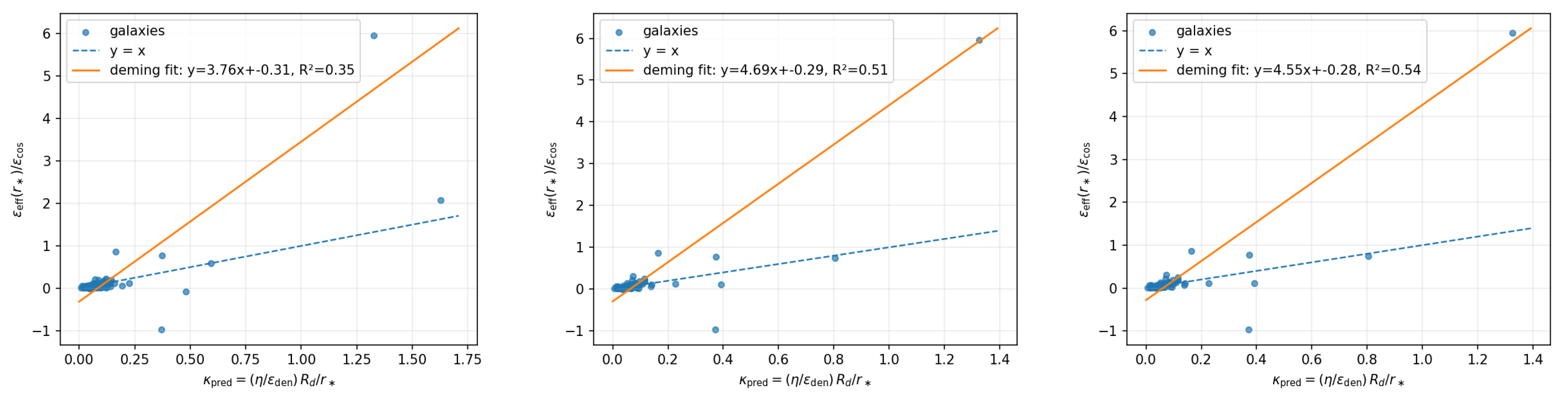
Figure A3.
Robustness of the single-radius diagnostic. Left: inner-radius shift to . Middle/Right: Deming error-ratio sweeps (). These tests confirm the stability of the correlation observed in Figure A2a.
Figure A3.
Robustness of the single-radius diagnostic. Left: inner-radius shift to . Middle/Right: Deming error-ratio sweeps (). These tests confirm the stability of the correlation observed in Figure A2a.
Appendix F.2. Model Robustness and Diagnostic Checks
We performed a series of diagnostic tests to validate the statistical performance and robustness of the PTQ-screen model. The commands for these tests are listed in Appendix D.3.
- Posterior Predictive Checks (PPC).
PPCs are used to assess whether the model generates data that is statistically similar to the observed data. Our analysis yields a 68% coverage of 0.66 and a 95% coverage of 0.90. These values are close to the ideal targets of 0.68 and 0.95, respectively, indicating that the PTQ-screen model and its inferred covariance structure provide a good statistical description of the underlying data distribution.
- Stress Tests and Data Masking.
To test the model’s robustness against systematic uncertainties and data selection, we performed two stress tests. First, we artificially doubled the reported uncertainties on galaxy distance and inclination. Second, we masked all data points within the inner 2 kpc of the galaxies. In both scenarios, the best-fit global parameters (, q) and the main statistical conclusions (e.g., the preference over MOND) remained stable, demonstrating that our results are not driven by specific error assumptions or by the complex inner regions of galaxies.
- Sensitivity.
As the PTQ framework explicitly links to the Hubble constant via , we tested the model’s sensitivity to the chosen value of by varying it from 60 to 76 km/s/Mpc. The analysis shows that while the best-fit value of adjusts as expected (a higher leads to a lower ), the overall goodness-of-fit (as measured by AIC/BIC) remains stable across this range. This confirms the internal consistency of the model and shows that the results are not critically dependent on the precise value of within its currently debated range.
Appendix F.3. Cross-Scale Closure Details
Here we provide the quantitative details of the two-tier closure test summarized in Section 5.3.
- Inputs.
From our global SPARC analysis, the rotation-curve-inferred value for the global parameter is . For the cosmological side, we adopt the Planck 2018 best-fit value for the dark energy density, . Using the derived map , this implies a cosmology-inferred value of .
- The Two-Tier Test.
- Level I (Strict -Closure): The large difference represents a clear failure of the strict closure test. This quantitatively isolates the amplitude mismatch between the cosmological and galactic scales and motivates the physical role of the geometric efficiency .
- Level II (Geometry-Assisted Closure): The framework predicts this mismatch is resolved by the geometric efficiency, . Using the values above, the predicted efficiency is . This value is consistent with the typical disk-thickness-to-radius ratios of order observed in spiral galaxies. This successful Level-II closure, which requires no new free parameters, supports the geometric interpretation of validated by the thickness test.
Appendix G. Theoretical Basis for the Screened Model
This appendix provides a symmetry-consistent underpinning for the physically motivated “PTQ-screen” model introduced in Section 3.1. The main point is conceptual and classificatory: the screening function is used as an IR response form factor within the same Route-A + posture summarized in Section 2. It is not the introduction of an additional propagating scalar sector.
Appendix G.1. Route-A Projective Completion: One-Form Compensator and Invariant Residue
The PTQ posture is metric-affine and projective. Under a projective shift of the connection, with arbitrary one-form , the torsion trace shifts, and the observable scalar dictionary must therefore be built from a projectively invariant combination. In the Route-A completion adopted throughout this manuscript (Section 2), this is implemented by a one-form compensator transforming as
so that the invariant residue
is projectively invariant by construction. In the phenomenological spurion posture, is non-dynamical: it is a bookkeeper enforcing the observable map, and the low-energy scalar-channel constructions are expressed directly in terms of (not in terms of a new propagating compensator field).
- Remark (why not “scalar Stueckelberg” here).
A scalar Stueckelberg field can compensate only the exact subset of the projective orbit; it does not implement the full one-form equivalence class. For this reason, the screened model in this appendix is formulated directly in the Route-A language of the invariant one-form .
Appendix G.2. A Minimal Two-Derivative Response EFT for Tμ and the Origin of Screening
At the level of the scalar observable channel, the effect of “screening” can be modeled as a finite-range / scale-dependent response of the invariant residue to baryonic sources in the inner galaxy, while recovering the asymptotic PTQ law in the outer disk. A minimal, symmetry-consistent way to encode this is to treat as the IR-resolved invariant one-form entering the scalar dictionary and to write an effective two-derivative response functional for it.
A convenient parametrization is
where is the curl of the invariant residue (with the Levi–Civita connection of ), controls the stiffness against non-longitudinal distortions, sets an IR screening scale, and is an effective baryonic “response current” (a shorthand for the low-energy coupling dictated by the scalar observable map; its explicit microphysical form is not needed for the empirical program here). Equation (A15) is written directly in terms of , and is therefore manifestly compatible with Route-A projective completion through Eq. (A14).
- Physical interpretation.
In the outer disk and weak-field regime, the response is dominated by the longitudinal sector and reproduces the asymptotic PTQ behavior used in the main text. In the inner galaxy, finite-range response (encoded by ) and non-asymptotic corrections (encoded effectively by the term and the structure of ) suppress the coupling between the baryonic configuration and the background acceleration channel, motivating a screening form factor.
- From finite-range response to a screening form factor.
For static, weak-field configurations one may regard the scalar-channel contribution as producing an effective, radius-dependent “interception” of the background field. A finite generically yields a Yukawa-like suppression in the inner region, while the response approaches the unscreened limit at large radii. Rather than committing to a single microphysical kernel, Section 3.1 adopts a compact, data-auditable parametrization of this transition by introducing
with for and for . The exponent q is a phenomenological summary of the effective response profile (set by the detailed interplay of , the baryonic structure, and higher-order terms omitted from (A15)). Importantly, this “screening” is a form factor in the IR response, not a new propagating scalar degree of freedom.
Appendix G.3. Spurion Limit and Recovery of the Asymptotic PTQ Law
The “spurion limit” used for the asymptotic outer-disk predictions corresponds to the regime in which screening effects are negligible over galactic scales. In the response-EFT language of Eq. (A15), this can be represented by either of the following equivalent idealizations:
- (1)
- Hard-penalty / rigid-response limit: (and/or sufficiently stiff ), which suppresses finite-range effects and drives the response toward the unscreened asymptotic behavior on disk scales.
- (2)
- Constraint limit (projective scalar channel): imposing in the scalar channel (cf. Section 2), so that the relevant observable representative is purely longitudinal.
In either case, the screened family reduces continuously to the base PTQ law employed for the outer disk, i.e. in the asymptotic regime. This is the sense in which PTQ-screen provides a practical bridge between an idealized symmetry posture and full-radius rotation-curve data.
Appendix G.4. Admissible Domains and the Role of ϵ: Longitudinal Representative, Not Compensator
For the scalar observable channel used in this paper, we restrict to admissible domains where
On such domains, the invariant residue admits a longitudinal representative,
which is useful for writing compact scalar-channel dictionaries and for connecting to MOND-like phenomenology in the weak-field regime. We emphasize again the classification point fixed in Section 2:
is not a compensator.It is only a background longitudinal representative of the already invariant one-form in the scalar observable channel.
Accordingly, the screened model does not promote to a new dynamical matter scalar; it only uses the scalar-channel representation to parametrize the IR response to baryonic structure.
Appendix G.5. Summary and Connection to the Main Text
In summary, the PTQ-screen model is a symmetry-consistent phenomenological extension of the weak-field dictionary:
- It remains within the Route-A completion, where the compensator is the one-form and the projectively invariant object is .
- Screening is treated as an IR response form factor encoding finite-range / non-asymptotic effects in the inner galaxy, while recovering the unscreened PTQ limit in the outer disk.
- The scalar potential appears only as a longitudinal representative on admissible domains; it is not a compensator and does not introduce an additional propagating scalar sector.
These points justify the usage in Section 3.1 and Section 3 of a screened family as the practical, data-inclusive implementation of the same symmetry posture developed in Ref. [1].
Appendix H. String Theory Motivations: UV Origin and Optional Readings
This appendix provides a UV-motivated sketch that helps seed the spatial imaginary block used in the main text. It outlines the dimensional hierarchy from the string scale to the late-time -anchored coupling, and presents clear falsifiability tests. All scalar observables are defined after the -scalar projection (Appendix A.1); the main results do not rely on any particular compactification beyond this operational rule.
Appendix H.1. Setup and Fixed IR Dictionary
We begin with the quaternionic split (Appendix A.2):
where the dimensionless imaginary blocks are given by:
where and u is a fixed unit pure quaternion (, ). The single dimensionless parameter governs both cosmology and rotation curves (RC):
Appendix H.2. Internal Flux → External Rotational Bij(x) (Controlled Ansatz)
Consider type-II compactification on with a two-cycle threaded by quantized NS–NS flux:
Buscher T-duality along one leg of can map a constant internal flux to a coordinate-dependent profile for an external two-form, while the dielectric (Myers) effect aligns an internal direction [46,47]. Motivated by these mechanisms, we adopt the rotational ansatz:
which respects spatial isotropy at the projected scalar level (odd-in-u pieces cancel under ). Equation (H.2) is a UV hypothesis to be checked (or ruled out) in explicit compactifications; our IR results do not depend on the details as long as the dictionary (A20) holds.
Figure A4.
Concept pipeline (full version). Internal flux induces an external rotational , which deforms the metric in the quaternionic direction u; scalars are made real by . The IR dictionary (A20) is the only ingredient used in the main text.
Figure A4.
Concept pipeline (full version). Internal flux induces an external rotational , which deforms the metric in the quaternionic direction u; scalars are made real by . The IR dictionary (A20) is the only ingredient used in the main text.
Appendix H.3. The 10−61 Hierarchy: From to beff
The spatial block requires a linear coupling with units . String theory naturally supplies a linear scale , so we factorize:
Anchoring to (A20) yields:
Using and , we get:
so the dominant suppression is purely geometric (string length vs. Hubble radius).

Table A1.
Dimensional ladder from to . Only carries units; the product of dimensionless factors targets (benchmark).
Table A1.
Dimensional ladder from to . Only carries units; the product of dimensionless factors targets (benchmark).
| Factor | Symbol | Expression | Units | Benchmark |
|---|---|---|---|---|
| String (linear) scale | ||||
| Dominant ratio | — | 1 | ||
| Modulators | 1 | |||
| Effective |
Appendix H.4. DBI Guidance and an Effective Linearisation
This action organizes powers of B non-linearly. For the rotational profile (H.2), schematically:
so a naive perturbative expansion produces an term. Empirically, outer RCs prefer an approximately linear residual. We therefore employ a controlled, IR-effective bridge (preserving the projection rule):
interpretable as a coarse-grained linearisation or a non-perturbative resummation (e.g., dielectric polarization, open-string condensates). No extra freedom is introduced in the IR: the PTQ(-screen) family remains one-parameter in .
Appendix H.5. Projection, Isotropy, and Scope
All quaternionic quantities enter observables only via projected scalars. Since is odd in u, any scalar built from it has the form and projects to . Isotropy of projected observables follows since spatial indices are contracted with in the block form (Appendix A.2). The UV discussion only motivates the scale ; the main-text closure and RC results do not depend on a specific compactification.
Appendix H.6. Fixed vs. UV-Sensitive Pieces & Falsifiability
-
Fixed by Construction (IR).
- Projection rule ; dictionary ;
- Linear RC term ; cosmology map .
-
UV-Sensitive (To Be Checked).
- Realisation of an external rotational with an internal tag u;
- Composition of in (H.3);
- Microscopic origin of the effective linearisation (H.4).
-
Kill Switches (Any One Suffices).
- (K1)
- No controlled compactification yields an external .
- (K2)
- Achieving requires in all known vacua.
- (K3)
- Joint constraints (SPARC RCs + ) force inconsistent under the single-parameter closure.
Appendix H.7. UV-Steered Null Tests and Observational Hooks
- Redshift Lever Arm: If the residual is -anchored, with fixed.
- Stacked Weak Lensing of Outer Disks: A universal residual shear slope after baryon subtraction at fixed .
- Tully–Fisher Residuals: A pattern of residuals at fixed consistent with the linear term.
Appendix H.8. Implementation Notes (What Enters the Code)
Only the IR dictionary (A20) is used by the pipeline. All scalar constructions (likelihoods, information criteria, curvature scalars) are built in and projected by ; block inverses and determinants are handled in closed form (Appendix A.2). No extra parameters beyond are introduced.
Summary of Appendix H. A rotational, string-motivated provides a plausible UV handle for the quaternionic deformation used in the main text. Dimensional analysis alone shows that supplies the required hierarchy to map down to , with only mild compactification modulators. All observables remain real by the project-first rule, and the phenomenology is governed by a single-locked parameter . The UV ingredients above are explicit falsifiability hooks: they can be sharpened into compactification searches and cross-scale observational tests.
References
- Chen, C.-C. Guaranteed Tensor Luminality from Symmetry: A PT-Even Palatini Torsion Framework. Symmetry 2026, 18, 170. [Google Scholar] [CrossRef]
- B. P. Abbott et al. (LIGO Scientific Collaboration and Virgo Collaboration) GW170817: Observation of Gravitational Waves from a Binary Neutron Star Inspiral. Phys. Rev. Lett. 2017, 119, 161101. [Google Scholar] [CrossRef]
- Abbott, B. P.; et al. Multi-messenger Observations of a Binary Neutron Star Merger. Astrophys. J. Lett. 2017, 848, L12. [Google Scholar] [CrossRef]
- Tully, R. B.; Fisher, J. R. A new method of determining distances to galaxies. Astron. Astrophys. 1977, 54, 661–673. [Google Scholar]
- Milgrom, M. A modification of the Newtonian dynamics: Implications for galaxies. Astrophys. J. 1983, 270, 365–370. [Google Scholar] [CrossRef]
- McGaugh, S. S. The Baryonic Tully–Fisher Relation of Galaxies with Extended Rotation Curves and the Stellar Mass of Rotating Galaxies. Astrophys. J. 2005, 632, 859–871. [Google Scholar] [CrossRef]
- Famaey, B.; McGaugh, S. Modified Newtonian Dynamics (MOND): Observational Phenomenology and Relativistic Extensions. Living Rev. Relativ. 2012, 15, 10. [Google Scholar] [CrossRef] [PubMed]
- McGaugh, S. S.; Lelli, F.; Schombert, J. M. Radial Acceleration Relation in Rotationally Supported Galaxies. Phys. Rev. Lett. 2016, 117, 201101. [Google Scholar] [CrossRef]
- Lelli, F.; McGaugh, S. S.; Schombert, J. M. SPARC: Mass models for 175 disk galaxies with Spitzer photometry and accurate rotation curves. Astron. J. 2016, 152, 157. [Google Scholar] [CrossRef]
- Sheth, K. The Spitzer Survey of Stellar Structure in Galaxies (S4G). Publ. Astron. Soc. Pac. 2010, 122, 1397. [Google Scholar] [CrossRef]
- Meidt, S. E. Reconstructing the Stellar Mass Distributions of Galaxies Using S4G IRAC 3.6 and 4.5 μm Images. II. The Conversion from Light to Mass. Astrophys. J. 2014, 788, 144. [Google Scholar] [CrossRef]
- Díaz-García, A. M.; Salo, J. C.; Laurikainen, H.; Athanassoula, E. Global stellar-to-halo mass relation and the role of bars in S4G. Astron. Astrophys. 2016, 587, A160. [Google Scholar] [CrossRef]
- Navarro, J. F.; Frenk, C. S.; White, S. D. M. A Universal Density Profile from Hierarchical Clustering. Astrophys. J. 1997, 490, 493–508. [Google Scholar] [CrossRef]
- Dutton, A. A.; Macciò, A. V. Cold dark matter haloes in the Planck era: evolution of density profiles and concentration–mass relation. Mon. Not. R. Astron. Soc. 2014, 441, 3359–3374. [Google Scholar] [CrossRef]
- Akaike, H. A new look at the statistical model identification. IEEE Trans. Automat. Control 1974, 19, 716–723. [Google Scholar] [CrossRef]
- Schwarz, G. Estimating the dimension of a model. Ann. Statist. 1978, 6, 461–464. [Google Scholar] [CrossRef]
- Sugiura, N. Further analysis of the data by Akaike’s information criterion and the finite corrections. Commun. Statist. Theory Methods 1978, 7, 13–26. [Google Scholar] [CrossRef]
- Hurvich, C. M.; Tsai, C. L. Regression and time series model selection in small samples. Biometrika 1989, 76, 297–307. [Google Scholar] [CrossRef]
- Jeffreys, H. Theory of Probability, 3rd ed.; Oxford University Press, 1961; ISBN 978-0-19-850368-2. [Google Scholar]
- Kass, R. E.; Raftery, A. E. Bayes Factors. J. Amer. Stat. Assoc. 1995, 90, 773–795. [Google Scholar] [CrossRef]
- Gelman, A.; Rubin, D. B. Inference from iterative simulation using multiple sequences. Statist. Sci. 1992, 7, 457–472. [Google Scholar] [CrossRef]
- Goodman, J.; Weare, J. Ensemble samplers with affine invariance. Comm. App. Math. Comp. Sci. 2010, 5, 65–80. [Google Scholar] [CrossRef]
- Foreman-Mackey, D.; Hogg, D. W.; Lang, D.; Goodman, J. emcee: The MCMC Hammer. Publ. Astron. Soc. Pac. 2013, arXiv:1202.3665125, 306–312. [Google Scholar] [CrossRef]
- Gelman, A.; Carlin, J. B.; Stern, H. S.; Dunson, D. B.; Vehtari, A.; Rubin, D. B. Bayesian Data Analysis, 3rd ed.; CRC Press, 2013; ISBN 978-1439840955. [Google Scholar]
- Creminelli, P.; Vernizzi, F. Dark Energy after GW170817 and GRB170817A. Phys. Rev. Lett. 2017, 119, 251302. [Google Scholar] [CrossRef] [PubMed]
- Ezquiaga, J. M.; Zumalacárregui, M. Dark Energy After GW170817: Dead Ends and the Road Ahead. Phys. Rev. Lett. 2017, 119, 251304. [Google Scholar] [CrossRef]
- Baker, T.; Bellini, E.; Ferreira, P. G.; Lagos, M.; Noller, J.; Sawicki, I. Strong Constraints on Cosmological Gravity from GW170817 and GRB 170817A. Phys. Rev. Lett. 2017, 119, 251301. [Google Scholar] [CrossRef]
- Planck Collaboration: N. Aghanim et al., Planck 2018 results. VI. Cosmological parameters. Astron. Astrophys. 2020, 641, A6. [CrossRef]
- Riess, A. G. A comprehensive measurement of the local value of the Hubble constant with 1 km s-1 Mpc-1 uncertainty from the Hubble Space Telescope and the SH0ES team. Astrophys. J. 2022, 934, 7. [Google Scholar] [CrossRef]
- Blas, D.; Lesgourgues, J.; Tram, T. The Cosmic Linear Anisotropy Solving System (CLASS). Part II: Approximation schemes. JCAP 2011, 07, 034. [Google Scholar] [CrossRef]
- Lewis, A.; Challinor, A.; Lasenby, A. Efficient computation of CMB anisotropies in closed FRW models. Astrophys. J. 2000, 538, 473–476. [Google Scholar] [CrossRef]
- Scolnic, D. M. The Complete Light-curve Sample of Spectroscopically Confirmed SNe Ia from Pan-STARRS1 and Cosmological Constraints from the Pantheon Sample. Astrophys. J. 2018, 859, 101. [Google Scholar] [CrossRef]
- Eisenstein, D. J. , Detection of the Baryon Acoustic Peak in the Large-Scale Correlation Function of SDSS Luminous Red Galaxies. Astrophys. J. 2005, 633, 560–574. [Google Scholar] [CrossRef]
- Brainerd, T. G.; Blandford, R. D.; Smail, I. Weak gravitational lensing by galaxies. Astrophys. J. 1996, 466, 623–637. [Google Scholar] [CrossRef]
- Bartelmann, M.; Schneider, P. Weak gravitational lensing. Phys. Rep. 2001, 340, 291–472. [Google Scholar] [CrossRef]
- Kilbinger, M. Cosmology with cosmic shear observations: a review. Rep. Prog. Phys. 2015, 78, 086901. [Google Scholar] [CrossRef] [PubMed]
- Mandelbaum, R.; Seljak, U.; Kauffmann, G.; Hirata, C. M.; Brinkmann, J. Galaxy halo masses and satellite fractions from galaxy–galaxy lensing in the SDSS. Mon. Not. R. Astron. Soc. 2006, 368, 715–731. [Google Scholar] [CrossRef]
- Bender, C. M.; Boettcher, S. Real spectra in non-Hermitian Hamiltonians having PT symmetry. Phys. Rev. Lett. 1998, 80, 5243–5246. [Google Scholar] [CrossRef]
- Bender, C. M. Making sense of non-Hermitian Hamiltonians. Rep. Prog. Phys. 2007, 70, 947–1018. [Google Scholar] [CrossRef]
- Mostafazadeh, A. Pseudo-Hermiticity versus PT symmetry: The necessary condition for the reality of the spectrum. J. Math. Phys. 2002, 43, 205–214. [Google Scholar] [CrossRef]
- Connes, A. Noncommutative Geometry; Academic Press: San Diego, 1994; ISBN 978-0-12-185860-5. [Google Scholar]
- Connes, A. Noncommutative geometry and reality. J. Math. Phys. 1995, 36, 6194–6231. [Google Scholar] [CrossRef]
- Seiberg, N.; Witten, E. String theory and noncommutative geometry. JHEP 1999, arXiv:hep-th/990814209, 032. [Google Scholar] [CrossRef]
- Green, M. B.; Schwarz, J. H.; Witten, E. Superstring Theory; Cambridge University Press, 1987; Vols. 1–2. [Google Scholar] [CrossRef]
- Polchinski, J. String Theory; Cambridge University Press, 1998; Vols. 1–2. [Google Scholar] [CrossRef]
- Buscher, T. H. A symmetry of the string background field equations. Phys. Lett. B 1987, 194, 59–62. [Google Scholar] [CrossRef]
- Myers, R. C. Dielectric-branes. JHEP 1999, arXiv:hep-th/991005312, 022. [Google Scholar] [CrossRef]
- Tseytlin, A. A. On non-abelian generalization of the Born–Infeld action in string theory. Nucl. Phys. B 1997, arXiv:hep-th/9701125501, 41–52. [Google Scholar] [CrossRef]
- Kachru, S.; Kallosh, R.; Linde, A. D.; Trivedi, S. P. De Sitter vacua in string theory. Phys. Rev. D 2003, 68, 046005. [Google Scholar] [CrossRef]
- Woodard, R. P. Ostrogradsky’s theorem on Hamiltonian instability. Scholarpedia 2015, 10(8), 32243. [Google Scholar] [CrossRef]
| 1 | Where per-radius is unavailable, we adopt a conservative single-point proxy for at using catalog photometry and gas masses with standard gas+helium factors; this keeps independent of the RC fit. |
Figure 1.
Outer-disk residual-acceleration plateau. After subtracting the baryonic contribution, the residual acceleration for SPARC galaxies tends toward a common plateau. This is consistent with a universal scale in the PTQ framework, with inferred from the global fit.
Figure 1.
Outer-disk residual-acceleration plateau. After subtracting the baryonic contribution, the residual acceleration for SPARC galaxies tends toward a common plateau. This is consistent with a universal scale in the PTQ framework, with inferred from the global fit.
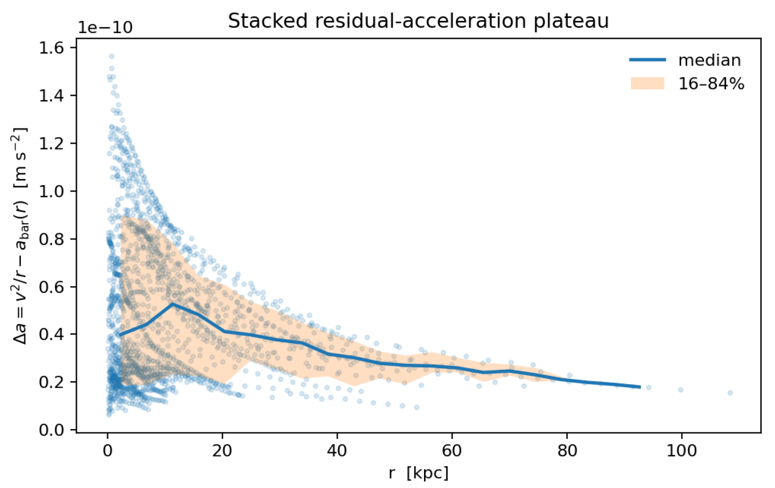
Figure 2.
Disk thickness at : joint control by geometry and surface density. Panel (a) illustrates the univariate trend, motivating the inclusion of . Panel (b) visualizes the role of (color scale), for which the two-factor model explains the data significantly better than either univariate alternative.
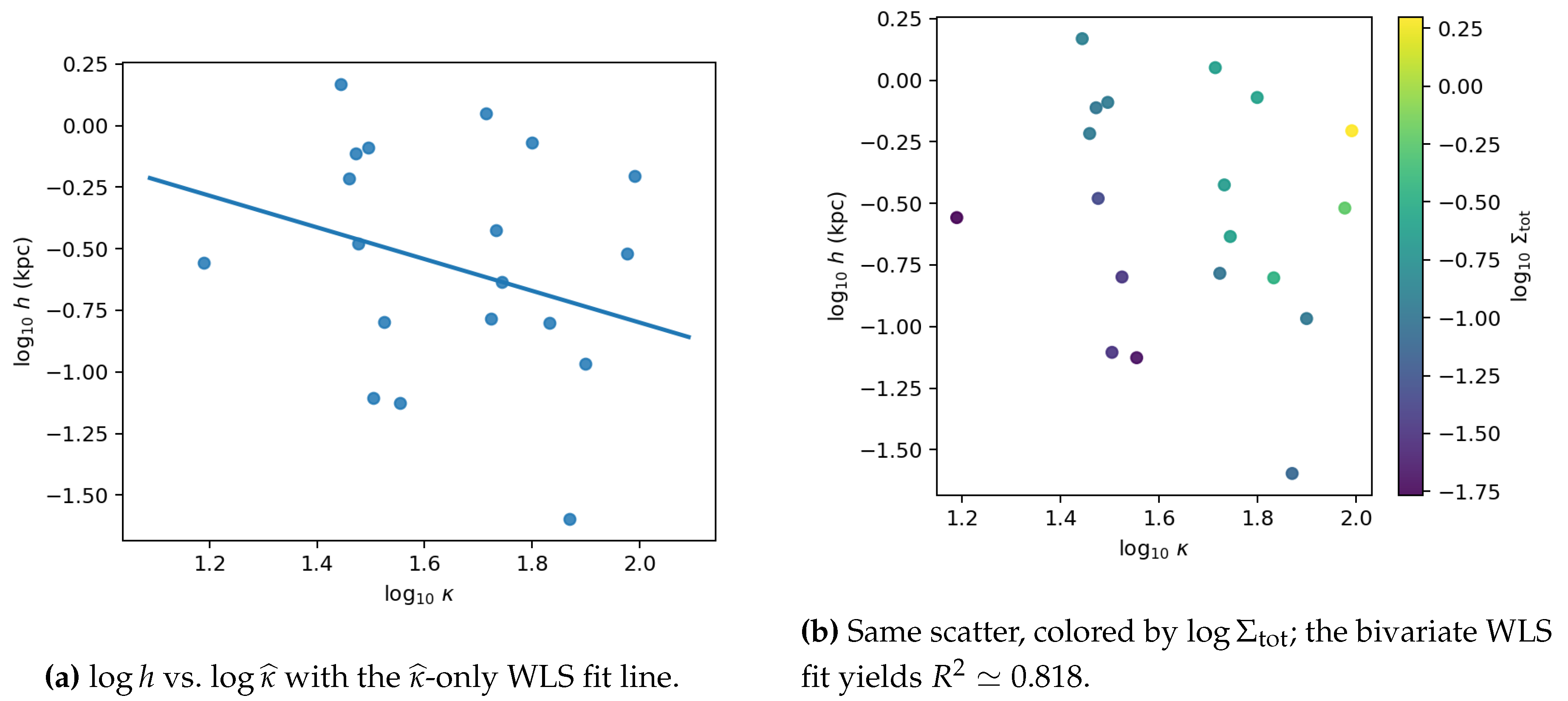
Table 1.
Parameter roles for the primary models and the diagnostic status of .
| Model | Global parameters | Per-galaxy nuisance / diagnostics |
|---|---|---|
| PTQ-screen |
(cosmology link, ) q (screening steepness; Eq. (19)) |
(baryons; Eq. (20)) (diagnostic inferred; Eq. (21)) |
| MOND | (acceleration scale) | (baryons) |
Table 2.
Effective parameter counting used for information criteria. The per-galaxy nuisance count is (one per galaxy). Global parameters are: none (baryon-only), (MOND), (PTQ-linear / PTQ-), and (PTQ-screen). Distance and inclination enter only through covariance propagation (Eq. (24)) and are not counted. The diagnostic is derived and is not counted.
| Model family | |||
|---|---|---|---|
| Baryon-only | 0 | ||
| MOND (free ) | 1 | ||
| PTQ (linear) / PTQ- | 1 | ||
| PTQ-screen | 2 |
Table 3.
Global model comparison on SPARC (Gaussian family). data points for all rows. The effective parameter count k is defined explicitly in Section 4.3 (Table 2); in particular, distance/inclination enter through covariance propagation and are not counted, and the diagnostic efficiency does not contribute to k. Model shorthand: PTQ-screen, primary model of this work; MOND (free ), standard MOND with fitted ; PTQ-, a PTQ variant using a MOND-like interpolation function; NFW-1p, a one-parameter NFW halo fit; PTQ (linear), unscreened response; Baryon-only, null model sourced solely by observed baryons.
| Model | k | N | AICfull | BICfull | AICfull | BICfull | ||
|---|---|---|---|---|---|---|---|---|
| PTQ–screen | 94 | 1782 | 1992.29 | 13772.90 | 14288.54 | 0.00 | 0.00 | |
| MOND (free ) | 93 | 1782 | 1981.71 | 13816.66 | 14326.81 | 43.75 | 38.27 | |
| PTQ– | 93 | 1782 | 2001.58 | 13817.64 | 14327.79 | 44.73 | 39.25 | |
| NFW–1p | 183 | 1782 | 3736.88 | 14656.60 | 15660.44 | 883.69 | 1371.90 | |
| PTQ (linear) | 93 | 1782 | 2039.63 | 14913.28 | 15423.43 | 1140.37 | 1134.89 | |
| Baryon-only | 92 | 1782 | 2327.24 | 19090.68 | 19595.34 | 5317.78 | 5306.80 |
Disclaimer/Publisher’s Note: The statements, opinions and data contained in all publications are solely those of the individual author(s) and contributor(s) and not of MDPI and/or the editor(s). MDPI and/or the editor(s) disclaim responsibility for any injury to people or property resulting from any ideas, methods, instructions or products referred to in the content. |
© 2026 by the authors. Licensee MDPI, Basel, Switzerland. This article is an open access article distributed under the terms and conditions of the Creative Commons Attribution (CC BY) license (http://creativecommons.org/licenses/by/4.0/).
Copyright: This open access article is published under a Creative Commons CC BY 4.0 license, which permit the free download, distribution, and reuse, provided that the author and preprint are cited in any reuse.


