
Submitted:
25 March 2025
Posted:
26 March 2025
You are already at the latest version
Abstract
Current flight procedure design primarily relies on expert experience, lacking a systematic approach to comprehensively balance safety, route simplification, and environmental impact. To address this challenge, this paper proposes a reinforcement learning-based method that leverages carefully crafted reward engineering to achieve an optimized flight procedure design, effectively considering safety, route simplicity, and environmental friendliness. To further enhance performance by tackling the low sampling efficiency in the Replay Buffer, we introduce a multi-objective sampling strategy based on the Pareto frontier, integrated with the Soft Actor-Critic (SAC) algorithm. Experimental results demonstrate that the proposed method generates executable flight procedures in the BlueSky open-source flight simulator, successfully balancing these three conflicting objectives, while achieving a 28.6% increase in convergence speed and a 4% improvement in comprehensive performance across safety, route simplification, and environmental impact compared to the baseline algorithm. This study offers an efficient and validated solution for the intelligent design of flight procedures.
Keywords:
Reinforcement learning
; Multi-objective optimization
; Flight procedure design
; Pareto frontier
; Soft Actor-Critic
; BlueSky simulator
1. Introduction
Flight procedures are defined as the systematic operational steps established for aircraft, delineating routes, altitudes, and speeds from takeoff to landing. These procedures constitute a fundamental component in safeguarding flight safety, optimizing operational efficiency, and mitigating environmental impacts. Based on the navigation methodologies employed, flight procedures are primarily classified into two distinct categories: Performance-Based Navigation (PBN) procedures and conventional navigation procedures. Conventional navigation procedures depend on terrestrial navigation aids, such as Very High Frequency Omnidirectional Range/Distance Measuring Equipment (VOR/DME). The design of flight routes under these procedures is constrained by the geographical coverage of ground-based stations, resulting in limited flexibility and challenges in accommodating the requirements of complex airspace environments. In contrast, PBN procedures leverage the integration of Global Navigation Satellite Systems (GNSS) with onboard navigation technologies to achieve precise alignment with aircraft performance capabilities. This enables the formulation of more accurate and adaptable flight paths [1,2], yielding substantial benefits in route simplification and noise pollution abatement [3]. Consequently, PBN has been established as the predominant standard for contemporary flight procedure design, as endorsed and promoted by the International Civil Aviation Organization (ICAO) [4].
In the design of Performance-Based Navigation (PBN) flight procedures, safety constitutes the primary objective. This mandates that flight procedures are engineered to effectively avoid terrain obstacles, airspace conflicts, and meteorological hazards. To ensure the safe operation of aircraft, this is accomplished through the delineation of protection areas and the application of Minimum Obstacle Clearance (MOC) standards [5]. Economic considerations focus on optimizing route lengths, minimizing redundant turns, and strategically planning climb gradients to reduce fuel consumption and operational costs [6,7]. Additionally, environmental sustainability has emerged as a vital supplementary principle in contemporary flight procedure design [8]. This involves mitigating noise pollution in residential areas through measures such as avoiding noise-sensitive zones and developing low-noise approach trajectories. Nevertheless, current methodologies for flight procedure design predominantly rely on manual processes. Designers typically employ tools such as Computer-Aided Design (CAD) in conjunction with established standards, such as ICAO Doc 8168 (PANS-OPS), and leverage engineering expertise. Although this approach ensures adherence to safety regulations, it frequently proves inadequate in sufficiently addressing considerations of convenience and environmental impact [9].
In recent years, there have been attempts to incorporate intelligent algorithms for optimization in flight procedure design; however, these efforts are still beset by significant limitations. For instance, methods based on reinforcement learning (RL) explore feasible flight paths through the interaction of an agent with the environment [10,11]. Nonetheless, most studies focus solely on a single objective, such as minimizing path length or energy consumption, failing to integrate safety, convenience, and environmental considerations into a unified reward framework. This results in an inadequate capacity for multi-objective trade-offs.Moreover, existing RL approaches lack refined designs for critical factors such as noise impact modeling and dynamic adjustment of protection areas, which restricts their practical applicability in real-world flight procedures [12]. On the other hand, multi-objective optimization algorithms, such as genetic algorithms, can generate Pareto front solutions but rely on offline computations and fixed weight assignments [13]. These methods struggle to adapt to dynamic environments and real-time decision-making requirements. Additionally, they perform poorly when handling complex constraints, such as obstacle avoidance and noise control [14].The limitations of these methods in flight procedure design underscore the urgent need for a more systematic and flexible optimization framework to address these challenges effectively [15].
The application of intelligent algorithms in aviation optimization has garnered increasing research attention; however, a notable research gap remains in effectively balancing multiple objectives within flight procedure design. The study by Gardi et al. demonstrates the potential of Pareto optimization methods to enhance safety, efficiency, and environmental performance in flight trajectory design [16].By leveraging multi-objective optimization algorithms, this approach successfully reduces fuel consumption while simultaneously improving flight efficiency. Nevertheless, its limitations arise from a reliance on predefined weight assignments and a static optimization framework, which lacks adaptability to dynamic operational environments. Consequently, it is unable to adjust design parameters in real time to address complex constraints, such as unexpected obstacles or meteorological variations. Additionally, the omission of environmental objectives, such as noise pollution, from the optimization framework results in insufficient mitigation of environmental impacts.
Similarly, Ribeiro et al. (2022) highlight the effectiveness of reinforcement learning (RL) in optimizing airspace structure under complex constraints [17]. Through dynamic adjustments to airspace configurations, this method significantly enhances airspace utilization and operational efficiency. However, the research is limited to structural adjustments and fails to address the inherent multi-objective trade-offs in flight procedure design, particularly the simultaneous optimization of safety (e.g., obstacle avoidance), efficiency (e.g., fuel consumption), and environmental impact (e.g., noise reduction). Furthermore, the reward function design in this study is relatively simplistic, inadequately capturing the conflicts and synergies among multiple objectives, which limits its practical applicability in flight procedure design.
To address the aforementioned issues, this paper introduces a reinforcement learning algorithm that quantifies safety, convenience, and environmental sustainability into a weighted reward function, combined with a dynamic weight allocation mechanism to achieve multi-objective collaborative optimization. By continuously adjusting the coordinates of the waypoints to be modified, the final trajectory design for the entire departure flight procedure is realized. The main contributions of this paper are as follows:
- A multi-objective sampling strategy based on the Pareto front is proposed to enhance algorithm efficiency. To address the low sampling efficiency associated with offline reinforcement learning algorithms, this study introduces a multi-objective sampling strategy grounded in the Pareto front, which is integrated with the Soft Actor-Critic (SAC) algorithm. Experimental results indicate that this approach improves convergence speed by 28.6% and increases the multi-objective composite score by 4%. By optimizing the exploration and exploitation of the state space, the proposed method significantly enhances algorithm efficiency, rendering it particularly suitable for the rapid convergence and computational efficiency requirements in flight procedure design.
- A reinforcement learning environment that encompasses safety, simplicity, and environmental sustainability in flight procedure design tasks is established. Within the reinforcement learning framework, this research constructs an environment for flight procedure design tasks that comprehensively considers the multi-objective optimization of safety, simplicity, and environmental sustainability. Through meticulous reward engineering, the research team identifies a suitable set of reward functions that effectively address these conflicting optimization objectives. These reward functions not only balance the trade-offs among different objectives but also guide the reinforcement learning algorithm in discovering optimal strategies for complex flight tasks.
- The executability and performance of the flight procedures are validated. The designed flight procedures are executed within the BlueSky open-source simulation platform. Experimental results demonstrate that the flight procedures developed using the proposed method are executable.
2. Related work
2.1. Flight Procedure Design
Currently, flight procedure design methodologies predominantly rely on expert experience and established guidelines, including the ICAO’s PANS-OPS (Procedures for Air Navigation Services - Operations) and the FAA’s TERPS (Terminal Procedures). These approaches emphasize compliance with safety regulations and are extensively utilized in the development of Standard Instrument Departures (SIDs) and approach procedures.For instance, the guidelines outlined in the relevant document [18] indicate adherence to ICAO Doc 8168, which is designed to ensure obstacle clearance and flight safety. However, it is noted that these methodologies often prioritize safety, potentially compromising convenience and environmental considerations.
Research indicates that traditional methods exhibit significant shortcomings in balancing safety, convenience, and environmental considerations. Firstly, while safety remains the primary objective, this focus can lead to complex procedures that increase the workload for pilots and air traffic controllers, thereby diminishing convenience. Secondly, environmental aspects, such as reducing fuel consumption and noise, are often overlooked. For instance, relevant research [19] highlights the importance of considering noise abatement procedures during the design process; however, in practice, environmental goals are frequently overshadowed by operational efficiency. Furthermore, a study by E. Israel et al. [20] suggests that while it is feasible to assess environmental impacts, the existing approach still lacks a systematic framework capable of simultaneously optimizing all objectives.
Global aviation modernization initiatives, such as the United States’ NextGen and Europe’s SESAR, emphasize efficiency and environmental sustainability. However, existing research, such as that conducted by YY Lai [21], indicates that progress in incorporating environmental considerations within flight procedure design has been limited. Specifically, it is challenging to achieve a balance among safety, convenience, and environmental sustainability in the context of multi-objective optimization. Consequently, there is an urgent need for more intelligent solutions in current methodologies.

Table 1.
Comparison of Different Methods.
| Method | Current Status | Safety | Convenience (Trajectory Shortening) | Environmental Consideration |
|---|---|---|---|---|
| CAD Tools (Traditional Design) | Rely on expert experience and standard regulations, widely used | Emphasizes safety compliance, lacks dynamic adaptability | Fixed routing, possible extended trajectory | Noise and emissions not fully considered |
| Heuristic Approach | Balances fuel and time, highly computational, already in use | Safety is treated as a constraint, not directly optimized | Subjective weight assignment, affects efficiency | Noise and fuel optimization, complex trade-off |
| Reinforcement Learning (RL) | Emerging technology, dynamic strategy adjustment, limited application | Training instability, no guaranteed safety | Potential for shortened trajectory, high data requirement | Theoretically can optimize noise and emissions |
2.2. Sampling Strategies in Reinforcement Learning
TThe sampling strategy in reinforcement learning significantly influences the learning efficiency and performance of algorithms. Traditional uniform sampling strategies, while simple and unbiased, have notable limitations. They fail to distinguish the importance of experiences, often overlooking critical turning points, which reduces sample utilization [22]. Additionally, in sparse reward scenarios, uniform sampling necessitates extensive data to cover essential areas, leading to slow convergence [23].
To address these challenges, various improved sampling strategies have been proposed. Notably, Prioritized Experience Replay (PER) has gained attention for its effectiveness [22]. PER employs a priority mechanism based on temporal-difference (TD) error, allowing for more efficient utilization of critical experiences, thus accelerating convergence. The priority of each experience is defined as (1)
where is the TD error and is a small constant to prevent zero sampling probability. Research indicates that PER can enhance sample efficiency by 3–5 times [22]. However, PER introduces bias due to non-uniform sampling, which alters the distribution of gradient updates. To mitigate this, importance sampling (IS) weights are used for bias correction, defined as (2)
where controls the correction strength. With appropriate decay of , PER can converge to the same optimal policy as uniform sampling [24].
In addition to PER, other sampling strategies have been developed. Model-based priority methods utilize a dynamics model to predict future state values, but their effectiveness relies on model accuracy [25]. Hierarchical importance sampling segments experiences by time or features, yet often depends on prior knowledge, limiting adaptability [26]. Exploration-driven sampling prioritizes samples from underexplored states, enhancing exploration efficiency but requiring careful balance to avoid policy destabilization [27].
In summary, while uniform sampling is easy to implement, it suffers from low efficiency and slow convergence [22]. PER improves sampling efficiency but introduces bias and complexity [22,24]. Future research may focus on adaptive priority mechanisms, distributed priority architectures [28], and deeper theoretical analyses of PER, aiming to enhance the performance and practicality of reinforcement learning algorithms.
3. Methodology
3.1. Problem Formulation
In this work, models are developed for optimizing aircraft departure procedures, focusing on safety through protection zones and obstacle clearance, simplicity via turn angle and path length, and environmental impact based on noise pollution.
3.1.1. Safety
Safety is the primary objective of optimization, and its assessment is based on the establishment of protected areas for each segment between waypoints. The design of these protected areas must adhere to the requirements for straight-out departures, ensuring that aircraft can avoid ground obstacles during the takeoff phase, thereby safeguarding flight safety [29].
The departure protection area is divided into a primary zone and a secondary zone.As shown in the Figure 1. The primary zone is the area directly above the aircraft’s departure trajectory, while the secondary zone extends to the sides of the primary zone, with dimensions equal to those of the primary zone. This study evaluates the safety of different departure segments by observing obstacle information within the protected areas. When obstacles are present within these areas, the aircraft may need to adjust its climb gradient to avoid them. In this process, particular attention is given to the impact of Obstacle Identification Surfaces (OIS), which serve as an important reference for identifying route obstacles [30].
According to the regulations set forth by the International Civil Aviation Organization (ICAO), the minimum climb gradient for an aircraft must not be less than 0.033 [31]. When the actual climb gradient of the aircraft exceeds this value, it indicates that the aircraft must undertake a steeper ascent to avoid obstacles, which can compromise safety. Conversely, if the aircraft can maintain a climb gradient of 0.033 within the protected area, and there are no obstacles present in both the primary and secondary zones, it signifies that the departure segment of the aircraft possesses a high level of safety.The Obstacle Identification Surface (OIS) is a distinct sloped area designed for the effective identification and assessment of obstacles within the departure protection area, as illustrated in the Figure 2.
Specifically, the safety settings are categorized into three ratings: low, medium, and high. The highest rating indicates that there are no obstacles within the protected area of the flight segment, resulting in a high safety level. The medium rating applies when obstacles are present within the protected area; however, due to factors such as the distance and height of the obstacles relative to the flight segment, the OIS surface does not intersect with any obstacles, and the aircraft’s climb gradient remains constant at 0.033. In this case, safety can be evaluated based on the projection distance of the obstacles to the flight segment. Lastly, the lowest safety rating is assigned when obstacles exist within the main protected area, resulting in an increased climb gradient for the aircraft. In this scenario, the higher the climb gradient, the lower the safety level, indicating that the configuration of the flight segment is unreasonable.
We define the safety objective function (3) as follows:
where is the threshold value for the distance between obstacles and the flight segment, distinguishing between "far" and "near."
3.1.2. Simplicity
In the design of aircraft departure procedures, conciseness is crucial for enhancing operational efficiency. By optimizing the process from takeoff to the integration into the flight route, the path length can be significantly reduced, thereby effectively decreasing fuel consumption and harmful emissions. During the design phase, careful consideration must be given to the turning angles and the total length of the route to ensure optimal flight paths and time management.
Conciseness is primarily determined by two factors: the total sum of the angles turned throughout the procedure and the overall length of the procedure. A larger total turning angle in the departure procedure not only increases the flight distance but also leads to additional fuel consumption and time delays. The longer the overall length of the procedure, the longer the aircraft remains airborne, resulting in increased fuel consumption and operational costs.
Under the premise of ensuring safety, a concise departure procedure should minimize unnecessary turns and flight distances. Specifically, when quantifying conciseness, attention should be focused on the total length of the procedure and the variation in turning angles. A longer total length and greater angle variation correspond to lower conciseness. This represents a dynamic range, and during the quantification process, the scaling factors and weights for each component need to be continuously adjusted through experimentation.
The convenience function (4) is expressed as follows:
where is the total turning angle, L is the total length of the procedure, and k is a constant. This function effectively reflects the relationship between the turning angle and the length of the procedure, and it is applicable for optimizing flight procedures.
3.1.3. Environmental
Environmental sustainability is also a critical consideration in air transportation. In this study, it is quantified simply in terms of its impact on noise pollution. The evaluation of the environmental sustainability of departure procedures is primarily based on the noise impact on surrounding residential areas, which is typically determined by the population density of these areas and the distance from the residential zones to the aircraft flight path.
Higher population density in residential areas correlates with greater noise impact, as more individuals are affected by the noise generated during aircraft takeoff and landing. When designing departure procedures, it is essential to avoid routing aircraft over densely populated regions to minimize disturbances to residents.
The closer the residential area is to the flight path, the greater the impact of noise pollution. Noise generated by aircraft during low-altitude flight directly affects residents on the ground, particularly during the takeoff phase when noise levels are typically elevated. Therefore, departure procedures should be designed to maintain maximum distance from residential areas to reduce the noise impact on residents.
The noise function (5) is defined as follows:
where represents the population density of the i-th residential area (people/km²), and denotes the distance from the i-th residential area to the flight path.
The parameters are defined as follows:
- : the horizontal distance (km) from the flight path to the residential area.
- : a coefficient used to control the influence of population density on noise calculations.
- : a parameter that determines the rate at which noise decreases with increasing distance from the flight path.
- N: the total number of residential areas affected by the flight path.
3.2. Reinforcement Learning for Flight Procedure Design
In the work presented in this paper, a modeling approach is proposed for the multi-objective flight procedure design problem, considering safety, convenience, and environmental sustainability from the perspective of reinforcement learning. The framework for the reinforcement learning-based flight procedure design is illustrated in the following Figure 3, and the reinforcement learning algorithm employed in this study is the Soft Actor-Critic (SAC) algorithm.
As illustrated in the figure, the entire framework can be divided into two parts: Training and Execution. The Training component is responsible for updating the neural network of the reinforcement learning algorithm, while the Execution component facilitates interaction with the environment to obtain learning samples.
In the Training phase, the replay buffer [32] stores experience tuples collected from the Execution phase. Here, s represents the current state information, a denotes the action output by the Soft Actor-Critic (SAC) algorithm, r is the scalar reward calculated by the reward model based on the new state information, which is used to evaluate the quality of the action, indicates the next state information after executing action a, and d is a termination signal indicating whether the episode has ended. These data support the training of the neural network through random sampling from the replay buffer, facilitating updates to the Q-value estimates of the Critic network, optimization of the policy of the Actor network, and adjustment of the parameters of the Target Critic network, thereby enabling continuous learning and improvement of the SAC algorithm.
In the Execution phase, the SAC algorithm outputs new waypoint latitude and longitude coordinates based on the state information. The environment computes the new state information of the flight procedure based on the input coordinates, which includes information related to safety, simplicity, and environmental sustainability, such as the relative position of obstacles, procedure gradient, total procedure length, and heading change. The new state information is subsequently processed by the reward model and the SAC algorithm. The reward model outputs a reward value based on the new state information to evaluate the quality of the actions produced by the algorithm, thereby supporting the selection of the next waypoint coordinates in the SAC algorithm.
In this study, a reward engineering approach was employed to determine the reward function. While keeping the hyperparameters of the Soft Actor-Critic (SAC) algorithm unchanged, improvements were made to the reward structure based on safety, economy, simplicity, and noise-related factors to enhance the performance of flight procedure design. Specifically, the safety reward was optimized by adjusting the magnitude and feature combinations for evaluation; the economy reward shifted from a total distance-based calculation to a more direct assessment of state features; the simplicity reward improved the calculation logic of turning characteristics to more accurately encourage concise paths; and the noise reward remained stable to continuously mitigate noise impacts.
3.3. Pareto-Based Multi-Objective Optimization
Pareto Optimality is a core concept in multi-objective optimization, introduced by economists and mathematicians. It describes an ideal state of resource allocation in which no objective can be improved without worsening at least one other objective. Formally, let represent one vector and represent another vector. It is required that and . The set of Pareto optimal solutions P is defined as those that cannot be improved without sacrificing at least one objective, and the set of solutions that dominate the objective space is referred to as the Pareto Front, representing the boundary of optimality for multiple objectives.
In the context of flight procedure design, it is essential to simultaneously optimize three competing objectives: safety (obstacle avoidance and climb gradient), simplicity (flight distance and turning angles), and environmental sustainability (noise pollution control). For instance, enhancing safety may require increasing flight distance or adjusting trajectory complexity, which in turn affects economic efficiency and noise distribution. These objectives exhibit nonlinear conflicts, making it challenging to achieve global optimality using traditional single-objective optimization or fixed-weight methods [33]. Based on Pareto optimality theory, this paper constructs a non-dominated solution set to identify the Pareto front in the objective space, thereby dynamically balancing the trade-offs among multiple objectives without the need for pre-defined weights. This approach provides a rigorous mathematical framework and decision-making basis for the comprehensive optimization of flight procedure design.
The schematic diagram of the Pareto model is illustrated in the Figure 4 below.
Improvements have been made to the buffer of the Soft Actor-Critic (SAC) algorithm by implementing a priority experience replay sampling method based on the Pareto optimal model [22]. The improved buffer is illustrated in the Figure 5. All experiences from the Pareto optimal model for departure procedures are received by the replay buffer. After data reception, the priority of each experience is evaluated based on its state within the context of the Pareto optimal model for departure procedures. Subsequently, sampling is conducted using priority experience replay according to the established priorities, which is utilized for loss calculation, gradient descent updates of the policy network, and policy improvement. This process is continuously repeated in an iterative manner.
This paper provides a scalar definition of priority, where a higher value indicates a greater priority. Each data sample is assigned an initial priority of 0.01 upon being stored in the buffer. This is intended to prevent the probability of sampling that data from becoming zero, thereby ensuring it is not excluded from selection. Furthermore, the reward function in this environment is designed according to a scalarized multi-objective approach, meaning that higher rewards indicate that the data is closer to the Pareto optimal frontier of this model. Consequently, the priority U should be positively correlated with the reward r. The priority U is primarily calculated based on the reward r and the different components of the subsequent state , as described by the following weighted sum formula (6):
Here, notice represents noise impact, safety denotes safety performance, and simplicity refers to operational simplicity, with and being the corresponding weights for each criterion. These weights are designed to address safety, convenience, and environmental factors differently.
The flowchart of the SAC algorithm using the aforementioned method is illustrated below:
| Algorithm 1 Improved SAC Algorithm with Priority-Based Replay Buffer Sampling |
|
4. Experimental Results
4.1. Experimental Setup
4.1.1. Environment Setting
In this study, a performance-based navigation (PBN) departure procedure for Luzhou Airport was developed to optimize the operational environment. The location, initial heading, and elevation information of Luzhou Airport are detailed in the table below (Table 2). Obstacle information is provided in Appendix Table A1, and population density information is presented in Table A2.
The flowchart illustrating the procedure information update process based on reinforcement learning algorithms is presented below (Figure 6):
Calculate the total horizontal length of the flight segments and update it. This step involves modifying the endpoint coordinates and starting point coordinates of all segments, and calculating the distance using the two-point distance formula.
The calculation of flight segment noise information is updated. In this step, N is calculated based on the noise from each group of people and their respective calculations. For each group of people, the noise is represented as the product of the number of people () and the distance to the observation point (). The total noise N is calculated as follows(7) and (8):
The calculation of flight segment protection information is updated. This step involves calculating the protection width based on the navigation performance of the route. However, the procedure sequence is identified by the SID (Standard Instrument Departure) during the calculation. The method for calculating is multiplied by 1.5, where indicates the navigation performance (Required Navigation Performance), with values of 0.3, 1.0, and so on. The distance is converted to nautical miles (nm) and then added to a constant of 3704. The calculation of is shown as follows(9):
This study involves the calculation and subsequent updating of the stage height. This process necessitates the revision of the safety height for each stage based on the preceding stage, followed by the computation of the average height. The determination of the stage height is contingent upon the presence of obstacles within the primary area. In the absence of such obstacles, the stage height is conventionally assumed to be 0.033. The safety height for this stage is computed as delineated in Equation (10).
If obstacles are present within the parallel projection of the main protection zone, the first step is to assess whether the Obstacle Identification Surface (OIS) intersects with these obstacles. In cases where the OIS does not intersect with any obstacles, the slope of the flight segment is maintained at the default value of 0.033, and the safety height at the end of the flight segment is calculated according to Equation (10). Conversely, if the OIS intersects with the obstacles, it is necessary to calculate the minimum obstacle clearance (MOC) required above the obstacle to determine the height needed to safely clear it. Following the clearance of the obstacle, the flight segment will ascend to the endpoint at a slope of 0.033. Under these circumstances, the safety height at the end of the flight segment, denoted as , is computed as outlined in Equation (11), where represents the height of the obstacle, denotes the distance from the obstacle to the endpoint of the flight segment, and the MOC calculation is provided in Equation (12).
The gradient is calculated as the difference between and divided by the segment length dis, resulting in the average gradient G.
The calculation of the flight segment is updated. This segment is not merely a trajectory of the aircraft but also encompasses the directional changes associated with the aircraft’s orientation.
When the flight segment information is updated, it necessitates a comprehensive revision of the information, including the trajectory, total errors, and distance updates.
The overall simplicity of the procedure has been updated. In this section, the procedure’s simplicity is calculated based on an algorithm related to heading. The initial heading difference is the heading of the first waypoint to be adjusted minus the turning angle of the starting waypoint. Next, calculate a ratio related to , based on a threshold of 120 degrees, and apply special handling for a 0-degree difference (by adding an additional 1 to the ratio), as shown in equation (13). Then, iterate through the remaining waypoints, calculating the heading difference for each pair of consecutive waypoints, and repeat a similar processing procedure to compute the corresponding ratio , which is then accumulated, as indicated in equation (14). Ultimately, the Simply value is the sum of and the accumulated , as expressed in equation (15).
The total noise of the departure procedure is updated by summing the noise values N of each segment. The total distance of the departure procedure is updated by summing the distances of each segment.
4.1.2. Reinforcement Learing Setting
Section1: Observation Space Observation Space for the SAC Algorithm in Reinforcement Learning.The observation space is defined as follows:
Table 3.
Meanings and value ranges of state observations
| State | Value Range | |
|---|---|---|
| Information about obstacles within the horizontal projection of the main protection zone of the previous segment before the current waypoint | 0-1 | |
| Information about obstacles within the horizontal projection of the secondary protection zone of the previous segment before the current waypoint | 0-1 | |
| Information about obstacles within the horizontal projection of the main protection zone of the next segment after the current waypoint | 0-1 | |
| Information about obstacles within the horizontal projection of the secondary protection zone of the next segment after the current waypoint | 0-1 | |
| Slope information of the previous segment before the current waypoint | 0-1 | |
| Slope information of the next segment after the current waypoint | 0-1 | |
| Noise information of the previous segment before the current waypoint | 0-1 | |
| Noise information of the next segment after the current waypoint | 0-1 | |
| Simplicity of the entire procedure | 0-1 | |
| Turning information at the current waypoint | 0-1 | |
| Turning information at the previous waypoint | 0-1 | |
| Turning information at the next waypoint | 0-1 | |
| Relative length information of the segments before and after the current waypoint | 0 (nearby) | |
| Information representing the total length of the procedure | 0-1 | |
| Information about the selected waypoint | 0, 0.33, 0.66, 1 | |
| Relative latitude coordinate information of the currently selected waypoint | 0-1 | |
| Relative longitude coordinate information of the currently selected waypoint | 0-1 | |
| Out-of-bounds flag | 0, 1 |
The system state is characterized by eighteen distinct observations, each designed to encapsulate specific attributes of the navigation environment and the current waypoint configuration. These observations are enumerated as follows:
- The first observation state is the main protection zone’s average impact on the water projection of the obstacle information before the current waypoint. If there are no obstacles, takes the value of 1; if there are obstacles, its value is equal to the minimum distance from the obstacle to the water projection minus the width of the protection zone. As shown in Equation (16), is a value within 0-1,refers to the width of the protected area:
- The second observation state is the average impact of the secondary protection zone on the water projection of the obstacle information before the current waypoint. If there are no obstacles, takes the value of 1; if there are obstacles, its value is equal to the minimum distance from the obstacle to the water projection minus half the width of the protection zone. The calculation for is also shown in Equation (16), taking values from 0-1.
- The third observation state is the horizontally projected obstacle information of the sub protected area for the previous leg of the currently changed waypoint. If there is no obstacle, the value of is set to 1, and if there is an obstacle, the value of is equal to the minimum vertical distance of the obstacle to the projection of the horizontal plane of the leg, , divided by the half width of the main protected area, with a range of 0-1, as shown by Formula (16).
- The fourth observation state is the horizontally projected obstacle information of the sub protected area for the leg after the currently changed waypoint. If there is no obstacle, is set to 1. If there is an obstacle, the calculation formula is also shown in Equation (16), with a value range of 0-1.
- The fifth observation state is the difference between the gradient G of the previous leg of the current waypoint and the standard climb gradient 0.033 multiplied by 100, an empirical formula with values ranging from 0-1 as shown in Equation (17).
- The sixth state observation is defined as the difference between the gradient G of the segment following the current waypoint and the standard climb gradient 0.033 is amplified 100 times. The calculation formula is as shown in Equation (17), with a value range of 0-1.
- The seventh state observation is equal to the noise information of the previous leg of the current waypoint, with a range of 0-1.
- The eighth state observation , is equal to the noise information of the previous leg of the current waypoint, with a range of 0-1.
- The tenth state observation , is obtained by dividing the leg heading turn angle before and after the current waypoint by 180 °, a value of 0-1.
- The eleventh state observation , is obtained by dividing the heading turn angle of the forward leg of the current waypoint by 180 ° from the previous leg, and is the value of 0-1.
- The twelfth state observation , is obtained by dividing the heading turn angle of the aft leg of the current waypoint by 180 ° to the next leg, a value of 0-1. , , are capable of characterizing three heading angle values that change following a change in the current waypoint.
- The thirteenth state observation represents the relative length of the segments before and after the current waypoint. The calculation formula is shown in Equation (19), where is the length of the segment before the current waypoint, is the length of the segment after the current waypoint, and is the straight-line distance from the current waypoint to the next waypoint.
- The fourteenth state observation is the value characterizing the total length of the procedure after the procedure update, which is the total length divided by six times the straight-line distance from the procedure’s starting point to its ending point, still an empirical formula, with values ranging from 0-1.
- The Fifteenth Status Observation is the currently selected waypoint, taking the values 0, 0.33, 0.66, 1.
- The sixteenth state observation represents the relative latitude coordinate of the currently selected waypoint, with a restricted range from N28.8059978° to N29.8059978°. If an action causes the coordinate to go out of bounds, the observation retains the same coordinate as the previous time step, and the out-of-bounds flag is set to 1.
- The seventeenth state observation represents the relative longitude coordinate of the currently selected waypoint, with a restricted range from E104.7859778° to E105.7859778°. If an action causes the coordinate to go out of bounds, the observation retains the same coordinate as the previous time step, and the out-of-bounds flag is set to 1.
- The eighteenth state observation is the out-of-bounds flag. It is set to 1 when and exceed their respective boundaries, or when . In all other cases, it indicates that there is no out-of-bounds condition and is set to 0.
Section 2: Reward Function
The design of the reward function takes into account multiple factors, including safety, angular simplicity, distance simplicity, and environmental protection. A scalarization method for multi-objective optimization is used to assign corresponding weights to each factor, balancing the priorities and impacts among different objectives. Specifically, the safety reward aims to ensure stability and risk avoidance during system operation; the angular simplicity reward is used to optimize the smoothness and simplicity of paths or actions; the distance simplicity reward focuses on reducing unnecessary movements or resource consumption; and the environmental protection reward encourages energy conservation and sustainable development. In terms of weight allocation, the importance of each factor is quantified and adjusted based on the differing demands of practical application scenarios to achieve an optimal overall performance solution. Subsequently, the reward function is further determined and optimized through reward engineering, with specific experimental design and result analysis detailed in the following reward engineering experiment chapter.
Section 3: Neural Network Parameter Settings
The learning rate is set to , which is a relatively small value that helps ensure the stability of gradient descent and avoids excessive update steps that could lead to oscillation or divergence. The discount factor of 0.98 indicates that the algorithm places more emphasis on long-term rewards, making it suitable for tasks that require long-term planning. The soft update coefficient of 0.05 controls the smooth updating of the target network; a smaller value helps reduce the difference between the target network and the online network, enhancing training stability.
The experience replay buffer size is set to 20,000, allowing for sufficient historical experience storage to support the experience replay mechanism, which breaks the temporal correlation between samples. A mini-batch size of 1024 balances computational efficiency with the accuracy of gradient estimation, making it suitable for medium-scale deep network training. The network structure indicates that both the Actor and Critic networks adopt a deep structure, with the first five layers containing 256 neurons each and the last two layers expanded to 512 neurons, enhancing the network’s ability to express complex state-action mappings. The choice of the ReLU activation function helps alleviate the vanishing gradient problem while maintaining computational efficiency.
Table 4.
Neural Network Parameter Settings
| Parameter | Value | Description |
|---|---|---|
| Learning Rate | Controls the step size of optimization, affecting convergence speed. | |
| Discount Factor | 0.98 | Indicates the importance of future rewards, affecting long-term planning. |
| Soft Update Coefficient | 0.05 | Controls the smoothness of the target network updates, enhancing training stability. |
| Experience Replay Buffer Size | 20,000 | Stores sufficient historical experiences to support the experience replay mechanism. |
| Mini-batch Size | 1024 | Balances the size of updates, improving gradient estimation accuracy. |
| Network Structure | [256, 256, 256, 256, 256, 512, 512] | Indicates the deep structure of the Actor and Critic networks. |
| Activation Function | ReLU | Helps alleviate the vanishing gradient problem, enhancing computational efficiency. |
4.1.3. Priority-Based Replay Buffer Sampling Setting
According to the formulas in the previous sections (referencing earlier equations), the score for noise is calculated as shown in Equation (20), which is derived from the sum of the values of and that represent the noise information of the previous and subsequent flight segments.
The safety score is determined by the values of and from the state after the action, which represent the obstacle information in the safe zones of the previous and subsequent flight segments. The safety score is set to 1 only when and are all equal to 1; otherwise, it is set to 0.
The simplicity score consists of two parts. represents the simplicity of the procedure; when it is greater than 0.1, ten times the value of is added to the simplicity score. The second part is determined by the total length information of the procedure represented by ; when its value is less than 0.4, twenty times the difference between 0.4 and is added to the simplicity score. Note that if any condition is not met, the score for that part is 0, and the calculation formula is given in Equation (21).
After calculating the priority U based on the above, when the algorithm needs to sample from the Replay Buffer, the sampling function computes the probability distribution of all data based on priority and samples data according to this distribution, thus achieving prioritized experience replay based on the Pareto optimal model. In this paper, and are all set to 1.
However, since the algorithm primarily learns from experiences with high rewards that lie on the Pareto front, it may lead to a larger variance in rewards when the learned policy is executed in practice. This is because the algorithm has not learned how to handle low or medium reward situations. When encountering previously unlearned low-reward states, the reward curve can fluctuate significantly.
Therefore, this paper optimizes the above issue through dynamic adjustment of the learning rate. The algorithm performs well when encountering previously learned high-reward states, but when the reward is below a certain threshold after an episode—indicating that it has encountered previously unlearned low-reward states—the learning rate of the Actor-Critic (AC) network is increased to attempt to alleviate the issue of high reward variance [34].
Increasing the learning rate means adjusting the step size of parameter updates in the optimization algorithm. The learning rate is a critical hyperparameter in deep learning and other machine learning models, determining the magnitude of model weight updates in each iteration. If the learning rate is increased, the step size of the model weight updates will be larger, allowing the model to converge more quickly to the minimum of the loss function during training. However, if the learning rate is too high, it may cause the model to oscillate around the optimal value or even fail to converge [35].
4.2. Performance Evaluation
4.2.1. Reward Engineering
In this paper, a reward engineering approach is adopted to determine the reward function. The core of the reward function is centered around G from the Problem Formulation chapter. A total of three adjustments to the reward function were made, focusing on four aspects of flight procedure design: safety, economy, simplicity, and environmental friendliness. The five reward functions and their corresponding reward function curves are set as follows.
Reward function1:
The aim is to optimize the design of the flight procedure by balancing multiple objectives of safety, economy, simplicity, and noise reduction. Its mathematical expression is(22):
1. Safety Reward ()
The safety component is defined as (23):
where represent state parameters, and indicates the state variable. to contribute positively, while and contribute negatively.
2. Economic Reward ()
The economic component is represented as (24):
where is the total length of the flight procedure, and is the distance from the starting point to the endpoint of the linear flight path.
3. Simplicity Reward ()
The simplicity component is defined as (25):
In the previous definition (15) , is clearly defined.
4. Noise Reward ()
The noise reward component is expressed as (26):
where N (27)is calculated based on the environmental model in the Problem Formulation section, ensuring that the reward function remains consistent throughout the noise reward.
Based on the reward count obtained from the reward curve, as illustrated in the Figure 7, it can be observed that the reward function exhibits a continuous variation. Furthermore, it has been trained over iterations, indicating that the configuration of the reward function is not capable of completing the task requirements.
Reward function2:
The optimization objectives of the flight procedure have been further adjusted. Compared to the first version, the design has eliminated the economic objective and focuses on three aspects: safety, simplicity, and noise control. Additionally, the safety reward has been normalized, while the normalization setting for the simplicity reward has been removed. The mathematical expression of the reward function(28) is as follows:
1. Safety Reward ()
The safety reward in the updated version is expressed as (29):
where represent positive safety factors (such as safety zone distances), and represent negative risk factors (such as proximity to obstacles). The first version of the equation is . In this version, a normalization factor of 4 has been introduced to process the safety components, allowing for a more refined evaluation of the reward based on minor variations in the parameters.
The simplicity reward is defined as (30):
The reward function curve is as follows (Figure 8), from which it can be seen that the initial stage high reward indicates that the strategy is well adapted to the environment, that the mid stage descent may be correlated with multiple objective conflicts, and that the late stage stabilization at a lower level implies that the strategy converges but does not achieve desired performance.
Reward Function 3:
The third version of the reward function represents a significant improvement and expansion over the second version, aiming to optimize the performance of the flight procedure more comprehensively while enhancing adaptability to complex environmental constraints. The second version of the reward function primarily focused on three aspects: safety, simplicity, and noise control. In this version, the simplicity reward was calculated based on the turning angle, without differentiating between angle and distance simplicity, and it lacked a clear penalty for boundary violations. The third version refines the simplicity objectives by explicitly dividing them into angle simplicity and distance simplicity, optimizing for turning angles and segment distances, which significantly enhances the specificity and interpretability of the rewards. The specific settings are as follows:
The safety reward is derived from Equation (31), where takes values between 0 and 1. The previous four states are related to flight disturbance information, with no reward values for obstacles; and represent the changes in the pitch and roll angles of the flight segment. If there are deviations in the pitch and roll angles, a penalty is applied.
The angle simplicity reward is determined by the three angles affected by the current selected flight path, denoted as . If and only if this turn angle is less than 120 degrees, is considered a straight departure procedure, thus the setting state value must be less than 0.66 to obtain the angle simplicity reward. The calculation method is given by Equation (32), and the formula for the angle simplicity reward is expressed as:
The distance simplicity reward is primarily determined by , , and . Here, when the boundary flag for is set to 1, the total value of the reward function is directly set to 0 as a maximum negative reward. When the boundary flag for is 0, the calculated value of is positive, thus the value for is calculated as twice the value of . Empirically, we aim to encourage the strategy to explore within a limited distance. If the state value , which represents the total procedure length, is less than 0.3, an additional reward based on the state value is added, as shown in Equation (34).
The environmental reward is derived from the negative reward of noise. It remains an empirical formula, calculated by dividing the total noise N updated by the procedure by 10000, as shown in Equation (35):
Thus, the classification of multi-objective optimization rewards is shown in Table 5. Note that the relative weights of the rewards depend on the environment. The weights adjusted based on experimental data in this Lu Zhou departure procedure may not be applicable to other flight procedures. The total reward function in this experimental environment is derived from the sum of the safety reward, angle efficiency reward, distance efficiency reward, and environmental noise reward. The total reward function is given by equation (36):
The reward function curve is shown below. From the figure, it can be seen that the reward function curve converges around 50,000. Observing the reward curve, it shows an overall upward trend and oscillates close to a certain peak value. The trend is positive, indicating that the model has learned a good strategy. Our algorithm and environmental adjustments can be considered complete. The model weights at 2,500,000 time steps were called for visualization, and the results are shown in Figure 10.
Priority-Based Replay Buffer Sampling
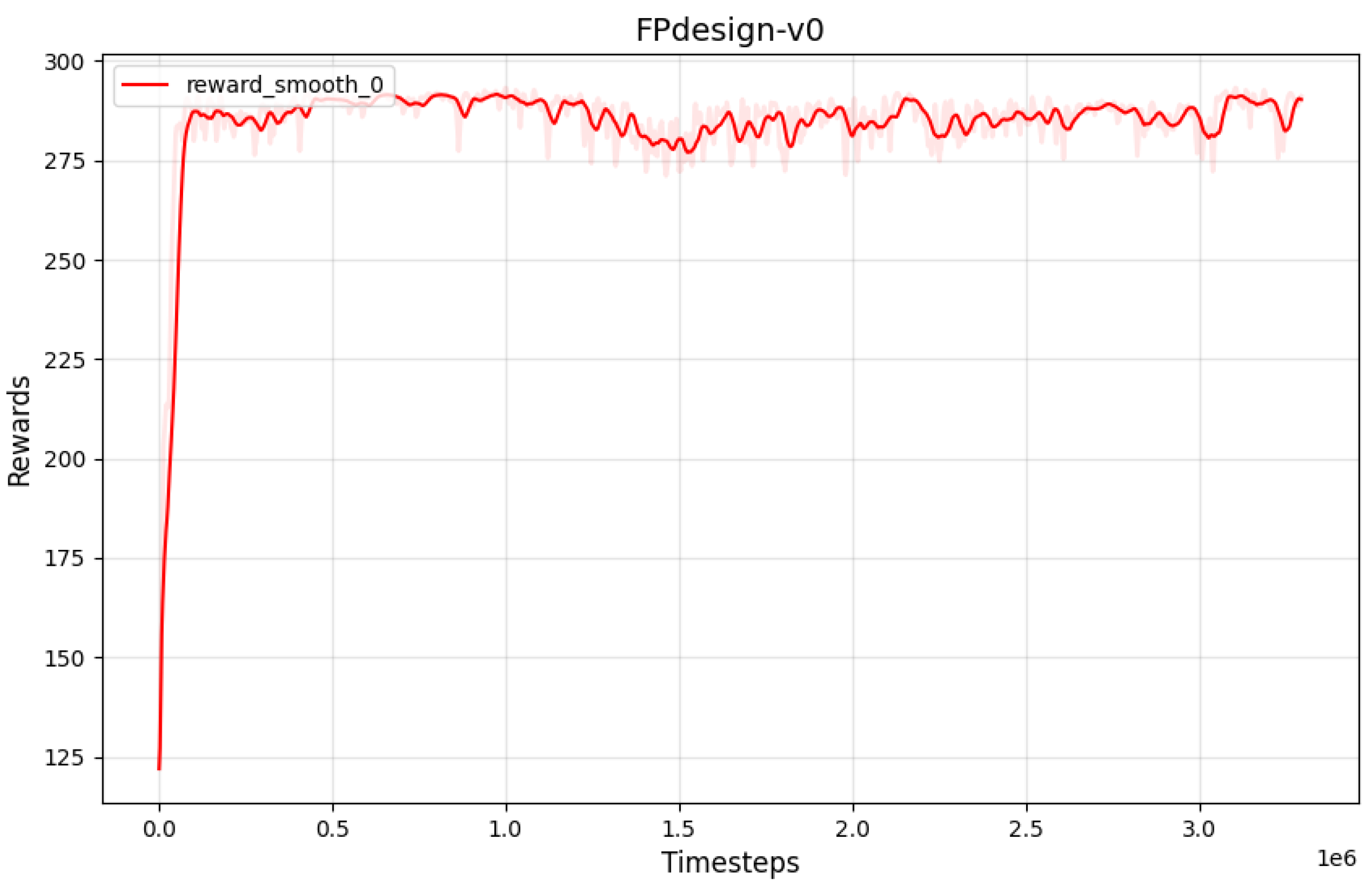
The experiment includes two comparison groups: one group applies the Soft Actor-Critic (SAC) algorithm with an unmodified sampling mechanism, while the other group employs an improved Replay Buffer and dynamic learning rate adjustment within the SAC algorithm [36]. The convergence curve of the original SAC reward is shown in Figure 9, while the reward curve of the SAC with the improved Replay Buffer and dynamic learning rate adjustment is shown in Figure 11. The reward curve of the improved SAC converges in a very short number of time steps and does not exhibit the slight decline in peak values observed in the later training stages of the original SAC algorithm. Additionally, the use of dynamic learning rate adjustment helps to keep the variance of the reward curve within a reasonable range.
Figure 9.
Original SAC Reward Curve Chart
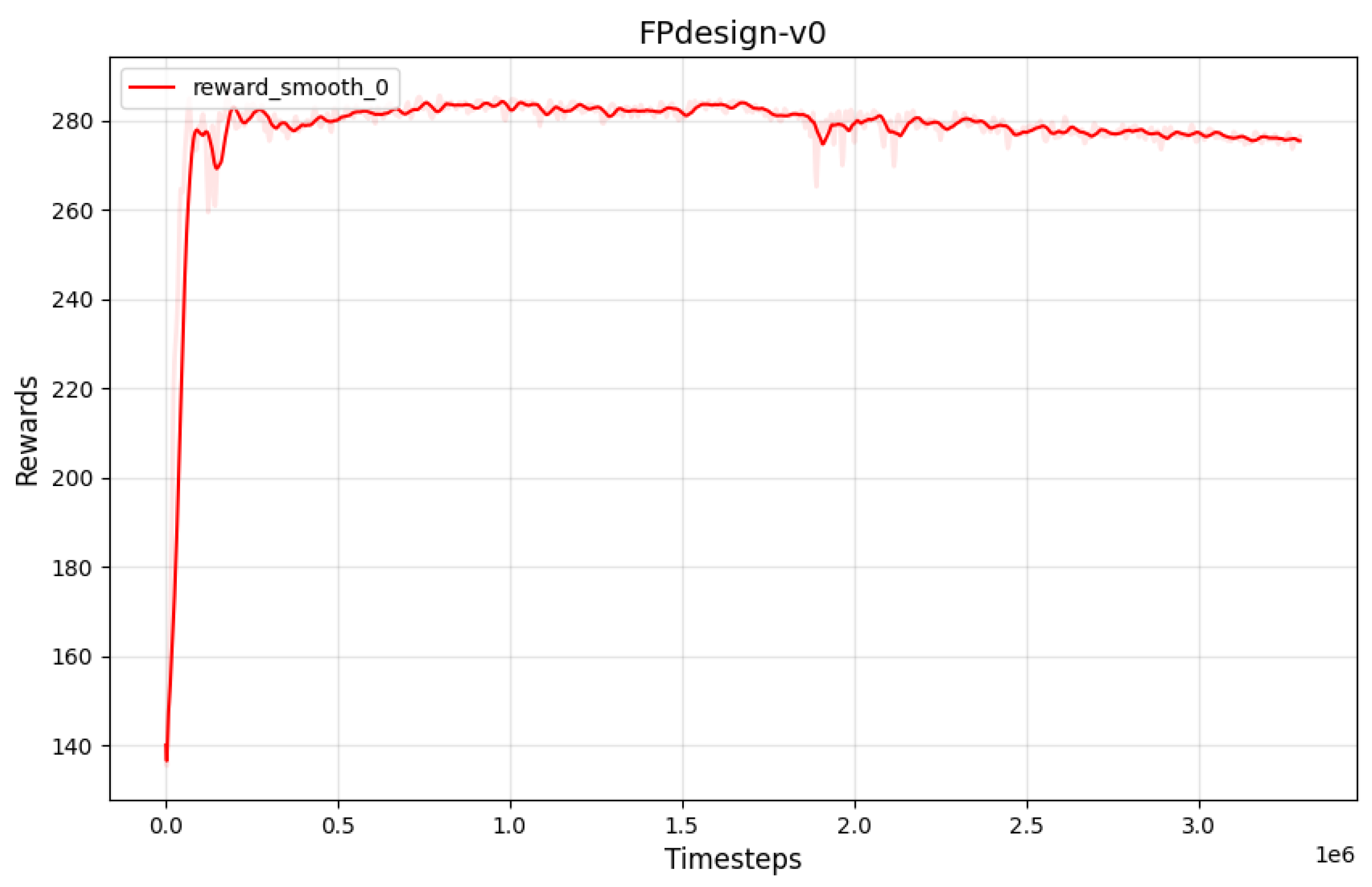
Figure 10.
procedure Visualization
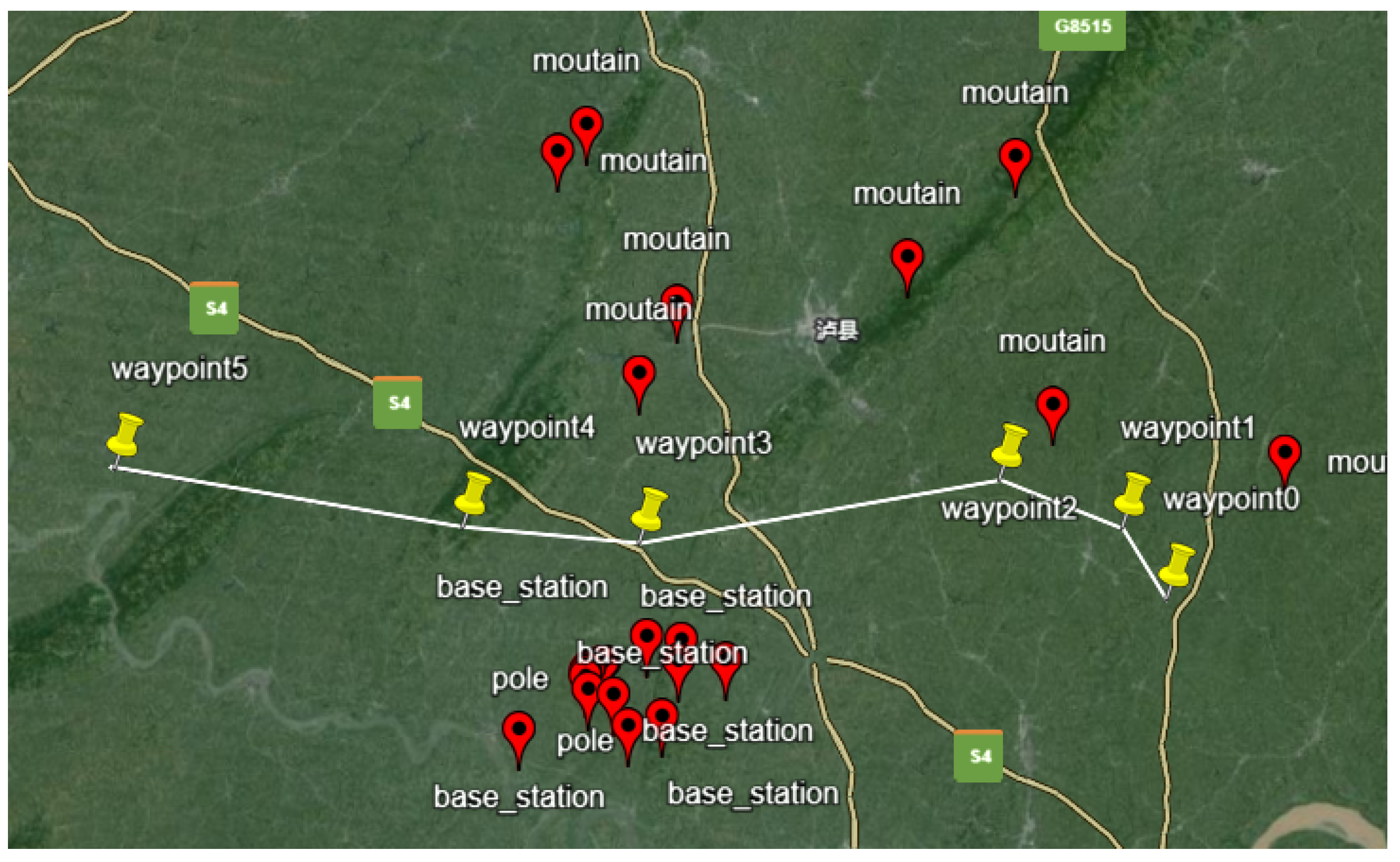
Figure 11.
Improved SAC Reward Curve Chart
By comparing the convergence curves of the reward functions for both algorithms, the results are shown in Figure 12. The analysis reveals that the convergence speeds of the two reward function curves are similar. The reward curve obtained from the improved algorithm has peak values during the convergence process that are closer to the theoretically optimal strategy. Although this method results in an increase in the variance of the reward curve, the strategy of dynamically adjusting the learning rate successfully maintains it within an acceptable range.
From the visualization results in Figure 14, it can be observed that the improved SAC algorithm demonstrates more significant effects in terms of optimization speed and results. This indicates the effectiveness of scalarization of the reward function in multi-objective optimization and proves the efficacy of the Pareto optimal prioritized experience replay sampling strategy in enhancing algorithm performance. Through experimental evaluation, the average score of the improved SAC reward demonstrates a 4% increase compared to the original SAC reward, as illustrated in the Table 6 below. Furthermore, the optimization speed of the improved method is 28.6% faster than that of the original approach. As shown in the Figure 13.
Verification of Flight Procedures Based on BlueSky
To ensure that the procedure demonstrates rationality and effectiveness under simulated real flight conditions, it is necessary to validate the flight procedure optimized by the reinforcement learning algorithm. If the procedure performs poorly in specific scenarios during the validation phase, it must be returned to the design stage for detailed adjustments until the performance of the flight procedure meets the expected standards.
This paper uses BlueSky as the validation platform for the flight procedure. BlueSky is an open-source flight simulation platform that provides a flexible and extensible environment for testing and validating various flight procedures [37].
Validating the flight procedure using BlueSky requires the creation of scenario scheme files. Next, two flight procedures optimized through multi-objective reinforcement learning are randomly selected, as shown in Figure 15 and Figure 16.
Figure 17 shows the comparison for Verification procedure 1, while Figure 18 shows the comparison for Verification procedure 2. Since the initial phase of departure is the most critical and has the lowest overlap with the simulation trajectory, this section has been enlarged for observation. By analyzing the simulated flight trajectory in conjunction with the predefined procedure trajectory, the reasonableness of the trajectory settings, protected area settings, and climb gradient is assessed based on safety, simplicity, and environmental considerations, indicating that the designed flight procedure is feasible [38].
5. Conclusions and Future Work
5.1. Conclusions
This study presents a novel reinforcement learning (RL) framework for intelligent flight procedure design, integrating multi-objective optimization to simultaneously address safety, simplicity, and environmental sustainability. By leveraging the Soft Actor-Critic (SAC) algorithm enhanced with a Pareto-based prioritized experience replay sampling strategy, we successfully trained an intelligent agent capable of autonomously optimizing Performance-Based Navigation (PBN) departure procedures. The proposed approach was validated through the design and optimization of a departure procedure for Luzhou Airport, demonstrating its feasibility and effectiveness via the BlueSky open-source flight simulation platform. Experimental results indicate that the optimized procedures effectively balance the conflicting objectives of safety (e.g., obstacle avoidance), simplicity (e.g., reduced path length and turning angles), and environmental impact (e.g., noise reduction). Compared to the baseline SAC algorithm, the improved method achieves a 28.6% increase in convergence speed and a 4% enhancement in overall performance across the multi-objective metrics, underscoring the efficacy of the Pareto-optimal sampling strategy and dynamic learning rate adjustments.
The primary innovation of this work lies in the integration of RL with Pareto-based multi-objective optimization, addressing the limitations of traditional flight procedure design methods that rely heavily on expert experience and static guidelines. Through meticulous reward engineering, we developed a comprehensive reward function that quantifies and balances safety, simplicity, and noise impact, guiding the agent toward optimal solutions. The use of a multi-objective sampling strategy further enhances sampling efficiency, overcoming the limitations of uniform sampling in conventional RL approaches. The successful execution of the optimized procedures in BlueSky confirms their practical applicability, offering a systematic and intelligent alternative to manual design processes. This study provides a robust foundation for advancing the automation and optimization of flight procedure design, with potential implications for improving airspace efficiency and sustainability in modern aviation.
Despite these advancements, several limitations remain. The validation of procedure rationality is primarily based on simulated flight trajectories, focusing on safety, simplicity, and environmental impact, without fully exploring additional factors such as pilot workload or air traffic control constraints. Furthermore, the reliance on BlueSky’s simplified kinematic models limits the fidelity of real-world force dynamics, necessitating further validation with more advanced simulators. The algorithm’s optimization is currently tailored to PBN departure procedures, with its applicability to approach or missed approach procedures yet to be established due to differing environmental complexities. Lastly, the improvements to the RL algorithm, particularly the dynamic learning rate adjustment, may not fully mitigate reward variance in all scenarios, indicating a need for deeper refinement.
5.2. Future Work
Building on the findings and limitations of this study, several avenues for future research are proposed to enhance the proposed framework and its practical utility:
Enhanced Validation with Realistic Simulators: Future work should incorporate high-fidelity flight simulators that account for real-world aerodynamic forces and operational constraints, thereby improving the credibility and robustness of validation results beyond the capabilities of BlueSky. Refinement of Algorithmic Improvements: The Pareto-optimal prioritized experience replay strategy, while effective, increases reward variance in certain scenarios. Although dynamic learning rate adjustments mitigate this issue, alternative approaches—such as adaptive priority mechanisms or hybrid sampling strategies—could be explored to achieve more stable and optimal performance. Generalization to Other Flight Procedures: The current framework is tailored to PBN departure procedures. Extending the multi-objective optimization environment and RL algorithm to accommodate approach and missed approach procedures would broaden its applicability, leveraging the experience gained from this study to create a more versatile design tool. Comprehensive Multi-Objective Modeling: The present modeling of departure procedures may not encompass all relevant factors (e.g., weather variations, airspace capacity) or be fully adaptable to other procedure types. Future efforts should aim to develop a more holistic optimization framework, potentially culminating in an autonomous flight procedure design system capable of replacing human designers. In summary, this research marks a significant step toward intelligent flight procedure design by demonstrating the potential of RL and multi-objective optimization. Addressing the identified shortcomings through these future directions will further advance the field, paving the way for fully autonomous and sustainable aviation solutions.
Appendix A. Obstacle Information at Luzhou Airport
The following table lists the obstacles around Luzhou Airport.
Table A1.
Obstacle Information.
| Obstacle Name | Position | Height (m) |
|---|---|---|
| base_station | (29.0342, 105.2909) | 361.5 |
| base_station | (29.0323, 105.3057) | 401.8 |
| High_voltage_iron_tower | (29.0245, 105.3040) | 385.6 |
| base_station | (29.0242, 105.3245) | 443.2 |
| base_station | (29.0039, 105.2957) | 428.1 |
| base_station | (29.0009, 105.2810) | 391.4 |
| Tower | (29.0128, 105.2753) | 372.6 |
| base_station | (29.0013, 105.2339) | 413.5 |
| mountain | (29.0152, 105.2645) | 364.4 |
| mountain | (29.0201, 105.2636) | 383.6 |
| pole | (29.0214, 105.2636) | 394.7 |
| mountain | (29.0224, 105.2642) | 408.9 |
| pole | (29.0227, 105.2650) | 412.6 |
| mountain | (29.0236, 105.2656) | 423.5 |
| base_station | (29.0249, 105.2713) | 467.2 |
| base_station | (29.0251, 105.2722) | 474.2 |
| mountain | (29.2315, 105.2755) | 686 |
| mountain | (29.1344, 105.2932) | 701 |
| mountain | (29.1609, 105.3113) | 732 |
| mountain | (29.1748, 105.4132) | 768 |
| mountain | (29.2119, 105.4631) | 683 |
| mountain | (29.1157, 105.4727) | 678 |
| mountain | (29.0936, 105.5725) | 695 |
| mountain | (28.4847, 105.4702) | 719 |
| mountain | (28.4245, 105.4600) | 739 |
| base_station | (28.3944, 105.3948) | 826 |
| mountain | (28.4059, 105.3858) | 883 |
| mountain | (28.3807, 105.3801) | 846 |
| mountain | (28.4230, 105.3507) | 829 |
| mountain | (28.3601, 105.3308) | 837 |
| mountain | (28.3455, 105.2859) | 851 |
| mountain | (28.4930, 105.1815) | 648 |
| mountain | (29.2213, 105.2622) | 666 |
Appendix B. Population Concentration Areas Around Luzhou Airport
The following table lists the population concentration areas around Luzhou Airport.
Table A2.
Population Concentration Areas.
| Name | Position | Number |
|---|---|---|
| yunlongzhen | (29.057965, 105.486752) | 1000 |
| deshenzhen | (29.090460, 105.413246) | 1000 |
| qifengzhen | (29.131086, 105.521877) | 800 |
| zhaoyazhen | (28.989800, 105.577030) | 1200 |
| shidongzhen | (28.992571, 105.450110) | 2000 |
| shunhexiang | (29.150573, 105.445965) | 800 |
| shaungjiazhen | (29.025615, 105.432499) | 1000 |
| luxain | (29.150530, 105.359453) | 10000 |
| niutanzhen | (29.081750, 105.338461) | 1000 |
| hushizhen | (28.948659, 105.361273) | 1000 |
| tianxingzhen | (29.105969, 105.287247) | 800 |
| haichaozhen | (28.973991, 105.281161) | 500 |
| gufuzhen | (29.140192, 105.228960) | 500 |
| huaidezhen | (29.004919, 105.222413) | 800 |
| xuanshizhen | (29.004919, 105.222413) | 1000 |
| zhaohuazhen | (29.025124, 105.118508) | 1000 |
| yinanzhen | (28.914062, 105.143877) | 800 |
| pipazhen | (29.098428, 105.071649) | 800 |
References
- Pamplona, D.A.; de Barros, A.G.; Alves, C.J. Performance-based navigation flight path analysis using fast-time simulation. Energies 2021, 14, 7800.
- Salgueiro, S.; Hansman, R.J. Potential Safety Benefits of RNP Approach Procedures. In Proceedings of the 17th AIAA Aviation Technology, Integration, and Operations Conference, 2017, p. 3597.
- Muller, D.; Uday, P.; Marais, K. Evaluation of the potential environmental benefits of RNAV/RNP arrival procedures. In Proceedings of the 11th AIAA Aviation Technology, Integration, and Operations (ATIO) Conference, including the AIAA Balloon Systems Conference and 19th AIAA Lighter-Than, 2011, p. 6932.
- López-Lago, M.; Serna, J.; Casado, R.; Bermúdez, A. Present and future of air navigation: PBN operations and supporting technologies. International Journal of Aeronautical and Space Sciences 2020, 21, 451–468.
- Tian, Y.; Wan, L.; Chen, C.h.; Yang, Y. Safety assessment method of performance-based navigation airspace planning. Journal of traffic and transportation engineering (English edition) 2015, 2, 338–345.
- Zhu, L.; Wang, J.; Wang, Y.; Ji, Y.; Ren, J. DRL-RNP: Deep reinforcement learning-based optimized RNP flight procedure execution. Sensors 2022, 22, 6475.
- Misra, S. Simulation analysis of the effects of performance-based navigation on fuel and block time efficiency. International Journal of Aviation, Aeronautics, and Aerospace 2020, 7, 7.
- Otero, E.; Tengzelius, U.; Moberg, B. Flight Procedure Analysis for a Combined Environmental Impact Reduction: An Optimal Trade-Off Strategy. Aerospace 2022, 9, 683.
- Guo, D.; Huang, D. PBN operation advantage analysis over conventional navigation. Aerospace Systems 2021, pp. 1–9.
- Zu, W.; Yang, H.; Liu, R.; Ji, Y. A multi-dimensional goal aircraft guidance approach based on reinforcement learning with a reward shaping algorithm. Sensors 2021, 21, 5643.
- Razzaghi, P.; Tabrizian, A.; Guo, W.; Chen, S.; Taye, A.; Thompson, E.; Bregeon, A.; Baheri, A.; Wei, P. A survey on reinforcement learning in aviation applications. Engineering Applications of Artificial Intelligence 2024, 136, 108911.
- Quadt, T.; Lindelauf, R.; Voskuijl, M.; Monsuur, H.; Čule, B. Dealing with Multiple Optimization Objectives for UAV Path Planning in Hostile Environments: A Literature Review. Drones (2504-446X) 2024, 8.
- Yang, F.; Huang, H.; Shi, W.; Ma, Y.; Feng, Y.; Cheng, G.; Liu, Z. PMDRL: Pareto-front-based multi-objective deep reinforcement learning. Journal of Ambient Intelligence and Humanized Computing 2023, 14, 12663–12672.
- Zhang, Y.; Zhao, W.; Wang, J.; Yuan, Y. Recent progress, challenges and future prospects of applied deep reinforcement learning: A practical perspective in path planning. Neurocomputing 2024, 608, 128423.
- Xia, Q.; Ye, Z.; Zhang, Z.; Lu, T. Multi-objective optimization of aircraft landing within predetermined time window. SN Applied Sciences 2022, 4, 198.
- Gardi, A.; Sabatini, R.; Ramasamy, S. Multi-objective optimisation of aircraft flight trajectories in the ATM and avionics context. Progress in Aerospace Sciences 2016, 83, 1–36.
- Ribeiro, M.; Ellerbroek, J.; Hoekstra, J. Using reinforcement learning to improve airspace structuring in an urban environment. Aerospace 2022, 9, 420.
- To70. Flight Procedure Design, n.d. Accessed: 2025-03-17.
- SKYbrary. Airspace and Procedure Design, n.d. Accessed: 2025-03-17.
- Israel, E.; Barnes, W.J.; Smith, L. Automating the design of instrument flight procedures. In Proceedings of the 2020 Integrated Communications Navigation and Surveillance Conference (ICNS). IEEE, 2020, pp. 3D2–1.
- Lai, Y.Y.; Christley, E.; Kulanovic, A.; Teng, C.C.; Björklund, A.; Nordensvärd, J.; Karakaya, E.; Urban, F. Analysing the opportunities and challenges for mitigating the climate impact of aviation: A narrative review. Renewable and Sustainable Energy Reviews 2022, 156, 111972.
- Schaul, T.; Quan, J.; Antonoglou, I.; Silver, D. Prioritized experience replay. arXiv preprint arXiv:1511.05952 2015.
- Hessel, M.; Modayil, J.; Van Hasselt, H.; Schaul, T.; Ostrovski, G.; Dabney, W.; Horgan, D.; Piot, B.; Azar, M.; Silver, D. Rainbow: Combining Improvements in Deep Reinforcement Learning. In Proceedings of the Proceedings of the AAAI Conference on Artificial Intelligence, 2018, Vol. 32.
- Zhang, S.; Sutton, R.S. A deeper look at experience replay. arXiv preprint arXiv:1712.01275 2017.
- Clavera, I.; Rothfuss, J.; Schulman, J.; Fujita, Y.; Asfour, T.; Abbeel, P. Model-based reinforcement learning via meta-policy optimization. In Proceedings of the Conference on Robot Learning. PMLR, 2018, pp. 617–629.
- Yin, H.; Pan, S. Knowledge transfer for deep reinforcement learning with hierarchical experience replay. In Proceedings of the Proceedings of the AAAI Conference on Artificial Intelligence, 2017, Vol. 31.
- Pathak, D.; Agrawal, P.; Efros, A.A.; Darrell, T. Curiosity-driven exploration by self-supervised prediction. In Proceedings of the International conference on machine learning. PMLR, 2017, pp. 2778–2787.
- Kapturowski, S.; Ostrovski, G.; Dabney, W.; Quan, J.; Munos, R. Recurrent Experience Replay in Distributed Reinforcement Learning. In Proceedings of the International Conference on Learning Representations, 2019.
- Yang, J.; Sun, Y.; Chen, H. Differences Between Traditional Navigation and PBN Departure Procedures and Automation of Protected Area Drawing Using AutoLISP. Modern Computer 2015, pp. 56–59.
- Dai, F. Flight Procedure Design; Tsinghua University Press and Beijing Jiaotong University Press: Beijing, 2017.
- Abeyratne, R.; Abeyratne, R. Article 38 Departures from International Standards and Procedures. In Proceedings of the Convention on International Civil Aviation: A Commentary. Springer, 2014, pp. 417–464.
- Dao, G.; Lee, M. Relevant experiences in replay buffer. In Proceedings of the 2019 IEEE symposium series on computational intelligence (SSCI). IEEE, 2019, pp. 94–101.
- Lampariello, L.; Sagratella, S.; Sasso, V.G.; Shikhman, V. Scalarization via utility functions in multi-objective optimization. arXiv preprint arXiv:2401.13831 2024.
- Yuping, H.; Weixuan, L.; Zuhuan, X. Comparative analysis of deep learning framework based on TensorFlow and PyTorch [J]. Modern Information Technology 2020, 4, 80–82.
- Goodfellow, I.; Bengio, Y.; Courville, A.; Bengio, Y. Deep learning; Vol. 1, MIT press Cambridge, 2016.
- Liu, J.; Liu, Y.; Luo, X. Research Progress in Deep Learning. Application Research of Computers 2014, 31.
- Hoekstra, J.M.; Ellerbroek, J. Bluesky ATC simulator project: an open data and open source approach. In Proceedings of the Proceedings of the 7th international conference on research in air transportation. FAA/Eurocontrol Washington, DC, USA, 2016, Vol. 131, p. 132.
- Federal Aviation Administration. Instrument Flight Procedure Validation (IFPV) of Performance Based Navigation (PBN) Instrument Flight Procedures (IFP), 2023.
Figure 1.
Straight-Out Departure Protected Area.
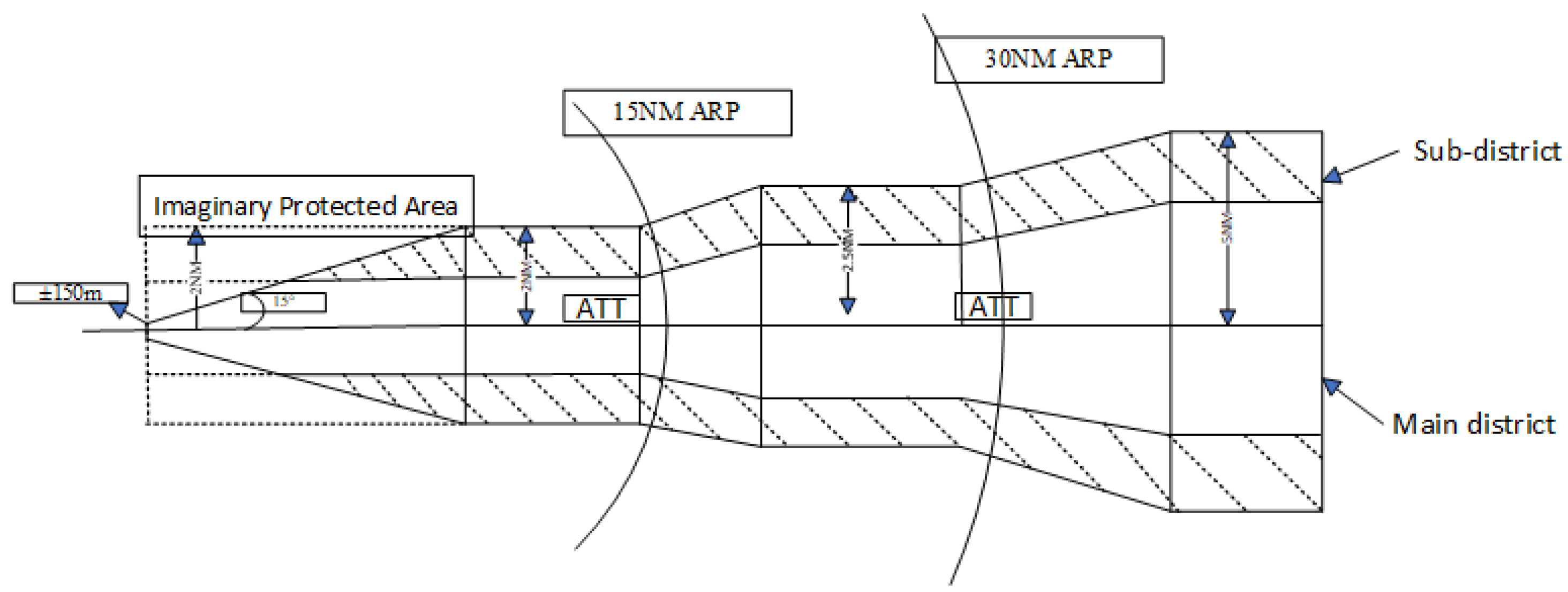
Figure 2.
Obstacle Identification Surface.
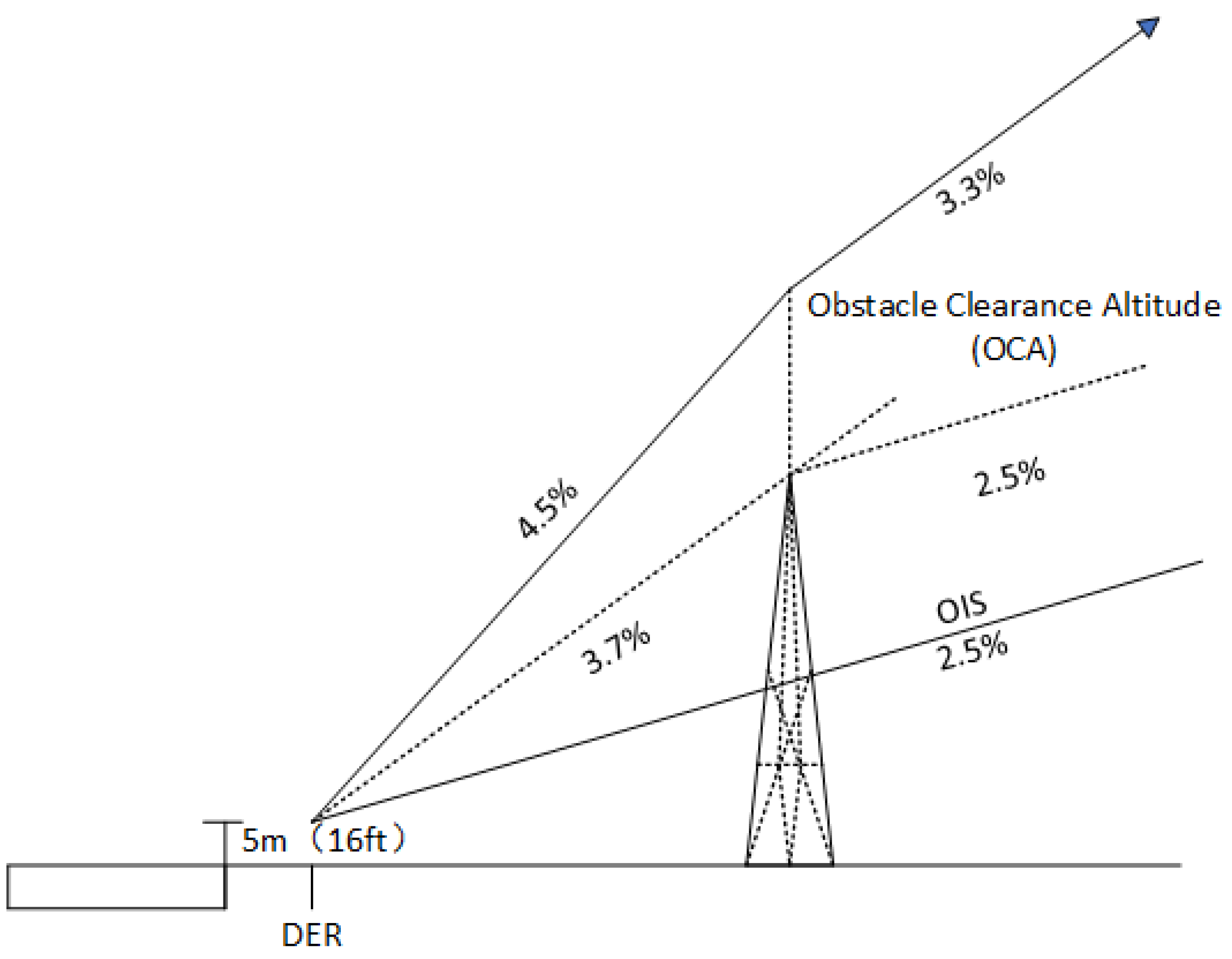
Figure 3.
Framework for Reinforcement Learning-Based Flight Procedure Design.
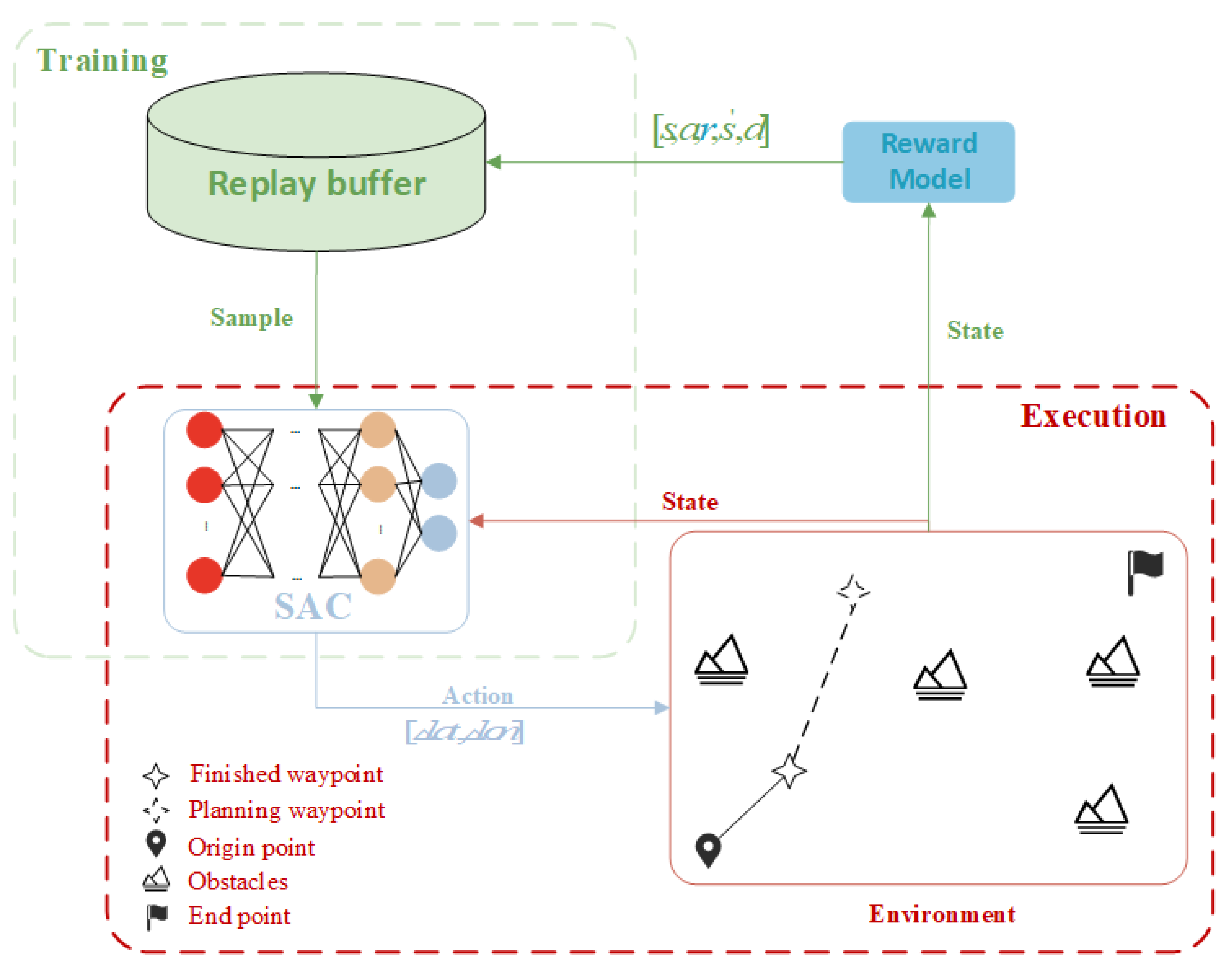
Figure 4.
Schematic Diagram of the Pareto Model for Departure Procedures.
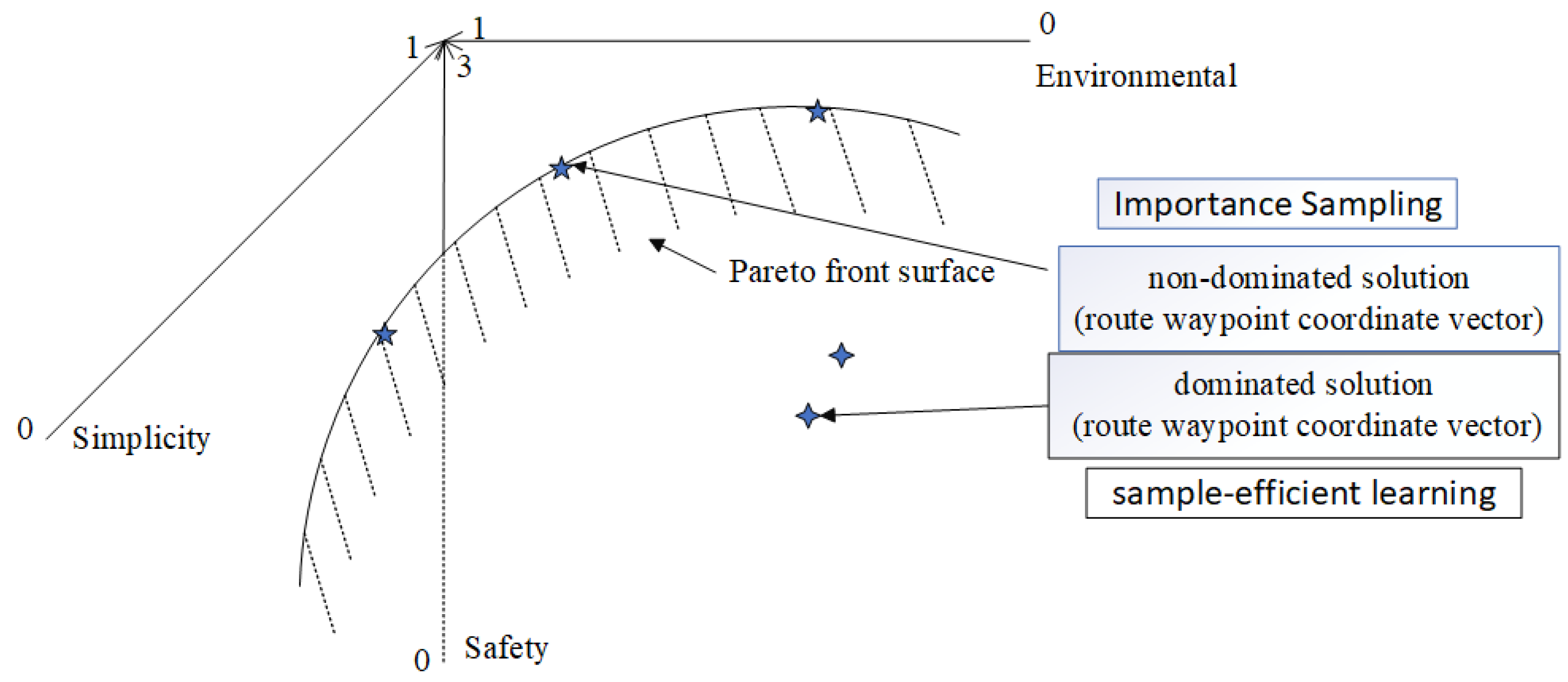
Figure 5.
Schematic Diagram of the Replay Buffer Structure.
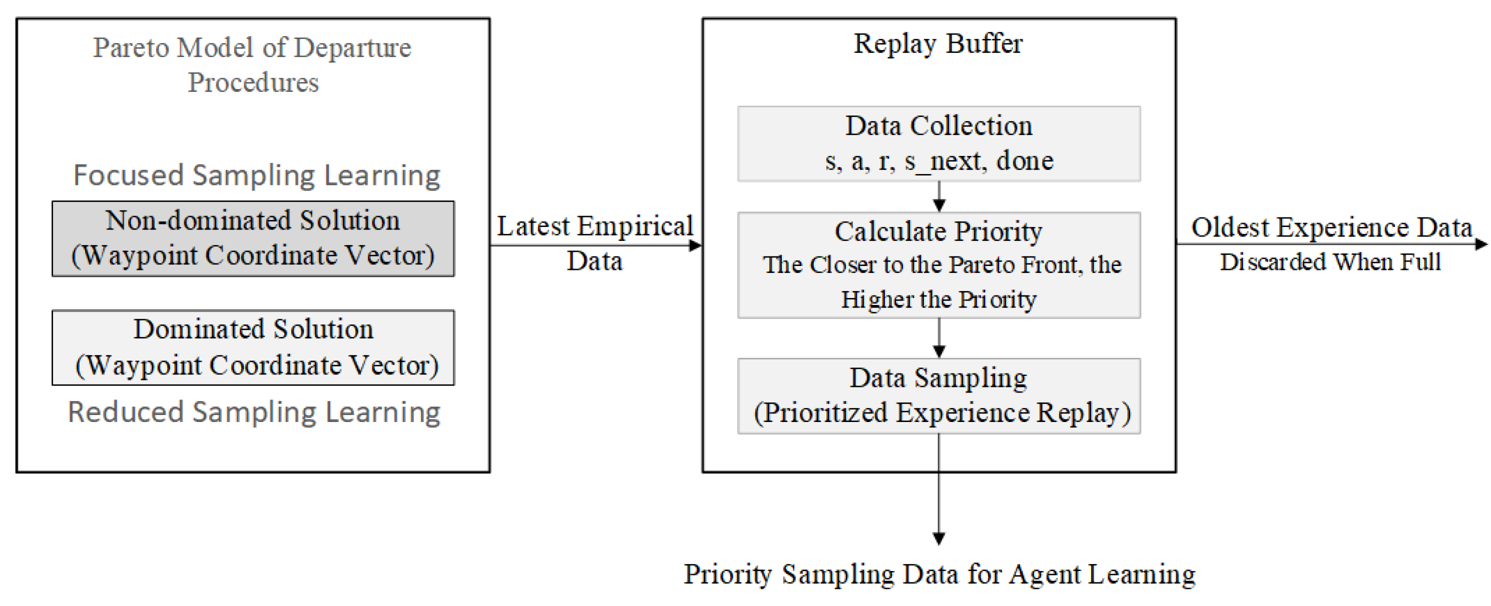
Figure 6.
Flowchart of the procedure Update Process.
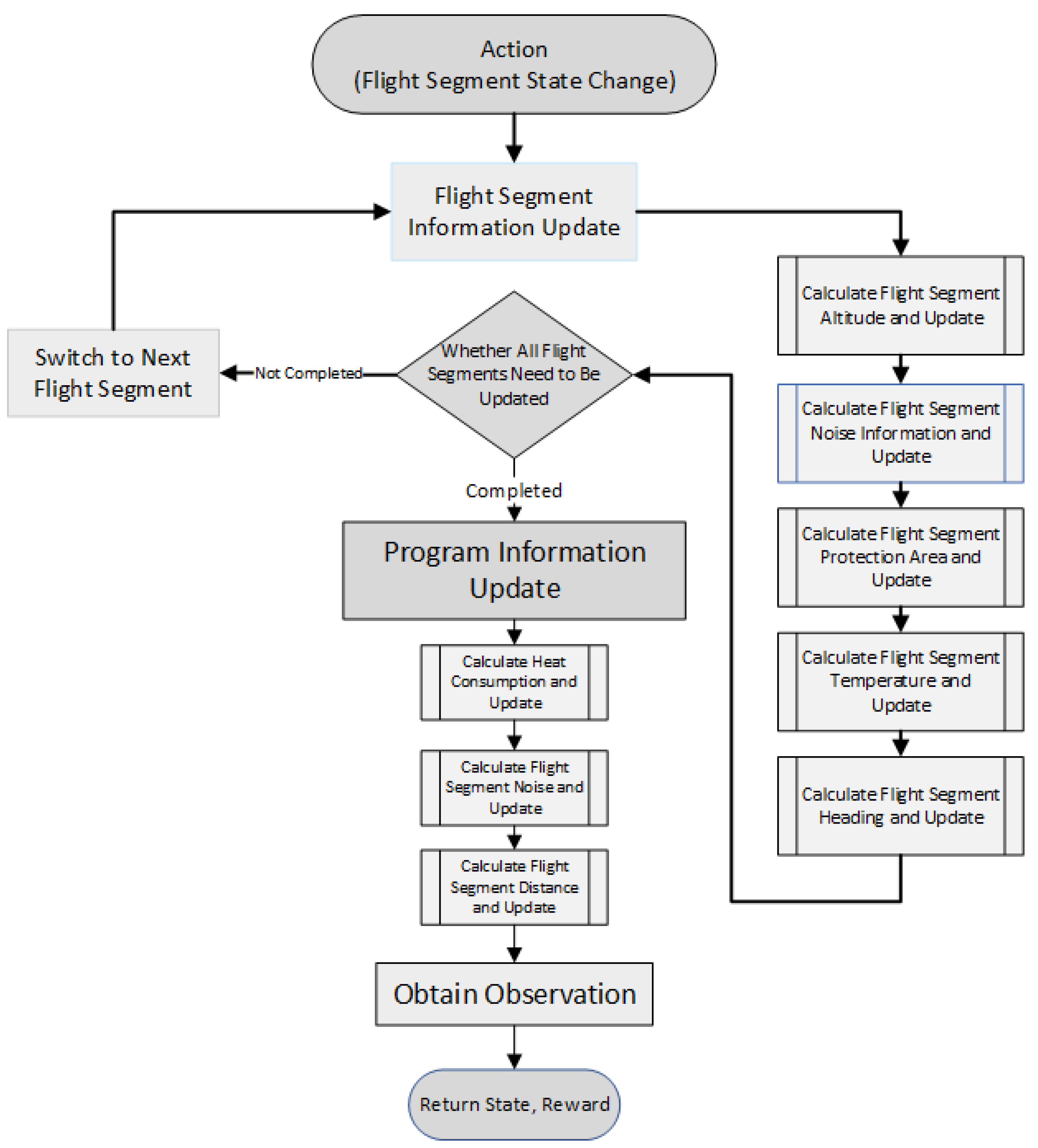
Figure 7.
Illustration of the Reward Curve-v0
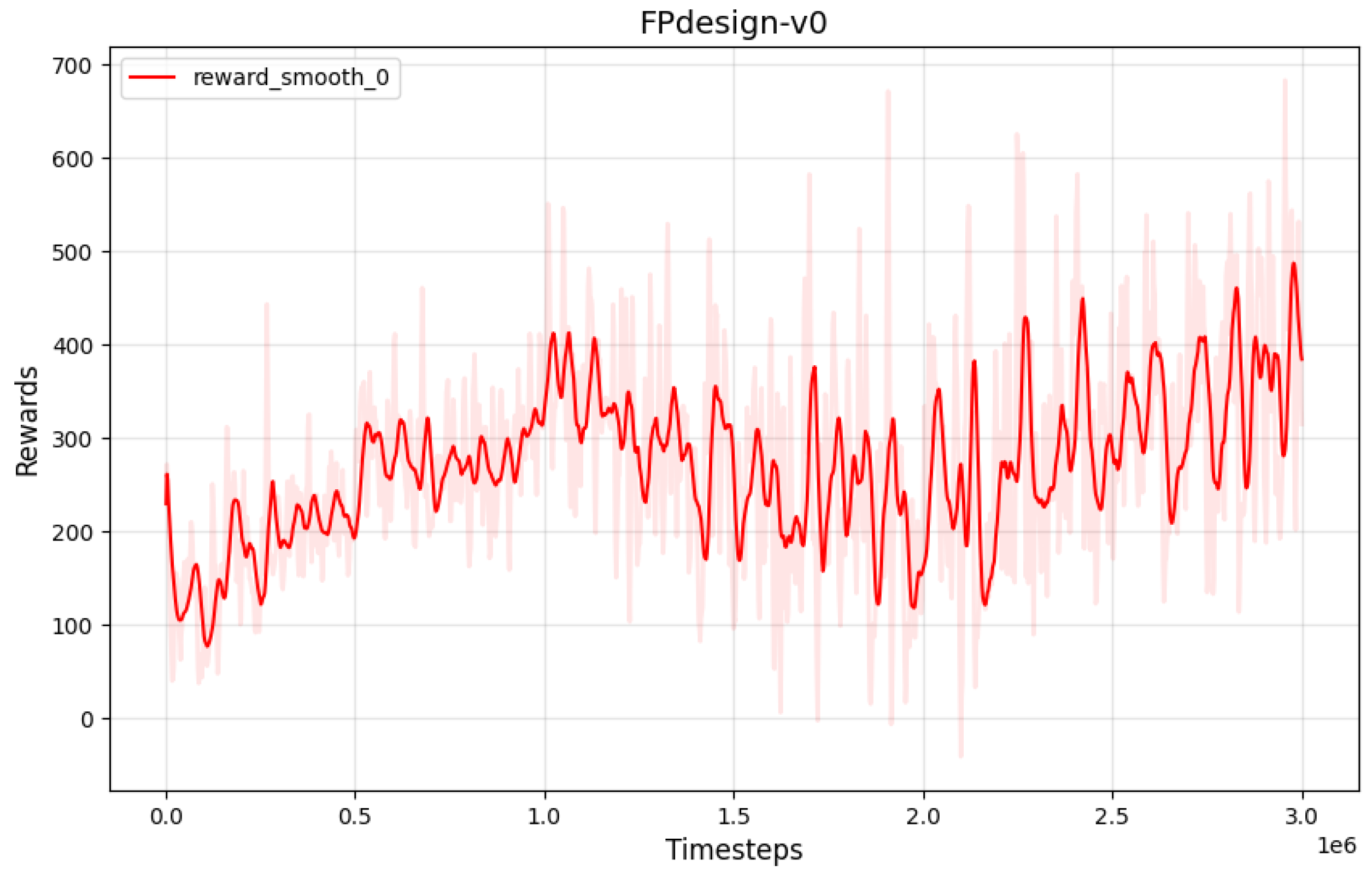
Figure 8.
Illustration of the Reward Curve-v1
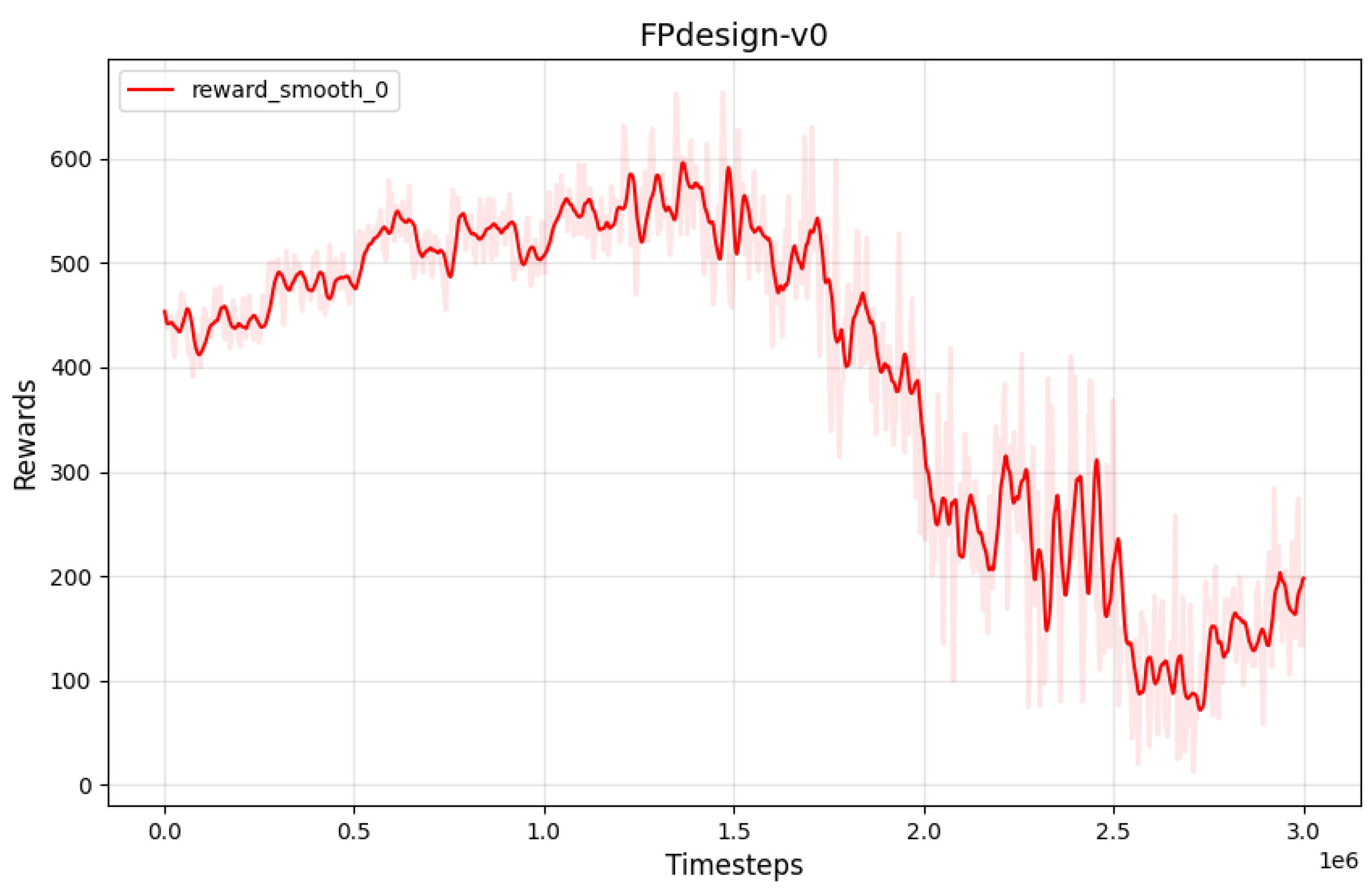
Figure 12.
Reward Curve Comparison Chart
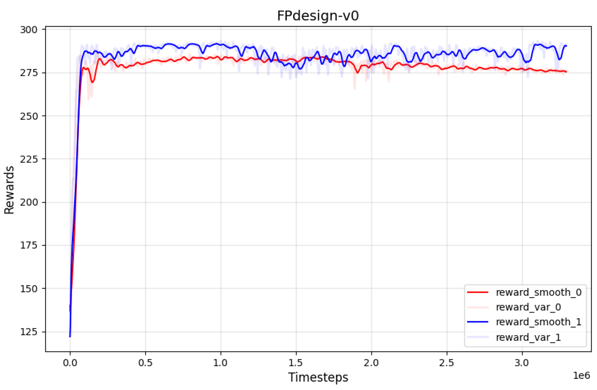
Figure 13.
Comparison of Convergence Speed Before and After Improvement
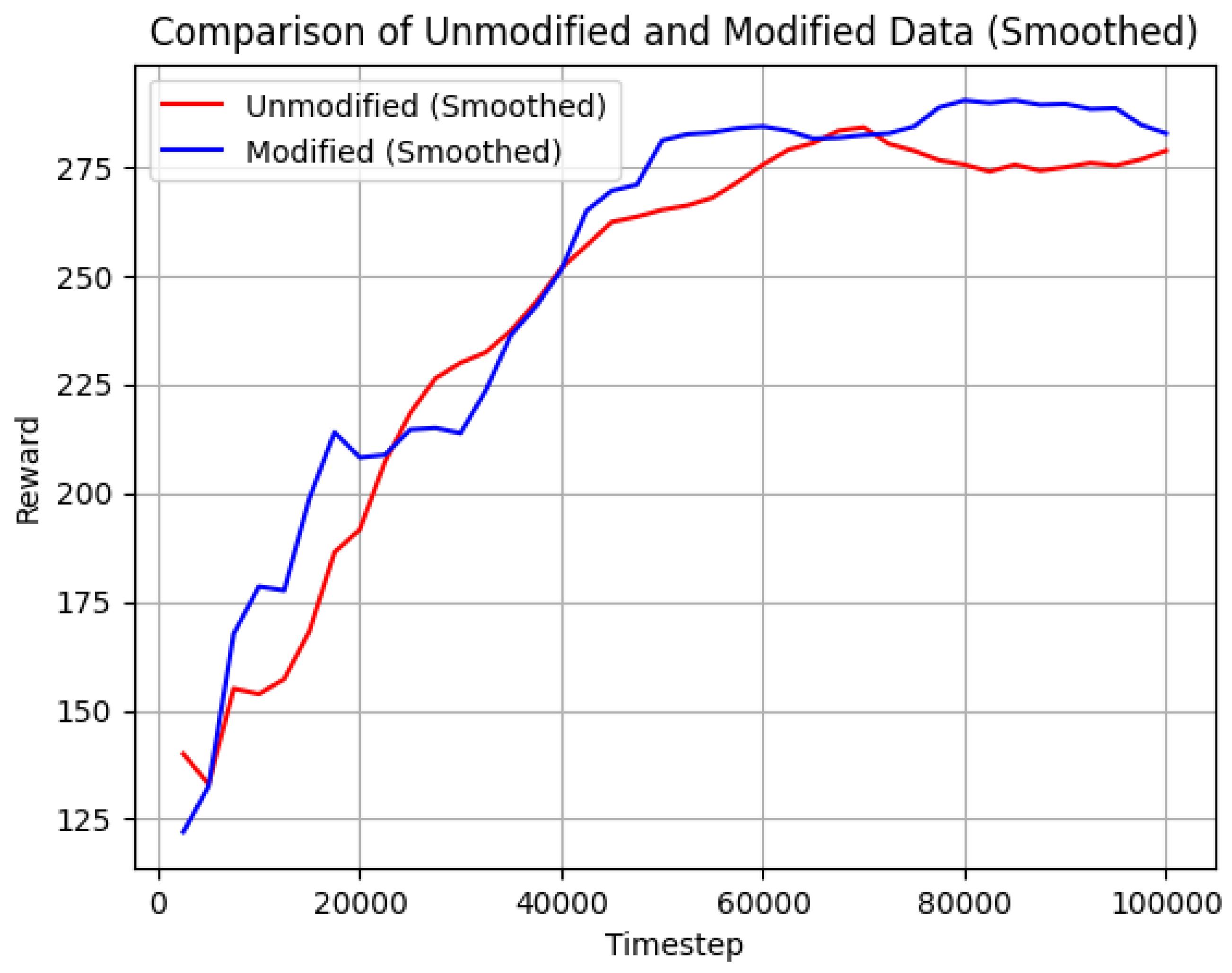
Figure 14.
RVisualization Results of the Improved SAC Algorithm
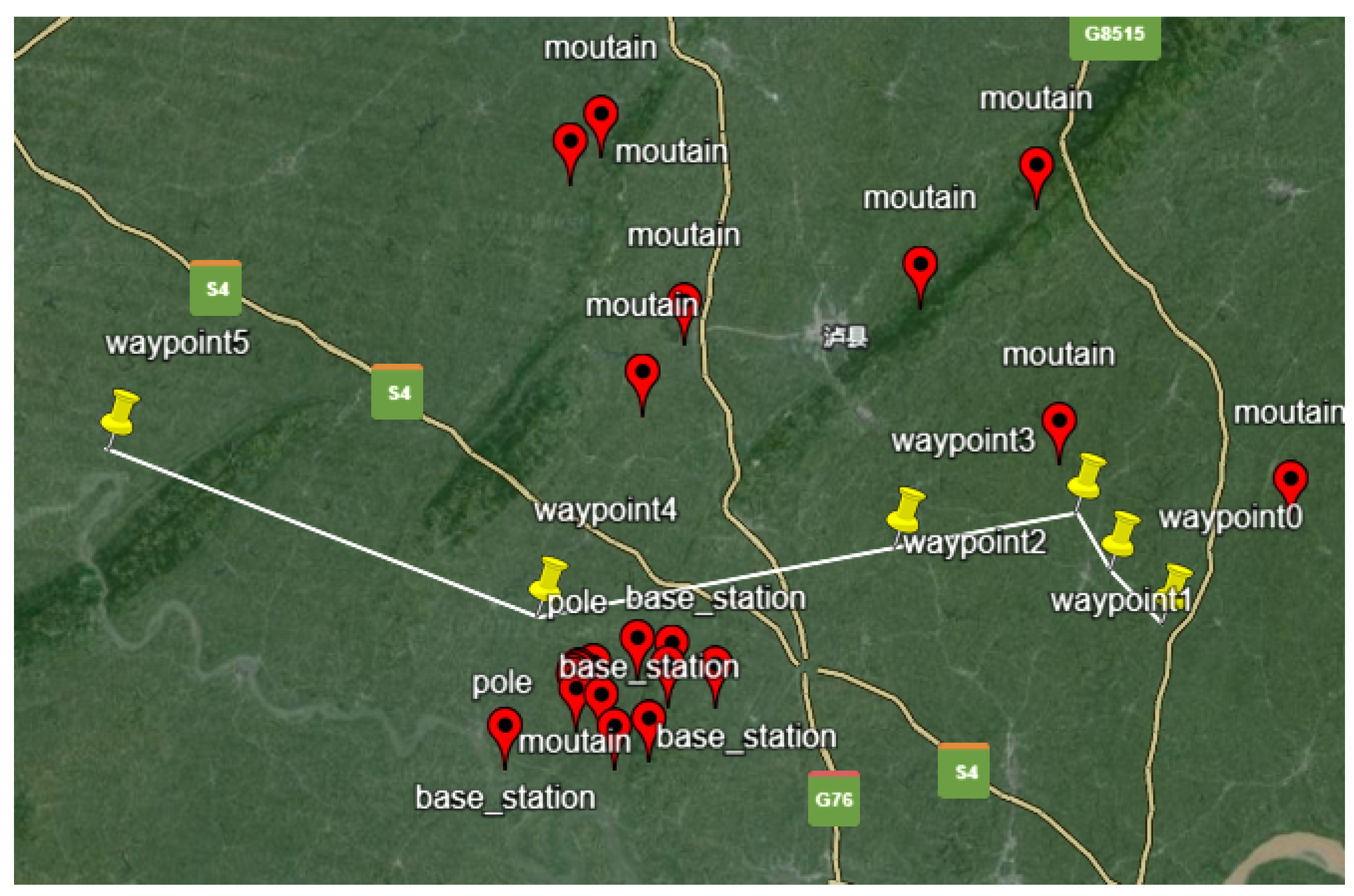
Figure 15.
Verification procedure 1
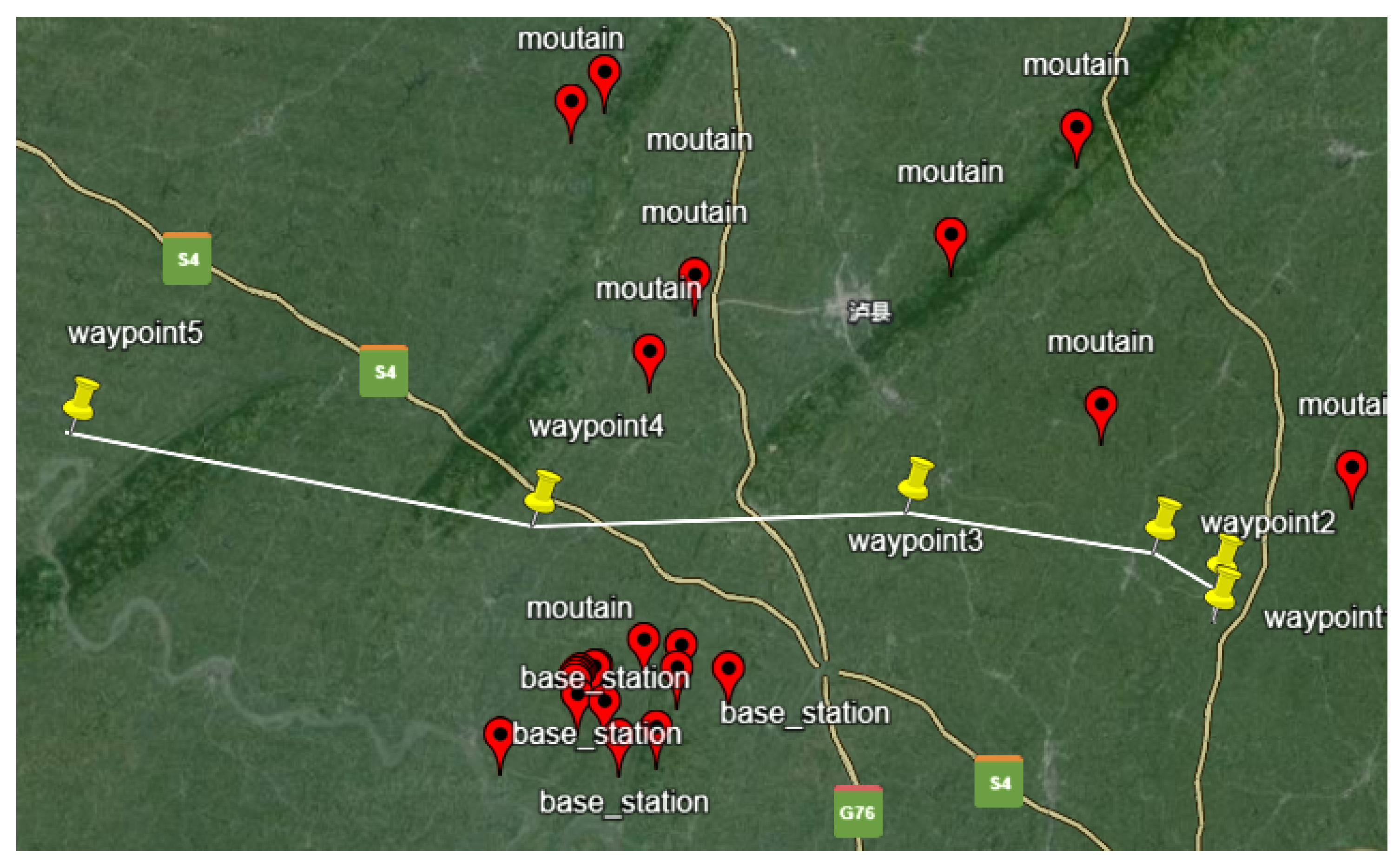
Figure 16.
Verification procedure 2
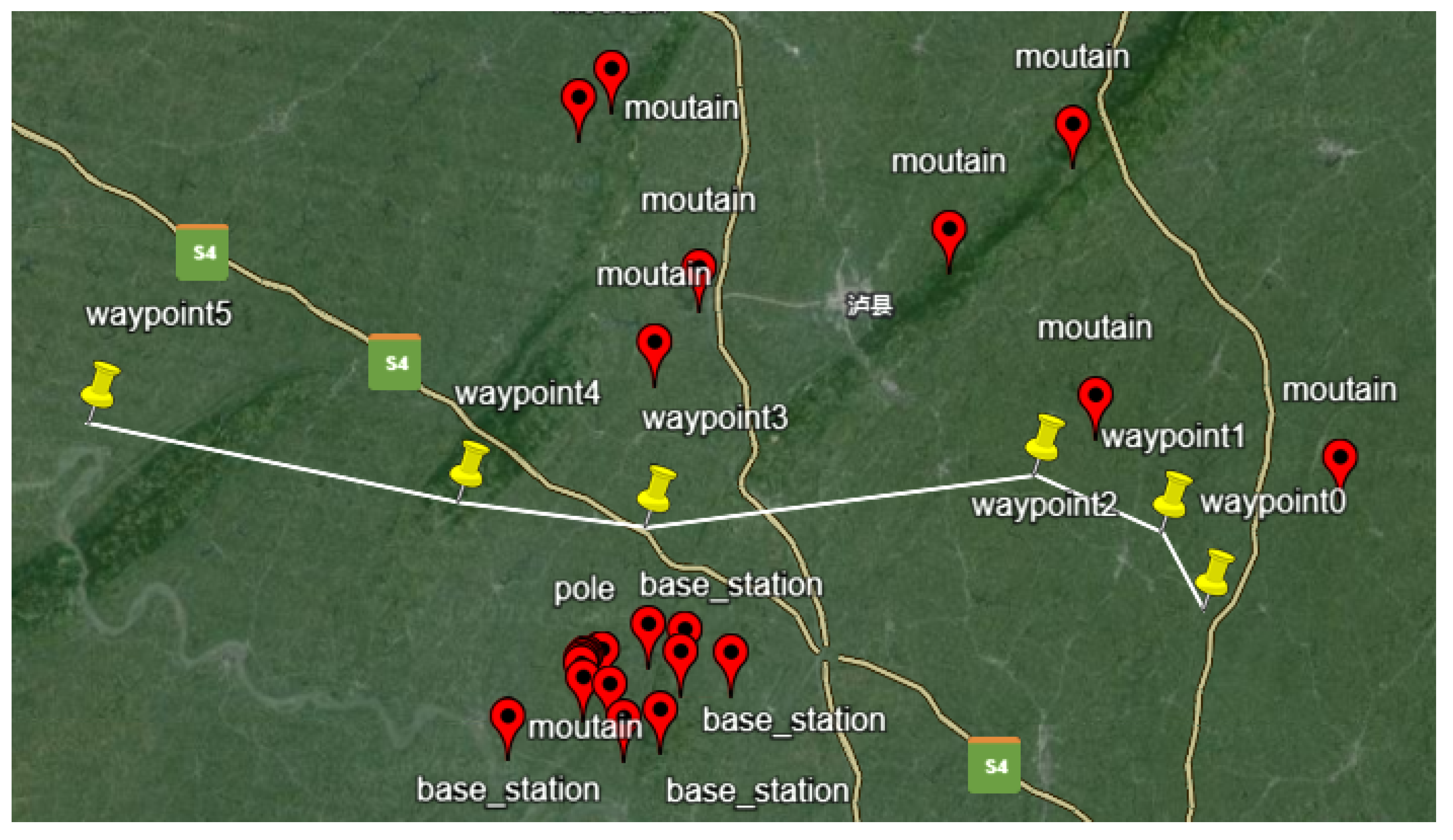
Figure 17.
Comparison of the Simulation Trajectory and Flight Path for Verification procedure 1
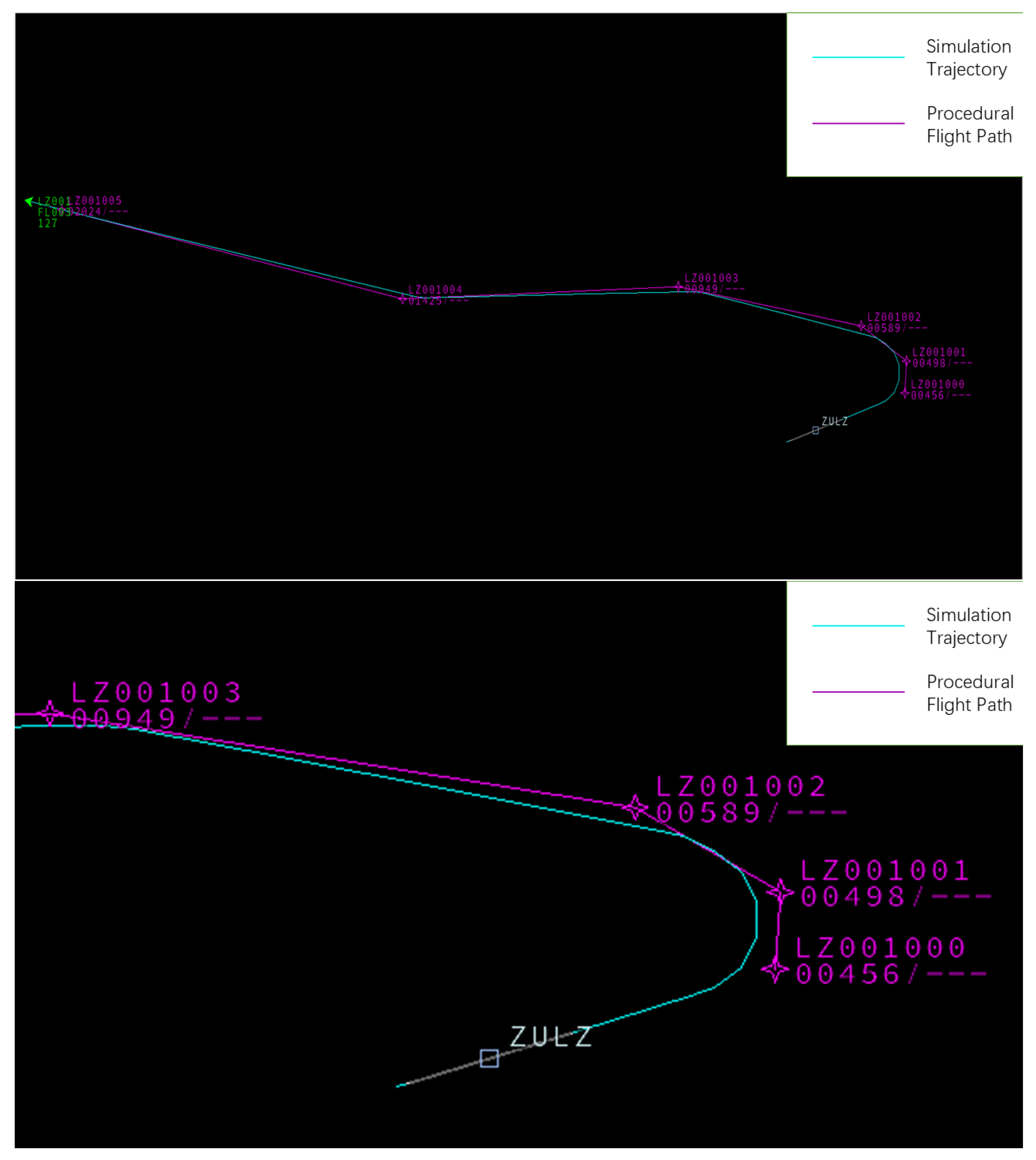
Figure 18.
Comparison of the Simulation Trajectory and Flight Path for Verification procedure 2
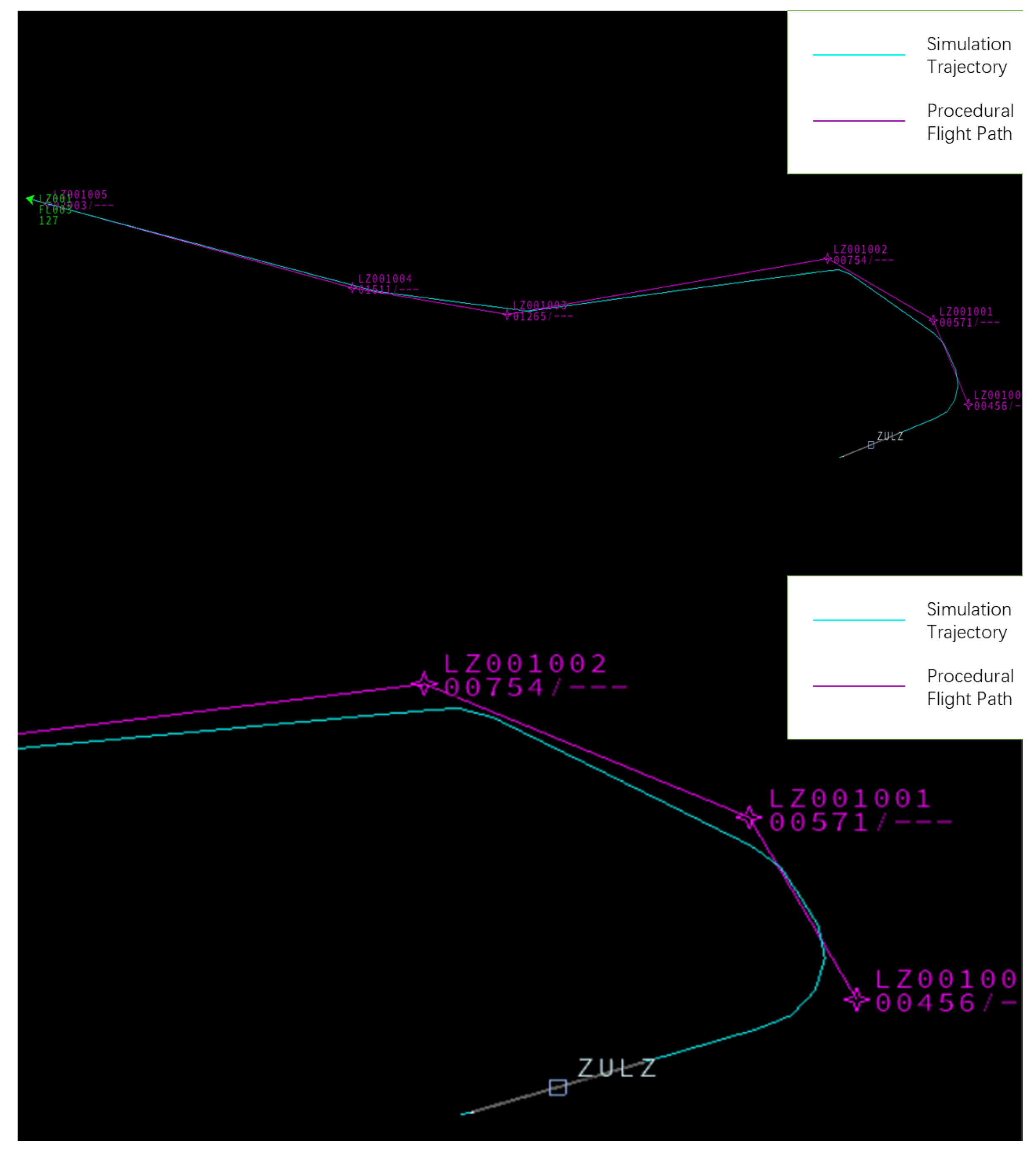
Table 2.
Luzhou Airport Information.
| Airport | Longitude | Latitude | Runway | Heading | Elevation |
|---|---|---|---|---|---|
| ZULZ | E105.46889° | N29.03056° | 07 | 75° | 335.6m |
Table 5.
Table 4-6: Multi-objective Optimization Reward Indicators and Their Value Ranges.
| Reward | Definition | Value Range |
|---|---|---|
| Safety reward, determined by the information of obstacles and the distance from the current aircraft to the obstacle. | 0-1 | |
| Angle efficiency reward, determined by the current route selection and the three turning angles of the aircraft. | 0-3 | |
| Distance efficiency reward, determined by the distance information and the length of the procedure from the current aircraft to the destination. | 0-3 | |
| Environmental noise reward, determined by the negative reward of noise. | 0-1 |
Table 6.
Comparison of Original and Improved SAC Reward Scores
| Score | Original SAC | Improved SAC | Comparison |
| Average Reward | Average Reward | ||
| 275.3 | 285.5 | +4% |
Disclaimer/Publisher’s Note: The statements, opinions and data contained in all publications are solely those of the individual author(s) and contributor(s) and not of MDPI and/or the editor(s). MDPI and/or the editor(s) disclaim responsibility for any injury to people or property resulting from any ideas, methods, instructions or products referred to in the content. |
© 2025 by the authors. Licensee MDPI, Basel, Switzerland. This article is an open access article distributed under the terms and conditions of the Creative Commons Attribution (CC BY) license (http://creativecommons.org/licenses/by/4.0/).
Copyright: This open access article is published under a Creative Commons CC BY 4.0 license, which permit the free download, distribution, and reuse, provided that the author and preprint are cited in any reuse.


