Submitted:
25 June 2025
Posted:
26 June 2025
You are already at the latest version
Abstract
Unmanned Aerial Vehicles (UAVs) are revolutionizing numerous industries, yet the complexities of executing missions in dynamic aerial environments present significant challenges. This study explores the application of Deep Reinforcement Learning (DRL) agents to address these challenges, specifically focusing on the autonomous landing of drones on maritime vessels. While conventional systems allow for automated landings, they often lack adaptability to specific locations and orientations. In contrast, DRL agents excel at learning optimal control strategies tailored to intricate tasks and diverse conditions. By mastering these strategies, DRL agents can significantly enhance the safety and efficiency of autonomous landings, paving the way for advanced high-level API integration in landing commands. This research aims to demonstrate that leveraging DRL can transform UAV operations, making them more reliable and effective in challenging environments. Ultimately, the findings have the potential to not only improve maritime operations but also extend to various other applications where precision and adaptability are paramount. This innovative approach positions DRL as a key player in the evolution of autonomous UAV technology, driving advancements in operational capabilities and safety standards. To support this research, we created a simulated environment using Unreal Engine 4.27, UAV provided by AirSim plugin and RL training facilitated by Gymnasium and Stable Baselines3.
Keywords:
reinforcement learning
; gymnasium
; Unreal Engine
; Stable baseline3
; AirSim
; UAV
; autonomous landing
1. Introduction
Unmanned Aerial Vehicles (UAVs) have undergone a profound transformation over the past decade, evolving into versatile tools that underpin a wide range of applications, from surveillance and logistics to disaster response and military operations. This evolution has been fueled by the integration of artificial intelligence (AI), which has significantly enhanced UAV capabilities in terms of autonomy, operational range, and real-time decision-making [1,2]. Despite these advancements, one of the most persistent and critical challenges in UAV operations is achieving precise and reliable autonomous landing, particularly in dynamic and unpredictable environments such as maritime vessels and urban landscapes [3]. The ability to execute safe and efficient landings is not only vital for extending mission longevity and minimizing equipment damage but also for enabling UAV deployment in complex scenarios where traditional navigation systems falter [4]. The development of AI, particularly reinforcement learning (RL), has emerged as a cornerstone in addressing these challenges. Drawing from groundbreaking achievements in gaming such as AlphaGo’s mastery of Go and StarCraft II’s multi-agent strategies deep reinforcement learning (DRL) has demonstrated remarkable proficiency in solving complex, high-dimensional decision-making problems under uncertainty [5]. These successes have spurred a wave of research applying DRL to robotics and UAV navigation, domains where adaptability to diverse and evolving conditions is essential [6]. Traditional autonomous landing systems, which often rely on Global Navigation Satellite System(GNSS-based) navigation, visual markers, or heuristic-based controllers, are effective in controlled settings but struggle to cope with external disturbances such as wind gusts, moving platforms, or sensor noise [7]. In contrast, DRL empowers UAVs to autonomously learn optimal landing strategies through iterative trial-and-error interactions with their environment, eliminating the need for exhaustive manual tuning [8].
The limitations of conventional landing methods are particularly evident in specialized applications. In maritime environments, UAVs must contend with dynamic factors such as ship motion, wave-induced perturbations, and adverse weather conditions, all of which demand robust and adaptive landing solutions [9]. Similarly, dynamic landing scenarios, such as those involving moving platforms or turbulent environmental conditions, require UAVs to exhibit adaptive control capabilities, ensuring safe touchdown despite non-stationary targets and real-time perturbations. This highlights the importance of precision landing agents capable of learning robust behaviors in complex, time-varying environments[10]. DRL offers a promising framework to tackle these issues by enabling UAVs to refine their landing trajectories in real time, adapting to unpredictable variables [4]. For instance, prior work has demonstrated that DRL can outperform classical control approaches, such as proportional-integral-derivative (PID) and model predictive control (MPC), in handling dynamic conditions, offering greater flexibility and resilience [2].
A key strength of DRL lies in its ability to leverage advanced algorithms like Proximal Policy Optimization (PPO) and Deep Q-Networks (DQN), which enhance the generalization of landing strategies across diverse scenarios [3]. These algorithms allow UAVs to develop policies that are less dependent on predefined rules, making them well-suited for tasks requiring high adaptability. However, a significant barrier to widespread adoption is the challenge of transferring DRL-trained policies from simulated environments to real-world deployments. Discrepancies arising from sensor noise, hardware limitations, and unforeseen environmental factors often degrade performance in physical settings [7]. To address this, high-fidelity simulation platforms like Unreal Engine and AirSim have been developed to replicate real-world physics and environmental dynamics, providing a realistic training ground for UAVs. Complementary techniques such as domain randomization, introduce variability into training scenarios e.g., altering lighting, wind patterns, or platform motion, enhancing the robustness of DRL models for real-world applications [11]. Beyond individual UAV performance, the rise of multi-agent systems has opened new avenues for innovation. UAV swarms, enabled by DRL and swarm intelligence, facilitate cooperative landing strategies that optimize safety and efficiency in constrained or contested spaces [9,12]. Recent studies have explored how DRL can enhance swarm coordination, allowing UAV fleets to dynamically adjust their behavior based on real-time environmental feedback [13]. These advancements underscore the potential of DRL to revolutionize not only individual UAV operations but also large-scale autonomous systems.
Related work further illuminates the trajectory of DRL in UAV autonomy. Early efforts focused on basic navigation and obstacle avoidance, with foundational contributions demonstrating the feasibility of RL in robotic control [4]. Subsequent research expanded to complex tasks like agile flight and collision avoidance, leveraging deep neural networks to process high-dimensional sensor data [6,7]. More recently, attention has shifted toward specialized landing scenarios, such as maritime and urban operations, where precision and robustness are paramount [10]. Innovations in training frameworks, such as the use of Gymnasium and Stable Baselines3, have streamlined the development of DRL models, enabling systematic evaluation across diverse conditions.
This research aims to advance deep reinforcement learning (DRL) methods for autonomous UAV landing in dynamic maritime environments, with an emphasis on vision-based control and adaptive decision-making. The broader applicability of the proposed framework extends to several real-world domains. In logistics, improved landing precision can enhance the efficiency and reliability of drone-based delivery systems, particularly in cluttered or constrained landing zones. In disaster response, the ability to autonomously land in unstructured or hazardous environments can facilitate critical access to otherwise unreachable areas. Moreover, defense applications may benefit from increased landing robustness in contested or GNSS-denied environments, where rapid and accurate deployment is operationally essential.
2. Materials and Methods
The RL Based Auto Landing System Architecture in this study is described in Figure 1.
System Architecture:
-
Simulation Environment:
- –
- Simulation Engine: Unreal Engine 4.27, providing high-fidelity, physics-based simulation for accurate representation of real-world environments [14].
- –
- Simulation Plugin: AirSim, plugin for Unreal Engine, enabling interaction with aerial and ground vehicles within the simulated environment, including sensors, control mechanisms, and environmental dynamics[15].
- Reinforcement Learning Framework: Gymnasium, An extended, open-source version of OpenAI Gym for developing, managing, and testing reinforcement learning environments. Gymnasium is fully compatible with diverse algorithm packages and supports custom environments[16].
- Algorithm Package: Stable Baselines 3, A Python library of proven and stable reinforcement learning algorithms, including PPO, DQN, A2C, and SAC, optimized for Gymnasium-compatible environments[17].
- System runtime environment: on-premise machine, Google-Colab[18].
- Additional Reinforcement Learning Activities: Unified Training Pipeline for High-Fidelity Reinforcement Learning, Reward Function Engineering and Hyperparameter Tuning.
The system architecture integrates all components into a cohesive framework for training a deep reinforcement learning agent to perform autonomous UAV landings on maritime vessels. Unreal Engine 4.27 and AirSim jointly provide a high-fidelity simulation environment with time acceleration capabilities, simulating UAV flight dynamics via Pixhawk/PX4 and replicating maritime conditions using physics-based vessel models. The environment is interfaced with Gymnasium to enable seamless integration with Stable Baselines3, which implements the Proximal Policy Optimization (PPO) algorithm for policy learning. The system has been evaluated across both on-premise hardware and a hybrid setup combining local infrastructure with cloud-based computation (Google Colab), offering flexibility in training scalability and runtime acceleration.
3. Problem Formulation
To train a DRL agent for autonomous UAV landing on a moving maritime vessel, we model the task as a Markov Decision Process (MDP), formally defined by , as illustrated in Figure 2, where:
- S: State space, representing the UAV’s observations of itself and its environment.
- A: Action space, defining the discrete set of actions available to the UAV.
- R: Reward function, providing scalar feedback that guides the agent toward the goal.
- T: State transition function, governing the environment’s dynamics and how the agent’s actions lead to new states.
- : Discount factor, used to prioritize long-term rewards over immediate gains.
3.0.1. State Transition Function (T)
In the context of our simulation environment, the transition function is not explicitly defined as a probability distribution. Instead, it is implicitly realized through the physics and simulation engine of Unreal Engine 4.27 via the AirSim plugin. At each timestep:
- The agent selects an action .
- The simulator applies this action to the UAV through physics-based updates.
- The environment evolves based on the applied control and underlying dynamics (wind, motion of the ship if applied).
- A new state is returned as a result of these transitions.
Thus, T is implemented through the interaction loop of our Gymnasium environment, encapsulating both deterministic and stochastic elements of the UAV’s real-world-like dynamics.
3.0.2. Discount Factor ()
We use a discount factor of , which balances short-term rewards with long-term objectives, encouraging the UAV to plan actions that lead to stable and successful landings over time.
3.1. Goal
The objective of this research is to develop a control policy that enables the UAV to autonomously land on the vessel’s deck with high precision and reliability. A landing is considered successful if the UAV:
- Reaches a target landing zone within a specified positional and angular tolerance.
- Maintains a safe descent velocity.
- Avoids collisions or unstable control maneuvers.
This formulation provides a structured foundation for DRL training, enabling the agent to learn optimal control strategies under complex dynamic conditions.
3.2. Environment Reset Function
To ensure diverse training conditions and prevent overfitting to a fixed configuration, we implement a reset() function within the environment. This function is invoked at the beginning of each episode and performs the following tasks:
- Randomly repositions the UAV (drone) to a valid starting location in three-dimensional space, typically above or near the vessel within a predefined safe radius.
- Randomly initializes the position and orientation of the landing platform -the vessel.
- Resets the drone’s velocity and orientation to default values to ensure consistent initial conditions for learning.
- Returns the initial observation state to the reinforcement learning agent for the new episode.
This randomized reset strategy introduces environmental stochasticity, which is critical for training generalizable policies capable of handling real-world uncertainties.
3.3. Observation State Space (S)
The state at time t is represented as:
where:
- - are the UAV velocities along the x, y, and z axes.
- h - is the height of the UAV.
- - is the distance between the UAV and the ship.
- c - indicates whether a collision has occurred (binary).
- - is the distance from the object in front of the UAV.
- image - the visual observation captured by the front camera in First Person View (FPV) mode, with a resolution of 416×416×3.
- Depthimage An optional additional depth matrix observation can be added as a fourth channel to the vision image in FPV mode, with a resolution of 416×416×1, not implemented in this research but tested.
This state information is obtained from the AirSim simulation environment and sensors. AirSim offers various APIs for controlling the drone, such as moveByAngleThrottleAsync, moveByVelocityBodyFrameAsync, moveByRollPitchYawThrottleAsync, etc. In this study, we utilize the moveByVelocityAsync API, which commands the drone using linear velocities and yaw.
3.4. Action Space (A)
The UAV’s action space is discretized into 9 actions, each corresponding to a small incremental change (delta) applied to one of the control axes: translational velocities () or yaw rate. This reflects the physical constraint that a drone cannot instantly change its velocity or orientation due to inertia and actuator response limitations. Rather than specifying absolute control values, each action modifies the current control state by a fixed delta (e.g. ). In the default setup, only one control axis is affected per action step, which simplifies training and encourages gradual, stable maneuvers.
Formally, the discrete action space is defined as:
where each represents a delta adjustment to a specific control axis. A complete mapping from action indices to control deltas is provided in Section 4.2.1.
Alternatively, one can define an action strategy that applies simultaneous (parallel) delta adjustments across all control axes at each timestep. This parallel discrete approach enables coordinated control across multiple dimensions simultaneously.
Alternatively, a continuous control strategy can be employed, where the deep neural network (DNN) directly outputs continuous action values in the range for each control axis. This allows for smooth and fine grained control but increases the complexity of the policy learning problem. Both strategies parallel discrete and continuous action offer expressive control capabilities, and the choice between them depends on the specific task requirements and training stability considerations.
3.5. Reward Function (R)
The reward function is designed to reflect the high-level objectives of the autonomous landing task, promoting safe, precise, and efficient behavior throughout the UAV’s approach and descent. It integrates both positive incentives for desirable actions and penalties for hazardous or inefficient behavior, ultimately guiding the agent toward successful landings on the vessel deck.
Key factors considered in the design of the reward signal include:
- Proximity to the target landing zone.
- UAV’s height above the ocean.
- UAV’s velocity magnitude.
- Correct alignment with landing markers (ARUCO detection).
- Distance to nearby obstacles.
- Collision events.
- Elapsed mission time.
- Successful completion of the landing.
These elements are combined to provide the agent with structured feedback at each timestep, with a terminal reward granted upon successful landing. The detailed formulation of the reward function is presented in Section 4.2.
4. Research Approach
To investigate and validate the proposed autonomous landing framework, we adopt a simulation-based research approach that integrates high-fidelity environmental modeling, reinforcement learning infrastructure, and advanced training algorithms. This modular setup allows for controlled experimentation while maintaining realism in UAV dynamics and maritime conditions.
The following subsections detail the key components of our system:
- Simulation Environment: Built using Unreal Engine 4.27 and AirSim to replicate realistic ship motion and UAV flight dynamics.
- Environment Integration: Gymnasium interface to connect the simulation with standard reinforcement learning frameworks.
- Learning Algorithms: Implementation and training using Stable-Baselines3 for policy optimization.
4.1. Simulation Environment
To train and evaluate the UAV landing policy under realistic conditions, we developed a high-fidelity simulation environment using Unreal Engine 4.27 in combination with the Microsoft AirSim plugin (Figure 3). This platform provides a physics-accurate, visually realistic environment for simulating aerial robotics tasks, including perception, control, and navigation. The simulation scene includes a maritime vessel with a designated landing pad, designed to emulate the dynamics and constraints of shipboard landings. The UAV model is equipped with configurable sensors and control interfaces, including front-facing RGB camera, optional depth input, and inertial measurements.
Features of the simulation setup include:
- Realistic UAV Dynamics: Accurate flight physics, motor response, and environmental drag modeled by AirSim’s flight controller.
- Custom Maritime Scene: A custom ship deck environment placed in an open sea scenario, with spatial constraints relevant to real-world landing conditions.
- Camera Sensor Model: The UAV uses a forward-facing RGB camera in First Person View (FPV) mode with resolution, with optional support for a fourth depth channel.
- Reset Functionality: Each episode begins by resetting the UAV and vessel to randomized positions and orientations within predefined bounds, ensuring diversity across training episodes.
- APIs for Control and Sensing: The UAV is controlled using AirSim’s moveByVelocityAsync API, allowing direct velocity-based commands in 3D space along with yaw angle adjustments.
- Weather Control: The simulation supports dynamic weather manipulation, including fog, rain, wind strength, snow and leaves , which can be adjusted to test model robustness under varying visual and environmental conditions.
- Stable Simulation Mode: To ensure deterministic behavior during reinforcement learning, the simulation can be run in a frame-locked, physics-consistent mode that eliminates external variability during training.
- Accelerated Clock Speed: The simulation clock can be accelerated beyond real-time, enabling faster-than-real-world training cycles while maintaining physical consistency.
This simulation framework enables reproducible experimentation in a controlled but realistic setting, forming the foundation for the reinforcement learning pipeline described in the following sections.
4.2. Environment Integration – UEAIRSIM Env Class
To enable reinforcement learning within a physics-realistic maritime landing simulation, we developed a custom environment named UEAIRSIM, which integrates Microsoft AirSim and Unreal Engine 4.27 Ocean Map. The environment adheres to the Gymnasium API specification, allowing seamless compatibility with widely used DRL frameworks such as Stable-Baselines3.
4.2.1. Action Space and Mapping
For simplicity, we define a discrete action space consisting of 9 control primitives that govern the drone’s translational and yaw dynamics. Each action index maps to a specific motion directive, which is executed using AirSim’s moveByVelocityAsync interface. The action space is defined using the Gym API as:
where each discrete action corresponds to a predefined control primitive. The full mapping of action indices to control commands is presented in Table 1.
Each action applies a small delta change to the corresponding control channel, either linear velocity or yaw rate, within predefined bounds ( m/s, with m/s). These values are clipped as necessary to respect UAV dynamics and ensure smooth transitions.
Alternatively, for continuous control, the action can be defined as a 4 dimensional vector:
corresponding to . This approach allows simultaneous adjustments across all control axes and supports fine-grained maneuvering. The scaled values define velocity commands within the range m/s for translation and deg/s for yaw rate.
4.2.2. Observation Space
The agent’s observation is represented as a dictionary composed of multiple sensor and state features. The observation space is defined using the Gym API as:
self.observation_space = Dict({
’velocities’: spaces.Box(low=-1, high=1, shape=(3,), dtype=np.float32),
’height’: spaces.Box(low=-1, high=1, shape=(1,), dtype=np.float32),
’distanceFromBoat’: spaces.Box(low=0, high=1, shape=(1,), dtype=np.float32),
’collision’: spaces.Box(low=0, high=1, shape=(1,), dtype=np.uint8),
’image’: spaces.Box(low=0, high=255, shape=InputImgShape, dtype=np.uint8),
’FrontDistance’: spaces.Box(low=0, high=1, shape=(1,), dtype=np.float32),
})
where:
The observation space includes the following components:
- RGB Image: Multi-modal image data captured from the UAV’s first-person view (FPV) camera, with dimensions . Each modality contributes a standard RGB image tensor of shape , and may include additional representations such as infrared (IR) imagery, semantic masks (e.g., no-fly zones), or other sensor-derived visual channels. For simplicity, we set , corresponding to a single RGB image.
- Linear Velocities: A normalized vector representing the UAV’s linear motion in three directions: .
- Height: The UAV’s normalized height above a reference point (vessel deck). Represented as a scalar value in the range .
- Distance from boat: The normalized Euclidean distance between the UAV and the target vessel. Scalar in the range .
- Collision Flag: A binary indicator (0 or 1) that signals whether the UAV has collided with an object or surface.
- Frontal Obstacle Proximity: A normalized scalar indicating the distance to the nearest object in the UAV’s frontal flight path, useful for low-level obstacle avoidance. Value lies in .
This hybrid observation design facilitates spatiotemporal learning through both internal and external feedback. It also provides the agent with richer contextual information, enabling more effective reasoning about the environment.
4.2.3. Reset Behavior
Upon invoking reset(), both the UAV and the vessel are initialized to randomized positions and orientations within a maximum radius defined by the simulation parameters. This ensures diverse starting conditions and promotes robust policy learning. The UAV is also assigned an initial velocity vector with a randomized direction to break symmetry in early episodes. In addition, key observation state variables are reset, including Collision Status, Cumulative Reward, and Timestep Counters.
The initial observation returned includes:
- Stacked Image Tensors from the UAV’s Onboard Camera
- Feature Vectors such as Velocity, Height, Distance to the vessel, etc.
- Metadata including Episode Count, Cumulative Reward, and Timestep Index
Randomization during environment reset plays a critical role in improving the generalization and robustness of the learned policy. By exposing the agent to a wide variety of initial configurations, both in terms of spatial positioning and dynamic orientation, it becomes less prone to overfitting on specific trajectories or start conditions. This diversity encourages the agent to develop adaptive and resilient strategies that can perform reliably under real-world variability and unforeseen disturbances.
4.2.4. Step Dynamics and Environment Logic
Each call to step(action) follows a synchronized sequence designed to maintain simulation determinism and ensure stable learning. The agent’s discrete (or continuous) action is first interpreted and mapped into velocity and yaw commands through the interpret_action() function. Once the action is determined, the simulation is briefly unpaused to allow physics updates, during which a velocity command is issued to the UAV using AirSim’s moveByVelocityAsync() API interface. This command is executed under a time accelerated setting, typically scaled by a factor of x40/×100 or more, to simulate faster UAV dynamics and improve training efficiency. Immediately after the UAV executes the commanded motion, the simulation is paused again to preserve a consistent world state. At this point, RGB images and onboard sensor data are retrieved and organized into a structured observation. A scalar reward is then computed based on the UAV’s updated state and sensory feedback, and a check is performed to determine whether a terminal condition has been met. This freeze–execute–freeze scheme guarantees frame aligned data collection, which is critical for reproducible transitions and stable training in deep reinforcement learning workflows.
4.2.5. Reward Function
The reward function serves as a critical mechanism for encoding task objectives into numerical feedback, allowing the agent to learn meaningful behaviors through trial and error. In this environment, the reward signal is designed as a weighted composition of multiple behavior-shaping components, with the overarching goal of guiding the UAV to safely and efficiently land on a vessel deck using onboard visual and internal sensor feedback.
This reward function blends shaped and sparse elements: shaped rewards accelerate early learning through continuous feedback, while sparse terminal bonuses enforce the full completion of the landing objective. This hybrid design balances exploration efficiency with policy optimality, a common strategy in complex reinforcement learning tasks.
The main reward components include:
- Time Penalty: A small negative reward is applied at every step to discourage prolonged hovering and encourage time-efficient decision making. This value is estimated as . To encourage extensive exploration during early training while promoting efficient task completion as learning progresses, we introduced a dynamic scheduling mechanism for the episode length limit. Specifically, the MaxSteps parameter, which defines the maximum number of time steps per episode, was initialized to 4,500 steps. As training advanced and the agent began to consistently complete episodes in fewer steps, the MaxSteps value was gradually decreased. This decay continued until it reached a minimum threshold of 700 steps. This adaptive mechanism allowed the agent to benefit from prolonged exploration in the initial phase, while progressively constraining the horizon to favor rapid and precise landings once the policy matured.
- Obstacle Avoidance: The agent receives a penalty inversely proportional to its distance from frontal obstacles, promoting conservative maneuvering near the vessel’s structure and avoiding sudden collisions. This capability is predominantly acquired through the RGB image returned by the environment.
- Distance to Vessel: A shaped penalty signal encourages the UAV to approach the vessel’s deck. The normalized distance-based reward is defined as:where is the Euclidean distance between the UAV and the center of the landing zone, is the maximum measurable distance within the simulation bounds, and MaxTimeSteps is the upper limit on episode length. This normalization ensures that the distance penalty remains small and consistent across different episode durations.
- Object Detection Bonus: Semantic detections of key visual cues, such as the VesselBack region or the ArUco landing marker (AR),contribute to a positive shaped reward same as time penalty. While detecting the general structure of the vessel’s rear can be sufficient for basic navigation, our research specifically leverages the ArUco marker to ensure precise alignment with the front edge of the vessel’s deck. The ArUco detection enables the UAV to maintain a target-relative orientation and distance prior to descent, supporting robust, vision-guided landings.
-
Successful Landing Bonus: A large terminal reward is granted when the UAV satisfies all successful landing conditions:
- –
- Position is within the physical boundaries of the landing pad.
- –
- The AR landing marker is visually detected with sufficient confidence.
- –
- Descent velocity is below a safe landing threshold <0.5m/s.
-
Unsuccessful Landing Penalty: A terminal penalty of is applied in all cases where the UAV fails to achieve a safe landing. This includes:
- –
- Collisions with any object other than the designated landing deck—including the vessel’s body, ocean surface, or onboard obstacles.
- –
- Exiting the designated operational boundaries.
- –
- Exceeding the maximum allowed flight altitude.
- –
- Failing to complete the landing within the predefined time horizon.
Each of these conditions results in immediate episode termination and is intended to discourage unsafe or inefficient behavior.
The total reward at each timestep is formulated as a weighted sum over all reward components:
where represents the reward signal (e.g., vessel alignment, AR marker detection, time penalty, collision, landing success, etc.), and is the corresponding scalar weight that controls its contribution to the overall reward. The number of components N depends on the specific structure of the reward function, which is designed to balance guidance, safety, and task success. we can assume that .
In reinforcement learning, the agent aims to maximize the expected cumulative return over time, defined as:
where is the return at timestep t, is the total reward received k steps after t, and is the discount factor that weights the importance of future rewards. The reward function defined above serves as the per-timestep scalar signal within this temporal framework, directly influencing the optimization of the policy through gradient-based methods.
An episode is terminated when the UAV either lands successfully on the vessel deck, collides with an obstacle or falls into the ocean, exceeds the predefined maximum number of simulation steps, or flies beyond the allowed spatial boundaries of the environment. This termination logic, when combined with the reward function, defines the structure of the exploration space and directly influences the policy gradient signal used during learning. The design of this reward function reflects careful tradeoffs between ’shaped rewards’- for guided learning and sample efficiency and ’sparse incentives’- to enforce the complete satisfaction of mission objectives. Such a design also encourages multi stage task reasoning approach, align, descend, and touch down aligned with real world UAV operation procedures.
4.3. Learning Algorithms
This study adopts a modular learning architecture that decouples the simulation environment from the reinforcement learning (RL) algorithm, facilitating flexible experimentation. The simulation is based on Microsoft AirSim integrated with Unreal Engine, customized to simulate maritime conditions for UAV landings on dynamic vessel decks. The RL agent is trained using the Stable-Baselines3 framework, with a focus on the Proximal Policy Optimization (PPO) algorithm due to its robustness and compatibility with high-dimensional observation spaces.
Initially, a distributed training setup was investigated, wherein the AirSim simulation was executed on a local workstation while the learning algorithm was run on a remote Google Colab instance, Figure 1. This architecture aimed to exploit the GPU acceleration provided by Colab while offloading simulation workloads to local hardware. However, this approach introduced significant instability due to latency and simulation speed mismatch. Specifically, the AirSim environment was configured with a time acceleration factor of to , allowing rapid simulation of UAV dynamics for efficient policy learning. In this setup, the typical network delay between the local simulator and the Colab agent was approximately 60 milliseconds non constant. This delay, although negligible in real-time systems, became substantial when combined with the simulation acceleration, resulting in a breakdown of synchronization between action commands and environmental observations. Furthermore, AirSim internally employs a release–step–pause cycle to ensure deterministic simulation. Any communication latency between steps thus led to stale observations, delayed actions, and, in practice, an unstable training process with poor convergence and inconsistent behavior.
To mitigate these issues, we transitioned to a fully local training pipeline. Both the simulation environment and the reinforcement learning agent were hosted on the same workstations environment with low latency Ethernet connection, eliminating network-induced lag and maintaining a synchronized control-feedback loop. This setup enabled reliable and reproducible training by preserving the determinism of each simulation step and ensuring real-time feedback during the training process. Due to local station scheduling preferences, training tasks were automatically limited to 24\48 hour intervals, a common constraint in high performance computing environments. This experience underscores the importance of minimizing control and observation latency in high-frequency environments and highlights the necessity of localizing both simulation and learning components when working with accelerated time dynamics. Specifically, in the case of AirSim, which requires explicit simulation pausing after each action (via the pause command), the system becomes highly sensitive to network delay. This tight coupling between control input and simulator response makes remote training impractical under latency constraints. However, in environments that natively execute an actions and automatically pause at the end of each step thus enforcing frame-level determinism, remote component separation may still be feasible. Such simulators inherently decouple execution from frame timing and can better tolerate the asynchronous nature of remote computation. Therefore, the choice to run the simulation and learning components on the same machine should be informed by the simulator’s control model and real-time synchronization requirements.
The environment was integrated into the RL pipeline using the Gymnasium API and further wrapped with the VecFrameStack and Monitor wrappers provided by Stable-Baselines3 to enable frame stacking and episode-level logging. Observations comprised both stacked RGB images from the UAV’s onboard camera and structured proprioceptive features (velocity, altitude, distance to target, and collision indicators etc.).
The PPO agent was trained using the following hyperparameters:
- Learning rate:
- Discount factor:
- Generalized Advantage Estimation:
- Number of steps per rollout: 8192
- Batch size: 64
- Number of epochs per update: 10
- Clipping parameter: 0.2
- Entropy coefficient: 0.01
To effectively learn a policy capable of controlling the UAV in complex maritime scenarios, the training procedure utilized the MultiInputPolicy architecture, which enables simultaneous processing of both visual (image-based) and non-visual (feature-based) modalities. This policy structure is particularly critical for tasks that require integrating spatial perception from camera input with numerical telemetry such as altitude, velocity, and distance metrics. To enhance visual perception and facilitate faster convergence, a YOLOv3 object detection model was independently trained prior to reinforcement learning to detect key maritime features, including the vessel, its deck, and a fiducial ArUco marker placed on the landing area. This pre-trained detection network was used to extract high-level latent representations of the scene, which were then passed as part of the visual input to the policy network. Incorporating this structured latent space into the policy learning pipeline provided two significant advantages. First, it improved reward feedback by enabling the agent to more accurately localize and align with the landing platform, resulting in higher quality state representations. Second, it significantly reduced training time by offloading low-level visual feature learning to the pre-trained detector, allowing the policy network to focus on high level decision making. This modular design effectively decouples perception from control, accelerating policy convergence while maintaining task robustness.
To ensure training reproducibility and enable fault-tolerant experimentation, model checkpoints were periodically saved using the CheckpointCallback. In parallel, quantitative policy evaluation was performed every 25,000 environment steps via the EvalCallback, allowing the monitoring of policy generalization over fixed test scenarios. Training metrics, including episodic reward, policy entropy, and explained variance, were logged and visualized using TensorBoard. These diagnostics facilitated the detection of learning instabilities and the verification of long-term training convergence.
The Proximal Policy Optimization (PPO) algorithm was trained for over 160 million timesteps to optimize the stochastic policy [19]. While the policy demonstrates good convergence and exhibits stable performance across a wide range of scenarios, it has not yet achieved consistently precise landings under all environmental conditions. This indicates that, although significant progress has been made, additional training is necessary to reach a level of precision and robustness suitable for real-world deployment.
- Initialization: The agent’s policy was initialized with randomized weights. Each training episode began from diverse environmental conditions, including UAV heights sampled uniformly from 5 to 20 meters, randomized relative positions between the UAV and the ship, and initial distances from the landing target up to 160 meters. This variability promotes policy generalization and avoids overfitting to narrow state distributions.
-
Policy Optimization: The PPO algorithm maximizes a clipped surrogate objective:where is the probability ratio between the new and old policies, and is the advantage estimate at time t. The clipping threshold was set to , as recommended in the original PPO formulation.Advantage estimates were computed using Generalized Advantage Estimation (GAE), which balances bias and variance through the temporal decay factor :where represents the temporal difference (TD) error and is the discount factor.
- Evaluation: Policy performance was evaluated every 25,000 timesteps on a set of held-out test scenarios. These scenarios were sampled with varied initial UAV positions and environmental conditions, ensuring that the evaluation metrics reflected true generalization rather than memorization of specific trajectories.
5. Results and Discussion
The research results demonstrate the learning dynamics and policy convergence of the PPO agent developed for autonomous UAV landing. This section presents a detailed analysis of key performance metrics that capture both training stability and task efficiency. Specifically, we report the evolution of:
- Explained variance, to assess the accuracy of the value function.
- Entropy loss, to monitor the policy’s exploration behavior.
- Average episode length, as an indicator of task completion efficiency.
- Mean evaluation reward, to measure overall task success and policy improvement.
These metrics were tracked throughout the training process, as shown in Figure 4 and Figure 5, to illustrate the learning dynamics, policy convergence, and stability achieved by our PPO-based agent. The following graphs detail the progression of key performance indicators over time and demonstrate the effectiveness of the training strategy.
Explained Variance: The left panel of Figure 4 shows the evolution of the explained variance, which measures how well the learned value function approximates the actual empirical returns . A value of 1.0 indicates perfect prediction, while values below zero imply poor generalization. For the PPO_AutoLanding runs, the explained variance increases steadily over time, reaching values above 0.9, suggesting highly accurate value estimation. This indicates that the critic network is effectively learning to approximate the return distribution.
Entropy Loss: The right panel of Figure 4 presents the entropy loss curve, which captures the stochasticity of the policy . A more negative entropy loss indicates higher randomness in action selection, while values closer to zero reflect a more deterministic policy. Over the course of training, the entropy loss increases, demonstrating the expected reduction in policy entropy as the agent converges and shifts from exploration to exploitation. The PPO_AutoLanding runs maintain an overall increasing entropy trend throughout training, with a brief drop near the end. This drop is followed by a recovery to higher entropy levels, likely due to a learning rate adjustment. This behavior indicates a more balanced exploration strategy, which may have contributed to their superior performance in reward optimization and policy stability.
Episode Length: As shown in Figure 5, the left panel illustrates the average episode length (eval/mean_ep_len) throughout the training process. At the beginning of training the episode length is high, exceeding above 4,000 steps, indicating inefficient or random policies. Over time, the PPO_AutoLanding agent exhibits a sharp decline in episode length, converging to fewer than 250 steps by the end of training. This reduction reflects the agent’s increasing ability to perform precise and efficient landings.
Mean Reward: The right panel of Figure 5 shows the evolution of the mean episode reward (eval/mean_rew) throughout the training process. The agent demonstrates a consistent increase in reward over time, with values gradually stabilizing near the upper bound of approximately 9.2. This trend reflects effective policy optimization and indicates that the agent is successfully learning to align its actions with the task objective.
Demonstration:Figure 6 presents a visual demonstration of the trained PPO agent performing autonomous UAV landing in a maritime environment. The demo highlights the agent’s ability to execute a smooth descent onto the designated landing area. This behavior validates the effectiveness and robustness of the learned policy.
6. Discussion and Conclusions
This work presented a reinforcement learning framework for autonomous UAV landing on maritime vessel using a PPO agent trained in a simulated environment. The policy utilized a multi-modal input structure, combining visual perception with numerical telemetry, and benefited from a pre-trained YOLOv3 detector to accelerate convergence and enhance reward shaping.
During training, the vessel remained stationary to simplify the initial learning conditions and reduce environmental complexity. Despite this, the agent demonstrated strong generalization capabilities when evaluated in scenarios where the vessel was moving. The trained policy successfully tracked the target and completed the landing maneuver. This robustness can be attributed to the structure of the reinforcement learning process, which exposed the agent to diverse starting positions, camera perspectives, and action-induced disturbances during training. As a result, the agent learned a resilient control policy capable of handling motion dynamics that were not explicitly modeled in the training phase.
The results confirm the effectiveness of combining perception guided latent features with PPO-based control in learning complex UAV behaviors. However, further research is needed to enhance the system’s performance under more challenging maritime conditions. Future extensions could also include real world hardware deployment, and safety aware reinforcement learning techniques.
Author Contributions
Conceptualization, G.C. and B.B.M; Methodology, B.B.M; software, G.C; Validation, G.C. and B.B.M; Writing—original draft preparation, G.C.; writing—review and editing, G.C. and B.B.M; supervision, B.B.M. All authors have read and agreed to the published version of the manuscript.
Funding
This research received no external funding.
Informed Consent Statement
Informed consent was obtained from all subjects involved in the study.
Data Availability Statement
UnrealEngine 4.27 Game and other sources are available from the authors.
Acknowledgments
The authors acknowledge the Ariel HPC Center at Ariel University for providing computing resources that have contributed to the research results reported within this study.
Conflicts of Interest
The authors declare no conflict of interest.
References
- Kouris, A.; Bouganis, C.S. Learning to fly by myself: A self-supervised cnn-based approach for autonomous navigation. 2018 IEEE/RSJ International Conference on Intelligent Robots and Systems (IROS) 2018, 1–9. [Google Scholar]
- Koch, W.; Mancuso, R.; West, R.; Bestavros, A. Reinforcement learning for UAV attitude control. ACM Transactions on Cyber-Physical Systems 2019, 3, 1–21. [Google Scholar] [CrossRef]
- Polvara, R.; Patacchiola, M.; Sharma, S.; Wan, J.; Manning, A.; Sutton, R.; Cangelosi, A. Toward end-to-end control for UAV autonomous landing via deep reinforcement learning. In Proceedings of the 2018 International Conference on Unmanned Aircraft Systems (ICUAS). IEEE; 2018; pp. 115–123. [Google Scholar]
- Xie, J.; Peng, X.; Wang, H.; Niu, W.; Zheng, X. UAV autonomous tracking and landing based on deep reinforcement learning strategy. Sensors 2020, 20, 5630. [Google Scholar] [CrossRef] [PubMed]
- Silver, D.; Huang, A.; Maddison, C.J.; Guez, A.; Sifre, L.; Van Den Driessche, G.; Schrittwieser, J.; Antonoglou, I.; Panneershelvam, V.; Lanctot, M.; et al. Mastering the game of Go with deep neural networks and tree search. Nature 2016, 529, 484–489. [Google Scholar] [CrossRef] [PubMed]
- Kaufmann, E.; Loquercio, A.; Ranftl, R.; Dosovitskiy, A.; Koltun, V.; Scaramuzza, D. Deep drone racing: Learning agile flight in dynamic environments. In Proceedings of the Conference on Robot Learning. PMLR; 2018; pp. 133–145. [Google Scholar]
- Shah, S.; Dey, D.; Lovett, C.; Kapoor, A. Airsim: High-fidelity visual and physical simulation for autonomous vehicles. In Proceedings of the Field and Service Robotics: Results of the 11th International Conference. Springer; 2018; pp. 621–635. [Google Scholar]
- Huang, H.; Yang, Y.; Wang, H.; Ding, Z.; Sari, H.; Adachi, F. Deep reinforcement learning for UAV navigation through massive MIMO technique. IEEE Transactions on Vehicular Technology 2019, 69, 1117–1121. [Google Scholar] [CrossRef]
- Ladosz, P.; Mammadov, M.; Shin, H.; Shin, W.; Oh, H. Autonomous landing on a moving platform using vision-based deep reinforcement learning. IEEE Robotics and Automation Letters 2024. [Google Scholar] [CrossRef]
- Peter, R.; Ratnabala, L.; Aschu, D.; Fedoseev, A.; Tsetserukou, D. Lander. AI: Adaptive Landing Behavior Agent for Expertise in 3D Dynamic Platform Landings. arXiv 2024, arXiv:2403.06572. [Google Scholar]
- Sadeghi, F.; Levine, S. CAD2RL: Real single-image flight without a single real image. arXiv 2016, arXiv:1611.04201. [Google Scholar]
- Frattolillo, F.; Brunori, D.; Iocchi, L. Scalable and cooperative deep reinforcement learning approaches for multi-UAV systems: A systematic review. Drones 2023, 7, 236. [Google Scholar] [CrossRef]
- Wang, L.; Zhang, X.; Ren, D. Deep Reinforcement Learning for UAV Collision Avoidance. IEEE Transactions on Neural Networks and Learning Systems 2022, 33, 4567–4581. [Google Scholar]
- https://www.unrealengine.com/en-US 2024.
- https://microsoft.github.io/AirSim/ 2024.
- https://gymnasium.farama.org/index.html 2024.
- https://stable-baselines.readthedocs.io/en/master/ 2024.
- https://colab.research.google.com/ 2025.
- Schulman, J.; Wolski, F.; Dhariwal, P.; Radford, A.; Klimov, O. Proximal policy optimization algorithms. arXiv 2017, arXiv:1707.06347. [Google Scholar]
Figure 1.
RL Based Auto Landing System Architecture
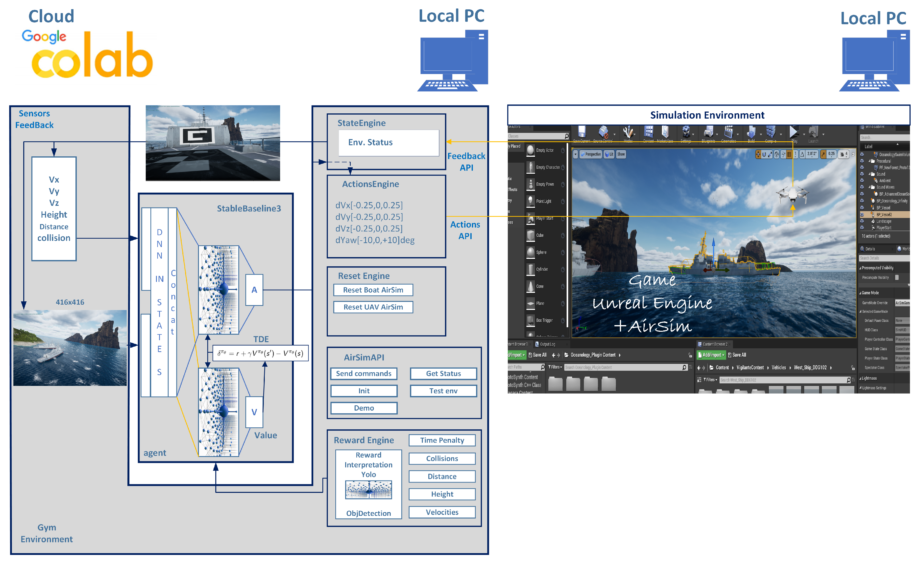
Figure 2.
RL-Based Architecture for Autonomous Drone Landing on Maritime Vessels
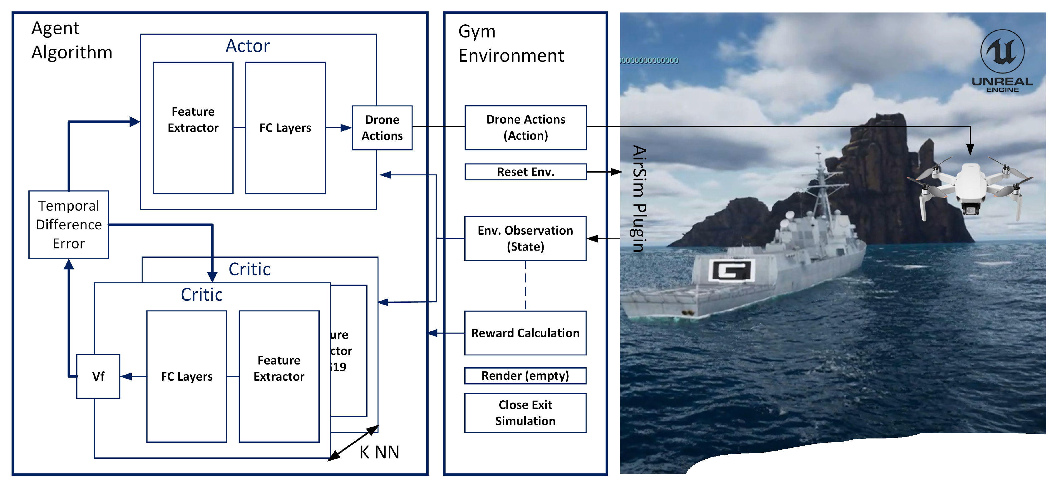
Figure 3.
Unreal Engine 4.27 Ocean Simulation Environment.
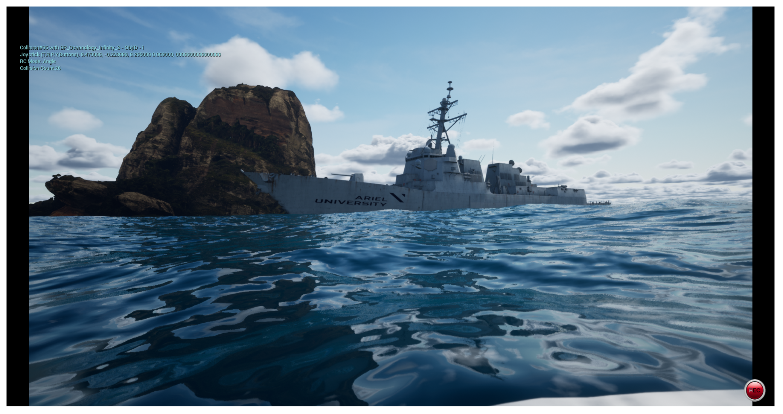
Figure 4.
Training metrics for PPO agent: (left) explained variance indicating critic accuracy, and (right) entropy loss reflecting policy stochasticity.
Figure 4.
Training metrics for PPO agent: (left) explained variance indicating critic accuracy, and (right) entropy loss reflecting policy stochasticity.
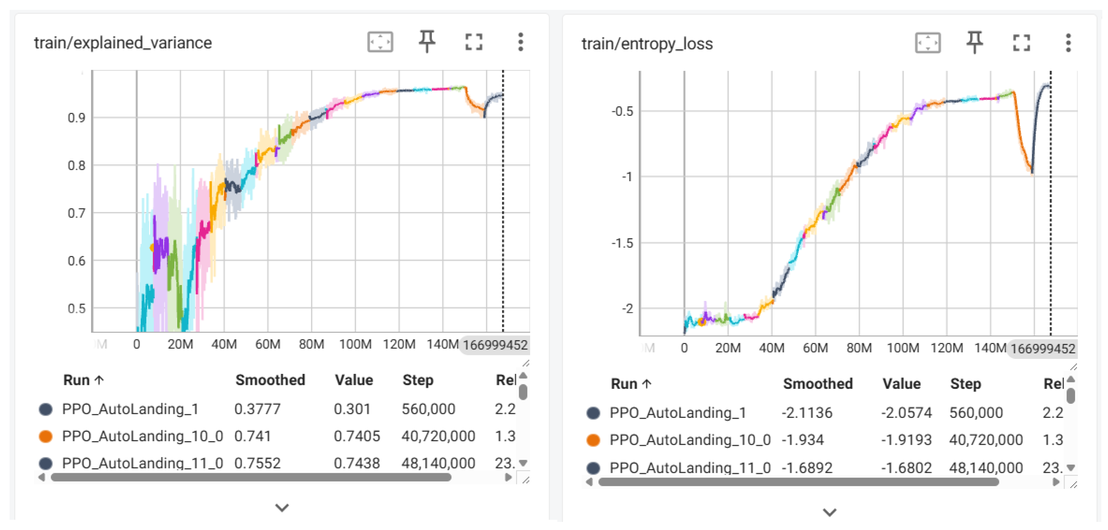
Figure 5.
Training eval metrics: (left) mean episode length and (right) mean episode reward. These metrics reflect the agent’s task completion efficiency and reward optimization during training.
Figure 5.
Training eval metrics: (left) mean episode length and (right) mean episode reward. These metrics reflect the agent’s task completion efficiency and reward optimization during training.
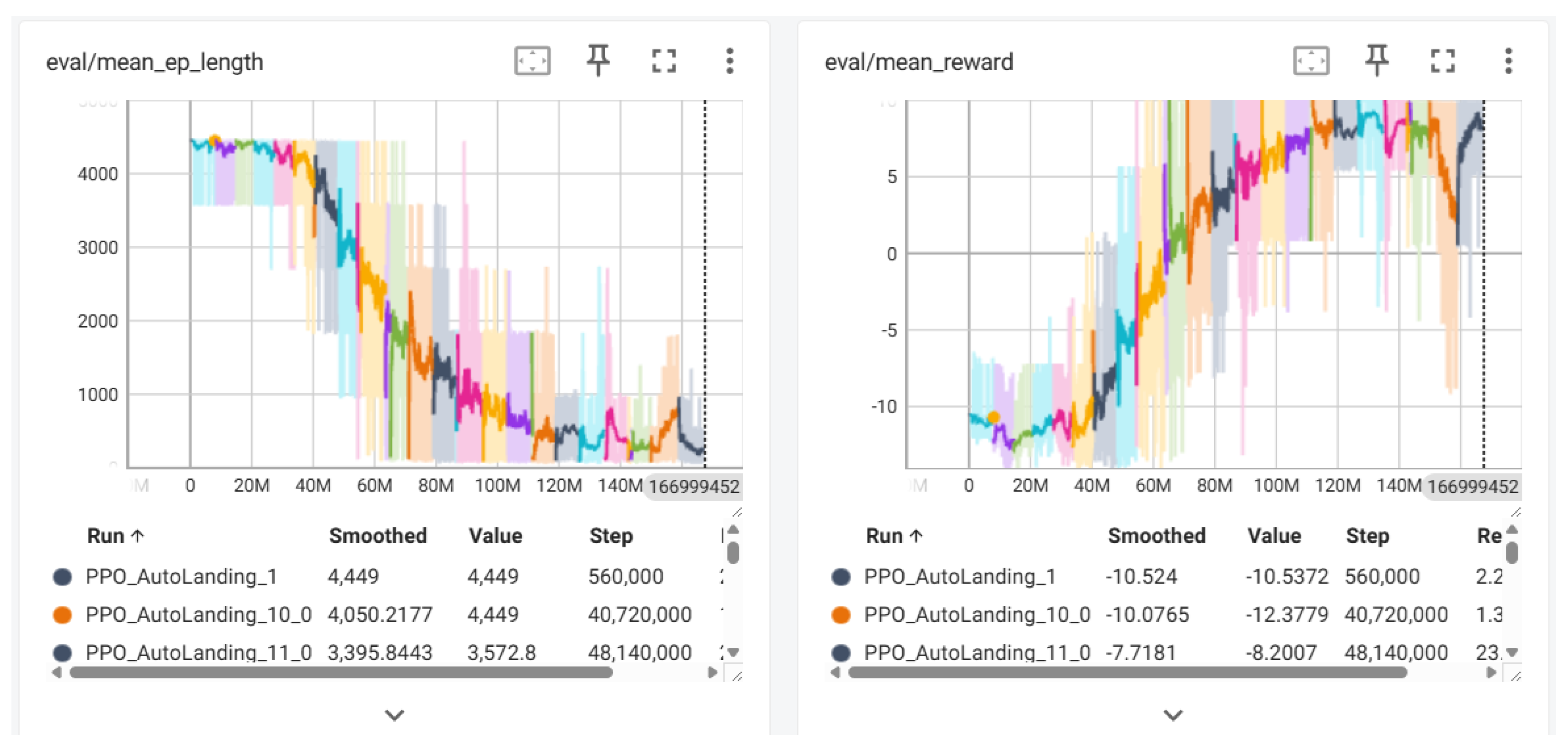
Figure 6.
Auto landing using reinforcement learning.
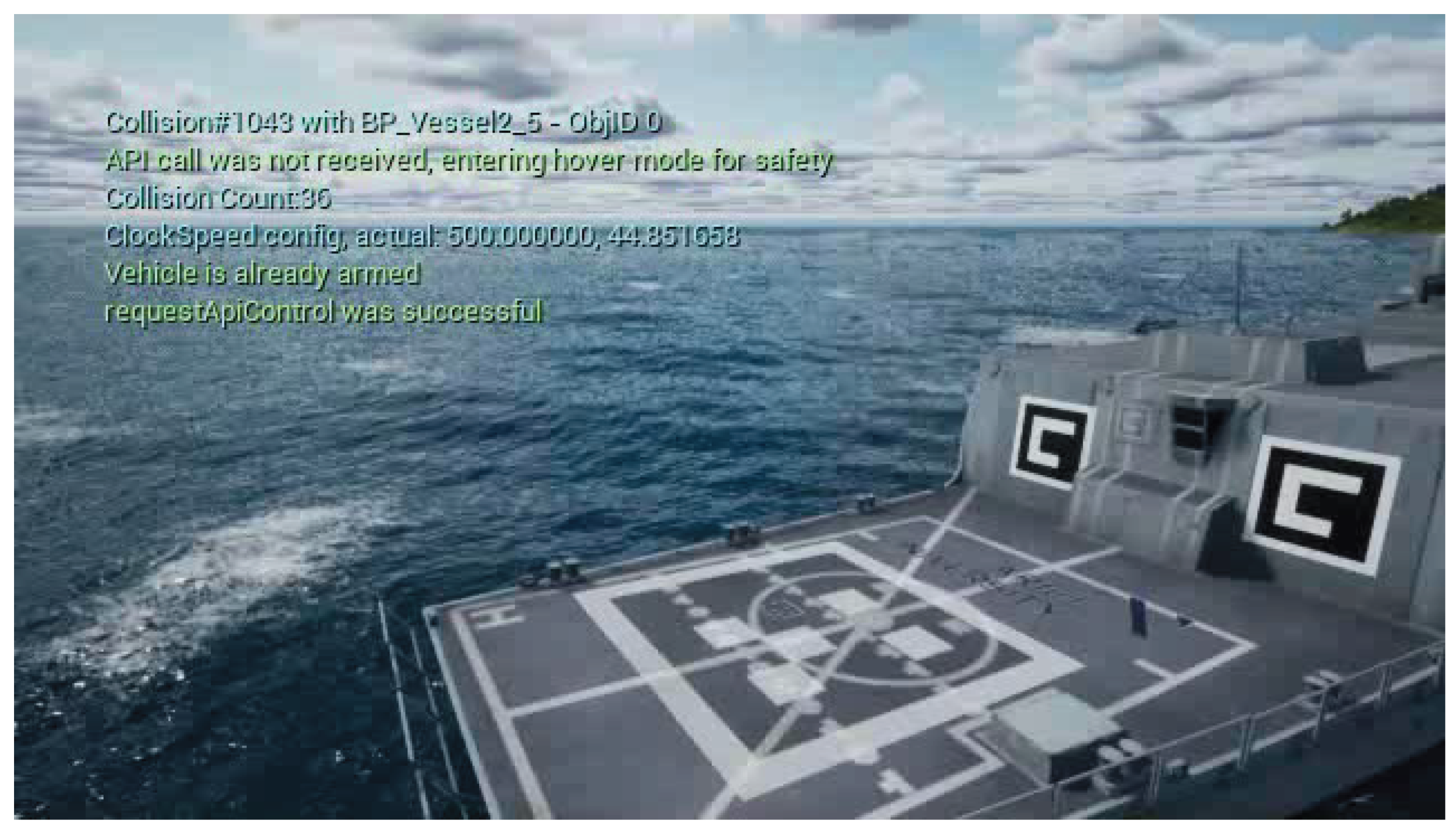

Table 1.
Discrete action mapping used in the UEAIRSIM environment.
| Action Index | Control | Description |
|---|---|---|
| 0 | Forward motion | |
| 1 | Rightward motion | |
| 2 | Ascend | |
| 3 | Backward motion | |
| 4 | Leftward motion | |
| 5 | Descend | |
| 6 | Yaw rotation (clockwise) | |
| 7 | Yaw rotation (counter-clockwise) | |
| 8 | No Operation | Hover |
Disclaimer/Publisher’s Note: The statements, opinions and data contained in all publications are solely those of the individual author(s) and contributor(s) and not of MDPI and/or the editor(s). MDPI and/or the editor(s) disclaim responsibility for any injury to people or property resulting from any ideas, methods, instructions or products referred to in the content. |
© 2025 by the authors. Licensee MDPI, Basel, Switzerland. This article is an open access article distributed under the terms and conditions of the Creative Commons Attribution (CC BY) license (http://creativecommons.org/licenses/by/4.0/).
Copyright: This open access article is published under a Creative Commons CC BY 4.0 license, which permit the free download, distribution, and reuse, provided that the author and preprint are cited in any reuse.


